the Creative Commons Attribution 4.0 License.
the Creative Commons Attribution 4.0 License.
 | 10 Apr 2018
Multi-year analysis of distributed glacier mass balance modelling and equilibrium line altitude on King George Island, Antarctic Peninsula
Damián A. López
Adrián Silva-Busso
The South Shetland Islands are located at the northern tip of the Antarctic Peninsula (AP). This region was subject to strong warming trends in the atmospheric surface layer. Surface air temperature increased about 3 K in 50 years, concurrent with retreating glacier fronts, an increase in melt areas, ice surface lowering and rapid break-up and disintegration of ice shelves. The positive trend in surface air temperature has currently come to a halt. Observed surface air temperature lapse rates show a high variability during winter months (standard deviations up to ) and a distinct spatial heterogeneity reflecting the impact of synoptic weather patterns. The increased mesocyclonic activity during the wintertime over the past decades in the study area results in intensified advection of warm, moist air with high temperatures and rain and leads to melt conditions on the ice cap, fixating surface air temperatures to the melting point. Its impact on winter accumulation results in the observed negative mass balance estimates. Six years of continuous glaciological measurements on mass balance stake transects as well as 5 years of climatological data time series are presented and a spatially distributed glacier energy balance melt model adapted and run based on these multi-year data sets. The glaciological surface mass balance model is generally in good agreement with observations, except for atmospheric conditions promoting snow drift by high wind speeds, turbulence-driven snow deposition and snow layer erosion by rain. No drift in the difference between simulated mass balance and mass balance measurements can be seen over the course of the 5-year model run period. The winter accumulation does not suffice to compensate for the high variability in summer ablation. The results are analysed to assess changes in meltwater input to the coastal waters, specific glacier mass balance and the equilibrium line altitude (ELA). The Fourcade Glacier catchment drains into Potter cove, has an area of 23.6 km2 and is glacierized to 93.8 %. Annual discharge from Fourcade Glacier into Potter Cove is estimated to with the standard deviation of 8 % annotating the high interannual variability. The average ELA calculated from our own glaciological observations on Fourcade Glacier over the time period 2010 to 2015 amounts to 260±20 m. Published studies suggest rather stable conditions of slightly negative glacier mass balance until the mid-1980s with an ELA of approx. 150 m. The calculated accumulation area ratio suggests dramatic changes in the future extent of the inland ice cap for the South Shetland Islands.


Antarctic peripheral glaciers and ice caps cover an area of 132 867±6643 km2 and therefore represent about 18 % of all of earth's mountain glaciers and ice caps (Pfeffer et al., 2014). Changes in polar ice mass balance are observed as a direct consequence of changing atmospheric and oceanic conditions acting at different spatial and temporal scales, but also changes in internal dynamics (Davis et al., 2005; Payne et al., 2004; Van den Broeke et al., 2006). The Antarctic Peninsula (AP) has been warming with a rate exceeding 0.5 K decade−1 at least during the last five decades (Barrand et al., 2013; Falk and Sala, 2015a; Skvarca et al., 1999; Steig et al., 2009; Vaughan et al., 2003). This is likely caused by atmospheric and oceanic changes associated with the stratospheric ozone depletion (Fogt and Zbacnik, 2014), strengthening of the westerlies (Orr et al., 2008; Thompson and Solomon, 2002) and the increased presence of modified warm circumpolar deep water on the continental shelf (Joughin et al., 2014). This leads to changes in sea-ice season length, extent and concentration in the neighbouring seas (Abram et al., 2010; Parkinson, 2002; Stammerjohn et al., 2012). More specifically, the increase in near-surface air temperature shows significantly higher warming trends during winter months for the South Shetlands (Falk and Sala, 2015a). The east coast of the AP is mostly influenced by cold and dry air masses stemming from the adjacent Weddell Sea. In contrast, the west coast and the South Shetland Islands are directly exposed to the humid and relatively warm air masses from the South Pacific Ocean carried by the strong and persistent westerly winds. The interaction of the westerlies with the topography of the AP can lead to extreme foehn events on the eastern side (Cape et al., 2015).
Trends in surface air temperature in the AP have been analysed and discussed in several studies obtained from meteorological observations of either manned or automatic weather stations (AWSs) (Barrand et al., 2013; Chapman and Walsh, 2007; Doran et al., 2002; Falk and Sala, 2015a; Turner, 2004; Turner et al., 2005), sometimes complemented by satellite remote sensing data (Fahnestock et al., 2002; Shuman and Stearns, 2001; Steig et al., 2009). These studies congruently show the statistical significance of the observed positive trends in near-surface air temperatures of approx. 2.5 K over the last five decades along the AP and the strong climatic change in the AP on a regional scale. Different drivers of the observed changes have been identified for winter and summer seasons: winter sea ice concentration and mean sea level pressure anomalies are strongly connected with tropical variability, i.e. the El Niño–Southern Oscillation (Bromwich et al., 2000; Meredith et al., 2004; Yuan, 2004), whereas changes of summer month's atmospheric circulation are driven by stratospheric ozone depletion and greenhouse gas concentrations (Perlwitz et al., 2008; Thompson and Solomon, 2002; Thompson et al., 2011; Turner et al., 2009). The seasonal variability is represented by the Southern Annular Mode (SAM) index. The SAM is a low-frequency mode of atmospheric variability that describes the north–south movement of the westerly wind belt around Antarctica. It shows high a positive numbers during fall–winter, associated with a contraction of the Antarctic high-pressure cell, and a variability that is of the same order of magnitude as the linear trend observed over the past four decades (Falk and Sala, 2015a).
As a consequence of the observed warming, striking glaciological changes have happened along the whole length of AP's western and eastern coasts. Studies along the AP show basal and surficial enhanced melting on ice shelves accompanied by subsequent collapse (Braun et al., 2009; Skvarca et al., 2004), widespread glacier acceleration and thinning (De Angelis and Skvarca, 2003), grounding line and calving front retreat (Rau et al., 2004; Rignot et al., 2011) and others. Ice shelves and glaciers of the AP region have been under a generalized retreat and disintegration trend at least during the last five decades (Braun et al., 2009; Rott et al., 1996; Scambos et al., 2008, 2000; Shepherd et al., 2003; Skvarca et al., 1998, 2004). Ongoing atmospheric and cryospheric change are directly linked to profound changes of the adjacent ocean (Meredith and King, 2005). Marine species in the AP region show extreme sensitivities to environmental conditions and their changes (Abele et al., 2017; Clarke et al., 2007; Ducklow et al., 2007; Montes-Hugo et al., 2009; Peck et al., 2004; Quartino et al., 2013; Schloss et al., 2012; Smith et al., 1999). Glacial meltwater input to the coastal systems significantly changes physical and chemical properties, e.g. salinity, turbidity, light transmission and trace metals (Henkel et al., 2013; Sherrell et al., 2015). These studies rely on an accurate estimation of glacier melt.
Systematic glaciological field studies are very scarce on both sides of the AP and in especially there are none that try to sufficiently capture inter- and intra-annual variability. In this paper, we present a 6-year record of continuous glaciological observations obtained on very high temporal resolution to resolve winter melt periods and properly define the start of glacial accumulation and ablation periods. The time series is analysed with regard to climatic drivers and glacial melt is estimated to provide the necessary boundary conditions for interdisciplinary studies on the ongoing changes in the biota and species composition of the coastal waters in the South Shetland region. The following sections will describe the meteorological and glaciological data time series, evaluate calibration and validation of the glaciological model, and discuss surface mass balance and simulated glacial discharge with regard to seasonal and interannual variability. Finally, results of equilibrium line altitude (ELA) and accumulation area ratio (AAR) are used to assess future glacier extent.
The main scientific objective of this paper is to investigate the impact of the concurrent climatic conditions on meltwater discharge to the coastal environments and the glacier ELA, which sets the boundary conditions for the observed environmental change.
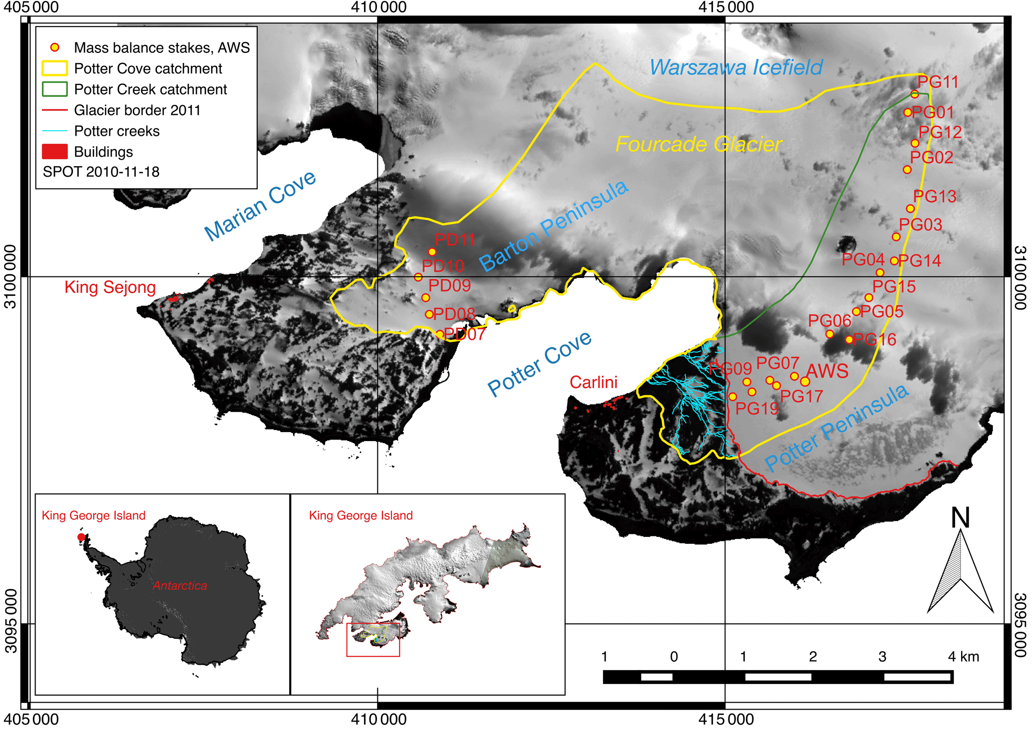
Figure 1Map of research area on King George Island (South Shetland Islands, northern Antarctic Peninsula) including the locations of our own installations and external data time series. Potter creek basins of Potter North and Potter South with drainage channels and mass balance stake locations along two transects, PG0x and PG1x (where x is a placeholder for stake number), in the catchment area. Background: SPOT-4, 18 November 2010, © ESA TPM, 2010.
King George Island (KGI) is the largest of the South Shetland Islands, located 130 km from the northwestern tip of the AP (see Fig. 1). The coast and the slopes facing north are relatively uniform and smooth, whereas the south-facing coast and slopes are rugged and steep. Around 90 % of its 1250 km2 area is covered by a polythermal ice cap and is influenced by its maritime climate. Rückamp and Blindow (2012) have surveyed a significant part of it, finding that the mean ice thickness is approx. 240 m, with a maximum value of 422 m. The maximum elevation is 720 in the central ice dome, with frequent secondary maxima of about 500–600 across the island (Rückamp et al., 2011). The ice cap is divided into drainage basins according to the underlying geological structure (Braun and Hock, 2004). The different draining glaciers end either on land or as tidewater glaciers. Most of the glacier systems on the South Shetland Islands have shown significant retreats in recent past (Birkenmajer, 2002; Braun and Gossmann, 2002; Cook et al., 2005; Rückamp et al., 2011). The Warszawa Icefield covers the southwestern part of KGI including the Potter Peninsula. It includes two tidewater glaciers: Polar Club Glacier and Fourcade Glacier. The latter drains into Potter Cove. Our data were mainly obtained on these two glaciers or in the neighbouring areas (see map in Fig. 1). Jiahong et al. (1998) and Ferron et al. (2004) report an annual average surface air temperature of −2.4 and , respectively. Falk and Sala (2015a) show a strong positive trend in surface air temperature especially in the winter, whereas for the summer month December the trend is slightly negative over the past four decades. In general, days with temperatures above freezing are rarely absent in winter and are frequent in summer. The occurrence of temperatures above the melting point all year round is well recorded by thick and multiple ice lenses even in high elevations of the ice cap. Air temperatures above the melting point are generally associated with presence of low-pressure systems and advection of warm and moist air from the mid-latitudes over the surrounding oceans often resulting in precipitation in form of rain (Parish and Bromwich, 2007).
In this study, a physical-process-based, fully distributed energy balance model is applied to estimate glacier melt and glacier runoff into the Potter cove. The temporal resolution is defined by the resolution of the meteorological input data, which were sampled to hourly values. The spatial resolution is defined by the spatial input grids of the digital terrain model (DTM), the surface facies, aspect and slope, etc. First, the meteorological data sets, quality control and gap filling are discussed. Second, the glaciological measurements and post-processing are reviewed. Third, the glaciological model is described, and the necessary input grids are defined.
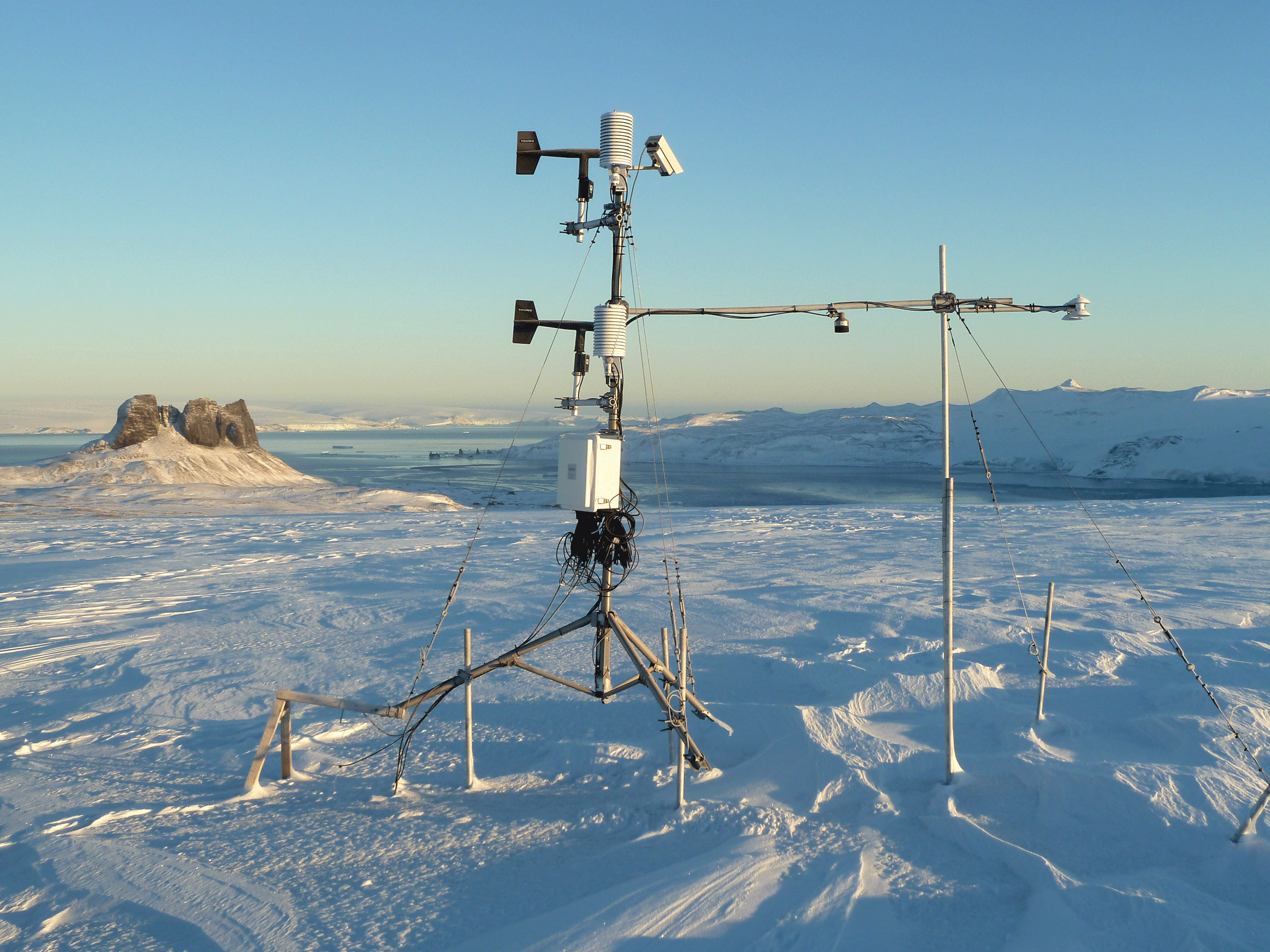
Figure 2AWS installed on the Fourcade Glacier with view to the Potter Cove and Three Brothers Hill. The photo was taken during winter on 30 May 2012.
3.1 Meteorological data sets
3.1.1 Meteorological measurements on Fourcade and Polar Club glaciers, Potter Peninsula, KGI
An AWS was installed in November 2010 at 62∘14′09.8 S and 58∘36′48.7 W at 196 , close to the approximate divide of Fourcade and Polar Club glaciers, which are both part of Warszawa Icefield. The AWS is equipped with wind anemometers and vanes (Alpine Wind Monitor); air temperature and relative humidity sensors (HMP155A) at 1.4 and 2.5 m above ground; and snow and ice temperature measurements (107 thermistor probes) installed at 10, 5 and 1 m depth in the glacier and 0.1 and 0.3 m above ground to measure snow temperature during winter. The AWS included a four-component radiation sensor (NR01) for up- and downwelling long- and shortwave radiation fluxes, two narrow-field infrared temperature sensors (IR120) facing northwest and southeast at a zenith angle of 40∘ to measure surface temperatures, and a sonic ranging sensor (SR50A) installed at an initial height of 1.9 m to measure surface elevation changes. For data acquisition and storage, a CR3000 Micrologger with extended temperature testing was used. The meteorological sensors were installed on a 3 m tripod that was fixed to 3 m aluminum poles drilled into the ice. The AWS is shown in Figs. 2 and 3. To ensure good quality of radiation measurements, all radiation sensors were mounted at a 3 m boom extended from the tripod and fixed to additional poles drilled into the ice. Levelling and adjustment of sensors were carried out according to ablation and accumulation. In case it was necessary outside of periods of summer field campaigns, this work was carried out by the overwintering scientist at Carlini Station. In particular at the end of the ablation season, the whole system needed to be lowered with a maximum of 2 to 3 m each year due to ablation at the AWS station. Power supply was realized with solar panels and a battery stack. Measurement rate was set to every 5 s with an averaging interval of 10 min. During the summer field campaign January–March 2012, an additional AWS (denoted as ZAWS) was installed in the accumulation area of the Warszawa Icefield at 62∘12′5.7 S and 58∘34′58.4 W at 424 to measure wind speed and direction, air temperature and relative humidity, as well as downward shortwave radiation (Li190SB) for the time period of 2 weeks. All sensors and station equipment were purchased from Campbell Scientific, Logan, Utah. Four additional air temperature and data logger sensors (UTL, Geotest Schweiz) were distributed on the investigated glaciers (62∘14′32 S, 58∘35′54 W, 144 ; 62∘13′51 S, 58∘38′05 W, 65 ; 62∘13′ 58 S, 58∘38′28 W, 36 ) to assess the spatial variability and lapse rates of surface air temperature. One UTL sensor was kept at 2 m height at the AWS site to ensure the continuity of air temperature records during power failure of the AWS. The meteorological data time series and climatology of the Potter Peninsula are discussed in detail by Falk and Sala (2015a).
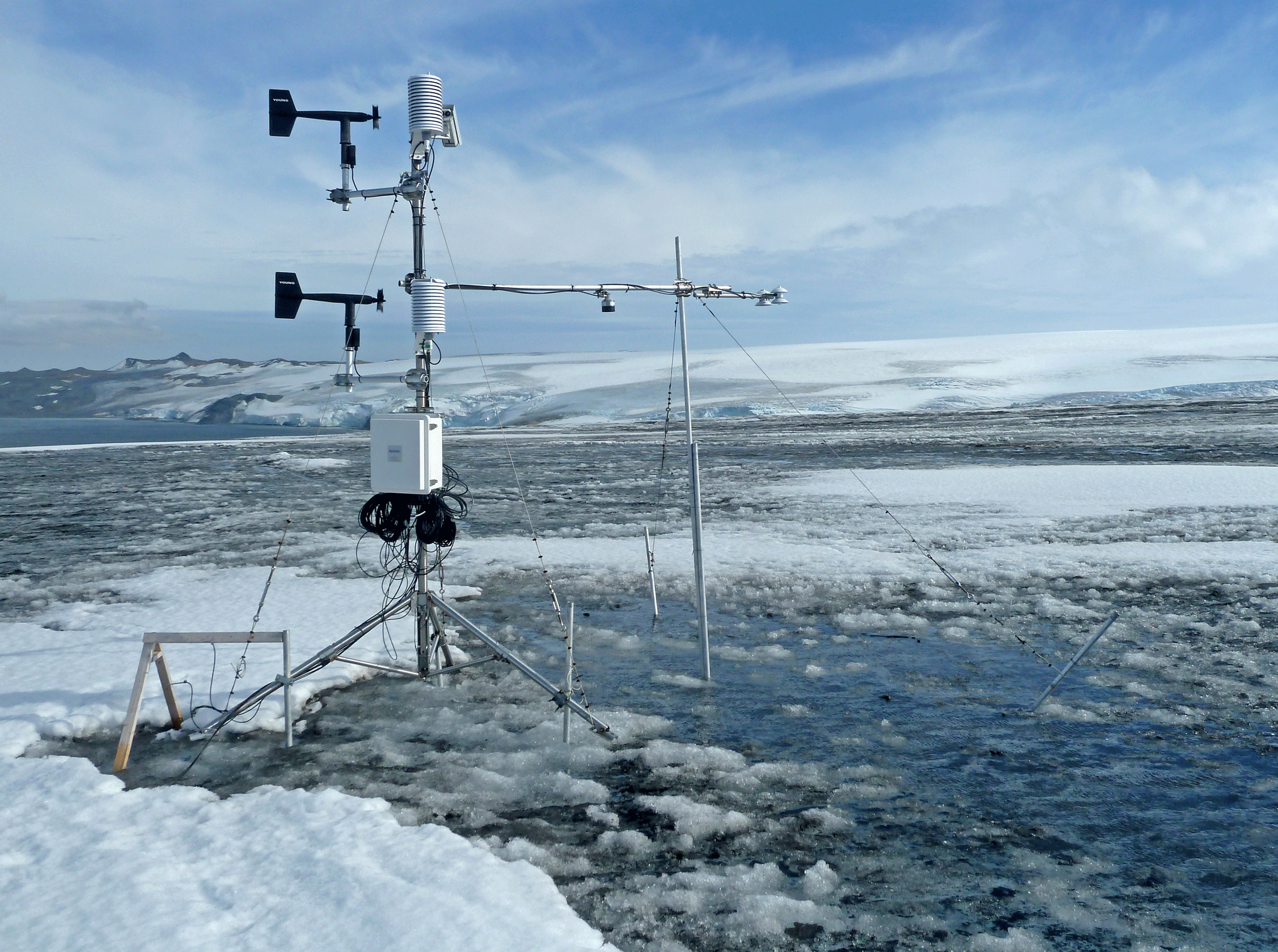
Figure 3AWS installed on the Fourcade Glacier with view to the Potter Cove and Three Brothers Hill. The photo was taken on 4 March 2012 and shows the AWS during the ablation period when pyroclastic material resurface due to melting of the winter snow layer.
3.1.2 Meteorological observations at Carlini Station
The Argentinean Carlini Station (formerly Jubany Station) is located at 62∘14′ S, 58∘40′ W at 15 at a distance of 2.7 km to the AWS. Meteorological observations are carried out by the National Meteorological Service of Argentina (SMN). The data used here represent the time period from 1 January 2001 until 1 January 2016 and contain 3-hourly observations of surface air temperature, wind direction and velocity, barometric pressure and cloudiness (SMN, 2016). This time series was resampled to hourly data by linear interpolation and smoothed by applying a moving average with a 24 h window to yield a more realistic daily course. The data set was used to investigate lapse rates between the AWS and Carlini Station in order to gap fill the time series at the AWS during power outages. Details will be discussed in the following sections on meteorological post-processing and gap filling.
3.1.3 Long-term climate data set of meteorological observations at Bellingshausen Station
The Russian Bellingshausen Station is located on Fildes Peninsula of KGI at S, W at about 14 at a distance of 18.5 km to the AWS. The Bellingshausen climate observations are on 6-hourly measurements of barometric pressure, surface air temperature, dew point temperature, relative humidity, total cloud and low cloud cover, surface wind direction, surface wind speed and precipitation. This time series starts in October 1968 and it is available in 6-hourly resolution (Martianov and Rakusa-Suszczewski, 1989). The time period for the analysis of this paper is from November 2010 to December 2015. The data used here were taken from AARI (2016) and were downloaded from the Russian weather data centre (http://wdc.aari.ru/datasets/). This data set was used to reconstruct the precipitation time series at the AWS because the ultrasonic sensor to measure distance to the surface was malfunctioning after less than a year.
3.1.4 Meteorological data processing and gap filling
The 5-year meteorological data time series for the AWS location on the glacier of the Potter Peninsula was screened for flawed and unrealistic values caused either by instrument malfunctioning or by environmental impacts such as hoar frost. During wintertime, power outages are more likely to occur and maintenance is often prevented by unfavourable weather conditions. Gap-filling routines were implemented and are discussed in the following.
Methods using the monthly mean diurnal cycle to fill data gaps were rejected, because (a) data gaps in wintertime are by far more frequent and also the time period of missing data longer, and (b) the diurnal variability is dominated by the seasonal course. For each sensor, the data were checked for malfunctioning or other environmental impact, but also for statistical properties according to Falk and Sala (2015a). The meteorological data set was aggregated to hourly time steps to reduce computation time during the modelling work (see Sect. 3.3).
The AWS air temperature measurements were screened for spikes (every value outside the 6-fold standard deviation of the long-term average) and air temperature readings below were discarded. The resulting gaps (11.6 % of the data set) were filled with records of the UTL air temperature and, where not available, were extrapolated from Carlini (CAR) Station air temperature observations based on the monthly mean adiabatic lapse rate analysis carried out by Falk and Sala (2015a).
Apart from a crossing of a synoptic frontal system, sudden spikes to low values in the barometric pressure are usually associated with problems and sudden drops in the power supply. All values below 930 hPa were thus disregarded. The 5-year average of the barometric pressure sensor computes to 967 hPa with a maximum value of 1009 hPa. Data gaps (25 % of the data set) were then filled by extrapolating the meteorological observations at Carlini Station applying the hydrostatic equation:
where the barometric pressure pCAR is the resampled time series at Carlini Station, Δz the elevation difference, RL the specific gas constant and TAWS the AWS absolute air temperature in Kelvin.
The 2 m wind velocity was screened for sensor malfunctioning. The cleaned 5-year statistics show a linear relationship between the horizontal wind speeds measured at Carlini Station and the AWS on the glacier of
This relation was used to fill the gaps in the time series of the AWS wind speed observations (25 % of the data set).
The search of a similar relationship for the relative humidity yielded a linear regression between the time series at Carlini Station and at the AWS with a very poor correlation coefficient of R2=0.3. The comparison of first-order statistics shows that
Generally, the value range of relative humidity is between 60 and 100 %. The diurnal variability is usually of the same magnitude (σRHAWS≈0.4). For this value range the error is thus acceptable. Values for the relative humidity are generally very high at the AWS site; 25 % of the complete data set of relative humidity were gap filled.
Ice temperature measurements were taken from the lowest sensor level, originally installed at 10 m depth in November 2010. The extensive ablation over the years led to a siginficant change in sensor depth over time. The 5-year statistics reveal that ice temperatures do not drop below . The near-surface levels of ice temperature measurements include values lower than this minimum value and higher than 0 ∘C concurrent with a high diurnal variability due to direct contact of the sensor with either meltwater or air. Hence, these periods are excluded from the measurements. This affected 8 % of the data set. Figure 4 shows the course of ice temperature over 5 years in the lowest level.
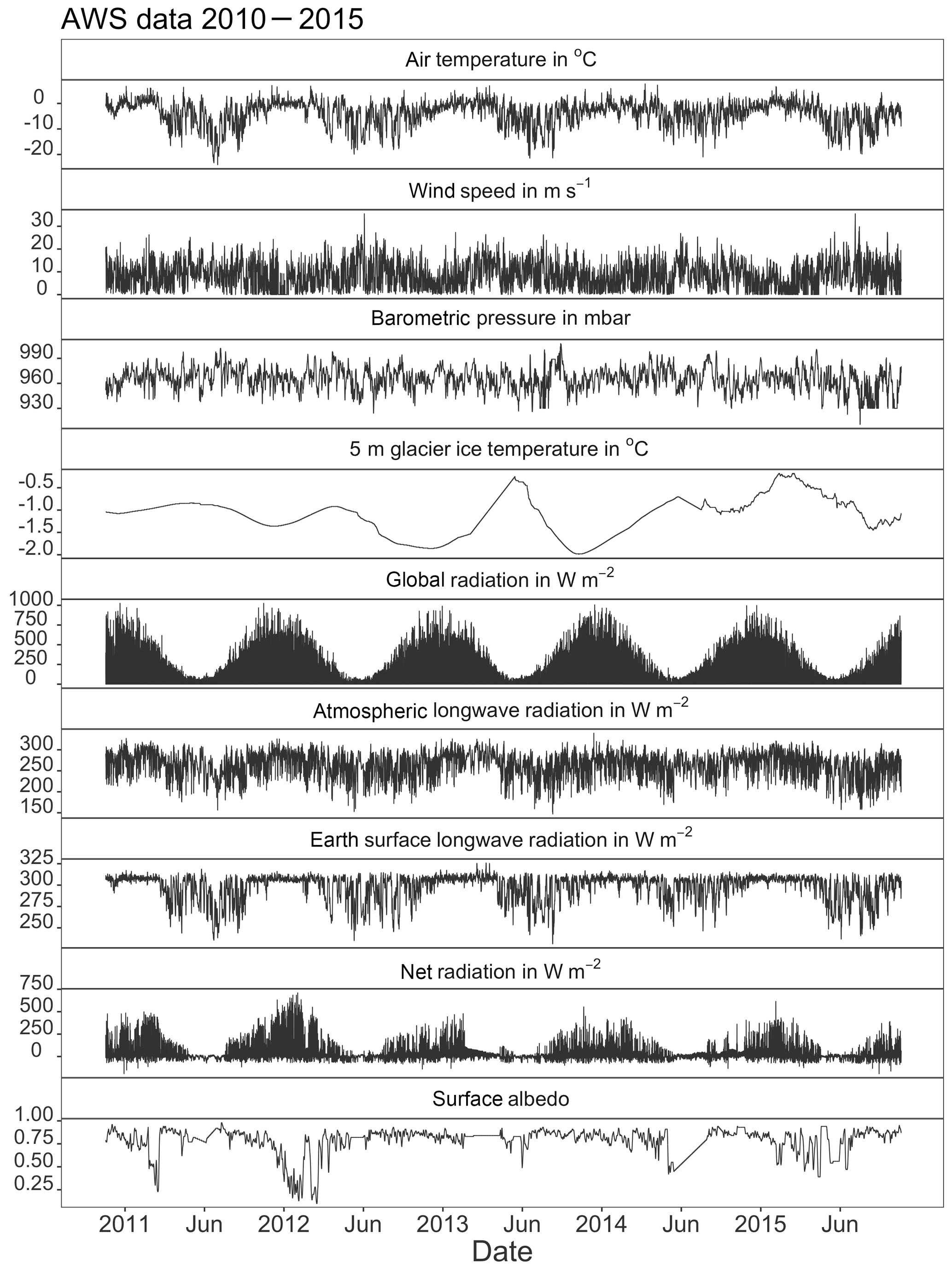
Figure 4Meteorological time series (gap-filled) aggregated to hourly resolution at the AWS site on the Fourcade Glacier, King George Island, during the time period November 2010–November 2015.
The cloud coverage data were taken from the observations (cloud coverage c8 in one-eighth of total sky area) at Carlini Station, smoothed with a 48 h window. This window size is well adjusted not to eliminate the synoptic changes between low-pressure systems, usually associated with overcast sky, and high-pressure systems over continental Antarctica that are often accompanied with clear sky. The timescale of these changes are considered to be at least 3 days to 1 or 2 weeks. The cloudiness c is given in decimal format of c8 with a value range between 0 and 1.
The four-component radiation sensor is prone to icing or riming due to advection of warm, moist air masses into the region. This affects especially the upward looking sensors for long- and shortwave radiation. As criteria for detection of sensor riming, van den Broeke et al. (2004) suggest that the downward longwave radiation flux density equals the upward flux. Here, the criterion was chosen as
where LW↓ and LW↑ are the upward and downward longwave radiation flux densities, respectively. Additionally, values of were discarded. The above criterion was met on less than 1 % of the observations. Since air and surface temperatures are often around melting conditions together with overcast skies or high cloud coverage, the applied criterion was deliberately chosen as very sharp to avoid filtering real values for longwave radiation flux densities. To fill the gaps in the radiation data time series, the different up- and downward flux densities of the long- and shortwave components were simulated by applying basic geographic and astronomic equations (Campbell and Norman, 2000) using the Julian day (J), local time (t), location information (longitude θ and latitude ϕ) in decimal-degree, absolute surface air temperature (Ta) in K, barometric pressure (Pa) in kPa, absolute surface temperature (Ts) derived from ice temperatures and upward longwave radiation measurements, cloudiness in decimal numbers (c) and the gap-filled (33 %) albedo measurements (α).
The optical air mass number is given for by , where ψ is the solar zenith angle. The atmospheric transmittance τ is calculated by adapting Gates (1980) to
The top-of-atmosphere (TOA) solar incidental radiation flux (SWTOA) is then computed by and the total solar incidental radiation flux to the surface as the sum of direct () and diffuse () components by
The solar radiation reflected (Kup, sim) at the surface is then calculated by multiplying the albedo to the simulated downward shortwave flux, i.e. the sum of diffuse and direct radiation flux.
The downward component of the longwave radiation budget at the surface is calculated using the emissivity of the atmosphere () (Monteith and Unsworth, 1990) to estimate the emissivity under cloud coverage (εac):
Applying the Boltzmann law this gives for the longwave downward component (LW↓)
and for the longwave upward component (LW↑) with a surface emissivity of ε=0.9
The statistics of the simulated radiation fluxes are then compared to the statistics of the measured time series, resulting in correlation coefficients generally above R2>0.7. The simulated longwave fluxes were adjusted to the observations by fixating the mean values of the simulated to the observed values. A difference in long-term average of 29 and 35.5 W m−2 was added to the simulated atmospheric longwave emittance and simulated earth's longwave emittance, respectively. The comparison of simulated shortwave fluxes to the long-term observations suggested a further refinement of the impact of cloud coverage on the shortwave radiation fluxes according to
with an R2=0.7. The overall comparison of the simulated (sim) and observed (obs) net radiation flux resulted in a linear regression with very good correlation:
The root-mean-squared error amounts to 39 W m−2 and the mean bias deviation to 10 W m−2. The remaining data gaps were closed using the simulated and fitted shortwave radiation fluxes. In summary, about 50 % of the shortwave and upward-facing radiation data needed to be gap filled with the simulated data, whereas only 25 % of the earth's longwave radiation data were identified as missing or flawed data.
Accumulation measurements based on sonic ranging are available during November 2010 to May 2011 and March 2012 to November 2012. Outside these periods, accumulation was reconstructed using the readings of the Bellingshausen 6-hourly precipitation data. These were resampled to hourly data time series by linear interpolation, smoothed and normalized with the total daily sum. The mass balance stake (MBS) data at the AWS location were then used as an envelop for the daily sums of the resulting accumulation time series. Figure 4 shows the resulting quality-controlled and gap-filled data time series of the meteorological variables.
3.2 Glaciological measurements on Fourcade Glacier, Potter Peninsula, KGI
Two transects of MBSs were installed from the top of the Warszawa Ice Dome down to the border of the glaciers Fourcade and Polar Club to serve for calibration and validation of modelling efforts (see Fig. 1 and Table 1). Additional transects were installed along glacier ridge on Barton Peninsula on the Fourcade Glacier on the opposite side of the Potter Inlet. The stakes were measured at the beginning and end of each summer field campaign in November 2010, February–March 2011 and January–March 2012 and every 10 to 14 days, depending on weather conditions, during the austral winter 2012 up to March 2013. During the austral winter 2013 and until May 2016 the measurements were conducted every 20 to 30 days. MBS readings during winter months were mostly conducted in the ablation area of the glacier except for four stakes (PG04, PG14, PG05 and PG15). Additional measurements in the accumulation area were carried out during summer and fall seasons. The high wind speeds, high precipitation rates during austral winter and potentially the material of the stakes (aluminum) resulted in regular loss of the stakes in the accumulation zone of the Warszawa Icefield and thereby the loss of the time series. For the measurements of stakes that were not protruding vertically from the ice but at an inclination caused by the high wind speeds, a geometric correction was applied to yield the correct exposition length. During the summer field campaigns November 2010 to March 2013, repeat measurements with differential GPS (DGPS) at static points of the MBSs yielded an average velocity for the lower transect up to elevations of approx. 250 m of below 1 m a−1 and up to 6.3 m a−1 for the MBSs on the upper glacier. Figure 5a shows a sampling at the MBS transect.
Table 1Locations of the mass balance stake (MBS) at the AWS and the transects (PG0x and PG1x) on Potter Peninsula and the mass balance stake transect (PDx) on Barton Peninsula, Fourcade Glacier, on King George Island (see map in Fig. 1), during the time period November 2010 to December 2016.
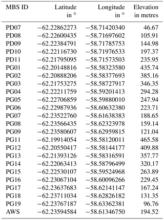
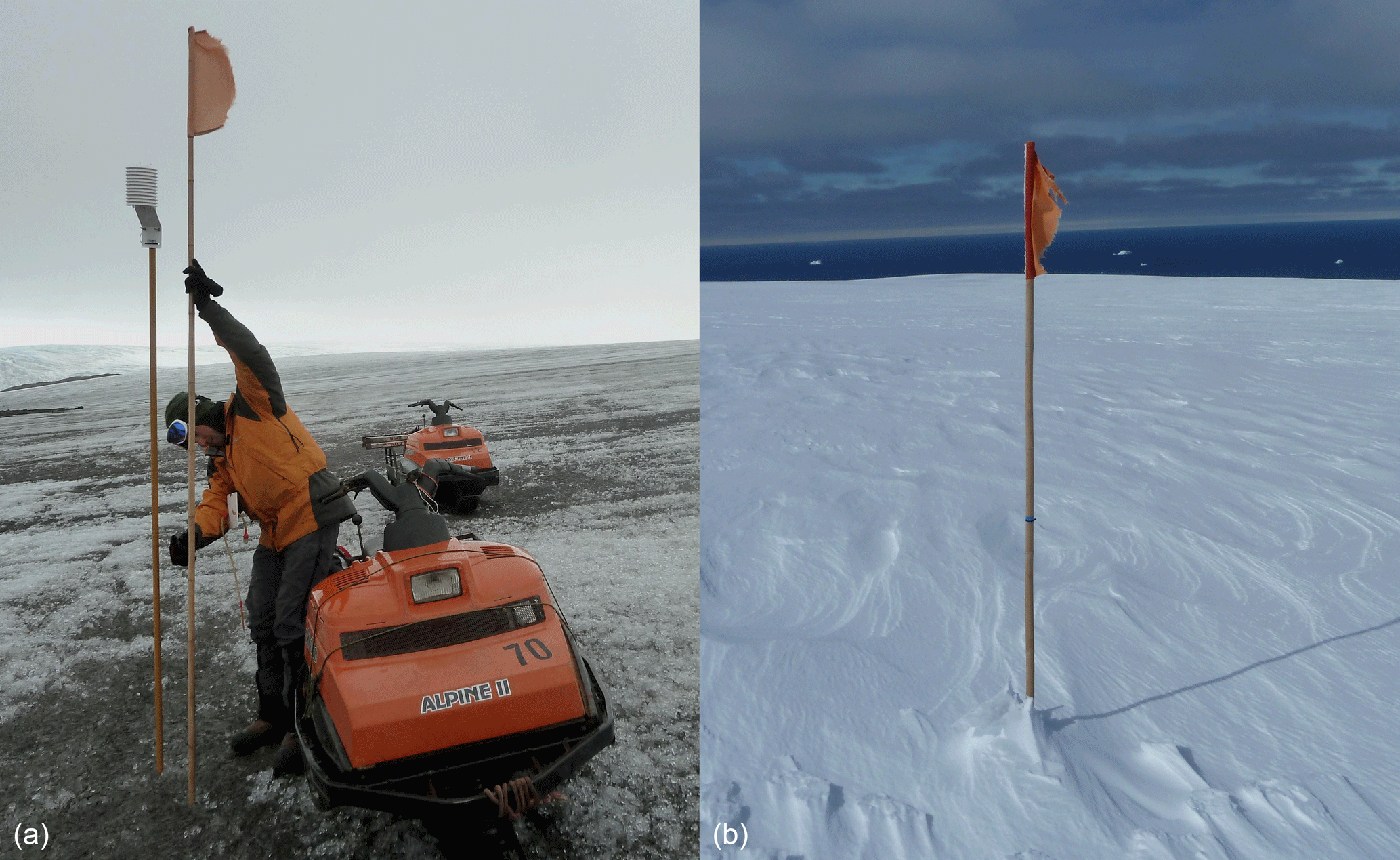
Figure 5MBS transects installed on the Fourcade Glacier during the ablation period on 28 March 2012 (a) and during the accumulation period on 10 November 2012 (b).

Figure 6Displayed is the time series of snow density observations on the Fourcade Glacier, Potter Peninsula, during the time period June 2012 to February 2016 (a). Red lines are linear regression lines from onset of winter accumulation until the end of the glaciological year. The snow density profile measurements along the mass balance stake transects (see Fig. 1) on the dates 21 January 2014 (summer) and 10 March 2014 (late fall) on the Fourcade Glacier, Potter Peninsula, are shown (b). Measurements were taken at a depth of 30 cm.
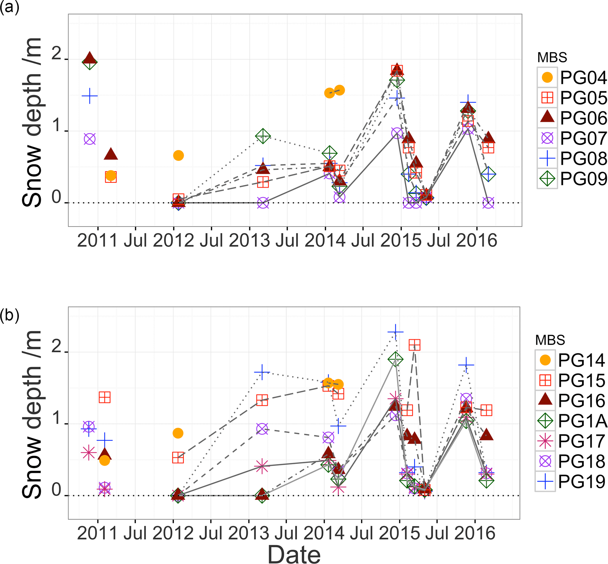
Figure 7(a) Time series of snow depth measured at the two mass balance stake transects (PG0x and PG1x) on the Fourcade Glacier, Potter Peninsula, during the time period November 2011 to May 2016. (b) Snow depth profile with elevation measured during summer and late fall 21 January and 10 March 2014. The location of the individual mass balance stakes (MBS) is shown in Fig. 1.
Snow density samples were taken with an aluminum snow density cutter (SnowHydro, Fairbanks, Alaska) with a defined volume of 0.001 m3 and a balance scale with an accuracy of 0.1 g (Carl Roth GmbH, Germany) calibrated at least once each summer campaign. For the snow density sampling, a snow pit of about 0.5 m depth was dug out and at least three sample volumes, extracted at a depth of about 0.3 m by putting the snow cutter horizontally into the pit wall, were then averaged. The snow depth was measured with a regular snow sonde used as mountaineering equipment. Around each stake about 10 measurements were taken and then averaged. Snow densities were measured 15 November 2010 in the glacier ablation zone and on 7 March 2011 in the glacier accumulation zone, yielding a snow density of ρs=503 ± 16 kg m−3 and ρs=488 ± 20 kg m−3, respectively. On 23 January 2012, a snow pit was dug out in the accumulation zone of the Warszawa ice cap at the additional AWS (Falk and Sala, 2015a). Snow density measurements were taken every 0.2 m up to a depth of 2 m and resulted in an average value of . The correlation with depth was found to be not significant.
Starting in June 2012 until February 2016, regular snow density values were taken together with the MBS transect measurements. A seasonality in the snow density time series is evident and presented in Fig. 6a. With rising temperatures during the austral summer and fall, the snow density also shows rather high values up to approx. 500 kg m−3. With the onset of the winter, the precipitation changes to low-density snow, which then compacts over the course of the winter. During austral winter, the overwintering scientist was responsible for the glaciological measurements of the whole campaign. The snow density time series of winter 2015 shows a high variability and particularly low values, well below any observation before. Although the values by themselves are reasonable for very cold and dry conditions (Patterson, 1980), the contemporary surface air temperature measurements do not show any behaviour that would satisfy the requirements for the very low snow density observation. We therefore suspect the measurement to be affected by errors, leading to an underestimation of the snow density. This seems to have been the case during winter 2015. Thus, for the time period before June 2012 and after March 2015, mass balance and related variables were computed using the monthly averages of the period in between for snow density values. Figure 6b shows measured elevation profiles of snow density for two dates, i.e. the beginning of summer and late fall. The upper profiles show less variability and no significant change for the accumulation area above 250 m, whereas for the lower transect the absolute value of snow density and the variability of the observations is considerably higher.
These findings are supported by the snow depth measurements (DS) displayed in Fig. 7, which show the transects PG0x and PG1x where x is the index of the actual stake number. The snow depth measurements were carried out as far as possible at the beginning and the end of the summer campaigns and, since 2012, on a more regular basis together with the accumulation and ablation measurements of the MBSs. In a circle around the MBS at a distance of 1 to 2 m, about 5 to 10 snow depth measurements were taken with a snow sonde, with the average value taken as snow depth. Due to frequent rain events, ice lenses in the snow layer were common. These values were excluded. The lowest MBSs of both transects show a higher snow accumulation than the stakes at higher elevation. A reasonable conclusion is a different atmospheric turbulence regime that leads to a higher snow deposition at the glacier border due to the vicinity of the glacier end moraine and moraine. Also in the snow depth measurement, the more distinct stratification of transect PG0x with elevation is evident.
The snow density and snow depth time series were used to compute the cumulative mass balance (CMB) in metres of water equivalent (m w.e.) from MBS observations along the mass balance transects shown in Figs. 8 and 9. To convert to m w.e., values needed to be divided by the density of water at standard conditions, . The mass balance stake readings were referred to the initial value measured when the stake was installed, which was later considered as the zero for each stake. The observed height change of the mass balance stake (ΔH) translated into surface mass balance change in m w.e. by
When there was a snow pack, the measured snow density ρs was used. During glacier facies conditions of bare ice, the ice density of was assumed. To convert the unit of Δb from kg m−2 to m w.e., values are divided by the density of water, .
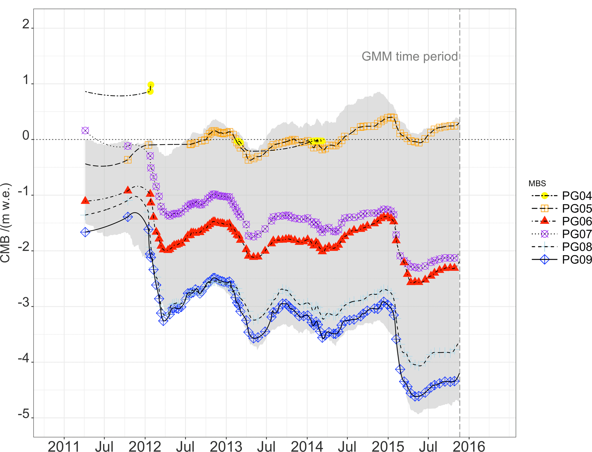
Figure 8Shown is the cumulative mass balance in m w.e. (water equivalent) measured at the calibration mass balance stake transect PG0x on the Fourcade Glacier, Potter Peninsula, during the time period November 2011 to May 2016. The location of the individual stakes is shown in Fig. 1. The lines are interpolation lines between observation points. The grey shade indicates the spread of the GMM-simulated cumulative mass balance at the stake locations PG05 to PG08.
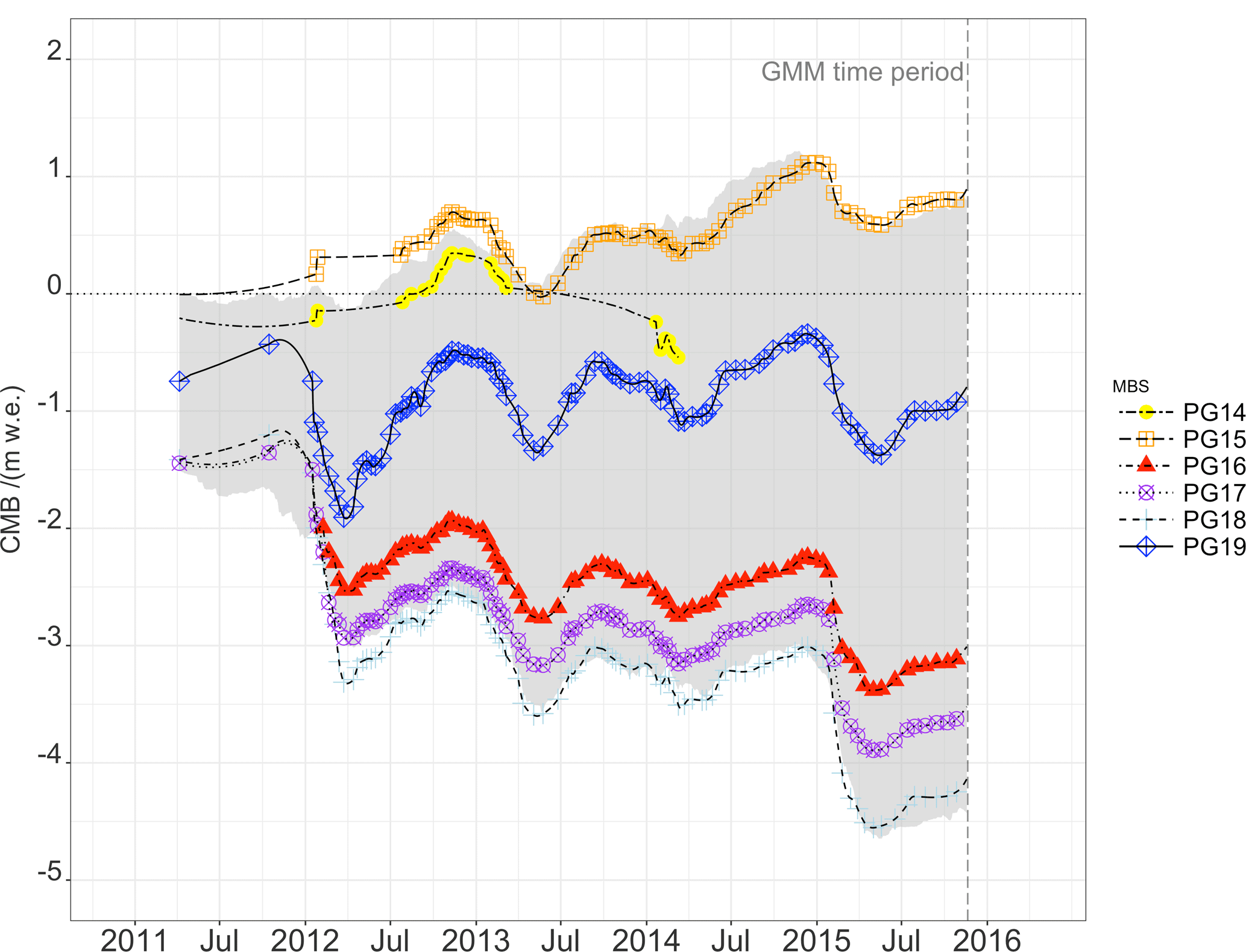
Figure 9Shown is the cumulative mass balance in m w.e. (water equivalent) measured at the validation mass balance stake transect PG1x on the Fourcade Glacier, Potter Peninsula, during the time period November 2011 to May 2016. The location of the individual stakes is shown in Fig. 1. The lines are interpolation lines between observation points. The grey shade indicates the spread of the GMM-simulated cumulative mass balance at the stake locations PG15 to PG18.
The resulting MBS time series graphs is differentiated by the transect ID PG0 and PG1. The gradual shift from ablation at the lowest MBS PG09 to accumulation at the highest MBS PG04 is clearly visible. The PG1 transect, however, does not follow this behaviour: there is considerably more accumulation at MBS PG19 than at the higher elevation PG17. Also within the accumulation zone, the expected increase of accumulation with elevation does not apply: the cumulative accumulation at MBS PG14 is considerably lower than at MBS PG15. This can be explained by the different degree of exposure to weather. KGI is prone to transient low-pressure systems connected to storm events with high wind speeds from the northwest and precipitation mostly in the form of rain, but also to katabatic winds due to influence of the Antarctic high-pressure systems with high wind speeds from the southeast (Falk and Sala, 2015a). The southern MBS transect PG1 is more exposed to these synoptic changes and prone to snow drift by the high wind speeds. MBS PG19 and partly PG18 show this extra accumulation of the snow, but PG14 also shows a lower accumulation than PG15 although elevations are reversed (see Fig. 9). For the MBS transect PG1 it can be assumed that these include effects of aeolic snow drift.
The very high temporal resolution of mass balance observation is unique for the AP region and was chosen not only to resolve the high seasonal and interannual variability of the onset of accumulation and ablation period but also to capture winter melt periods to estimate glacier meltwater runoff also during wintertime. The time series analysed here encompass 6 years, but are still ongoing. Figures 6 to 9 show the respective time series of snow density, snow depth and surface mass balance observations.
3.3 Glacier surface mass balance model
3.3.1 Model description
The glacier surface mass balance model (GMM) by Hock and Holmgren (2005) and Reijmer and Hock (2008) computes accumulation and ablation, including glacier melt and discharge, at the temporal resolution of the meteorological input data, here chosen as hourly. The GMM was run in energy balance mode and the requested climatological input consists of air temperature (θair), relative humidity (RH), wind velocity (v), shortwave downwelling radiation (Kd), precipitation (P), shortwave upwelling radiation (Ku), net radiation (Rn), longwave radiation emitted by the earth's surface (E), atmospheric longwave radiation (A), barometric surface air pressure (pair), albedo (α), ice temperature at 5 m depth (θice) and cloud cover in eighths (c8). The GMM is fully distributed, meaning that calculations of glacier surface mass and energy balance terms are performed for each grid cell of a defined model area on a digital elevation model as discussed in the last paragraph. Discharge is calculated from the water provided by melt plus liquid precipitation by three linear reservoirs corresponding to the different storage properties of firn, snow and glacier ice volumes. The energy available for melt (QM) is computed by
where G is the global (solar incidental radiation) radiation, H the sensible heat flux, λE the latent heat flux, Qground the ground or ice heat flux and QR the sensible heat supplied by rain. Global radiation, albedo and up- and downwelling longwave radiation were taken from the AWS time series. The model configuration in energy balance mode allows for the specification of average monthly air temperature lapse rates. These were taken from Falk and Sala (2015a). The roughness lengths for wind were set in the GMM configuration and used to tune the model to the mass balance stake observations at the transect PG0x. In the configuration of Braun and Hock (2004) for a summer period on the little Bellingshausen ice dome during a weeks during austral summer, a value for z0=0.0026 was chosen. This choice proved inadequate for the wider region of the Warszawa Icefield. Smeets and Van den Broeke (2008) and Heinemann and Falk (2002) found an aerodynamic roughness length of to 10−5 near the equilibrium line on the Greenland ice sheet. A study on roughness lengths and parametrizations of sensible and latent heat fluxes in the atmospheric surface layers for alpine glaciers (Brock et al., 2006) suggests a significant lower value for m, depending on the very high wind speeds and a surface that is during most summer periods characterized by slush and bare ice with water-filled gaps (see photo in Fig. 2). Here, z0=0.00005 was chosen. The roughness lengths for temperature and vapour pressure were computed according to Andreas (1987). Lapse rates for air temperature, precipitation and wind are configured in the GMM input parameters according to Falk and Sala (2015a). Air temperature, wind velocity and relative humidity were then calculated on spatial distribution over the whole area. The turbulent fluxes of latent and sensible heat were computed according to the Monin–Obukhov similarity theory considering atmospheric stability. The surface temperature is derived by the GMM by iteration from the energy balance equation, where the surface temperature is lowered in case of a negative QM until the term becomes zero. The ground or ice heat flux, otherwise neglected, is thereby considered indirectly: if the energy balance equation is negative, the surface temperature is being increased using negative surplus. No melt is allowed until the negative energy balance has been compensated for. The energy amount supplied by rain is computed by
where Tr is the temperature of rain assumed to be identical to surface air temperature.
3.3.2 Hydrological catchment definition of Potter Cove and input grids
To estimate the complete input of glacial and snow meltwater into the Potter Cove, the GMM was run in catchment configuration. The model area encompasses glacial and periglacial areas that are part of the Fourcade Glacier catchment area draining into Potter Cove. The boundary of the Fourcade Glacier is taken from Bishop et al. (2004) and refined with the analysis of glacial divides by our own kinematic differential GPS mapping of surface elevation. The surface topography is based on an analysis of TerraSAR TanDEM-X remote sensing data performed by Braun et al. (2016) with a resolution of this DTM is 10 m by 10 m. Both a resolution of 50 m by 50 m using the DTM for KGI by Rückamp et al. (2011) and a resolution of 10 m by 10 m using the DTM by Braun et al. (2016) were applied. The output of these, as well as runs using 100 and 250 m resolution for the whole of King George Island, showed no significant differences.
The GMM was applied to two different catchment areas: (1) the hydrological catchment area draining into the Potter meltwater and discharge creeks and (2) the Potter Cove catchment, i.e. the Fourcade Glacier, defined as the part of the Warszawa Icefield that drains into Potter Cove. The Potter Cove catchment has an area of 25.1 km2 and is glacierized to 94 % where the greatest non-glacierized part is located on Potter Peninsula. The map in Fig. 1 displays the catchment definitions, the location of MBS transects in the catchment area. The input data grids to the GMM are based on this DTM. The DTM published by Rückamp et al. (2011) has a spatial resolution of only 50 m by 50 m but its accuracy is rather low especially for the Warszawa Icefield due to missing in situ ground truth data. Apart from the DTM and the catchment area definition, further input grids comprising information on slope, aspect and sky view factor were calculated from the DTM. The grids containing the information of glacier facies, i.e. firn, ice and rock area, were derived from the glacier zonal mapping published by Falk et al. (2016). The grid containing initial snow water equivalent values in cm were taken from our own in situ measurements along the MBS transects and spatially extrapolated by using the elevation from the DTM. The inaccuracies of the different grids on information of glacier facies and initial snow height, are taken into account by introducing a relaxation period by duplicating the first 44 days and cutting off the first 1056 hourly data time steps of the model run. During this initialization period, the GMM adjusts the inaccurate spatial input data. After these initial 1056 hourly time steps the model's internal physics are assumed to be according to the actual state of physics of the glacier under investigation and a realistic discharge pattern established.
For the catchment boundary refinements, flow directions were calculated on the basis of the data from our own differential GPS measurements on the MBS transects taken at the glacial surface and then were interpolated to form a topography of the surface. For the austral summer 2010–2011, the drainage basins were estimated to encompass glacier elevations between 80 and 450 m with slope to the SW. The supra-interglacial drainage pattern analysis using water drainage channels on the glacier surface were identified using sensors in optical remote sensing satellite data (SPOT-4, 18 November 2010, © ESA TPM, 2010). The drainage of the mass of a glacier can be interpreted similar to a karst rock (Eraso and Domínguez, 2007). The Fourcade Glacier surface drainage shows a straight, poorly integrated and strong direction towards the southwest. The glacier divides then served for further refinement of the catchment area definition in especially of the southern part of the Potter Cove catchment (see Fig. 1).
4.1 GMM calibration and validation
The GMM run period was chosen for the 5-year period 22 November 2010 to 21 November 2015. The glaciological observations encompass the time period November 2010–May 2016, but the high-frequency data acquisition does not start before February 2012. For calibration of the GMM, the mass balance observations at the transect with transect ID (TID) PG0 were used (see Fig. 10); for validation, the MBS transect with TID PG1 (see Fig. 11) was used. In both figures, each start of the ablation period was chosen as null reference for the CMB to highlight two main drivers of the GMM deviation from observations, defined as the summer year (SY). The errors are cumulative over the course of each year starting with the ablation period (e.g. SY 2012 starts 2 December 2011; Table 2). Orheim and Govorukha (1982) found layers of pyroclastic material in ice cores from the King George Island ice cap, dating them to volcanic eruptions on Deception Island in December 1967, February 1969 and August 1970. These layers are surfacing in the ablation zone of the westward-facing side of the Fourcade Glacier on Potter Peninsula during melt periods (see Fig. 3). The dark material significantly changes the surface albedo and surface ablation. Since albedo is included in the meteorological input variables, this process is taken into account by the GMM run. The glaciological observations reflect the heterogeneous pattern of accumulation and ablation areas reported by Falk et al. (2016). Hence, spatial extrapolation of surface properties, as the albedo, is expected to add to the uncertainty of the modelling results.
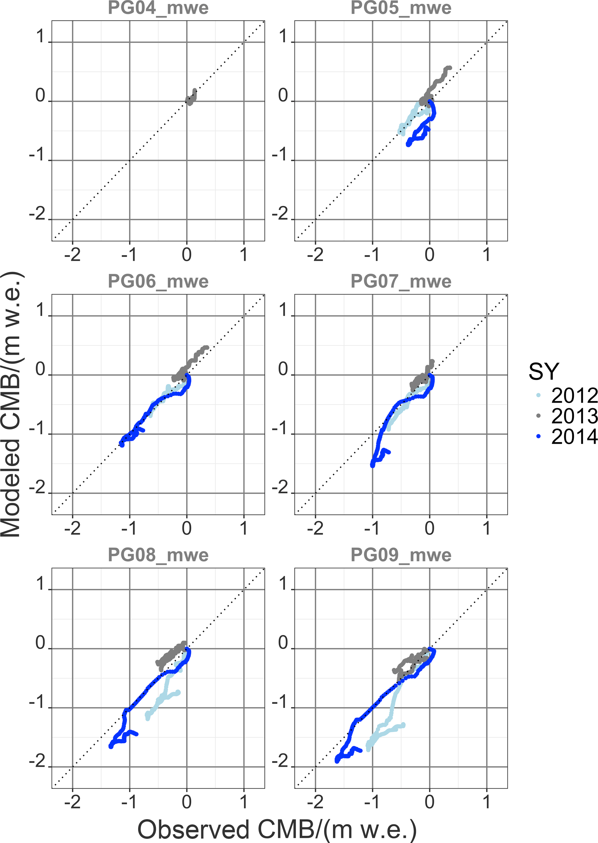
Figure 10Cumulative mass balance (CMB) from simulations with the glacier melt model (modelled CMB) and observation (observed CMB) on the Warszawa Icefield (transect ID PG0x) for calibration purposes. Year numbers give the year of start of the glaciological mass balance year. It encompasses the glaciological years 2012/13 to 2014/15.
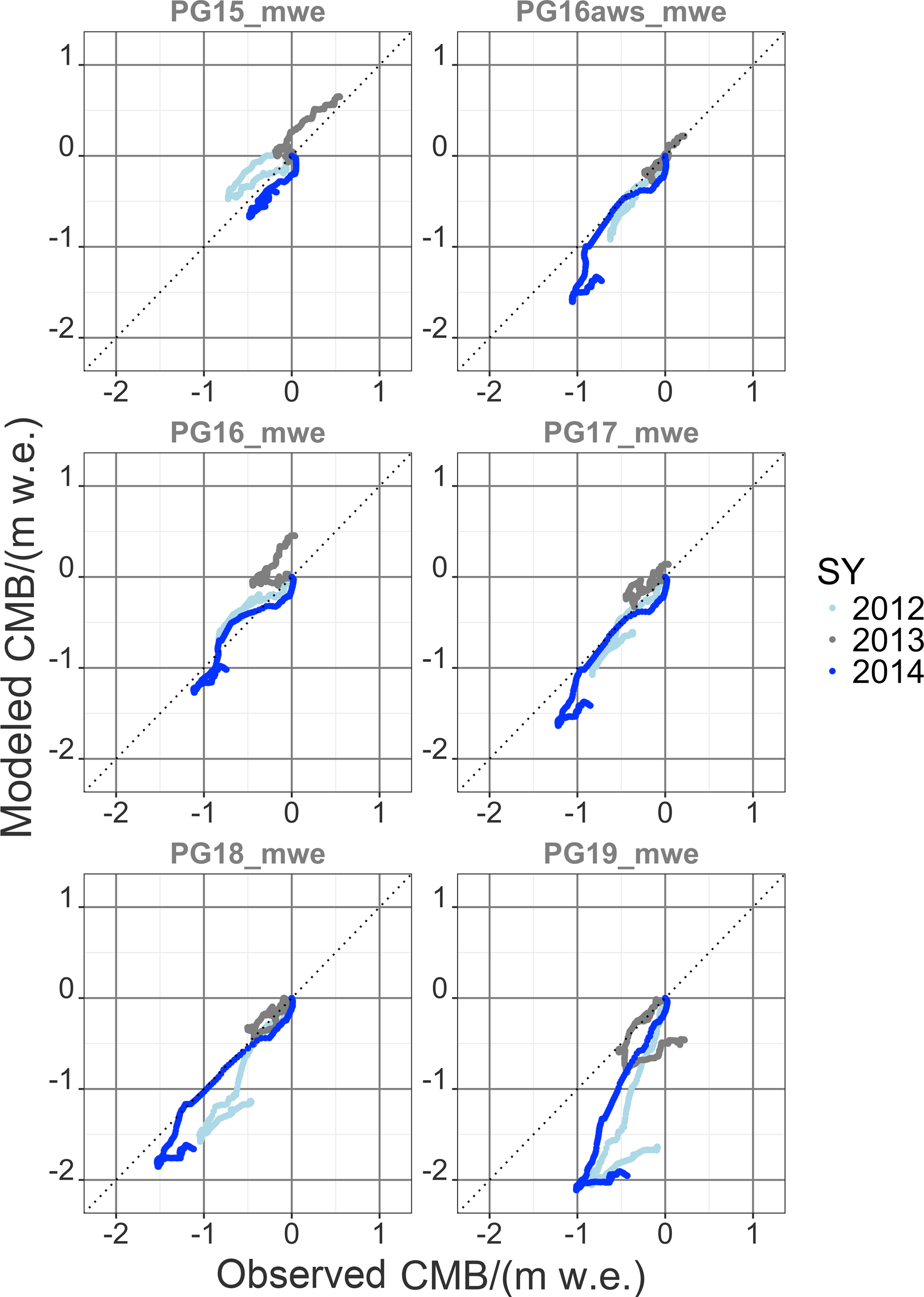
Figure 11Cumulative mass balance (CMB) from simulations with the glacier melt model (modelled CMB) and observation (observed CMB) on the Warszawa Icefield (transect ID PG1x) for validation purposes. Year numbers give the year of start of the glaciological mass balance year. It encompasses the glaciological years 2012/13 to 2014/15.
Figures 8 and 9 include the spread of the GMM output of accumulation and ablation for the DEM pixels at MBS locations PG05 and PG08 (Fig. 8) and PG15 and PG18 (Fig. 9). The GMM outputs the cumulative accumulation and ablation for 10 m by 10 m grid cells at the stake locations. Model calculations are shaded in grey. Figures 8 and 9 show that model and observations are generally in agreement. The GMM does not fully account for the spread in the observations, which is attributed to the significant snow drift due to high wind speeds and snow deposit due to turbulence at the glacier end moraine and to the high contribution of snow erosion by rain.
Figures 10 and 11 show the high interannual variability. The high frequency of observations allows one to differentiate between periods with different climatic settings. The high deviation of CMB, especially towards the end of the ablation period, shows that the GMM clearly underestimates the accumulation due to snow drift and turbulence-driven snow deposition at the glacier border (see Figs. 10 and 11). The closer the MBSs are to the glacier border, the more the effect of turbulence-driven snow deposition comes into effect.
SY 2014 contained the coldest summer in the GMM run period, with the highest amount of precipitation as well. In the beginning of the ablation period, air temperatures were below freezing and snow fall occurred together with high wind speeds. This leads to an underestimation in the simulated CMB since the GMM does not account for snow drift. Then there is a period when model and observations are in very good agreement. During the fall of SY 2014, there were frequent rain events. Since the GMM was run in catchment configuration, meaning that the model area contained also the periglacial parts of the hydrological catchment, the snow module (Reijmer and Hock, 2008) could not be applied. Refreezing processes could, thus, not be considered, and the simulated CMB is also underestimated. The accumulation period at the end of SY 2014 is again marked with the underestimation in CMB due to the disregard of snow drift in the GMM.
Apart from these two climatic boundary conditions, the model results and the glaciological observations are in good agreement, and a drift or disagreement over the 5-year GMM run period cannot be seen in the data.
4.2 Glacier surface mass balance
Cogley et al. (2011) give the annual (surface) mass balance (bn) at the end of a balance year as the sum of winter mass balance (bw), i.e. the sum of winter accumulation (cw) and ablation (aw), and summer mass balance (bs), i.e. the sum of summer accumulation (cs) and ablation (as):
All mass balances calculated here refer to the points of the MBS transects and are referred to by lowercase letters (b). Ice density is assumed to be equivalent to 0.9 kg L−1. All units are in kg m−2. Assuming an uncertainty in snow height measurements of ΔH=0.2 m to account for natural surface heterogeneity around each stake and of for the variability in snow density measurements leads to an uncertainty of Δb=0.35 m w.e. in specific glacier mass balance estimates.
Table 2Definition of beginning and end of the glaciological summer deducted from observations of local minima and maxima of the accumulation/ablation time series at the mass balance transects (PG0x and PG1x) on Potter Peninsula, King George Island, during the time period November 2010 to December 2016.
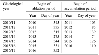
The GMM outputs for the first glaciological year 2010 (meaning 2010/11) were not considered in the further analysis due to the model spin-up for the first few months. Results for the stake locations close to the glacier border, i.e. PG09 and PG19, were excluded in the graphs, as already discussed (Sect. 3.2). The beginning and end of the accumulation and ablation period of each year are listed in Table 2 and show the seasonal shift towards late start of the ablation period until November or December and the late end of the ablation period until end of May, except for the glaciological year 2013/14. The start of the accumulation period was used for the definition of the glaciological year. Interannual variability is very high and can differ by more than 2 months in between years. It reflects the variability in the meteorological drivers that is discussed in detail by Falk and Sala (2015a). Therefore, the annual mass balances were calculated in sub-stratigraphic system (see Figs. 12 and 13). In the following, we only differentiate between winter (i.e. June to November) and summer period (i.e. December to May).
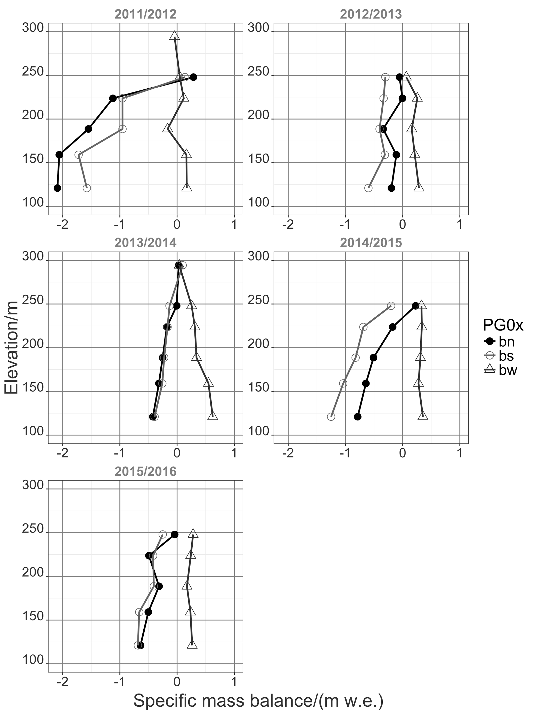
Figure 12Specific summer, winter and net mass balance (bs, bn and bn, respectively) in m w.e. derived from mass balance stakes observation at transects PG0x during 2010 to 2016.
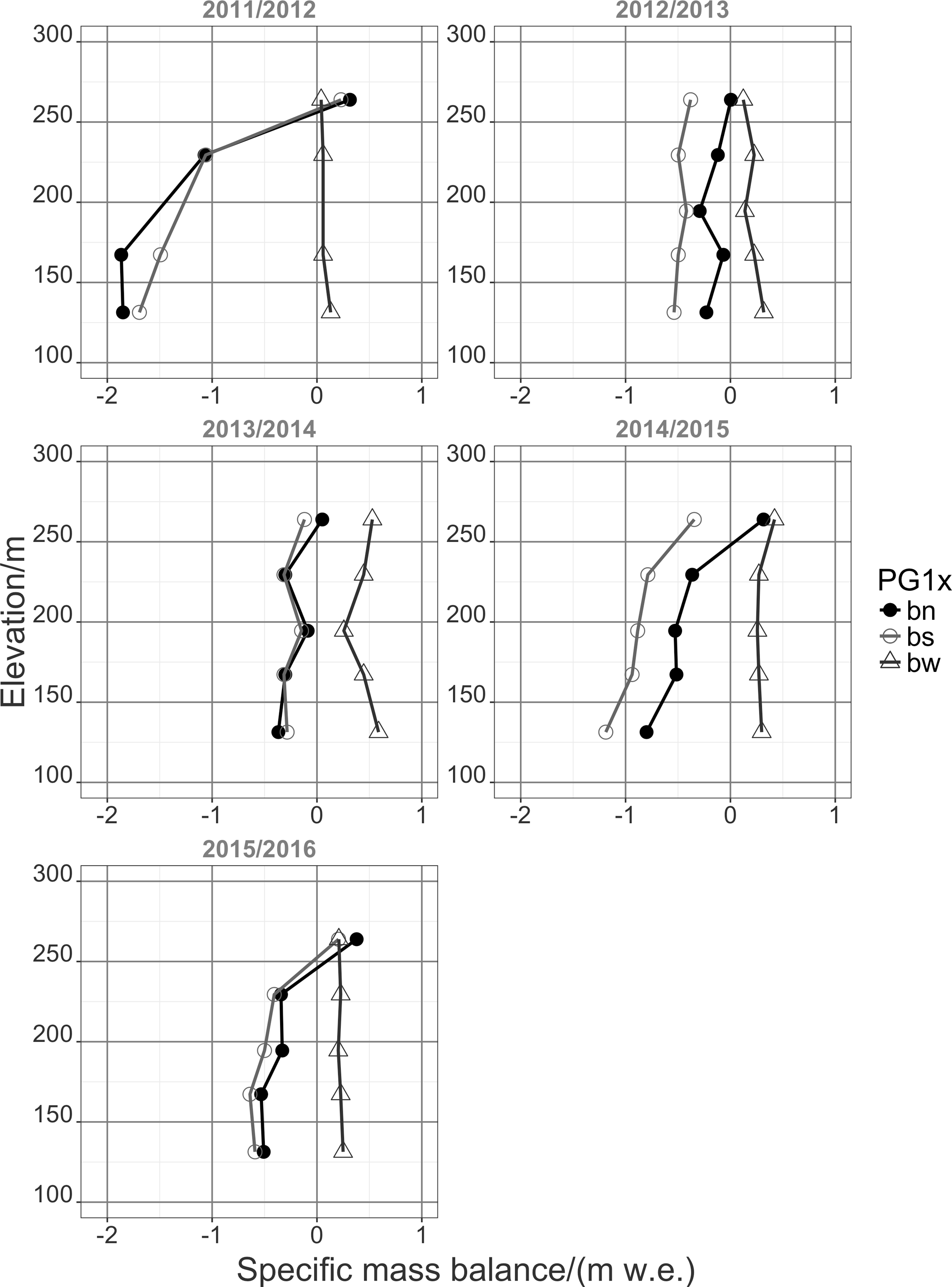
Figure 13Specific summer, winter and net mass balance (bs, bw and bn, respectively) in m w.e. derived from mass balance stakes observation at transect PG1x during 2010 to 2016.
The glaciological year 2011/12 contained a very cold and dry winter in 2011. The summer 2012 showed an exceptionally high net radiation balance amounting to 156 % of the seasonal 5-year average. The resulting high ablation entails a strongly negative specific net balance. In July of winter 2012 brought a 2-week period of rain together with above freezing air temperatures, leading to the erosion of the fresh snow pack and to low accumulation in the net balance. Although the summer 2013 showed low ablation due to high cloud coverage and less precipitation, the glaciological year 2012/13 remains in its net balance negative. It was also a year with very low winds during summer and very high winds during winter. The glaciological year 2013/14 reveals a wet winter with high accumulation rates but also a very cold and very wet summer resulting in low ablation. Regardless of this, the net balance was negative. The glaciological year 2014/15 started with a warm and wet winter, followed by a warm and dry summer leading to higher ablation rates. The period of 2015/16 was a very strong El Niño year with a very cold winter in 2015, followed by a warm and very long summer in 2016. The MSB PG19 (at the elevation of ca. 100 m) clearly reflects the effect of turbulence-driven snow accumulation at the glacier end moraine. Estimates of bn are significantly higher than the GMM output for this stake location. The variability and impact of snow drift and turbulence-driven snow deposition is evident in the locally calculated estimates of bn of the MBS observations. From the graphs (Figs. 12 and 13), it becomes clear that winter accumulation is in most of the years not sufficient to cover for the summer ablation. Summer ablation or the specific summer mass balance, in contrast, is revealed to be highly variable between years, depending on climatic conditions and the length of the ablation period of the respective glaciological year.

Figure 14Time series of meltwater discharge from GMM run November 2010 to November 2015 for the Fourcade Glacier, catchment of the Potter Cove, separated into the different source areas (AID) of snow, firn, ice and rock terrain ( and qrock). The complete simulated meltwater discharge (qcalc) is shown in black solid circle with the standard deviation of the time series in grey envelope.
4.3 Meltwater discharge into Potter Cove
The GMM calculates the discharge on an hourly basis according to the temporal resolution of the meteorological input time series. The GMM configuration allows for computation of partly glaciated catchment areas as is the case for the Potter Cove catchment. The GMM differentiates between the source areas of the meltwater discharge:
Figure 14 shows the temporal evolution of the total meltwater discharge from the complete Potter Cove catchment (qsim) and the respective source areas (firn, ice, snow and rock). The penetration and discharge through ground is negligible, qground≈0. Area sizes change over the course of a year. Figure 14 shows the transitional importance of the dominating source area to glacial discharge throughout the seasons. The contribution of firn areas to glacial discharge is mainly controlled by the seasonal course of surface air temperature and net radiation balance. Since the albedo for firn areas remain high during the summer (α>0.75), firn surface melt starts in spring and consistently pertains throughout the summer with monthly discharge quantities of . The glaciological year 2014/15 contained a very cold and moderately wet winter followed by a very warm but dry summer. This resulted in a pronounced time lag between snow and ice area contribution to glacial discharge but also high meltwater quantities due to the amount of winter precipitation. Glacial discharge from snow areas predominate the first part of a summer season and from ice areas in the second part. Differences in monthly discharge from snow areas can amount to nearly 1 m3 s−1 between years. The high variability of ablation and accumulation reflects the very high inter- and intra-annual variability of the meteorological boundary conditions (Falk and Sala, 2015a). The frequent occurrence of melt periods during winter is attributed to advection of moist and warm air masses from mid-latitudes by synoptic low-pressure systems. This results in non-zero discharge for winter season (JJA: June to August). Figure 15 shows the seasonal sums of glacial discharge from Fourcade Glacier into Potter Cove as sums.

Figure 15Seasonal meltwater discharge from GMM run for the Fourcade Glacier, a hydrological catchment of the Potter Cove (DJF: austral summer December–February; MAM: austral fall March–May; JJA: austral winter June–August; SON: austral spring September–November).
Linearly relating the time series of simulated discharge to the positive degree day (PDD) time series derived from the Carlini air temperature series (Falk and Sala, 2015a) shows a high correlation coefficient:
This means that 84 % of the changes in discharge can be explained by changes in air temperature. Observed temperature trends are highest in winter months, i.e. a trend in minimum air temperature of nearly 5 ∘C over four decades for August (Falk and Sala, 2015a). This might result in lesser accumulation during winter and, thus, in a more negative mass balance. The linear regression between the simulated discharge to the PDD time series calculated from the AWS data shows a lesser correlation:
Above glaciated areas, surface air temperature is being reduced by the melt processes. Thus, PDD and degree day factor analysis are best derived from air temperature observations that are within the catchment area but on non-glaciated areas.

Figure 16Equilibrium line altitude calculated from observations at transects PG0x (black, solid circle) and PG1x (black, solid triangle) and from GMM simulation (M) output at transects pixels PG0x (red, solid circle) and PG1x (red, solid triangle) for the time period 2010 to 2016. The 5-year average ELA from MBS observations (MBS obs) and from GMM model results (GMM) are displayed with the grey shading indicating the uncertainty around the average observed ELA.
The observed trend in SAM and surface air temperature especially during wintertime (Falk and Sala, 2015a) can lead to significant glacial discharge within the winter season. Glacier facies with bare-ice conditions promote enhanced glacial discharge (see Fig. 14). The dark material, periodically resurfacing in the ablation area, significantly changes albedo to values α<0.1 and, thus, reinforces the effect on surface melt. Hence, winters with missing or lesser accumulation can be expected to be followed by summers with higher rates of glacier discharge.
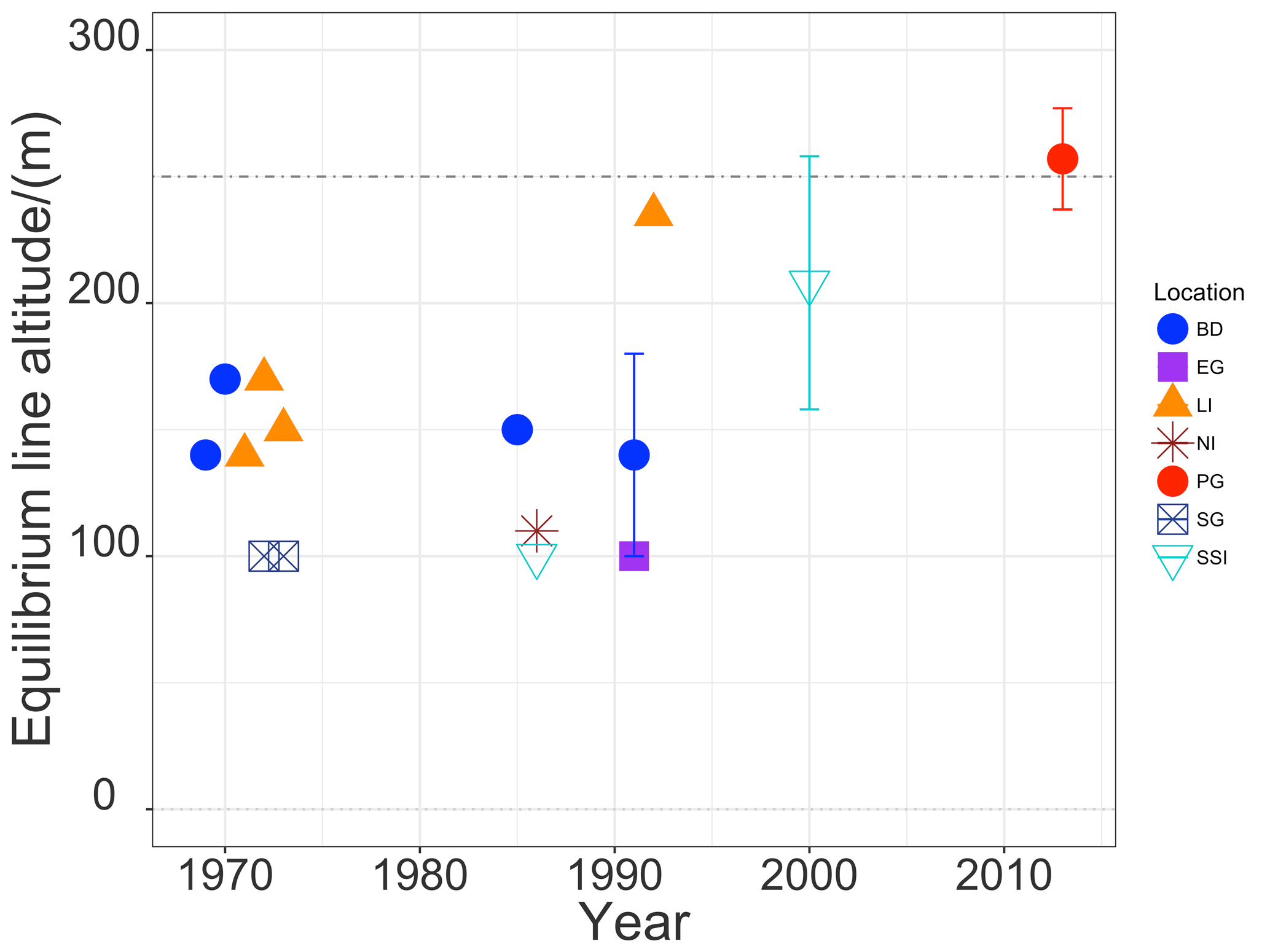
Figure 17Equilibrium line altitude estimates from this study (PG) and former glaciological studies during the last decades. ELA estimates taken from literature encompass: BD is Bellingshausen Dome, KGI (Jiahong et al., 1994; Jiawen et al., 1995; Orheim and Govorukha, 1982); EG is Ecology Glacier, KGI (Bintanja, 1995); LI is Livingston Island (Molina et al., 2007; Navarro et al., 2009, 2013; Vilaplana and Pallàs, 1994); NI is Nelson Island (Jiawen et al., 1995); SG is Stenhouse Glacier, KGI (Curl, 1980); SSI is South Shetland Islands (Serrano and López-Martínez, 2000).
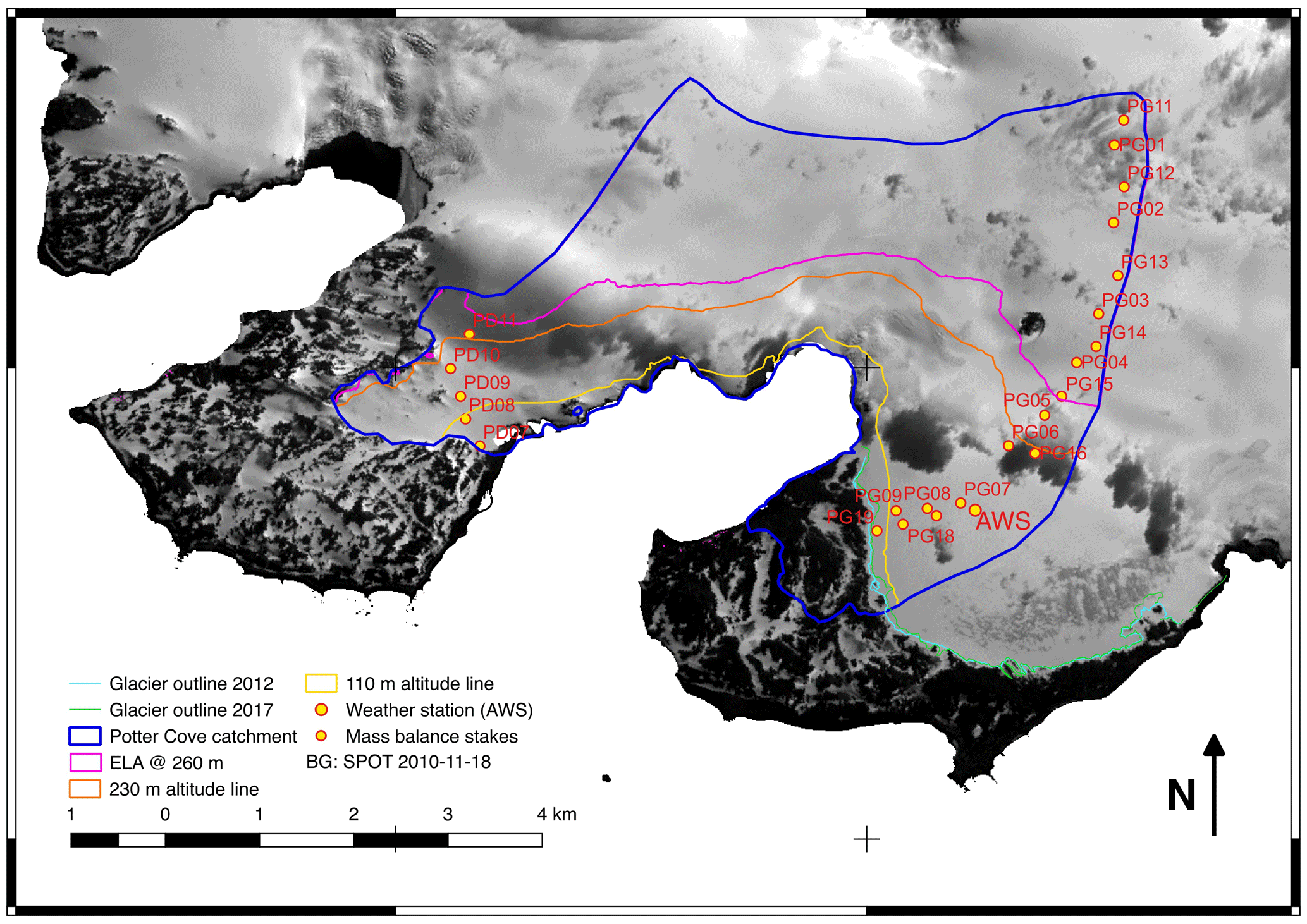
Figure 18Glacier extent for equilibrium with actual climatic boundary conditions and an ELA of 260 m (pink line) for the Potter Cove catchment on KGI, according to an AAR between 0.5 (yellow line) and 0.8 (orange line). The actual glacier extent is marked as green and light blue line and represents our own differential GPS measurements in austral summer 2012/13 and 2016/17.
Time series of accumulation and ablation show a very high intra- and interannual variability that concurs with the climatological variability that is reported by Falk and Sala (2015a). The observations at two mass balance stake transects demonstrate the high spatial variability, regular occurrence of winter melt periods and the impact of snow drift, turbulence-driven snow deposition, snow layer erosion by rain and high exposition to synoptic impact. These processes are not yet included in the model physics and can lead to discrepancies between GMM simulation and observations under specific climatic conditions. Overall, observations and model are in good agreement though. The high interannual variability in climate conditions, accumulation and ablation patterns is propagated to variability in glacial discharge time series. The difference between years can be as high as 40 %. The simulated glacier discharge is highly correlated to PDD time series with a coefficient of determination of R2=0.84.
The ELA is defined as a set of points on a glacier surface where the climatic mass balance is zero (Cogley et al., 2011), thus separating accumulation from ablation area. The ELA conveys an instantaneous response to the climatic boundary conditions. The AAR is the ratio of accumulation area to total glacier surface area and defines the boundaries of the glacier in equilibrium state with its climatic boundary conditions. The expected future extent of the ice cap of the Fourcade will be assessed by the AAR in the conclusions.
Figure 16 shows the ELA estimates from observations (black) at the transects PG1x and PG0x and from the GMM output (red). Error bars are derived from the regressions. The calculated ELAs are generally around 260 m altitude. Curl (1980) states that all glaciers on KGI appear in near-equilibrium and slightly negative conditions and that geological evidence shows no major detectable advance within the past two centuries. Braun and Gossmann (2002) have compiled values of the ELA obtained by different authors in the South Shetland Islands region along the last decades. Jiawen et al. (1995) do not give uncertainties of their glaciological observations and ELA estimates but state that a high variability between different consecutive years was observed. Jiahong et al. (1994) and Jiahong et al. (1998) concluded from mass balance studies on Collins or Bellingshausen Dome that this small ice cap was in steady state between 1971 and 1991 in agreement with Curl (1980). Serrano and López-Martínez (2000) presented a concurrent ELA for the South Shetland Islands located around 165 to 250 Bintanja (1995) asserted that the ELA was around 100 m in the Ecology Glacier, KGI. Despite the strong variability, the ELA has increased by more than 100 m from the late 1960s up to the 1990s. More recently Osmanoglu et al. (2014), Navarro et al. (2009, 2013) and Molina et al. (2007) have placed the ELA at ∼230 m and ∼187 m for Hurd and Johnsons glaciers, respectively, both located at Livingston Island ice cap.
Until recently, the remote sensing data from synthetic aperture radar (SAR) measurements only allowed for analysis during the summer months due to seasonal manning of the Chilean base O'Higgins responsible for the download of data from the overpassing satellite, thus only resulting in the estimation of the transient snow line, in this case the firn line. Hence, the ELA would be systematically underestimated during a negative surface mass balance year. Additionally, SAR data were not corrected for incidental angles, thus not allowing for differentiation of ablation patterns from superimposed ice. The ELA analysis here is based on ground-based glaciological studies only, and remote sensing studies have been disregarded to avoid methodological bias in the ELA analysis. Multi-temporal SAR data analysis carried out by Falk et al. (2016) resulted in an ELA of ca. 250 m for the glaciological year 2010/11 during a cold and snowy summer. Field observations support the importance of snow drift on the accumulation patterns due to the high wind speeds and the related snow drift and accumulation according to domes and troughs. The average ELA was derived from our own glaciological studies on KGI over the time period 2010–2015 to 260±20 m and is displayed in Fig. 16 as a dot-dashed line with the uncertainty in grey shading.
Figure 17 places the results from our own glaciological observations into the long-term context. Where available, error or uncertainty bars were included. The temporal evolution of the ELA estimates from the different glaciological studies show clearly that until the 1980s the glaciers on KGI were in near-equilibrium (Curl, 1980), but after this time period there is a clear increase in the ELA. Our analysis in the preceding paragraphs shows not only that the accumulation of Fourcade Glacier generally does not suffice to account for the ablation but also that the interannual variability is high especially during the ablation period. The Fourcade Glacier is clearly in retreating mode, also due to the fact that ice flow velocities in lower glacier on Potter Peninsula are below 1 m yr−1 (Falk et al., 2016). The ice mass flux cannot compensate the melt losses in the ablation zone.
The expected ratio of accumulation area to the total glacierized area for a glacier in equilibrium with its climate (AAReq) is within the range of 0.5 to 0.8, e.g. Meier and Post (1962) and Paterson (1994). Corresponding to the observed average ELA of 260 m with concurrent glacier extent is a ratio of approx. 0.26 for the Potter Cove catchment, meaning the glacier is clearly retreating until it reaches its equilibrium state shown in Fig. 18. Here, the yellow line marks the glacier extent for elevations above 110 m referring to an AAR=0.8 and the orange line marks the glacier extent for elevations above 230 m referring to an AAR of 0.5. Underlying is the assumption that lower elevations will melt homogeneously and ice velocities are negligible as soon as the glacier terminates on land in the Potter Cove catchment.
One of the most intuitive parameters to describe the equilibrium state of a glacier is the AAR, meaning the state and health of a glacier. Particularly, it is an indicator for expected future retreat or growth of a glacier until it gets into equilibrium with concurrent climatic conditions. It thus relates via the ELA with the specific mass balance and changes of total glacier area. The more negative the mass balance, the higher the elevation line of ELA and the smaller the AAR. Once the long-term ELA reaches values higher than the maximum altitude of the glacier dome, there is no more accumulation area and the glacier will disappear sooner or later. Möller and Schneider (2015) define this as the turning or tipping point of the glacier evolution.
This behaviour also depends on the bedrock topography, which remains largely unknown for the Warszawa Icefield. If underneath the glacier is mountainous terrain, then the stratigraphy of glacier ice mass would persist longer due to higher elevation than if it would all be ice mass underneath. Glaciers respond to climatic boundary conditions with a time lag of a few decades to centuries until they are in equilibrium with the climatic conditions (Paterson, 1994). The already committed mass change will lead to further retreat of the glacier border within the near future.
A tipping point will be reached for the glacier when the ELA rises above the highest point of the glacier which implies that the accumulation area goes to zero, i.e. an ELA>490 m. Even if the observed trends in climatic boundary conditions do not continue, the Fourcade Glacier would still retreat until it reaches equilibrium with climatic conditions. Its extent will be defined by these conditions and the glacier border located between the yellow and the orange line in Fig. 18. The equilibrium state corresponds to a glacier extent that would approximately end between the elevation lines of helev=110 m (Fig. 18 yellow line) and helev=230 m (Fig. 18 orange line), referring to an AAReq of 0.8 and of 0.5, respectively. Thus, further retreat of the glacier border is to be expected. The southern part of the Fourcade Glacier on Potter and on Barton Peninsula contains a major area of very low ice flow velocities <1 m2 and below the ELA in the ablation zone. These areas can be assumed to decrease the most and the glacial meltwater streams are likely to significantly increase their sediment freight due to larger distances through moraine landscape.
The high variability in melt conditions and in especially missing winter accumulation is found to enhance glacial discharge. Positive air temperatures and thus non-frozen moraine landscape surface also promote the intake of sediment load into the meltwater streams that is then introduced into the coastal waters. Assuming the most extreme scenario of glacial retreat according to the ELA–AAR analysis (Fig. 18), the length of meltwater streams through moraine landscape could increase by as much as three times the current stream length, expecting to pick up more sediment load in the near future. This would increase changes in physical and chemical properties of coastal environments, hence leading to a higher impact on the biological communities. Considering the high adaptation required for Antarctica's extreme environments, the high seasonal and interannual variability in climatic and glacial melting conditions can be assumed to have a direct impact on coastal ecosystems.
All R codes are available on request from Ulrike Falk.
Supplementary data are available at https://doi.org/10.1594/PANGAEA.874599 (Falk et al., 2017) and https://doi.org/10.1594/PANGAEA.848704 (Falk and Sala, 2015b).
UF was the PI of the glaciological and climatological work package within the IMCOAST project and also led the glaciological modelling work on KGI within the IMCONet project. DL was responsible for the quality assessment and control of mass balance data time series, the establishment of final glaciological protocols and all communication with the overwinterers. All final analysis and post-processing of climatological and glaciological data time series was performed by UF. ASB investigated the hydrology of Potter Cove and refined the catchment definition grids for the glaciological surface mass balance model. Glaciological modelling work was carried out by UF, with ASB contributing to the calibration and validation procedures. The manuscript was mainly written by UF. DL contributed to the sections concerning mass balance stake observations and analysis, as well as glacier mass balance. ASB wrote parts for the hydrological catchment definition and contributed to the sections on glacier discharge and meltwater analysis.
There are no potential conflicts of interest regarding financial, political or other matters.
We would like to thank the Alfred Wegener Institute (AWI) from Germany and
the Instituto Antártico Argentino – Dirección Nacional del Antártico
(IAA-DNA) from Argentina for their support in Antarctica. A special
acknowledgement goes to Hernán Sala for assistance in the field and help
with logistics and to the overwintering scientists at Carlini Station and
Dallmann Laboratory: Daniel Viqueira, Juan Piscicelli, Facundo Alvarez,
Francisco Ferrer, Pablo Saibene, Martín Gingins and Julia Luna without whom
this work would not have been possible. During the period 2010–2015, the
overwintering crews from the Ejército Argentino at Carlini Station
continuously supported our scientific tasks and we would like to specifically
mention SP Norberto Leonardo Galván. We also than Regine Hoch and the
University of Fairbanks in Alaska for the introduction to the glacier melt
model. All graphs in this paper were produced using the R programming
language (R Core Team, 2014) and QGIS software (QGIS Development Team, 2016). We also thank the
funding support provided by the ESF ERANET Europolar IMCOAST project (BMBF
award AZ 03F0617B) and the Marie Curie Action IRSES (FP7 IRSES, action no.
318718), the logistic support by the Universities of Bonn, Bremen and
Erlangen-Nuremberg and the Argentinean Antarctic Institute (IAA-DNA). We
thank Ben Marzeion for the careful reading of and his very helpful comments
on the manuscript.
The article processing
charges for this open-access
publication were covered by the
University of Bremen.
Edited by: Thomas
Mölg
Reviewed by: two anonymous referees
AARI: Meteorological observations at Bellingshausen, Arctic and Antarctic Research Institute, St. Petersburg, Russia, available at: http://www.aari.nw.ru/index_en.html, last access: 1 January 2016. a
Abele, D., Vazquez, S., Buma, A., Hernandez, E., Quiroga, C., Held, C., Frickenhaus, S., Harms, L., Lopez, J., Helmke, E., and Mac Cormack, W. P.: Pelagic and benthic communities of the Antarctic ecosystem of Potter Cove: Genomics and ecological implications, Mar. Genom., 33, 1–11, https://doi.org/10.1016/j.margen.2017.05.001, 2017. a
Abram, N., Thomas, E. R., McConnell, J. R., Mulvaney, R., Bracegirdle, T. J., Sime, L. C., and Aristarain, A.: Ice core evidence for a 20th century decline of sea ice in the Bellingshausen Sea, Antarctica, J. Geophys. Res., 115, 9, https://doi.org/10.1029/2010JD014644, 2010. a
Andreas, E.: IA theory for the scalar roughness and the scalar transfer coefficients over snow and sea ice, Bound.-Lay. Meteorol., 38, 159–184, 1987. a
Barrand, N., Vaughan, D., Steiner, N., Tedesco, M., Kuipers Munneke, P., Broeke, M., and Hosking, J.: Trends in Antarctic Peninsula surface melting conditions from observations and regional climate modeling, J. Geophys. Res.-Earth, 118, 315–330, 2013. a, b
Bintanja, R.: The local surface energy balance of the Ecology Glacier, King George Island, Antarctica: measurements and modelling, Antarct. Sci., 7, 315–325, https://doi.org/10.1017/S0954102095000435, 1995. a, b
Birkenmajer, K.: Retreat of Ecology Glacier, Admiralty Bay, King George Island (South Shetland Islands, West Antarctica), 1956–2001, B. Pol. Acad. Sci.-Earth, 50, 15–29, 2002. a
Bishop, M. P., Olsenholler, J. A., Shroder, J. F., Barry, R. G., Raup, B. H., Bush, A. B., Copland, L., Dwyer, J. L., Fountain, A. G., Haeberli, W., Kääb, A., Paul, F., Hall, D. K., Kargel, J. D., Molnia, B. F., Trabant, D. C., and Wessels, R.: Global Land Ice Measurements from Space (GLIMS): remote sensing and GIS investigations of the Earth's cryosphere, Geocarto Int., 19, 57–84, 2004. a
Braun, M. and Gossmann, H.: Glacial Changes in the Areas of Admiralty Bay and Potter Cove, King George Island, Maritime Antarctica, Springer, Berlin Heidelberg, 75–89, 2002. a, b
Braun, M. and Hock, R.: Spatially distributed surface energy balance and ablation modelling on the ice cap of King George Island (Antarctica), Global Planet. Change, 42, 45–58, 2004. a, b
Braun, M., Humbert, A., and Moll, A.: Changes of Wilkins Ice Shelf over the past 15 years and inferences on its stability, The Cryosphere, 3, 41–56, https://doi.org/10.5194/tc-3-41-2009, 2009. a, b
Braun, M., Betsch, T., and Seehaus, T.: King George Island TanDEM-X DEM, link to GeoTIFF, Geographic Institute, Universitaet Erlangen-Nuernberg, https://doi.org/10.1594/PANGAEA.863567, 2016. a, b
Brock, B. W., Willis, I. C., and Sharp, M. J.: Measurement and parameterization of aerodynamic roughness length variations at Haut Glacier d'Arolla, Switzerland, J. Glaciol., 52, 281–297, 2006. a
Bromwich, D. H., Rogers, A. N., Kållberg, P., Cullather, R. I., White, J. W., and Kreutz, K. J.: ECMWF analyses and reanalyses depiction of ENSO signal in Antarctic precipitation, J. Climate, 13, 1406–1420, 2000. a
Campbell, G. S. and Norman, J. M.: Environmental Biophysics, 2nd Edn., Springer, New York, Berlin, Heidelberg, 2000. a
Cape, M. R., Vernet, M., Skvarca, P., Marinsek, S., Scambos, T., and Domack, E.: Foehn winds link climate-driven warming to ice shelf evolution in Antarctica, J. Geophys. Res.-Atmos., 120, 11037–11057, https://doi.org/10.1002/2015JD023465, 2015. a
Chapman, W. L. and Walsh, J. E.: A synthesis of Antarctic temperatures, J. Climate, 20, 4096–4117, 2007. a
Clarke, A., Murphy, E. J., Meredith, M. P., King, J. C., Peck, L. S., Barnes, D. K., and Smith, R. C.: Climate change and the marine ecosystem of the western Antarctic Peninsula, Philos. T. Roy. Soc. B, 362, 149–166, 2007. a
Cogley, J., Hock, R., Rasmussen, L., Arendt, A., Bauder, A., Braithwaite, R., Jansson, P., Kaser, G., Möller, M., Nicholson, L., and Zemp, M.: Glossary of glacier mass balance and related terms, IHP-VII technical documents in hydrology No. 86, IACS Contribution No. 2, 2011. a, b
Cook, A., Fox, A., Vaughan, D., and Ferrigno, J.: Retreating glacier fronts on the Antarctic Peninsula over the past half-century, Science, 308, 541–544, 2005. a
Curl, J. E.: A glacial history of the South Shetland Islands, Antarctica, Tech. rep., Institute of Polar Studies, The Ohio State University, 1980. a, b, c
Davis, C. H., Li, Y., McConnell, J. R., Frey, M. M., and Hanna, E.: Snowfall-driven growth in East Antarctic ice sheet mitigates recent sea-level rise, Science, 308, 1898–1901, 2005. a
De Angelis, H. and Skvarca, P.: Glacier surge after ice shelf collapse, Science, 299, 1560–1562, 2003. a
Doran, P. T., Priscu, J. C., Lyons, W. B., Walsh, J. E., Fountain, A. G., McKnight, D. M., Moorhead, D. L., Virginia, R. A., Wall, D. H., Clow, G. D., and Fritson, C. H.: Antarctic climate cooling and terrestrial ecosystem response, Nature, 415, 517–520, 2002. a
Ducklow, H. W., Baker, K., Martinson, D. G., Quetin, L. B., Ross, R. M., Smith, R. C., Stammerjohn, S. E., Vernet, M., and Fraser, W.: Marine pelagic ecosystems: the west Antarctic Peninsula, Philos. T. Roy. Soc. B, 362, 67–94, 2007. a
Eraso, A., and Domínguez, M.: Physicochemical characteristics of the subglacier discharge in Potter Cove, King George Island, Antarctica, Karst and Cryokarst, 45, 111–122, 2007. a
Fahnestock, M. A., Abdalati, W., and Shuman, C. A.: Long melt seasons on ice shelves of the Antarctic Peninsula: an analysis using satellite-based microwave emission measurements, Ann. Glaciol., 34, 127–133, 2002. a
Falk, U. and Sala, H.: Winter melt conditions of the inland ice cap of King George Island, Antarctic Peninsula, Erdkunde, 341–363, 2015a. a, b, c, d, e, f, g, h, i, j, k, l, m, n, o, p, q, r
Falk, U. and Sala, H.: Continuous meteorological observations at station ZAWS, Warszawa Icefield, King George Island, Antarctic Peninsula, 2012-01, PANGAEA, https://doi.org/10.1594/PANGAEA.848704, 2015b. a
Falk, U., Gieseke, H., Kotzur, F., and Braun, M.: Monitoring snow and ice surfaces on King George Island, Antarctic Peninsula, with high-resolution TerraSAR-X time series, Antarct. Sci., 28, 135–149, 2016. a, b, c, d
Falk, U., López, D., and Silva-Busso, A. A.: Recent changes in glacier mass balance and equilibrium line altitude and the impact of climatic change on King George Island, Antarctic Peninsula, PANGAEA, https://doi.org/10.1594/PANGAEA.874599, 2017. a
Ferron, F. A., Simões, J. C., Aquino, F. E., and Setzer, A. W.: Air temperature time series for King George Island, Antarctica, Pesquisa Antártica Brasileira, 4, 155–169, 2004. a
Fogt, R. L. and Zbacnik, E. A.: Sensitivity of the Amundsen Sea low to stratospheric ozone depletion, J. Climate, 27, 9383–9400, 2014. a
Gates, D. M.: Biophysical Ecology, Springer, New York, 611 pp., 1980. a
Heinemann, G. and Falk, U.: Surface winds and energy fluxes near the Greenland ice margin under conditions of katabatic winds, Polarforschung, 71, 15–31, 2002. a
Henkel, S., Kasten, S., Sala, H., Busso, A. S., and Staubwasser, M.: Effect of increased glacier melt on diagenetic Fe cycling in marine sediments at King George Island (Antarctica), Mineral. Mag. H: Goldschmidt Abstracts 2013, 77, 1287–1287, 2013. a
Hock, R. and Holmgren, B.: A distributed surface energy-balance model for complex topography and its application to Storglaciären, Sweden, J. Glaciol., 51, 25–36, 2005. a
Jiahong, W., Jiancheng, K., Jiankang, H., Zichu, X., and Lluberas, A.: Climate, mass balance and glacial changes on small dome of Collins Ice Cap, King George Island, Antarctica, Antarct. Res., 5, 52–61, 1994. a, b
Jiahong, W., Jiancheng, K., Jiankang, H., Zichu, X., Leibao, L., and Dali, W.: Glaciological studies on the King George Island ice cap, South Shetland Islands, Antarctica, Ann. Glaciol., 27, 105–109, 1998. a, b
Jiawen, R., Dahe, Q., Petit, J., Jouzel, J., Wenti, W., Chen, L., Xiaojun, W., Songlin, Q., and Xiaoxiang, W.: Glaciological studies on Nelson Island, South Shetland Islands, Antarctica, J. Glaciol., 41, 408–412, 1995. a, b, c
Joughin, I., Smith, B. E., and Medley, B.: Marine ice sheet collapse potentially under way for the Thwaites Glacier Basin, West Antarctica, Science, 344, 735–738, 2014. a
Martianov, V. and Rakusa-Suszczewski, S.: Ten years of climate observations at the Arctowski and Bellingshausen stations (King George Is., South Shetlands, Antarctica), Global change, regional research centres, 80–87, 1989. a
Meier, M. F. and Post, A.: Recent variations in mass net budgets of glaciers in western North America, in: Symposium at Obergurgl 1962 Variations of Glaciers, 1962. a
Meredith, M. P. and King, J. C.: Rapid climate change in the ocean west of the Antarctic Peninsula during the second half of the 20th century, Geophys. Res. Lett., 32, L19604, https://doi.org/10.1029/2005GL024042, 2005. a
Meredith, M. P., Renfrew, I. A., Clarke, A., King, J. C., and Brandon, M. A.: Impact of the 1997/98 ENSO on upper ocean characteristics in Marguerite Bay, western Antarctic Peninsula, J. Geophys. Res.-Oceans, 109, C09013, https://doi.org/10.1029/2003JC001784, 2004. a
Molina, C., Navarro, F., Calvet, J., García-Sellés, D., and Lapazaran, J.: Hurd Peninsula glaciers, Livingston Island, Antarctica, as indicators of regional warming: ice-volume changes during the period 1956–2000, Ann. Glaciol., 46, 43–49, 2007. a, b
Möller, M., and Schneider, C.: Temporal constraints on future accumulation-area loss of a major Arctic ice cap due to climate change (Vestfonna, Svalbard), Sci. Rep.-UK, 5, 8079, https://doi.org/10.1038/srep08079, 2015. a
Monteith, J. and Unsworth, M.: Principles of environmental physics, Arnold, London, 1990. a
Montes-Hugo, M., Doney, S. C., Ducklow, H. W., Fraser, W., Martinson, D., Stammerjohn, S. E., and Schofield, O.: Recent changes in phytoplankton communities associated with rapid regional climate change along the western Antarctic Peninsula, Science, 323, 1470–1473, 2009. a
Navarro, F., Otero, J., Macheret, Y., Vasilenko, E., Lapazaran, J., Ahlstrøm, A., and Machio, F.: Radioglaciological studies on Hurd Peninsula glaciers, Livingston Island, Antarctica, Ann. Glaciol., 50, 17–24, 2009. a, b
Navarro, F. J., Jonsell, U. Y., Corcuera, M. I., and Martín-Español, A.: Decelerated mass loss of Hurd and Johnsons Glaciers, Livingston Island, Antarctic Peninsula, J. Glaciol., 59, 115–128, 2013. a, b
Orheim, O. and Govorukha, L.: Present-day glaciation in the South Shetland Islands, Ann. Glaciol., 3, 233–238, 1982. a, b
Orr, A., Marshall, G. J., Hunt, J. C., Sommeria, J., Wang, C.-G., Van Lipzig, N. P., Cresswell, D., and King, J. C.: Characteristics of summer airflow over the Antarctic Peninsula in response to recent strengthening of westerly circumpolar winds, J. Atmos. Sci., 65, 1396–1413, 2008. a
Osmanoglu, B., Navarro, F. J., Hock, R., Braun, M., and Corcuera, M. I.: Surface velocity and mass balance of Livingston Island ice cap, Antarctica, The Cryosphere, 8, 1807–1823, https://doi.org/10.5194/tc-8-1807-2014, 2014. a
Parish, T. R. and Bromwich, D. H.: Reexamination of the near-surface airflow over the Antarctic continent and implications on atmospheric circulations at high southern latitudes, Mon. Weather Rev., 135, 1961–1973, 2007. a
Parkinson, C. L.: Trends in the length of the Southern Ocean sea-ice season, 1979–1999, Ann. Glaciol., 34, 435–440, 2002. a
Paterson, W.: The physics of glaciers, 480 pp., 1994. a, b
Payne, A. J., Vieli, A., Shepherd, A. P., Wingham, D. J., and Rignot, E.: Recent dramatic thinning of largest West Antarctic ice stream triggered by oceans, Geophys. Res. Lett., 31, L23401, https://doi.org/10.1029/2004GL021284, 2004. a
Peck, L. S., Webb, K. E., and Bailey, D. M.: Extreme sensitivity of biological function to temperature in Antarctic marine species, Funct. Ecol., 18, 625–630, 2004. a
Perlwitz, J., Pawson, S., Fogt, R. L., Nielsen, J. E., and Neff, W. D.: Impact of stratospheric ozone hole recovery on Antarctic climate, Geophys. Res. Lett., 35, L08714, https://doi.org/10.1029/2008GL033317, 2008. a
Pfeffer, W. T., Arendt, A. A., Bliss, A., Bolch, T., Cogley, J. G., Gardner, A. S., Hagen, J.-O., Hock, R., Kaser, G., Kienholz, C., Miles, E. S., Moholdt, G., Mölg, N., Paul, F., Radić, V., Rastner, P., Raup, B. H., Rich, J., Sharp, M. J., and The Randolph Consortium: The Randolph Glacier Inventory: a globally complete inventory of glaciers, J. Glaciol., 60, 537–552, 2014. a
QGIS Development Team: QGIS Geographic Information System, available at: http://www.qgis.org (last access: 1 May 2017), 2016. a
Quartino, M. L., Deregibus, D., Campana, G. L., Latorre, G. E. J., and Momo, F. R.: Evidence of macroalgal colonization on newly ice-free areas following glacial retreat in Potter Cove (South Shetland Islands), Antarctica, PLoS One, 8, e58223, https://doi.org/10.1371/journal.pone.0058223, 2013. a
R Core Team: R: A language and environment for statistical computing, available at: http://www.R-project.org (last access: 31 August 2017), 2014. a
Rau, F., Mauz, F., de Angelis, H., Jaña, R., Neto, J. A., Skvarca, P., Vogt, S., Saurer, H., and Gossmann, H.: Variations of glacier frontal positions on the northern Antarctic Peninsula, Ann. Glaciol., 39, 525–530, 2004. a
Reijmer, C. and Hock, R.: A distributed energy balance model including a multi-layer sub-surface snow model, J. Glaciol., 54, 61–72, 2008. a, b
Rignot, E., Mouginot, J., and Scheuchl, B.: Antarctic grounding line mapping from differential satellite radar interferometry, Geophys. Res. Lett., 38, L10504, https://doi.org/10.1029/2011GL047109, 2011. a
Rott, H., Skvarca, P., and Nagler, T.: Rapid collapse of northern Larsen ice shelf, Antarctica, Science, 271, 788–792, https://doi.org/10.1126/science.271.5250.788, 1996. a
Rückamp, M. and Blindow, N.: King George Island ice cap geometry updated with airborne GPR measurements, Earth Syst. Sci. Data, 4, 23–30, https://doi.org/10.5194/essd-4-23-2012, 2012. a
Rückamp, M., Braun, M., Suckro, S., and Blindow, N.: Observed glacial changes on the King George Island ice cap, Antarctica, in the last decade, Global Planet. Change, 79, 99–109, 2011. a, b, c, d
Scambos, T., Ross, R., Bauer, R., Yermolin, Y., Skvarca, P., Long, D., Bohlander, J., and Haran, T.: Calving and ice-shelf break-up processes investigated by proxy: Antarctic tabular iceberg evolution during northward drift, J. Glaciol., 54, 579–591, 2008. a
Scambos, T. A., Hulbe, C., Fahnestock, M., and Bohlander, J.: The link between climate warming and break-up of ice shelves in the Antarctic Peninsula, J. Glaciol., 46, 516–530, 2000. a
Schloss, I. R., Abele, D., Moreau, S., Demers, S., Bers, A. V., González, O., and Ferreyra, G. A.: Response of phytoplankton dynamics to 19-year (1991–2009) climate trends in Potter Cove (Antarctica), J. Marine Syst., 92, 53–66, 2012. a
Serrano, E., and López-Martínez, J.: Rock glaciers in the South Shetland Islands, Western Antarctica, Geomorphology, 35, 145–162, 2000. a, b
Shepherd, A., Wingham, D., Payne, T., and Skvarca, P.: Larsen ice shelf has progressively thinned, Science, 302, 856–859, 2003. a
Sherrell, R., Lagerström, M., Forsch, K., Stammerjohn, S., and Yager, P.: Dynamics of dissolved iron and other bioactive trace metals (Mn, Ni, Cu, Zn) in the Amundsen Sea Polynya, Antarctica, Elementa, 3, 000071, https://doi.org/10.12952/journal.elementa.000071, 2015. a
Shuman, C. A. and Stearns, C. R.: Decadal-length composite inland West Antarctic temperature records, J. Climate, 14, 1977–1988, 2001. a
Skvarca, P., Rack, W., Rott, H., DonáNgelo, Y., and IbarzáBal, T.: Evidence of recent climatic warming on the eastern Antarctic Peninsula, Ann. Glaciol., 27, 628–632, 1998. a
Skvarca, P., Rack, W., Rott, H., and Donángelo, T. I.: Climatic trend and the retreat and disintegration of ice shelves on the Antarctic Peninsula: an overview, Polar Res., 18, 151–157, 1999. a
Skvarca, P., De Angelis, H., and Zakrajsek, A. F.: Climatic conditions, mass balance and dynamics of Larsen B ice shelf, Antarctic Peninsula, prior to collapse, Ann. Glaciol., 39, 557–562, 2004. a, b
Smeets, C. and Van den Broeke, M.: Temporal and spatial variations of the aerodynamic roughness length in the ablation zone of the Greenland ice sheet, Bound.-Lay. Meteorol., 128, 315–338, 2008. a
Smith, R. C., Ainley, D., Baker, K., Domack, E., Emslie, S., Fraser, B., Kennett, J., Leventer, A., Mosley-Thompson, E., Stammerjohn, S., and Vernet, M.: Marine Ecosystem Sensitivity to Climate Change Historical observations and paleoecological records reveal ecological transitions in the Antarctic Peninsula region, BioScience, 49, 393–404, 1999. a
SMN: Meteorological observations at Carlini base, Argentinean Meteorological Service, Argentina, Buenos Aires, available at: http://www.smn.gov.ar, last access: 1 January 2016. a
Stammerjohn, S., Massom, R., Rind, D., and Martinson, D.: Regions of rapid sea ice change: An inter-hemispheric seasonal comparison, Geophys. Res. Lett., 39, L06501, https://doi.org/10.1029/2012GL050874, 2012. a
Steig, E. J., Schneider, D. P., Rutherford, S. D., Mann, M. E., Comiso, J. C., and Shindell, D. T.: Warming of the Antarctic ice-sheet surface since the 1957 International Geophysical Year, Nature, 457, 459–462, 2009. a, b
Thompson, D. W. and Solomon, S.: Interpretation of recent Southern Hemisphere climate change, Science, 296, 895–899, 2002. a, b
Thompson, D. W., Solomon, S., Kushner, P. J., England, M. H., Grise, K. M., and Karoly, D. J.: Signatures of the Antarctic ozone hole in Southern Hemisphere surface climate change, Nat. Geosci., 4, 741–749, 2011. a
Turner, J.: The El Niño–Southern Oscillation and Antarctica, Int. J. Climatol., 24, 1–31, 2004. a
Turner, J., Colwell, S. R., Marshall, G. J., Lachlan-Cope, T. A., Carleton, A. M., Jones, P. D., Lagun, V., Reid, P. A., and Iagovkina, S.: Antarctic climate change during the last 50 years, Int. J. Climatol., 25, 279–294, 2005. a
Turner, J., Comiso, J. C., Marshall, G. J., Lachlan-Cope, T. A., Bracegirdle, T., Maksym, T., Meredith, M. P., Wang, Z., and Orr, A.: Non-annular atmospheric circulation change induced by stratospheric ozone depletion and its role in the recent increase of Antarctic sea ice extent, Geophys. Res. Lett., 36, L08502, https://doi.org/10.1029/2009GL037524, 2009. a
van den Broeke, M., van As, D., Reijmer, C., and van de Wal, R.: Assessing and improving the quality of unattended radiation observations in Antarctica, J. Atmos. Ocean. Tech., 21, 1417–1431, 2004. a
Van den Broeke, M., Van de Berg, W. J., and Van Meijgaard, E.: Snowfall in coastal West Antarctica much greater than previously assumed, Geophys. Res. Lett., 33, L02505, https://doi.org/10.1029/2005GL025239, 2006. a
Vaughan, D. G., Marshall, G. J., Connolley, W. M., Parkinson, C., Mulvaney, R., Hodgson, D. A., King, J. C., Pudsey, C. J., and Turner, J.: Recent rapid regional climate warming on the Antarctic Peninsula, Climatic Change, 60, 243–274, 2003. a
Vilaplana, J., and Pallàs, R.: Características y evolución del manto nivoso en Isla Livingston, in: Actas del V Simposio Español de Estudios Antárticos, 279–290, 1994. a
Yuan, X.: ENSO-related impacts on Antarctic sea ice: a synthesis of phenomenon and mechanisms, Antarct. Sci., 16, 415–425, 2004. a