the Creative Commons Attribution 3.0 License.
the Creative Commons Attribution 3.0 License.
Antarctic sub-shelf melt rates via PICO
Ronja Reese
Torsten Albrecht
Matthias Mengel
Xylar Asay-Davis
Ricarda Winkelmann
Ocean-induced melting below ice shelves is one of the dominant drivers for mass loss from the Antarctic Ice Sheet at present. An appropriate representation of sub-shelf melt rates is therefore essential for model simulations of marine-based ice sheet evolution. Continental-scale ice sheet models often rely on simple melt-parameterizations, in particular for long-term simulations, when fully coupled ice–ocean interaction becomes computationally too expensive. Such parameterizations can account for the influence of the local depth of the ice-shelf draft or its slope on melting. However, they do not capture the effect of ocean circulation underneath the ice shelf. Here we present the Potsdam Ice-shelf Cavity mOdel (PICO), which simulates the vertical overturning circulation in ice-shelf cavities and thus enables the computation of sub-shelf melt rates consistent with this circulation. PICO is based on an ocean box model that coarsely resolves ice shelf cavities and uses a boundary layer melt formulation. We implement it as a module of the Parallel Ice Sheet Model (PISM) and evaluate its performance under present-day conditions of the Southern Ocean. We identify a set of parameters that yield two-dimensional melt rate fields that qualitatively reproduce the typical pattern of comparably high melting near the grounding line and lower melting or refreezing towards the calving front. PICO captures the wide range of melt rates observed for Antarctic ice shelves, with an average of about 0.1 m a−1 for cold sub-shelf cavities, for example, underneath Ross or Ronne ice shelves, to 16 m a−1 for warm cavities such as in the Amundsen Sea region. This makes PICO a computationally feasible and more physical alternative to melt parameterizations purely based on ice draft geometry.
- Article
(3902 KB) -
Supplement
(43430 KB) - BibTeX
- EndNote


Dynamic ice discharge across the grounding lines into floating ice shelves is the main mass loss process of the Antarctic Ice Sheet. Surrounding most of Antarctica's coastlines, the ice shelves themselves lose mass by ocean-induced melting from below or calving of icebergs (Depoorter et al., 2013; Liu et al., 2015). Observations show that many Antarctic ice shelves are thinning at present, driven by enhanced sub-shelf melting (Paolo et al., 2015; Pritchard et al., 2012). Thinning reduces the ice shelves' buttressing potential, i.e., the restraining force at the grounding line provided by the ice shelves (Dupont and Alley, 2005; Gudmundsson et al., 2012; Thomas, 1979), and can thereby accelerate upstream glacier flow. The observed acceleration of tributary glaciers is seen as the major contributor to the current mass loss in the West Antarctic Ice Sheet (Pritchard et al., 2012). In particular, the recent dynamic ice loss in the Amundsen Sea sector (MacGregor et al., 2012; Mouginot et al., 2014) is associated with high melt rates that result from inflow of relatively warm circumpolar deep water (CDW) in the ice-shelf cavities (D. M. Holland et al., 2008; Hellmer et al., 2017; Jacobs et al., 2011; Pritchard et al., 2012; Schmidtko et al., 2014; Thoma et al., 2008). Also in East Antarctica, particularly at Totten glacier, as well as along the Southern Antarctic Peninsula, glacier thinning seems to be linked to CDW reaching the deep grounding lines (Greenbaum et al., 2015; Wouters et al., 2015). An appropriate representation of melt rates at the ice–ocean interface is hence crucial for simulating the dynamics of the Antarctic Ice Sheet. Melting in ice-shelf cavities can occur in different modes that depend on the ocean properties in the proximity of the ice shelf, the topography of the ocean bed and the ice-shelf subsurface (Jacobs et al., 1992). Antarctica's ice-shelf cavities can be classified into “cold” and “warm” with typical mean melt rates ranging from 𝒪(0.1–1.0) m a−1 in “cold” cavities as for the Filchner-Ronne Ice-Shelf and 𝒪(10) m a−1 in “warm” cavities like the one adjacent to Pine Island Glacier (Joughin et al., 2012). For the “cold” cavities of the large Ross, Filchner-Ronne and Amery ice shelves, freezing to the shelf base is observed in the shallower areas near the center of the ice shelf and towards the calving front (Moholdt et al., 2014; Rignot et al., 2013).
Since the stability of the ice sheet is strongly linked to the dynamics of the buttressing ice shelves, it is essential to adequately represent their mass balance. A number of parameterizations with different levels of complexity have been developed to capture the effect of sub-shelf melting. Simplistic parameterizations that depend on the local ocean and ice-shelf properties have been applied in long-term and large-scale ice sheet simulations (Favier et al., 2014; Joughin et al., 2014; Martin et al., 2011; Pollard and DeConto, 2012). These parameterizations make melt rates piece-wise linear functions of the depth of the ice-shelf draft (Beckmann and Goosse, 2003) or of the slope of the ice-shelf base (Little et al., 2012). Other models describe the evolution of melt-water plumes forming at the ice-shelf base (Jenkins, 1991). Plumes evolve depending on the ice-shelf draft and slope, sub-glacial discharge and entrainment of ambient ocean water. This approach has been applied to models with characteristic conditions for Antarctic ice shelves (Holland et al., 2007; Lazeroms et al., 2018; Payne et al., 2007) and for Greenland outlet glaciers and fjord systems (Beckmann et al., 2018; Carroll et al., 2015; Jenkins, 2011). Interactively coupled ice–ocean models that resolve both the ice flow and the water circulation below ice shelves are now becoming available (De Rydt and Gudmundsson, 2016; Goldberg et al., 2012; Seroussi et al., 2017; Thoma et al., 2015). There is a community effort to better understand effects of ice–ocean interaction in such coupled models (Asay-Davis et al., 2016). However, as ocean models have many more degrees of freedom than ice sheet models and require for much shorter time steps, coupled simulations are currently limited to short time scales (on the order of decades to centuries).
Here, we present the Potsdam Ice-shelf Cavity mOdel (PICO), which provides sub-shelf melt rates in a computationally efficient manner and accounts for the basic vertical overturning circulation in ice-shelf cavities driven by the ice pump (Lewis and Perkin, 1986). It is based on the earlier work of Olbers and Hellmer (2010) and is implemented as a module in the Parallel Ice Sheet Model (PISM: Bueler and Brown, 2009; Winkelmann et al., 2011).1 Ocean temperature and salinity at the depth of the bathymetry in the continental shelf region serve as input data. PICO allows for long-term simulations (on centennial to millennial time scales) and for large ensembles of simulations which makes it applicable, for example, in paleo-climate studies or as a coupling module between ice-sheet and Earth System models.
In this paper, we give a brief overview of the cavity circulation and melt physics and describe the ocean box geometry in PICO and implementation in PISM in Sect. 2. In Sect. 3, we derive a valid parameter range for present-day Antarctica and compare the resulting sub-shelf melt rates to observational data. This is followed by a discussion of the applicability and limitations of the model (Sect. 4) and conclusions (Sect. 5).
PICO is developed from the ocean box model of Olbers and Hellmer (2010), henceforth referred to as OH10. The OH10 model is designed to capture the basic overturning circulation in ice-shelf cavities which is driven by the “ice pump” mechanism: melting at the ice-shelf base near the grounding line reduces salinity and the ambient ocean water becomes buoyant, rising along the ice-shelf base towards the calving front. Since the ocean temperatures on the Antarctic continental shelf are generally close to the local freezing point, density variations are primarily controlled by salinity changes. Melting at the ice-shelf base hence reduces the density of ambient water masses, resulting in a haline driven circulation. Buoyant water rising along the shelf base draws in ocean water at depth, which flows across the continental shelf towards the deep grounding lines of the ice shelves. The warmer these water masses are, the stronger the melting-induced ice pump will be. The OH10 box model describes the relevant physical processes and captures this vertical overturning circulation by defining consecutive boxes following the flow within the ice-shelf cavity. The strength of the overturning flux q is determined from the density difference between the incoming water masses on the continental shelf and the buoyant water masses near the deep grounding lines of the ice shelf.
Table 1PICO parameters and typical values.
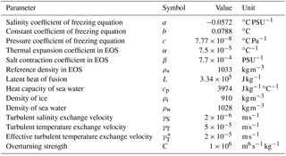
The coefficients in the equation of state (EOS), the turbulent exchange velocities for heat and salt, are taken from Olbers and Hellmer (2010). We linearized the potential freezing temperature equation with a least-squares fit with salinity values over a range of 20–40 PSU and pressure values of 0–107 Pa using Gibbs SeaWater Oceanographic Package of TEOS-10 (McDougall and Barker, 2011). All values are kept constant, except for and C, which vary between experiments. The values of these two parameters are the best-fit from Sect. 3.1.
As PICO is implemented in an ice sheet model with characteristic time scales much slower than typical response times of the ocean, we assume steady state ocean conditions and hence reduce the complexity of the governing equations of the OH10 model. Using this assumption facilitates adaptive box adjustment to grounding line migration, especially since PICO transfers the box model approach into two horizontal dimensions. We assume stable vertical stratification; OH10 found that a circulation state for an unstable vertical water column, which would imply a high (parametrized) diffusive transport between boxes, only occurs transiently (Olbers and Hellmer, 2010). This motivates neglecting the diffusive heat and salt transport between boxes which is small under these conditions. Without diffusive transport between the boxes, some of the original ocean boxes from OH10 become passive and can be incorporated into the governing equations of the set of boxes used in PICO. We explicitly model a single open ocean box which provides the boundary conditions for the boxes adjacent to the ice-shelf base following the overturning circulation, as shown in Fig. 1. In order to better resolve the complex melt patterns, PICO adapts the number of boxes based on the evolving geometry of the ice shelf. These simplifying assumptions allow us to analytically solve the system of governing equations, which is presented in the following two sections. A detailed derivation of the analytic solutions is given in Appendix A. In Sect. 2.3, we describe how the ice-model grid relates to the ocean box geometry of PICO. The system of equations is solved locally on the ice-model grid, as described in Sect. 2.4. Table 1 summarizes the model parameters and typical values.
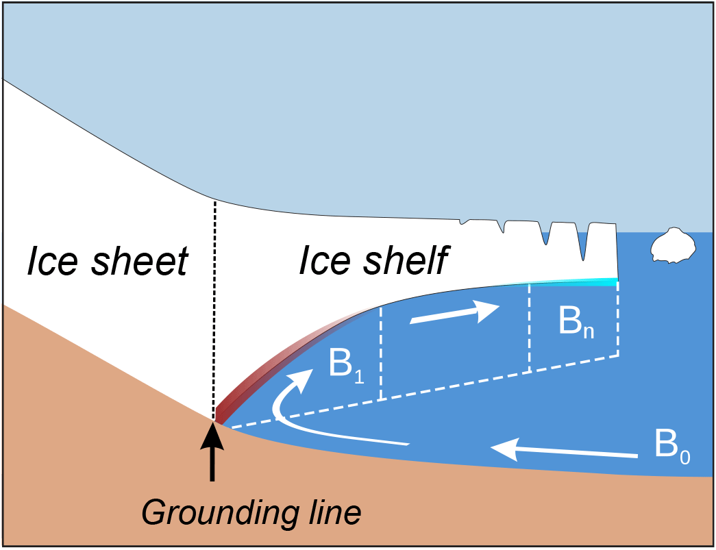
Figure 1Schematic view of the PICO model. The model mimics the overturning circulation in ice-shelf cavities: ocean water from box B0 enters the ice-shelf cavity at the depth of the sea floor and is advected to the grounding line box B1. Freshwater influx from melting at the ice-shelf base makes the water buoyant, causing it to rise. The cavity is divided into n boxes along the ice-shelf base. Generally, the highest melt rates can be found near the grounding line, with lower melt rates or refreezing towards the calving front.
2.1 Physics of the overturning circulation in ice-shelf cavities
PICO solves for the transport of heat and salt between the ocean boxes as depicted in Fig. 1. Although box B0, which is located at depth between the ice-shelf front and the edge of the continental shelf, does not extend into the shelf cavity, its properties are transported unchanged from box B0 to box B1 near the grounding line. The heat and salt balances for all boxes in contact with the ice-shelf base (boxes Bk for ) can be written as
The local application of these equations for each ice model cell is described in Sect. 2.4. Since we assume steady circulation, the terms on the left-hand side are neglected. For the box Bk with volume Vk, heat or salt content change due to advection from the adjacent box Bk−1 with overturning flux q (first term on the right-hand side) and due to advection to the neighboring box Bk+1 (or the open ocean for k=n; second term). Vertical melt flux into the box Bk across the ice–ocean interface with area Ak (third term) and out of the box (fourth term) play a minor role and are neglected in the analytic solution of the equation system employed in PICO (a detailed discussion of these terms is given in Jenkins et al., 2001). The melt rate mk is negative if ambient water freezes to the shelf base. The last term represents heat and salt changes via turbulent, vertical diffusion across the boundary layer beneath the ice–ocean interface. The parameters γT and γS are the turbulent heat and salt exchange velocities which we assume, following OH10, to be constant.
The overturning flux q > 0 is assumed to be driven by the density difference between the ocean reservoir box B0 and the grounding line box B1. This is parametrized as in OH10 as
where C is a constant overturning coefficient that captures effects of friction, rotation and bottom form stress.2 The circulation strength in PICO is hence determined by density changes through sub-shelf melting in the grounding zone box B1. From there, water follows the ice-shelf base towards the open ocean assuming the overturning flux q to be the same for all subsequent boxes. Ocean water densities are computed assuming a linear approximation of the equation of state:
where ∘C, PSU and α, β and ρ* are constants with values given in Table 1.
2.2 Melting physics
Melting physics are derived from the widely used 3-equation model (Hellmer and Olbers, 1989; Holland and Jenkins, 1999), which assumes the presence of a boundary layer below the ice–ocean interface. The temperature at this interface in box Bk is assumed to be at the in situ freezing point Tbk, which is linearly approximated by
where pk is the overburden pressure, here calculated as static-fluid pressure given by the weight of the ice on top. At the ice–ocean interface, the heat flux from the ambient ocean across the boundary layer due to turbulent mixing, , equals the heat flux due to melting or freezing . Neglecting heat flux into the ice, the heat balance equation thus reads
where , ∘C. We obtain the salt flux boundary condition as the balance between turbulent salt transfer across the boundary layer, , and reduced salinity due to melt water input, ,
To compute melt rates, we apply a simplified version of the 3-equations model (Holland and Jenkins, 1999; McPhee, 1992, 1999) which allows for a simple, analytic solution of the system of governing equations. It has been shown that this formulation yields realistic heat fluxes (McPhee, 1992, 1999). This simplification is used only for melt rates, we nevertheless solve for the boundary layer salinity which is central to the solution of the system of equations as detailed in Appendix A. Melt rates are given by
with ambient ocean temperature Tk and salinity Sk in box Bk. Here, we use the effective turbulent heat exchange coefficient . The relation between γT and is discussed in the Appendix A.
2.3 PICO ocean box geometry
PICO is implemented as a module in the three-dimensional ice sheet model PISM as described in Sect. 2.4. Since the original system of box-model equations is formulated for only one horizontal and one vertical dimension, it needed to be extended for the use in the three-dimensional ice sheet model. The system of governing equations as described in the previous two sections is solved for each ice shelf independently. PICO adapts the ocean boxes to the evolving ice shelves at every time step.
For any shelf D, we determine the number of ocean boxes nD by interpolating between 1 and nmax depending on its size and geometry such that larger ice shelves are resolved with more boxes. The maximum number of boxes nmax is a model parameter; a value of 5 is suitable for the Antarctic setup, as discussed further in Sect. 3.2. We determine the number of boxes nD for each individual ice shelf D with
where rd( ) rounds to the nearest integer. Here, dGL(x,y) is the local distance to the grounding line from an ice-model grid cell with horizontal coordinates (x, y), dGL(D) is the maximum distance within ice shelf D and dmax is the maximum distance to the grounding line within the entire computational domain.
Knowing the maximum number of boxes nD for an ice shelf D, we next define the ocean boxes underneath it. The extent of boxes is determined using the distance to the grounding line and the shelf front. The non-dimensional relative distance to the grounding line r is defined as
with dIF(x,y) the horizontal distance to the ice front. We assign all ice cells with horizontal coordinates to box Bk if the following condition is met:
This leads to comparable areas for the different boxes within a shelf, which is motivated in Appendix B. Thus, for example, the box B1 adjacent to the grounding line interacts with all ice shelf grid cells with . Figure 3 shows an example of the ocean box areas for Antarctica. PICO does currently not account for melting along vertical ice cliffs, as, for example, the termini of some Greenland outlet fjords.
2.4 Implementation in the Parallel Ice Sheet Model
PICO is implemented in the open-source Parallel Ice Sheet Model (Bueler and Brown, 2009; Winkelmann et al., 2011). In the three-dimensional, thermo-mechanically coupled, finite-difference model, ice velocities are computed through a superposition of the shallow approximations for the slow, shear-dominated flow in ice sheets (Hutter, 1983) and the fast, membrane-like flow in ice streams and ice shelves (Morland, 1987). In PISM, the grounding lines (diagnosed via the flotation criterion) and ice fronts evolve freely. Grounding line movement has been evaluated in the model intercomparison project MISMIP3d (Feldmann et al., 2014; Pattyn et al., 2013).
PICO is synchronously coupled to the ice-sheet model, i.e., they use the same adaptive time steps. The cavity model provides sub-shelf melt rates and temperatures at the ice–ocean boundary to PISM, with temperatures being at the in situ freezing point. PISM supplies the evolving ice-shelf geometry to PICO, which in turn adjusts in each time step the ocean box geometry to the ice-shelf geometry as described in Sect. 2.3.
PICO computes the melt rates progressively over the ocean boxes, independently for each ice shelf. Since the ice-sheet model has a much higher resolution, each ocean box interacts with a number of ice-shelf grid cells. PICO applies the analytic solutions of the system of governing equations summarized in Sect. 2.1 and 2.2 locally to the ice model grid as detailed below. Model parameters that are varied between the experiments are the effective turbulent heat exchange velocity from the melt parametrization described in Sect. 2.2 and the overturning coefficient C described in Sect. 2.1. The two parameter values are applied to the entire ice sheet.
Input for PICO in the ocean reservoir box B0 is data from observations or large-scale ocean models in front of the ice shelves. Temperature T0 and salinity S0 are averaged at the depth of the bathymetry in the continental shelf region. In box B1 adjacent to the grounding line, PICO solves the system of governing equations in each ice grid cell (x, y) to attain the overturning flux q(x,y), temperature T1(x,y), salinity S1(x,y), and the melting m1(x,y) at its ice–ocean interface (given by the local solution of Eqs. 3, A12, A8 and 8, respectively). The model proceeds progressively from box Bk to box Bk+1 to solve for sub-shelf melt rate , ambient ocean temperature , and salinity (given by the local solution of Eqs. 13, A13 and A8, respectively) based on the previous solutions Sk and Tk in box Bk and conditions at the ice–ocean interface. PICO provides the boundary conditions Tk and Sk to box Bk+1 as the average over the ice-grid cells within box Bk, i.e.,
and analogously for Sk, where 〈 〉 denotes the average.
The overturning is solved in Box B1 and given by . Melt rates in box Bk are computed using the local overburden pressure pk(x,y) in each ice-shelf grid cell that is given by the weight of the ice column provided by PISM, i.e.,
This reflects the pressure dependence of heat available for melting and leads to a depth-dependent melt rate pattern within each box. The implications for energy and mass conservation are discussed in Sects. 3.2 and 4.
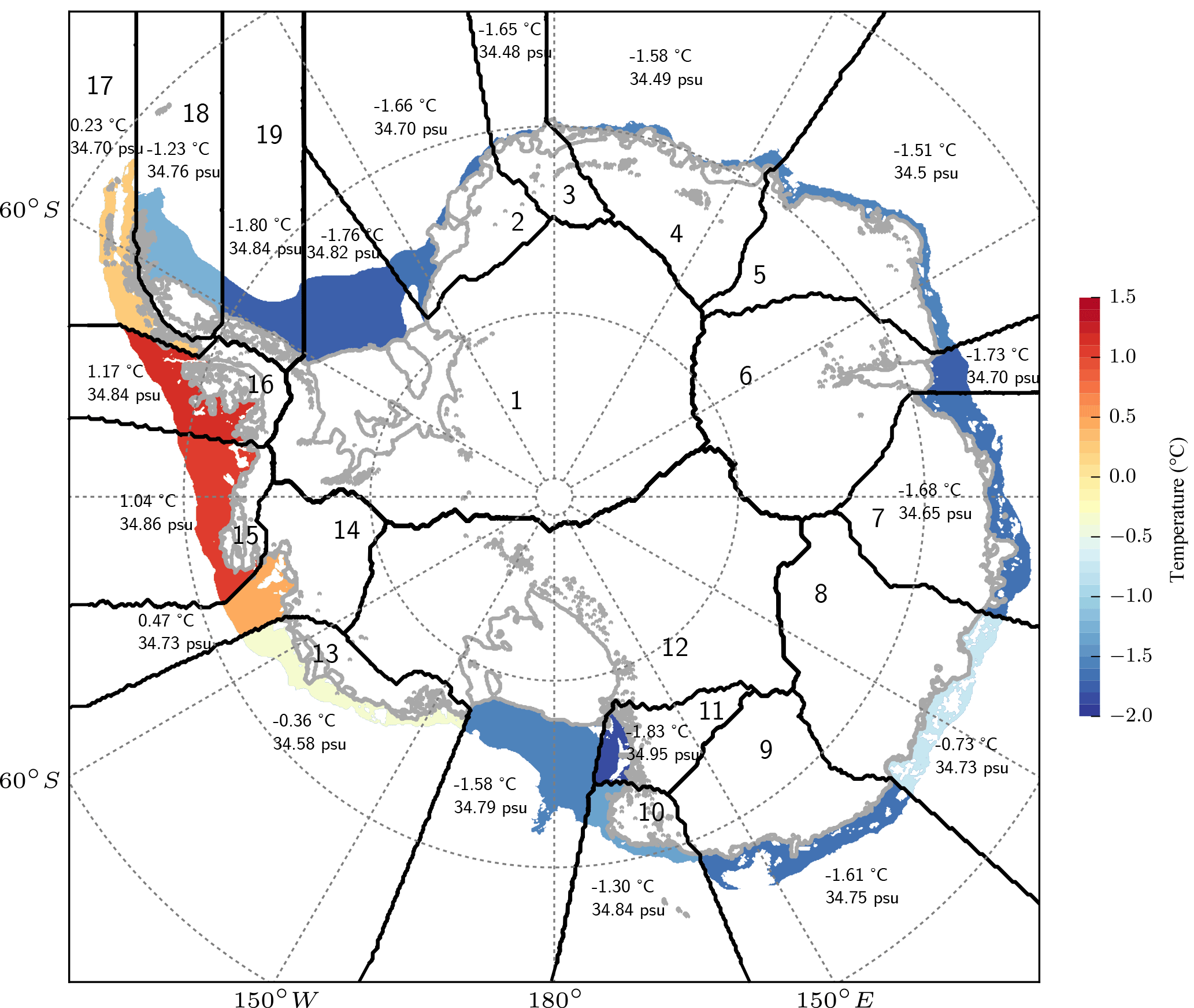
Figure 2PICO input for Antarctic basins. The ice sheet, ice shelves and the surrounding Southern Ocean are split into 19 basins that are based on Zwally et al. (2012) and indicated by black contour lines and labels. For each ice shelf, the governing equations are solved separately with the respective oceanic boundary conditions. For ice shelves that cross basin boundaries, the input is averaged, weighted with the fractional area of the shelf within the corresponding basin. Numbers show the temperature and salinity input in each basin, obtained by averaging observed properties of the ocean water in front of the ice-shelf cavities at depth of the continental shelf (Schmidtko et al., 2014), indicated by the color shading. Grey lines show Antarctic grounding lines and ice-shelf fronts (Fretwell et al., 2013).
We apply PICO to compute sub-shelf melt rates for all Antarctic ice shelves under present-day conditions. Oceanic input for each ice shelf is given by observations of temperature (converted to potential temperature) and salinity (converted to practical salinity) of the water masses occupying the sea floor on the continental shelf (Schmidtko et al., 2014), averaged over the time period 1975 to 2012. Water masses within an ice-shelf cavity originate from source regions: neglecting ocean dynamics, we approximate these by averaging ocean properties on the depth of the continental shelf within regions that are chosen to encompass areas of similar, large-scale ocean conditions. Oceanic input is given for 19 basins of the Antarctic Ice Sheet, which are based on Zwally et al. (2012) and extended to the attached ice shelves and the surrounding Southern Ocean (Fig. 2). For each ice shelf, temperature T0 and salinity S0 in box B0 are obtained by averaging the basin input weighted with the fractional area of the shelf within the corresponding basin. Figure 2 shows the basin-mean ocean temperature (shadings and numbers) and salinity (numbers) used.3
Here, we use from which PICO determines the number of ocean boxes in each shelf via Eq. (9). Figure 3 displays the resulting extent of the ocean boxes for Antarctica, ordered in elongated bands beneath the ice shelves. For the large ice-shelf cavities of Filchner-Ronne and Ross, the ice–ocean boundary is divided into five ocean boxes while smaller ice shelves have two to four boxes (see Table 2). Introducing more than five ocean boxes has a negligible effect on the melt rates, as discussed in Sect. 3.2.
To validate our model, we run diagnostic simulations with PISM+PICO based on bed topography and ice thickness from BEDMAP2 (Fretwell et al., 2013), mapped to a grid with 5 km horizontal resolution. Diagnostic simulations allow us to assess the sensitivity of the model to the parameters C and and to the number of boxes nmax as well as the ice model resolution. Transient behavior is exemplified in a simulation starting from an equilibrium state of the Antarctic Ice Sheet forced with ocean temperature changes, see Video S1 in the Supplement and Sect. 3.3.

Figure 3Extent of PICO ocean boxes for Antarctic ice shelves. Most ice shelves are split into two, three, or four ocean boxes interacting with the ice cells on a much higher resolution. The largest ice shelves, Filchner-Ronne and Ross, have five ocean boxes. One ocean box typically corresponds to many ice-shelf grid cells.
Table 2Results from the reference simulation as displayed in Fig. 5.
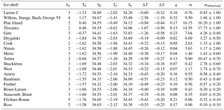
The number of boxes for each is ice-shelf is given by bn, T0 (S0) is the temperature (salinity) in ocean box B0, Tn (Sn) the temperature (salinity) averaged over the ocean box at the ice-shelf front, and . m is the average sub-shelf melt rate, mobserved the observed melt rates from Rignot et al. (2013). q is the overturning flux. Unit of temperatures is ∘C, salinity is given in PSU, melt rates in m a−1 and overturning flux in Sv.
3.1 Sensitivity to model parameters C and
We test the sensitivity of sub-shelf melt rates to the model parameters for overturning strength Sv m3 kg−1 and the effective turbulent heat exchange velocity m s−1. These ranges encompass the values identified in OH10, discussed further in Appendix A. The same parameters for C and are applied to all shelves. We constrain the results by the following qualitative criteria (1) and (2), as well as the quantitative constraints (3) and (4), summarized in Fig. 4:
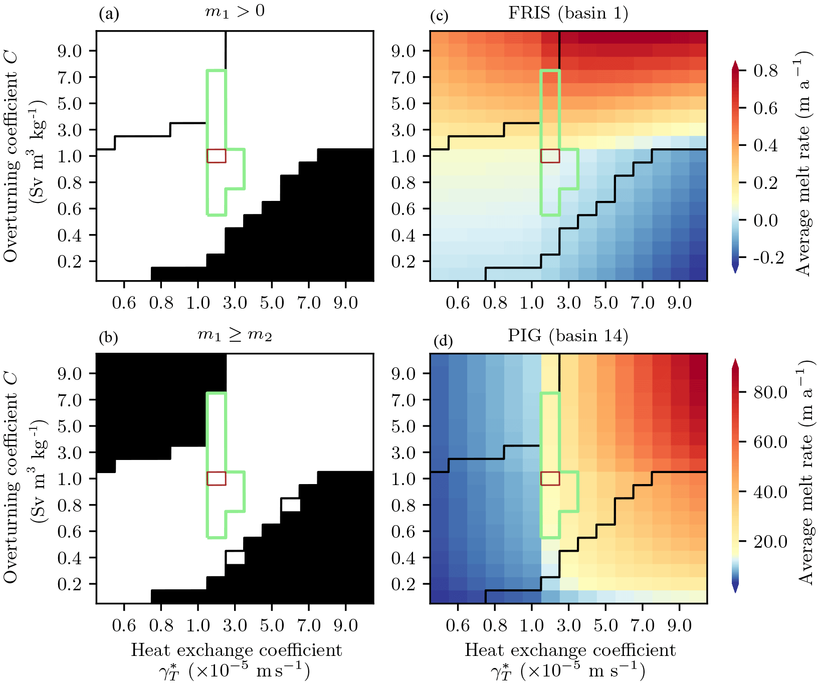
Figure 4Sensitivity of PICO sub-shelf melt rates to the overturning coefficient C and the effective turbulent heat exchange coefficient . Black contour indicates the valid range of parameters, all other parameter combinations are excluded by one of the following criteria: no freezing may occur in the first ocean box (a), mean basal melt rates must decrease between the first and second ocean box (b). Green contour indicates the valid range of parameters where the following quantitative constraints are additionally met: mean basal melt rates for Filchner-Ronne Ice Shelf should be within the range of 0.01 to 1.0 m a−1 (c), mean basal melt rates for Pine Island Glacier Ice Shelf should be within the range of 10.0 to 25.0 m a−1 (d). The best-fit parameters (brown contour) minimize the root-mean-square error of mean melt rates to observations for both ice shelves.
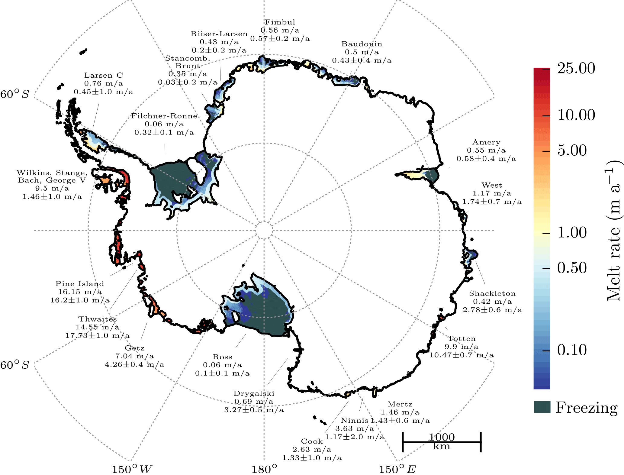
Figure 5Sub-shelf melt rates for present-day Antarctica computed with PISM+PICO. The mean melt rate per ice shelf (upper numbers) is compared to the observed melt rates (lower numbers with uncertainty ranges) from Rignot et al. (2013). In the model, the same parameters m s−1 and C=1 Sv m3 kg−1 are applied to all ice shelves around Antarctica. The respective oceanic boundary condition are shown in Fig. 2. Ice geometry and bedrock topography are from the BEDMAP2 data set on 5 km resolution (Fretwell et al., 2013). Refreezing occurs in some parts of the larger shelves like Filchner-Ronne and Ross.
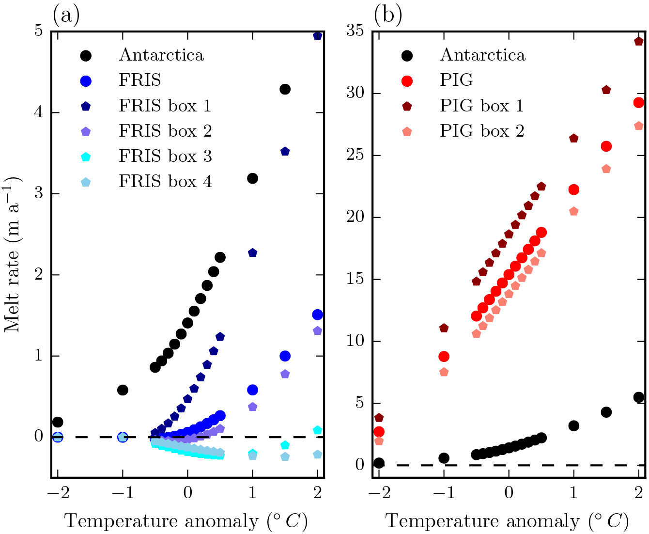
Figure 6Sensitivity of PICO sub-shelf melt rates to ocean temperature changes for the entirety of Antarctica (black), Filchner-Ronne Ice Shelf (blue), and Pine Island Glacier Ice Shelf (red). Ocean input temperatures are varied by 0.1 up to 2 ∘C. Melting depends quadratically on temperature for “cold” cavities like the one adjacent to Filchner-Ronne, and linearly for “warm” cavities like the ones in the Amundsen Region.
Criterion (1). Freezing must not occur in the first box B1 of any ice shelf, i.e., the ocean box closest to the grounding line. Freezing in box B1 would increase ambient salinity, and since the overturning circulation in ice-shelf cavities is mainly haline driven, the circulation would shut down, violating the model assumption q>0 (see Sect. 2). As shown in Fig. 4a, the condition is not met for a combination of relatively high turbulent heat exchange and relatively low overturning parameters. In such cases, freezing near the grounding line occurs because of the strong heat exchange between the ambient ocean and the ice–ocean boundary in box B1 that cannot be balanced by the resupply of heat from the open ocean through overturning.
Criterion (2). Sub-shelf melt rates must decrease between the first and second box for each ice shelf. This condition is based on general observations of melt-rate patterns and on the assumption that ocean water masses move consecutively through the boxes and cool down along the way, as long as melting in these boxes outweighs freezing. As shown in Fig. 4b, this condition is violated for either high overturning and low turbulent heat exchange or, vice versa, low overturning and high turbulent heat exchange. An appropriate balance between the strength of these values is hence necessary for a realistic melt rate pattern.
If criterion (1) or (2) fails, basic assumptions of PICO are violated. Thus, we choose the model parameters and C such that both criteria are strictly met. The following quantitative, observational constraints (3) and (4) compare modeled average melt rates with observations and thus depend on our choice of valid ranges. We choose Filchner-Ronne Ice Shelf and the ice shelf adjacent to Pine Island Glacier to further constrain our model parameters for Antarctica. These shelves represent two different types regarding both the mode of melting and the ice-shelf size.
Observational constraint (3). Average melt rates in Filchner-Ronne Ice Shelf comply with the classification of a “cold” cavity and lie between 0.01 and 1.0 m a−1 (Fig. 4c).
Observational constraint (4). For Pine Island Glacier, with “warm” ocean conditions, average melt rates lie between 10 and 25 m a−1 (Fig. 4d).
Generally, an increase in overturning strength C will supply more heat and thus yield higher melt rates, especially for the large and “cold” ice shelves like Filchner-Ronne. Larger C leads to higher melt rates also in the smaller and “warm” Pine-Island Glacier Ice Shelf but the effect is less pronounced. In contrast, the turbulent heat exchange alters melting, particularly in small ice shelves, while it might decrease melt rates in large ice shelves with “cold” cavities. Hence, modeled melting in the Filchner-Ronne Ice Shelf is dominated by overturning while in the Amundsen region melting is dominated by turbulent exchange across the ice–ocean boundary layer. For three different parameter combinations, the resulting spatial patterns of melt rates in the Filchner-Ronne and Pine Island regions are displayed in Fig. S1 in the Supplement.
All of the above criteria restrict the parameter space to a bounded set with lower and upper limits as depicted by the green contour lines in Fig. 4. We determine a best-fit pair of parameters which minimizes the root-mean-square error of average melt rates for both ice shelves. The valid range of model parameters around the best-fit parameters with C=1 Sv m3 kg−1 and m a−1 compares well with parameters found in OH10 and Holland and Jenkins (1999), discussed further in Appendix A.
3.2 Diagnostic melt rates for present-day Antarctica
Using the best-fit values C=1 Sv m3 kg−1 and m s−1 found in Sect. 3.1, we apply PICO to present-day Antarctica, solving for sub-shelf melt rates and water properties in the ocean boxes. This model simulation is referred to as “reference simulation” hereafter.
The average melt rates computed with PICO range from 0.06 m a−1 under the Ross Ice Shelf to 16.15 m a−1 for the Amundsen Region (Fig. 5). Consistent with the model assumptions, melt rates are highest in the vicinity of the grounding line and decrease towards the calving front. In some regions of the large ice shelves, refreezing occurs, e.g., towards the center of Filchner-Ronne or Amery ice shelves. The melt pattern depends on the local pressure melting temperature. Thus, melt rates are highest where the shelf is thickest, i.e., near the grounding lines within box B1. Furthermore, freezing and melting can occur in the same box determined by local ice-shelf thickness. For the vast majority of ice shelves, the modeled average melt rates compare well with the observed ranges derived from Table 1 in Rignot et al. (2013). Exceptions are the Wilkins and Stange ice shelves (in basin 16) with average modeled melt rates of 9.50 m a−1, which is much higher than the observed range of 1.46 ± 1.0 m a−1. This is most likely due to the ocean temperature input for this basin (1.17 ∘C, see Fig. 2) which is higher than for the basin containing Pine Island located nearby (0.47 ∘C, basin 14), explaining why the melt rates are of the same order of magnitude in these basins. Modification of water masses flowing into the shelf cavities, not captured by PICO, might explain the low observed melt rates in this area despite the relatively high ocean temperatures.
For all ice shelves, ocean temperatures and salinities consistently decrease in overturning direction, i.e., from the ocean reservoir box B0 to the last box adjacent to the ice front Bn, as shown in Table 2. Most shelves contain small areas with accretion with a maximum rate of −1.22 m a−1 for the Amery Ice Shelf, see Table S1 in the Supplement. No freezing occurs at the Western Antarctic Peninsula nor in the Amundsen and Bellingshausen Seas. A detailed map of sub-shelf melt rates in this region as well as for Filchner-Ronne Ice Shelf can be found in the middle panels of Fig. S1. For the Filchner-Ronne Ice Shelf melt rates vary between −0.67 and 1.76 m a−1 and for Pine Island Glacier, melt rates range from 12.39 to 21.01 m a−1.
PICO tends to smooth out melt rate patterns, see Fig. S4: for Filchner-Ronne and Ross ice shelves the deviations in observed melt rates (Moholdt et al., 2016) from the average melting are larger than the deviations modeled in PICO. The box-wide averages compare well and are at the same order of magnitude for both ice shelves, except for modeled accretion in the later boxes towards the shelf front which is not reflected in the observations. This disagreement might be explained by the fact that the overturning circulation in the model cannot reach neutral density and detach from the ice-shelf base while flowing towards the shelf front.
Aggregated over all Antarctic ice shelves, the total melt flux is 1718 Gt a−1, close to the observed estimate of 1500 ± 237 Gt a−1 (Rignot et al., 2013). Overturning fluxes in our reference simulation range from 0.02 Sv for the small Drygalski Ice Shelf to 0.32 Sv for Wilkings, Stange, Bach and George VI ice shelves. Because these are treated in PICO as one ice shelf and they have a high input temperature, these ice shelves reach together this high overturning value. The second highest value of 0.23 Sv is found for Getz Ice Shelf in the Bellingshausen Sea. These overturning fluxes compare well with the estimates in OH10.
PICO solves the system of governing equations locally in each ice-model grid cell and calculates input for each ocean box as an average over the previous box as described in Sect. 2.4. Due to these model assumptions and because temperature, salinity, overturning and melting are non-linear functions of pressure in the first box (Eq. A12), mass and energy are a priori not perfectly conserved. In Table S1, we compare (within individual shelves) heat fluxes into the ice-shelf cavities with the heat flux out of the cavities into the ocean and the latent heat flux for melting. For the whole of Antarctica, the deviation in heat flux is 403.63 G J s−1 which is equivalent to 2.2 % of the latent heat flux for melting. The per basin deviations are generally low (< 5 %), except around the large Filchner-Ronne and Ross ice shelves (68 and 43 %). In PICO we assume q to be constant, neglecting changes due to melt water input along the shelf base. This melt water input amounts to 3.06 % or less of the overturning flux within ice shelves, and 0.62 % for the entire continent, discussed in Sect. 2.1.
Melt rates are strongly affected by changes in the ambient ocean temperatures, see Fig. 6. The dependence is approximately linear for high and quadratic for lower ambient ocean temperatures. This relationship is similar to the one observed in OH10 and as expected from the governing equations. In Pine Island Glacier, melt rates increase by approximately 6 m a−1 per degree of warming. Changes in the ice-sheet model resolution have little effect on the resulting melt rates (Fig. S2). For increasing the maximum number of boxes nmax, average melt rates converge to almost constant values for within all basins, compare Fig. S3.
3.3 Transient evolution of PICO boxes and melt rates
PICO is capable of adjusting to changing ice-shelf geometries and migrating grounding lines. We demonstrate its behavior as a module in PISM in a transient simulation. Based on an Antarctic equilibrium state at 8 km resolution comparable to the state submitted to initMIP (Nowicki et al., 2016), we run PISM+PICO over time with a simple temperature forcing applied: starting from equilibrium conditions, ocean temperatures increase linearly over 50 years until an ocean-wide warming of 1 ∘C is reached. It is then held constant over the next 250 modeled years. The Video S1 shows the temporal evolution of the ocean temperature input for the ice shelf adjacent to Pine Island Glacier as well as the Filchner-Ronne Ice Shelf. The ocean temperature increase enhances the sub-shelf melting for both ice shelves, especially in the first box. Ice-shelf thinning reduces buttressing and causes the grounding lines to retreat with the ocean boxes adjusting accordingly.
PICO models the dominant vertical overturning circulation in ice-shelf cavities and translates ocean conditions in front of the ice shelves, either from observations or large-scale ocean models, into physically based sub-shelf melt rates. For present-day ocean fields and ice-shelf cavity geometries, PICO as an ocean module in PISM reproduces average melt rates of the same order of magnitude as observations for most Antarctic ice shelves. With a single combination of overturning parameter C and effective turbulent heat exchange parameter applied to all shelves, a wide range of melt rates for the different ice shelves is obtained, reproducing the large-scale patterns observed in Antarctica. The results are consistent across different ice-sheet and cavity model resolutions. Additionally, PICO reproduces the common pattern of maximum melt close to the grounding line and decreasing melt rates towards the ice-shelf front, eventually with re-freezing in the shallow parts of the large ice shelves. The governing model equations are solved for individual grid cells of the ice sheet model (and not for each ocean box with representative depth value), which allows spatial variability in the resulting melt rate field at comparatively smaller scale. PICO can adapt to evolving cavities and is applicable to ice shelves in two horizontal dimensions. It is hence suited as a sub-shelf melt module for ice-sheet models.
Yet PICO is a coarse model designed as an ocean coupler for large-scale ice-sheet models. It is based on the OH10 model and hence shares some simplifying assumptions with that model: PICO does not resolve ocean dynamics and it parameterizes the vertical overturning circulation in the ice-shelf cavities which is given by one value for each ice shelf. The underlying box model equations of PICO do not resolve horizontal ocean circulation in the ice-shelf cavities driven by the Coriolis force nor seasonal melt variation due to intrusion of warm water from the calving front during Austral summer. Hence, we do not expect that horizontal variations or small scale patterns of basal melt are accurately captured in PICO. Due to the box model formulation, maximum melting in PICO is found directly at the grounding line and not slightly downstream as seen in the high-resolution coupled ice–ocean simulation by, e.g., De Rydt and Gudmundsson (2016). We find that PICO tends to produce smoother melt rate patterns than observed, though the box-wide averages are in good agreement with observations. The effect on ice dynamics of small-scale differences in melt patterns in relation to the large-scale mean melt fluxes is not well established yet and needs further investigation. Following OH10, meltwater does not contribute to the volume flux in the cavity in PICO, introducing a minor error regarding mass conservation. The relative error regarding mass conservation is however small and below 0.7 % of the total overturning strength in our reference run.
A necessary condition for the box model to work is further the assumption that melting outweighs accretion in box B1 which is consistent with the majority of available observations. In PICO, melt rates show a quadratic dependency on ocean temperature input for lower temperatures, e.g., in the Filchner-Ronne basin, and a rather linear dependency for higher temperatures, e.g., in the Amundsen basin. This is consistent with the results from OH10 and the implemented melting physics assuming a constant coefficient for turbulent heat exchange. In contrast, P. R. Holland et al. (2008) employ a dependency of the turbulent heat exchange coefficient on the velocity of the overturning circulation, suggesting melt rates to respond quadratically to warming of the ambient ocean water. Here we follow the approach taken in OH10.
Differently from the OH10 model and relying on much longer timescales of ice dynamics in comparison to ocean dynamics, PICO assumes the overturning circulation to be in steady state. In their analysis, OH10 find unstable vertical water columns to occur only transiently, and hence for PICO a stable stratification of the vertical water column is assumed. Under these conditions, diffusive transport between the boxes is generally small in OH10 and it is hence omitted in PICO. Because PICO also does not consider vertical variations in ambient ocean density, under-ice flow is prevented from reaching neutral density and detaching from the ice-shelf base on its way towards the shelf front. The spatial pattern of melting closer to the calving front of cold ice shelves may in such cases be not represented well.
PICO input is determined by averaging bottom temperatures and salinities over the continental shelf, this is done for 19 different basins. Hence PICO – as a coarse model – misses the nuances of how ocean currents transport and modify CDW over the regions being averaged. The procedure to determine melt rates in PICO is based on the assumption that ocean water that is present on the continental shelf can access the ice-shelf cavities and reach their grounding lines. This implies for example, that barriers like sills that may prevent intrusion of warm CDW are not accounted for and might explain why PICO melting is too high for the ice shelves located along the Southern Antarctic Peninsula. Such phenomena could be tested by varying the ocean input of PICO by evolving the temperature and salinity outside of the cavity over time. Because of the dependence of sub-shelf melting on the local pressure of the ice column above, the model is not fully energy conserving. For the estimated heat fluxes, the relative error is lower than 2.2 % of the latent heat flux due to sub-shelf melting. Hence, we consider our choice of model simplifications as justified, as it introduces small errors in the heat and mass balances in our reference simulation.
PICO is computationally fast, as it uses analytic solutions of the equations of motion with a small number of boxes along the ice shelf. As boundary conditions for PICO are aggregated based on predefined regional basins, the model can act as an efficient coupler of large-scale ice-sheet and ocean models. For this purpose, heat flux into the ice should be added to the boundary layer melt formulation.
The Antarctic Ice Sheet plays a vital role in modulating global sea level. The ice grounded below sea level in its marine basins is susceptible to ocean forcing and might respond nonlinearly to changes in ocean boundary conditions (Mercer, 1978; Schoof, 2007). We therefore need carefully estimated conditions at the ice–ocean boundary to better constrain the dynamics of the Antarctic ice and its contribution to sea-level rise for the past and the future.
The PICO model presented here provides a physics-based yet efficient approach for estimating the ocean circulation below ice shelves and the heat provided for ice-shelf melt. The model extends the one-horizontal dimensional ocean box model by OH10 to realistic ice-shelf geometries following the shape of the grounding line and calving front. PICO is a comparably simple alternative to full ocean models, but goes beyond local melt parameterizations, which do not account for the circulation below ice shelves. We find a set of possible parameters for present-day ocean conditions and ice geometries which yield PICO melt rates in agreement with average melt rate observations. PICO qualitatively reproduces the general pattern of ice-shelf melt, with high melting at the grounding line and low melting or refreezing towards the calving front. Its sensitivity to changes in input ocean temperatures and model parameters is comparable to earlier estimates (Holland and Jenkins, 1999; Olbers and Hellmer, 2010). The model accurately captures the large variety of observed Antarctic melt rates using only two calibrated parameters applied to all ice shelves.
The ocean models that are part of the large Earth system and global circulation models do not yet resolve the circulation below ice shelves. PICO is able to fill this gap and can be used as an intermediary between global circulation models and ice sheet models. We expect that PICO will be useful for providing ocean forcing to ice sheet models with the standardized input from climate model intercomparison projects like CMIP5 and CMIP6 (Eyring et al., 2016; Meehl et al., 2014; Taylor et al., 2012). Since PICO can deal with evolving ice-shelf geometries in a computationally efficient way, it is in particular suitable for modeling the ice sheet evolution on paleo-climate timescales as well as for future projections.
PICO is implemented as a module in the open-source Parallel Ice Sheet Model (PISM). The source code is fully accessible and documented as we want to encourage improvements and implementation in other ice sheet models. This includes the adaption to other ice sheets than present-day Antarctica.
The PICO code used for this publication is available under Reese et al. (2018). For further use of PICO please refer to the latest version at https://github.com/pism/pism/commits/dev.
The data that support the findings of this study are available from the corresponding authors upon request.
Here, we derive the analytic solutions of the equations system describing the overturning circulation (see Sect. 2.1) and the melting at the ice–ocean interface (see Sect. 2.2).
For box Bk with k>1 we solve progressively for melt rate mk, temperature Tk and salinity Sk in box Bk, dependent on the local pressure pk, the area of box adjacent to the ice-shelf base Ak and the temperature Tk−1 and salinity Sk−1 of the upstream box Bk−1. For box B1, we additionally solve for the overturning q as explained below. These derivations advance the ideas presented in the appendix of OH10. Assuming steady state conditions, the balance Eqs. (1) and (2) for box Bk from Sect. 2.1 are
The heat fluxes balance at the boundary layer interface, i.e., the heat flux across the boundary layer due to turbulent mixing equals the heat flux due to melting or freezing , omitting the heat flux into the ice. This yields
where , ∘C. Regarding the salt flux balance in the boundary layer, with at the lower interface of the boundary layer and “virtual” salt flux due to meltwater input , we obtain
Inserting Eqs. (A2) and (A3) into Eqs. (A1) yields
Comparing ∘C, allows us to neglect the last term in the temperature equation. Considering the last two terms of the salinity equation, we find that , allowing us to neglect the terms containing Sbk, which simplifies the equations to
We use a simplified version of the melt law described by McPhee (1992) and detailed in Sect. 2.2, which makes use of Eqs. (6) and (5) in which the salinity in the boundary layer Sbk is replaced by salinity of the ambient ocean water:
Holland and Jenkins (1999) suggest that this simplification requires to be a factor of 1.35 to 1.6 smaller than γT in the 3-equation formulation for the constant values of γT ranging from to m s−1 used in OH10. This implies that ranges from to m s−1, which is consistent with the parameter range we derive in Sect. 3.1. We apply this assumption in the computation of melt rates. For the solution of the transport Eqs. (A1), it is essential to take the salinity of the boundary layer Sbk into account, since otherwise the salinity transport equation would reduce to and the overturning circulation, which is predominantly haline driven, would be reduced. Inserting the simplified melt law in Eq. (A4) yields
Replacing , , , and , we obtain
We simplify the previous equations as follows. Rewriting Eq. (A6) as
and inserting it into Eq. (A7), we obtain
Note that we can divide the first line by q since, by the model assumptions, q>0. Because ∘C, we may approximate
Using this approximation, we may proceed to solve the system of equations. Since we also need to solve for the overturning q in box B1, which is adjacent to the grounding line, a slightly different approach is needed than for the other boxes, as discussed in the next section.
Solution for box B1
The overturning flux q is parameterized as
in the model, see Sect. 2.1. Substituting this equation into Eqs. (A6) and (A7), we obtain
Inserting the approximation for y from Eq. (A8) into the Eq. (A10), we obtain a quadratic equation for x,
with . Since , we can omit the last part of the last term,
Rearranging (assuming that , which we demonstrate below), we obtain
and hence we obtain the solution
The temperature in the box B1 near the grounding line is supposed to be smaller than in the ocean box B0, since, in general, melting will occur in box B1 and hence T1<T0, or equivalently . Furthermore, we know that is positive, as all factors are positive. Since , and , it follows that βs>α. This means that the first summand of Eq. (A12) is negative and the second (negative) solution can be excluded. From here, we use and to solve for T1, S1, m1 and q.
Solution for box Bk, k>1
Now, we give the solution for the other boxes Bk with k>1. By inserting the approximation for y in Eq. (A8) into Eq. (A6), we can solve for x as
The denominator is positive, as all terms are positive, and the sign of the numerator depends on T*. The equation can now be solved for Tk, and then Eq. (A8) for Sk and Eq. (13) for mk.
Here, we want to motivate the rule that determines the extent of the boxes under each ice shelf. The rule aims at equal areas for all boxes. Assuming a half-circle with radius r=1, we want to split it into a fixed number n of equal-area rings. Generalized to the individual shapes of ice shelves, we will define the “radius” of an ice shelf as . We define r1=1 the outer (grounding-line ward) radius of the half-circle ring covering an area A1 and corresponding to box B1 adjacent to the grounding line, r2 as the outer radius of second outer-most half-ring, etc. The box Bk is then given by all shelf cells with horizontal coordinates (x, y) such that where is the center point of the circle. We can use these to determine the areas . If we require that , then, solving progressively, . By our assumption is r1=1, hence . This implies that and thus . Hence, the box Bk for is defined as .
The supplement related to this article is available online at: https://doi.org/10.5194/tc-12-1969-2018-supplement.
All authors designed the model. RW conceived the study. RR, RW, TA, and MM implemented PICO as a module in PISM. RR conducted the model experiments. MM created the Antarctic equilibrium simulation for the Video S1 in the Supplement. RR prepared the manuscript with contributions from all co-authors.
The authors declare that they have no conflict of interest.
Development of PISM is supported by NASA grant NNX17AG65G and NSF grants PLR-1603799 and PLR-1644277. Torsten Albrecht was supported by DFG priority program SPP 1158, project numbers LE1448/6-1 and LE1448/7-1. Matthias Mengel was supported by the AXA Research Fund. Ronja Reese was supported by the German Academic National Foundation, the postgraduate scholarship programme of the state of Brandenburg and the Evangelisches Studienwerk Villigst. The project is further supported by the German Climate Modeling Initiative (PalMod) and the Leibniz project DominoES. Xylar Asay-Davis was supported by the US Department of Energy, Office of Science, Office of Biological and Environmental Research under award no. DE-SC0013038. The authors gratefully acknowledge the European Regional Development Fund (ERDF), the German Federal Ministry of Education and Research and the Land Brandenburg for supporting this project by providing resources on the high performance computer system at the Potsdam Institute for Climate Impact Research.
We thank Frank Pattyn and the anonymous reviewer for their helpful comments
on the manuscript. We are grateful to Constantine Khroulev for his excellent
support in improving the implementation of PICO in PISM. We are very thankful
to Hartmut H. Hellmer and Dirk Olbers for their helpful comments and their
ongoing support in further developing their original ocean box
model.
Edited by: Eric Larour
Reviewed by: Frank Pattyn and one anonymous referee
Asay-Davis, X. S., Cornford, S. L., Durand, G., Galton-Fenzi, B. K., Gladstone, R. M., Gudmundsson, G. H., Hattermann, T., Holland, D. M., Holland, D., Holland, P. R., Martin, D. F., Mathiot, P., Pattyn, F., and Seroussi, H.: Experimental design for three interrelated marine ice sheet and ocean model intercomparison projects: MISMIP v. 3 (MISMIP +), ISOMIP v. 2 (ISOMIP +) and MISOMIP v. 1 (MISOMIP1), Geosci. Model Dev., 9, 2471–2497, https://doi.org/10.5194/gmd-9-2471-2016, 2016. a
Beckmann, A. and Goosse, H.: A parameterization of ice shelf-ocean interaction for climate models, Ocean Model., 5, 157–170, https://doi.org/10.1016/S1463-5003(02)00019-7, 2003. a
Beckmann, J., Perrette, M., and Ganopolski, A.: Simple models for the simulation of submarine melt for a Greenland glacial system model, The Cryosphere, 12, 301–323, https://doi.org/10.5194/tc-12-301-2018, 2018. a
Bueler, E. and Brown, J.: Shallow shelf approximation as a “sliding law” in a thermomechanically coupled ice sheet model, J. Geophys. Res., 114, F03008, https://doi.org/10.1029/2008JF001179, 2009. a, b
Carroll, D., Sutherland, D. A., Shroyer, E. L., Nash, J. D., Catania, G. A., and Stearns, L. A.: Modeling Turbulent Subglacial Meltwater Plumes: Implications for Fjord-Scale Buoyancy-Driven Circulation, J. Phys. Oceanogr., 45, 2169–2185, https://doi.org/10.1175/JPO-D-15-0033.1, 2015. a
Depoorter, M. A., Bamber, J. L., Griggs, J. A., Lenaerts, J. T. M., Ligtenberg, S. R. M., van den Broeke, M. R., and Moholdt, G.: Calving fluxes and basal melt rates of Antarctic ice shelves., Nature, 502, 89–92, https://doi.org/10.1038/nature12567, 2013. a
De Rydt, J. and Gudmundsson, G. H.: Coupled ice shelf-ocean modeling and complex grounding line retreat from a seabed ridge, J. Geophys. Res.-Earth, 121, 865–880, https://doi.org/10.1002/2015JF003791, 2016. a, b
Dupont, T. K. and Alley, R. B.: Assessment of the importance of ice-shelf buttressing to ice-sheet flow, Geophys. Res. Lett., 32, L04503, https://doi.org/10.1029/2004GL022024, 2005. a
Eyring, V., Bony, S., Meehl, G. A., Senior, C. A., Stevens, B., Stouffer, R. J., and Taylor, K. E.: Overview of the Coupled Model Intercomparison Project Phase 6 (CMIP6) experimental design and organization, Geosci. Model Dev., 9, 1937–1958, https://doi.org/10.5194/gmd-9-1937-2016, 2016. a
Favier, L., Durand, G., Cornford, S. L., Gudmundsson, G. H., Gagliardini, O., Gillet-Chaulet, F., Zwinger, T., Payne, A. J., and Le Brocq, A. M.: Retreat of Pine Island Glacier controlled by marine ice-sheet instability, Nat. Clim. Change, 5, 117–121, https://doi.org/10.1038/nclimate2094, 2014. a
Feldmann, J., Albrecht, T., Khroulev, C., Pattyn, F., and Levermann, A.: Resolution-dependent performance of grounding line motion in a shallow model compared with a full-Stokes model according to the MISMIP3d intercomparison, J. Glaciol., 60, 353–360, https://doi.org/10.3189/2014JoG13J093, 2014. a
Fretwell, P., Pritchard, H. D., Vaughan, D. G., Bamber, J. L., Barrand, N. E., Bell, R., Bianchi, C., Bingham, R. G., Blankenship, D. D., Casassa, G., Catania, G., Callens, D., Conway, H., Cook, A. J., Corr, H. F. J., Damaske, D., Damm, V., Ferraccioli, F., Forsberg, R., Fujita, S., Gim, Y., Gogineni, P., Griggs, J. A., Hindmarsh, R. C. A., Holmlund, P., Holt, J. W., Jacobel, R. W., Jenkins, A., Jokat, W., Jordan, T., King, E. C., Kohler, J., Krabill, W., Riger-Kusk, M., Langley, K. A., Leitchenkov, G., Leuschen, C., Luyendyk, B. P., Matsuoka, K., Mouginot, J., Nitsche, F. O., Nogi, Y., Nost, O. A., Popov, S. V., Rignot, E., Rippin, D. M., Rivera, A., Roberts, J., Ross, N., Siegert, M. J., Smith, A. M., Steinhage, D., Studinger, M., Sun, B., Tinto, B. K., Welch, B. C., Wilson, D., Young, D. A., Xiangbin, C., and Zirizzotti, A.: Bedmap2: improved ice bed, surface and thickness datasets for Antarctica, The Cryosphere, 7, 375–393, https://doi.org/10.5194/tc-7-375-2013, 2013. a, b, c
Goldberg, D. N., Little, C. M., Sergienko, O. V., Gnanadesikan, A., Hallberg, R., and Oppenheimer, M.: Investigation of land ice–ocean interaction with a fully coupled ice-ocean model: 1. Model description and behavior, J. Geophys. Res., 117, F02037, https://doi.org/10.1029/2011JF002246, 2012. a
Greenbaum, J. S., Blankenship, D. D., Young, D. A., Richter, T. G., Roberts, J. L., Aitken, A. R. A., Legresy, B., Schroeder, D. M., Warner, R. C., van Ommen, T. D., and Siegert, M. J.: Ocean access to a cavity beneath Totten Glacier in East Antarctica, Nat. Geosci., 8, 294–298,https://doi.org/10.1038/NGEO2388, 2015. a
Gudmundsson, G. H., Krug, J., Durand, G., Favier, L., and Gagliardini, O.: The stability of grounding lines on retrograde slopes, The Cryosphere, 6, 1497–1505, https://doi.org/10.5194/tc-6-1497-2012, 2012. a
Hellmer, H. and Olbers, D.: A two-dimensional model for the thermohaline circulation under an ice shelf, Antarct. Sci., 1, 325–336, https://doi.org/10.1017/S0954102089000490, 1989. a
Hellmer, H. H., Kauker, F., Timmermann, R., and Hattermann, T.: The fate of the southern Weddell Sea continental shelf in a warming climate, J. Climate, 30, 4337–4350, https://doi.org/10.1175/JCLI-D-16-0420.1, 2017. a
Holland, D. M. and Jenkins, A.: Modeling Thermodynamic Ice–Ocean Interactions at the Base of an Ice Shelf, J. Phys. Oceanogr., 29, 1787–1800, https://doi.org/10.1175/1520-0485(1999)029<1787:MTIOIA>2.0.CO;2, 1999. a, b, c, d, e
Holland, D. M., Thomas, R. H., de Young, B., Ribergaard, M. H., and Lyberth, B.: Acceleration of Jakobshavn Isbrætriggered by warm subsurface ocean waters, Nat. Geosci., 1, 659–664, https://doi.org/10.1038/ngeo316, 2008. a
Holland, P. R., Feltham, D. L., and Jenkins, A.: Ice Shelf Water plume flow beneath Filchner-Ronne Ice Shelf, Antarctica, J. Geophys. Res., 112, C05044, https://doi.org/10.1029/2006JC003915, 2007. a
Holland, P. R., Jenkins, A., and Holland, D. M.: The Response of Ice Shelf Basal Melting to Variations in Ocean Temperature, J. Climate, 21, 2558–2572, https://doi.org/10.1175/2007JCLI1909.1, 2008. a
Hutter, K.: Theoretical glaciology: material science of ice and the mechanics of glaciers and ice sheets, Springer, vol. 1, 1983. a
Jacobs, S. S., Hellmer, H., Doake, C. S. M., Jenkins, A., and Frolich, R. M.: Melting of ice shelves and the mass balance of Antarctica, J. Glaciol., 38, 375–387, https://doi.org/10.3189/S0022143000002252, 1992. a
Jacobs, S. S., Jenkins, A., Giulivi, C. F., and Dutrieux, P.: Stronger ocean circulation and increased melting under Pine Island Glacier ice shelf, Nat. Geosci., 4, 519–523, https://doi.org/10.1038/ngeo1188, 2011. a
Jenkins, A.: A one-dimensional model of ice shelf-ocean interaction, J. Geophys. Res., 96, 20671–20677, https://doi.org/10.1029/91JC01842, 1991. a
Jenkins, A.: Convection-Driven Melting near the Grounding Lines of Ice Shelves and Tidewater Glaciers, J. Phys. Oceanogr., 41, 2279–2294, https://doi.org/10.1175/JPO-D-11-03.1, 2011. a
Jenkins, A., Hellmer, H. H., and Holland, D. M.: The Role of Meltwater Advection in the Formulation of Conservative Boundary Conditions at an Ice-Ocean Interface, J. Phys. Oceanogr., 31, 285–296, https://doi.org/10.1175/1520-0485(2001)031<0285:TROMAI>2.0.CO;2, 2001. a
Joughin, I., Alley, R. B., and Holland, D. M.: Ice-Sheet Response to Oceanic Forcing, Science, 338, 1172–1176, https://doi.org/10.1126/science.1226481, 2012. a
Joughin, I., Smith, B. E., and Medley, B.: Marine Ice Sheet Collapse Potentially Under Way for the Thwaites Glacier Basin, West Antarctica, Science, 344, 735–738, https://doi.org/10.1126/science.1249055, 2014. a
Lazeroms, W. M. J., Jenkins, A., Gudmundsson, G. H., and van de Wal, R. S. W.: Modelling present-day basal melt rates for Antarctic ice shelves using a parametrization of buoyant meltwater plumes, The Cryosphere, 12, 49–70, https://doi.org/10.5194/tc-12-49-2018, 2018. a
Lewis, E. L. and Perkin, R. G.: Ice pumps and their rates, J. Geophys. Res., 91, 11756–11762, https://doi.org/10.1029/JC091iC10p11756, 1986. a
Little, C. M., Goldberg, D., Gnanadesikan, A., and Oppenheimer, M.: On the coupled response to ice-shelf basal melting, J. Glaciol., 58, 203–215, https://doi.org/10.3189/2012JoG11J037, 2012. a
Liu, Y., Moore, J. C., Cheng, X., Gladstone, R. M., Bassis, J. N., Liu, H., Wen, J., and Hui, F.: Ocean-driven thinning enhances iceberg calving and retreat of Antarctic ice shelves, P. Natl. Acad. Sci. USA, 112, 3263–3268, https://doi.org/10.1073/pnas.1415137112, 2015. a
MacGregor, J. A., Catania, G. A., Markowski, M. S., and Andrews, A. G.: Widespread rifting and retreat of ice-shelf margins in the eastern Amundsen Sea Embayment between 1972 and 2011, J. Glaciol., 58, 458–466, https://doi.org/10.3189/2012JoG11J262, 2012. a
Martin, M. A., Winkelmann, R., Haseloff, M., Albrecht, T., Bueler, E., Khroulev, C., and Levermann, A.: The Potsdam Parallel Ice Sheet Model (PISM-PIK) – Part 2: Dynamic equilibrium simulation of the Antarctic ice sheet, The Cryosphere, 5, 727–740, https://doi.org/10.5194/tc-5-727-2011, 2011. a
McDougall, T. J. and Barker, P. M.: Getting started with TEOS-10 and the Gibbs Seawater (GSW) Oceanographic Toolbox, May, SCOR/IAPSO WG1207, available at: http://www.teos-10.org/pubs/Getting_Started.pdf (last access: 15 May 2018), 2011. a
McPhee, M. G.: Turbulent heat flux in the upper ocean under sea ice, J. Geophys. Res., 97, 5365–5379, https://doi.org/10.1029/92JC00239, 1992. a, b, c
McPhee, M. G.: Parameterization of mixing in the ocean boundary layer, J. Marine Syst., 21, 55–65, https://doi.org/10.1016/S0924-7963(99)00005-6, 1999. a, b
Meehl, G. A., Moss, R., Taylor, K. E., Eyring, V., Stouffer, R. J., Bony, S., and Stevens, B.: Climate Model Intercomparisons: Preparing for the Next Phase, Eos T. Am. Geophys. Un., 95, 77–78, https://doi.org/10.1002/2014EO090001, 2014. a
Mercer, J. H.: West Antarctic ice sheet and CO2 greenhouse effect – A threat of disaster, Nature, 271, 321–325, 1978. a
Moholdt, G., Padman, L., and Fricker, H. A.: Basal mass budget of Ross and Filchner-Ronne ice shelves, Antarctica, derived from Lagrangian analysis of ICESat altimetry, J. Geophys. Res.-Earth, 119, 2361–2380, https://doi.org/10.1002/2014JF003171, 2014. a
Moholdt, G., Padman, L., and Fricker, H. A.: Elevation change and mass budget of Ross and Filchner-Ronne ice shelves, Antarctica, Norwegian Polar Institute, Tromsø, Norway, https://doi.org/10.21334/npolar.2016.cae21585 (last access:n 12 June 2018), 2016. a
Morland, L. W.: Unconfined Ice-Shelf Flow, Springer Netherlands, Dordrecht, 99–116, https://doi.org/10.1007/978-94-009-3745-1_6, 1987. a
Mouginot, J., Rignot, E., and Scheuchl, B.: Sustained increase in ice discharge from the Amundsen Sea Embayment, West Antarctica, from 1973 to 2013, Geophys. Res. Lett., 41, 1576–1584, https://doi.org/10.1002/2013GL059069, 2014. a
Nowicki, S. M. J., Payne, A., Larour, E., Seroussi, H., Goelzer, H., Lipscomb, W., Gregory, J., Abe–Ouchi, A., and Shepherd, A.: Ice Sheet Model Intercomparison Project (ISMIP6) contribution to CMIP6, Geosci. Model Dev., 9, 4521–4545, https://doi.org/10.5194/gmd-9-4521-2016, 2016. a
Olbers, D. and Hellmer, H.: A box model of circulation and melting in ice shelf caverns, Ocean Dynam., 60, 141–153, https://doi.org/10.1007/s10236-009-0252-z, 2010. a, b, c, d, e, f
Paolo, F. S., Fricker, H. A., and Padman, L.: Volume loss from Antarctic ice shelves is accelerating, Science, 348, 327–332, https://doi.org/10.1126/science.aaa0940, 2015. a
Pattyn, F., Perichon, L., Durand, G., Favier, L., Gagliardini, O., Hindmarsh, R. C., Zwinger, T., Albrecht, T., Cornford, S., Docquier, D., Fürst, J. J., Goldberg, D., Gudmundsson, G. H., Humbert, A., Hütten, M., Huybrechts, P., Jouvet, G., Kleiner, T., Larour, E., Martin, D., Morlighem, M., Payne, A. J., Pollard, D., Rückamp, M., Rybak, O., Seroussi, H., Thoma, M., and Wilkens, N.: Grounding-line migration in plan-view marine ice-sheet models: results of the ice2sea MISMIP3d intercomparison, J. Glaciol., 59, 410–422, https://doi.org/10.3189/2013JoG12J129, 2013. a
Payne, A. J., Holland, P. R., Shepherd, A. P., Rutt, I. C., Jenkins, A., and Joughin, I.: Numerical modeling of ocean-ice interactions under Pine Island Bay's ice shelf, J. Geophys. Res.-Oceans, 112, C10019, https://doi.org/10.1029/2006JC003733, 2007. a
Pollard, D. and DeConto, R. M.: Description of a hybrid ice sheet-shelf model, and application to Antarctica, Geosci. Model Dev., 5, 1273–1295, https://doi.org/10.5194/gmd-5-1273-2012, 2012. a
Pritchard, H. D., Ligtenberg, S. R. M., Fricker, H. A., Vaughan, D. G., van den Broeke, M. R., and Padman, L.: Antarctic ice-sheet loss driven by basal melting of ice shelves, Nature, 484, 502–505, https://doi.org/10.1038/nature10968, 2012. a, b, c
Reese, R., Albrecht, T., Mengel, M., Winkelmann, R., and other PISM authors: pism/pik/pico_dev: PISM+PICO version as used in Reese et al., The Cryosphere publication, Zenodo, https://doi.org/10.5281/zenodo.1248799, last access: 18 May 2018. a
Rignot, E., Jacobs, S., Mouginot, J., and Scheuchl, B.: Ice-shelf melting around Antarctica, Science, 341, 266–270, https://doi.org/10.1126/science.1235798, 2013. a, b, c, d, e
Schmidtko, S., Heywood, K. J., Thompson, A. F., and Aoki, S.: Multidecadal warming of Antarctic waters, Science, 346, 1227–1231, https://doi.org/10.1126/science.1256117, 2014. a, b, c
Schoof, C.: Marine ice-sheet dynamics. Part 1. The case of rapid sliding, J. Fluid Mech., 573, 27–55, 2007. a
Seroussi, H., Nakayama, Y., Larour, E., Menemenlis, D., Morlighem, M., Rignot, E., and Khazendar, A.: Continued retreat of Thwaites Glacier, West Antarctica, controlled by bed topography and ocean circulation, Geophys. Res. Lett., 44, 6191–6199, https://doi.org/10.1002/2017GL072910, 2017. a
Taylor, K. E., Stouffer, R. J., and Meehl, G. A.: An Overview of CMIP5 and the Experiment Design, B. Am. Meteorol. Soc., 93, 485–498, https://doi.org/10.1175/BAMS-D-11-00094.1, 2012. a
Thoma, M., Jenkins, A., Holland, D., and Jacobs, S.: Modelling Circumpolar Deep Water intrusions on the Amundsen Sea continental shelf, Antarctica, Geophys. Res. Lett., 35, L18602, https://doi.org/10.1029/2008GL034939, 2008. a
Thoma, M., Determann, J., Grosfeld, K., Goeller, S., and Hellmer, H. H.: Future sea-level rise due to projected ocean warming beneath the Filchner Ronne Ice Shelf: A coupled model study, Earth Planet. Sc. Lett., 431, 217–224, https://doi.org/10.1016/j.epsl.2015.09.013, 2015. a
Thomas, R. H.: Ice Shelves: a Review, J. Glaciol., 24, 273–286, https://doi.org/10.3189/S0022143000014799, 1979. a
Winkelmann, R., Martin, M. A., Haseloff, M., Albrecht, T., Bueler, E., Khroulev, C., and Levermann, A.: The Potsdam Parallel Ice Sheet Model (PISM-PIK) – Part 1: Model description, The Cryosphere, 5, 715–726, https://doi.org/10.5194/tc-5-715-2011, 2011. a, b
Wouters, B., Martin-Espanol, A., Helm, V., Flament, T., van Wessem, J. M., Ligtenberg, S. R., van den Broeke, M. R., and Bamber, J. L.: Glacier mass loss. Dynamic thinning of glaciers on the Southern Antarctic Peninsula, Science, 348, 899–903, https://doi.org/10.1126/science.aaa5727, 2015. a
Zwally, H. J., Giovinetto, M. B., Beckley, M. A., and Saba, J. L.: Antarctic and Greenland Drainage Systems, GSFC Cryospheric Sciences Laboratory, at available at: https://icesat4.gsfc.nasa.gov/cryo_data/ant_grn_drainage_systems.php (last access: 15 May 2018), 2012. a, b
http://www.pism-docs.org (last access: 15 May 2018)
For a more detailed discussion see Olbers and Hellmer (2010).
We combine drainage sectors feeding the same ice shelf, e.g., all contributory inlets to Filchner-Ronne or Ross Ice Shelves. We also consolidate the basins “IceSat21” and “IceSat22” (Pine Island Glacier and Thwaites Glacier) as well as “IceSat7” and “IceSat8” in East Antarctica.
- Abstract
- Introduction
- Model description
- Results for present-day Antarctica
- Discussion
- Conclusions
- Code availability
- Data availability
- Appendix A: Derivation of the analytic solutions
- Appendix B: Motivation for geometric rule
- Author contributions
- Competing interests
- Acknowledgements
- References
- Supplement