the Creative Commons Attribution 4.0 License.
the Creative Commons Attribution 4.0 License.
 | 27 Sep 2018
The physical properties of coarse-fragment soils and their effects on permafrost dynamics: a case study on the central Qinghai–Tibetan Plateau
Shuhua Yi
Yujie He
Xinlei Guo
Jianjun Chen
Qingbai Wu
Yu Qin
Yongjian Ding
Soils on the Qinghai–Tibetan Plateau (QTP) have distinct physical properties from agricultural soils due to weak weathering and strong erosion. These properties might affect permafrost dynamics. However, few studies have investigated both quantitatively. In this study, we selected a permafrost site on the central region of the QTP and excavated soil samples down to 200 cm. We measured soil porosity, thermal conductivity, saturated hydraulic conductivity, and matric potential in the laboratory. Finally, we ran a simulation model replacing default sand or loam parameters with different combinations of these measured parameters. Our results showed that the mass of coarse fragments in the soil samples (diameter >2 mm) was ∼55 % on average, soil porosity was less than 0.3 m3 m−3, saturated hydraulic conductivity ranged from 0.004 to 0.03 mm s−1, and saturated matric potential ranged from −14 to −604 mm. When default sand or loam parameters in the model were substituted with these measured values, the errors of soil temperature, soil liquid water content, active layer depth, and permafrost lower boundary depth were reduced (e.g., the root mean square errors of active layer depths simulated using measured parameters versus the default sand or loam parameters were about 0.28, 1.06, and 1.83 m). Among the measured parameters, porosity played a dominant role in reducing model errors and was typically much smaller than for soil textures used in land surface models. We also demonstrated that soil water dynamic processes should be considered, rather than using static properties under frozen and unfrozen soil states as in most permafrost models. We conclude that it is necessary to consider the distinct physical properties of coarse-fragment soils and water dynamics when simulating permafrost dynamics of the QTP. Thus it is important to develop methods for systematic measurement of physical properties of coarse-fragment soils and to develop a related spatial data set for porosity.
Please read the corrigendum first before continuing.
-
Notice on corrigendum
The requested paper has a corresponding corrigendum published. Please read the corrigendum first before downloading the article.
-
Article
(3012 KB)
-
The requested paper has a corresponding corrigendum published. Please read the corrigendum first before downloading the article.
- Article
(3012 KB) - Corrigendum
- BibTeX
- EndNote


Permafrost underlies 25 % of Earth's surface. Degradation of permafrost has been reported extensively in Alaska, Siberia and the Qinghai–Tibetan Plateau (QTP; Boike et al., 2013; Jorgenson et al., 2006; Wu and Zhang, 2010). Permafrost thaw has global impacts by releasing large quantities of soil carbon previously preserved in a frozen state and enhancing concentrations of atmospheric greenhouse gases, which will promote further atmospheric warming and degradation of permafrost (Anisimov, 2007; McGuire et al., 2009). Permafrost dynamics also have local to regional impacts on ecosystems by altering soil thermal and hydrological regimes (Salmon et al., 2015; Wang et al., 2008; Wright et al., 2009; Ye et al., 2009; Yi et al., 2014a). In addition, degradation of permafrost affects infrastructure, such as QTP railways and roads (Wu et al., 2004) or the Trans-Alaska Pipeline System in Alaska (Nelson et al., 2001). Therefore, it is critical to develop mitigation and adaptation strategies in permafrost regions for ongoing climate change. Accurate projection of the degree of permafrost degradation is a prerequisite for developing these strategies.
Significant effort has been made to improve modeling accuracy and efficiency of permafrost dynamics along two primary lines of inquiry. One is to create suitable freezing and thawing algorithms for different applications, including land surface models (Chen et al., 2015; Oleson et al., 2010; Wang et al., 2017), permafrost models (Goodrich, 1978; Langer et al., 2013; Qin et al., 2017), and other related models (Fox, 1992; Woo et al., 2004). The other line of inquiry is focused on schemes of soil physical properties (Chen et al., 2012; Zhang and Ward, 2011), which play a critical role in permafrost dynamics. For example, porosity determines the maximum amount of water that can be contained in a soil layer, thermal properties determine the heat conduction within soil layers, and hydraulic properties determine the exchange of soil water between soil layers. The soil water content also determines the large amount of latent heat lost or gained by freezing or thawing. On the QTP, soil is coarse due to weak weathering and strong erosion (Arocena et al., 2012). Soils with gravel content (particle diameter >2 mm) have been reported in several studies (Chen et al., 2017; Du et al., 2017; Qin et al., 2015; Wang et al., 2011; Wu et al., 2016; Yang et al., 2009). These soil properties are likely different from those used in current modeling studies (Wang et al., 2013). For example, soil properties in the Community Land Model are calculated from fractions of sand, silt and clay based on measurements of agriculture soils (Oleson et al., 2010). However, the physical properties of coarse-fragment soils within the QTP and their effects on permafrost dynamics are understudied (Pan et al., 2017).
In this case study we investigated the characteristics of soil physical properties at a site on the central QTP and their effects on permafrost dynamics. We first measured soil physical properties of excavated soil samples in a laboratory. We then conducted a sensitivity analysis with an ecosystem model by substituting the default soil physical properties with those that we measured. We aimed to emphasize the effects of coarse-fragment content on soil physical properties and on permafrost dynamics, rather than develop general schemes of soil physical properties for use in modeling studies on the QTP.
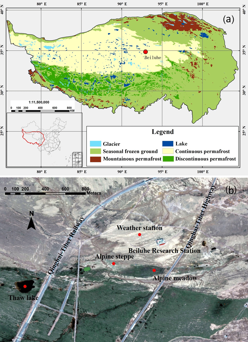
Figure 1Locations of (a) Beiluhe permafrost station on the Qinghai–Tibetan Plateau, and (b) the weather station and the surrounding environment (map data: Google, DigitalGlobe).
2.1 Site description
The site (34∘49′46.2 N, 92∘55′56.58 E, 4628 m a.s.l.) is located in the Beiluhe Basin, in the continuous permafrost region of the central QTP (Fig. 1a, Zou et al., 2017). Based on the map of Li et al. (2015), soils of this region belong to Gelisols and Inceptisols, which occupy 34 % and 28 % of the total area of permafrost region of the QTP. Land surface types include alpine meadow, alpine steppe, barren surface, and thermokarst lakes (Fig. 1b; Lin et al., 2011).
The site is on top of upland plain landforms, which are formed from fluvial and deluvial sediments. The surficial sediments are dominated by fine to gravelly sands and stones (Fig. 2; Yin et al., 2017). Soils at this site are Inceptisols (Wangping Li, Lanzhou University of Technology, personal communication, 18 April 2018) that are commonly underlain by mudstone. The plant community type is mainly alpine meadow, which is dominated by monocotyledonous species, primarily Poaceae and Cyperaceae. The dominant species are Kobresia pygmaea, accompanied by Elymus nutans, Carex moorcroftii, Oxytropis pusilla, Tibetia himalaica, Leontopodium nanum, and Androsace tapete (Fig. 2c–e).
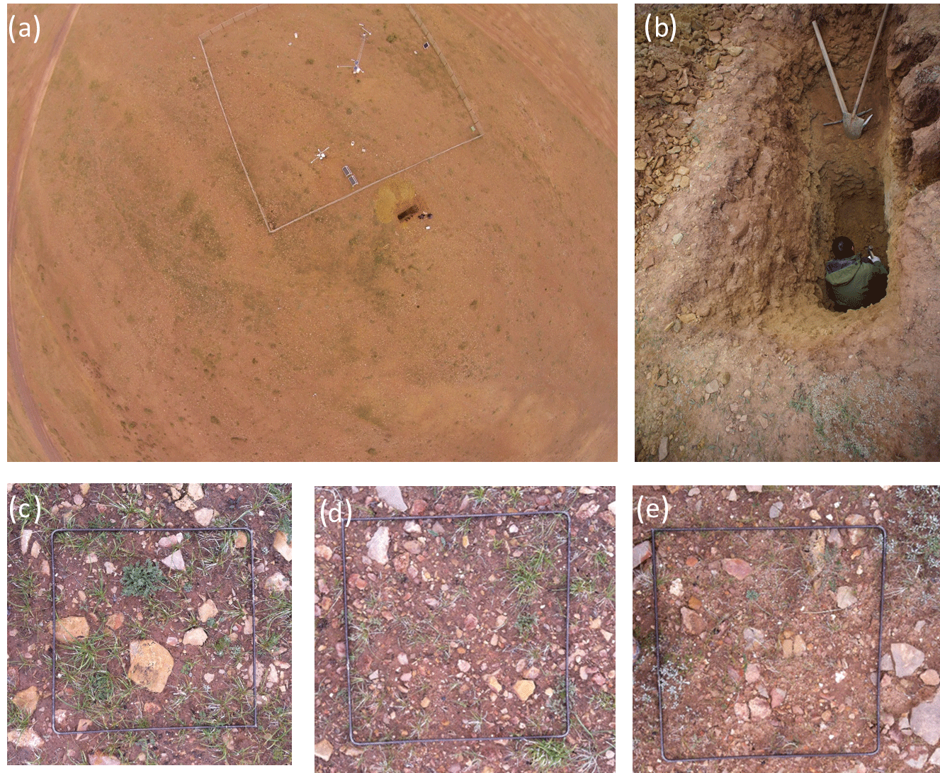
Figure 2Images of site conditions: (a) the aerial view of the weather station and the excavated soil pit (the borehole is located in the lower-left corner of white fence), (b) the detailed view of the excavated soil pit, and (c–e) examples of vegetation, gravel, and stones (iron frame is about 0.5 m × 0.5 m).
A weather station was set up in 2002 (Fig. 2a) to measure air temperature and relative humidity (2.2 m, HMP45C-L11/L36, Campbell Scientific Inc., USA), solar radiation (MS-102, EKO, Japan), and precipitation (QMR102, Vaisala Company, Finland). Soil temperatures were measured at depths of 5, 10, 20, 40, 80, and 160 cm using a PT-100 (EKO, Japan); soil moisture were measured at depths of 20, 40, 80, and 160 cm using a CS616-L50 (EKO, Japan). A CR3000 data logger (Campbell Scientific Inc., USA) was used to store these data at 30 min intervals. These readings were averaged or summed (e.g., precipitation) into monthly values to drive and validate the model. Based on measurements, multi-year mean annual air temperature, precipitation, downward solar radiation, and relative humidity were −3.61 ∘C, 365.7 mm, 206.3 W m−2 and 51.1 % (Fig. 3). The multi-year mean summer (June to August) air temperature and precipitation were 5.27 ∘C and 248.3 mm. The multi-year mean winter (December to February) air temperature and precipitation were −12.44 ∘C and 5.3 mm. The multi-year mean annual, summer, and winter soil temperatures at 40 cm were 0.17, 6.65, and −7.15 ∘C. Those at 80 cm were 0.11, 4.32, and −4.86 ∘C.
A borehole was drilled in 2002, and thermistors made by the State Key Laboratory of Frozen Soil Engineering, Chinese Academy of Sciences were installed at 0.5 m intervals from 0.5 to 10 m, at 2 m intervals from 12 to 30 m, at 4 m intervals from 34 to 50 m,, and at 55 and 60 m. Temperature accuracy of this type of thermistor is ±0.05 ∘C (Wu et al., 2016). The temperatures were recorded on the 5th and 20th days of each month using CR3000 data logger (Campbell Scientific Inc., USA). Based on our measurements, the active layer depth is ∼3.3 m, the depth of zero annual amplitude is ∼6.2 m, and the lower boundary depth of permafrost is at a depth of ∼20 m. The multi-year mean ground temperatures at 0.5, 6, and 60 m are about −0.52, −0.30, and 1.81 ∘C.
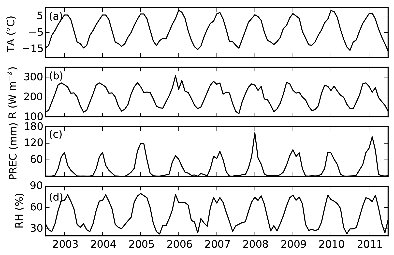
Figure 3Time series of data measured at the Beiluhe weather station, Qinghai–Tibetan Plateau, 2003 to 2011: (a) air temperature (TA, ∘C), (b) downward solar radiation (R, W m−2), (c) precipitation (PREC, mm), and (d) relative humidity (RH, %).
2.2 Soil sampling and measurement
Permafrost dynamics are affected by atmosphere, vegetation, and soil textures; therefore, we excavated soil close to the weather station and borehole (Fig. 2a) down to 2 m (Fig. 2b) in August 2014. We used cut rings (10 cm diameter, 6.37 cm height and 500 cm3) to take soil samples at depth ranges of 0–10, 10–20, 20–30, 40–50, 70–80, 110–120, 150–160, and 190–200 cm. Three replicates were sampled from the top of each depth range and sealed for analysis in the laboratory. Above 120 cm in the soil pit, coarse-soil material was small enough in the cut rings. Below 150 cm, the material is weathered mudstone, which could also be sampled with our cut rings. Based on the excavated soil pit and measured soil temperature, this site is dominated by Inceptisols with the suborder Gelept (soil taxonomy, ST, Soil Survey Staff, 2014). The soil pit consists of A horizon (∼20 cm), Bw horizon (∼20–80 cm) and C material dominated by fractured bedrock.
We used the KD2 Pro (Decagon, US) to measure thermal conductivity of soil samples. The steps we took to determine soil properties for each sample were as follows: (1) the soil sample was dried in an oven and weighed (0.001 g precision) to calculate bulk density; then (2) the soil sample was exposed to a constant temperature (20 ∘C) for 24 h, after which a certain volume of water was injected into the soil samples and a KD2 Pro (Decagon, USA) was used to measure the thermal conductivity; next (3) the sample and the KD2 probe were put into a refrigerator at −15 ∘C for 12 h and thermal conductivity was measured again; (4) steps 2 and 3 were repeated at increasing levels of soil volumetric water content until soil samples were up to the point of saturation; finally, (5) the soil sample was saturated by immersion in water under atmospheric pressure for 24 h and then it was weighed to calculate porosity, and the saturated unfrozen and frozen thermal conductivity were measured accordingly. The bulk density (ρb, g cm−3), porosity (φm, m3 m−3) and volumetric water content (θliq, m3 m−3) were calculated with the following equations:
where mdry, msat, mall, and mcr are masses of oven-dried samples, saturated samples, samples with some water with cut ring, and empty cut ring (g), respectively. Vcr is the volume of the cut ring (cm3). ρw is the density of water (1 g cm−3). We also calculated porosity from bulk density (φc, g m−3):
where ρp is particle density (2.65 g cm−3).
We used pressure membrane instruments (1500F1, Soilmoisture Equipment Corp, US) to measure the matric potential of soil samples (Azam et al., 2014; Wang et al., 2007), using both 15 bar and 5 bar pressure chambers. Pressure values were set to 0, 10, 20, 40, 60, 80, 100, 150, 200, 300, and 400 kpa. It usually took 3–4 days to finish one measurement at one pressure level. We used a soil permeability meter (TST-70, Nanjing T-Bota Scietech Instruments & Equipment Co., Ltd. China) to measure saturated hydraulic conductivity of soil samples (Gwenzi et al., 2011). Finally, soil samples were sieved through a 2.0 mm mesh, and soil particle size distribution was determined with a laser diffraction analyzer (Malvern-2000, Worcestershire, UK).
2.3 Model description
To simulate soil temperatures, soil liquid water content, temperature in rock layers, active layer depth (ALD) and permafrost low boundary depth (PLB) dynamics we used a dynamic organic soil version of the Terrestrial Ecosystem Model (DOS-TEM). Models from the TEM family simulate the carbon and nitrogen pools of vegetation and soil, and their fluxes among atmosphere, vegetation, and soil (McGuire et al., 1992). They have been widely used in studies of cold region ecosystems (e.g., McGuire et al., 2000; Yuan et al., 2012; Zhuang et al., 2004, 2010). The DOS-TEM consists of four modules: environmental, ecological, fire disturbance, and dynamic organic soil (Yi et al., 2010). The environmental module operates on a daily time interval using mean daily air temperature, surface solar radiation, precipitation, and vapor pressure, which are downscaled from monthly input data (Yi et al., 2009a). The module takes into account radiation and water fluxes among the atmosphere, canopy, snowpack, and soil.
2.3.1 Implementation of soil thermal processes
Earlier versions of TEM did not simulate soil temperature (McGuire et al., 1992). Zhuang et al. (2001) incorporated Goodrich (1978) permafrost model into TEM. Yi et al. (2009b) incorporated a two-directional Stefan algorithm to simulate soil freezing and thawing for complex soils with changes in the soil organic and moisture content. Temperatures of all soil layers in the DOS-TEM are updated daily. Phase change is calculated first before heat conduction. A two-directional Stefan algorithm is used to predict the depths of freezing or thawing fronts within the soil (Woo et al., 2004). It first simulates the depth of the front in the soil column from the top downward, using soil surface temperature as the driving temperature. It then simulates the front from the bottom upward using the soil temperature at a specified depth beneath a front as the driving temperature (bottom-up forcing). The latent heat used for phase change is recorded for each soil layer. If a layer contains n freezing or thawing fronts, this layer is then explicitly divided into n+1 soil layers. All soil layers are grouped into three parts: (1) those above the uppermost freezing or thawing front; (2) those below the lowermost freezing or thawing front; and (3) those between the uppermost and lowermost fronts. Soil temperatures are then updated by solving finite difference equations of each part with latent heat from phase change as an energy source or sink (Yi et al., 2014a). Soil surface temperature, which is used as a boundary condition, is calculated using daily air maximum, air minimum, radiation, and leaf area index (Yi et al., 2013).
The version of the DOS-TEM in this study uses the Côté and Konrad (2005) scheme to calculate thermal conductivity (Yi et al., 2013; Pan et al., 2017), which is also been used by other studies on the QTP (e.g., Chen et al., 2012; Luo et al., 2009), and is as follows:
where λ, λsat, λdry are soil thermal conductivity, saturated soil thermal conductivity, and dry soil thermal conductivity (W m−1 K−1), and ke is the Kersten number (Côté and Konrad, 2005). Dry thermal conductivity varies with soil properties according to the following:
where χ (W m−1 K−1) and η (no unit) are parameters accounting for particle shape effects, which are specified for gravel, fine mineral and organic soil (Côté and Konrad, 2005), and φ is porosity. Saturated thermal conductivity varies with water content and phase state according to the following:
where λliq, λice, λs are thermal conductivities of liquid water, ice, and soil solid (W m−1 K−1), which are all constant values. T is soil temperature (∘C) and Tf is the soil freezing point temperature that is assumed to be 0 ∘C in DOS-TEM, which is consistent with most land surface models (e.g., Oleson et al., 2010).
2.3.2 Implementation of soil hydrological processes
Surface runoff, infiltration, and water redistribution among soil layers are simulated in a similar way to the Community Land Model 4 (Oleson et al., 2010). Soil matric potential (Ψ) determines the direction of water movement, and hydraulic conductivity describes the ease with which water can move through the soil.
where Ψsat is the saturated soil matric potential (mm H2O, hereafter mm), and B is the pore size distribution parameter. The soil hydraulic conductivity (K, mm s−1) is a function of the saturated soil hydraulic conductivity (Ksat) as follows:
Several important features relating to permafrost have been considered in the DOS-TEM (see Yi et al., 2014b), including runoff from a perched saturated zone or exchanges of water between the soil and a water reservoir. Runoff from a perched saturated zone above permafrost is implemented following Swenson et al. (2013):
where αis an adjustable parameter (0.6 m−1), Kp is the mean saturated hydraulic conductivity within the perched saturated zone (mm s−1), zfrost and zperched are the depths to the permafrost table and the perched water table (m), and Θ is slope (∘).
The DOS-TEM has been verified against the Neumann equation for water, mineral and organic soil under an idealized condition (Yi et al., 2014b), and validated against field measurements for various locations in Alaska, the Arctic, and the QTP (Yi et al., 2009b, 2013, 2014a).
2.4 Model inputs and initialization
We used the monthly averaged air temperature, downward radiation, precipitation, and humidity as input to drive the DOS-TEM. Leaf area index (LAI), leaf area per unit ground surface area, was specified to be 0.6 m2 m−2 in July and August, 0.1 m2 m−2 in April and October, 0 m2 m−2 between November and March, and interpolated linearly in other months. It is used in the DOS-TEM to calculate ground surface temperature in combination with other meteorological variables (Yi et al., 2013). Its value is unchanged in each month.
Soil temperature and moisture were initialized at −1 ∘C and saturation. The temperature gradient at the bottom of bedrock was set to be 0.06 ∘C cm−1 based on borehole observations. Volumetric unfrozen liquid water in winter was set to be 0.1 based on observations. Multi-year (2003–2012) mean monthly driving data were used to spin up the model for 100 years. In this way, suitable initial values of soil moisture, temperature, and rock temperature of each layer are generated before driving DOS-TEM with monthly data over the period of 2003–2012.
2.5 Sensitivity analyses
The soil textures on the QTP mainly consist of loam, sand, and coarse fragment soils (Wu and Nan, 2016). We used a uniform sand or loam soil profile to represent coarse and fine soil textures, respectively. Sands are the coarsest texture considered in most modeling studies (e.g., Oleson et al., 2010). Therefore, we used our measured parameters to substitute the parameters of sand and loam to investigate the effects of coarse-fragment soil parameters on permafrost dynamics. We first ran DOS-TEM using the default porosity, soil thermal conductivity (Eq. 5), hydraulic conductivity (Eq. 9), and matric potential schemes of these two default soil textures (Eq. 8). The default parameters φ, Ψsat, Ksat and B were calculated based on soil texture used in the Community Land Model 4 (Eqs. 8 and 9; Oleson et al., 2010). We then substituted the default values of φ, Ψsat, Ksat and B based on our laboratory measurements and calibration. Parameters Ψsat and B were fitted with measured matric potential data using Matlab Isqucurvefit tools. We did not calibrate soil thermal conductivity to retrieve parameters of Eqs. (6) and (7). Instead, we interpolated measured thermal conductivities over a range of degrees of saturation (0 to 1), which was used as a look-up table by the DOS-TEM. Therefore, our sensitivity analyses considered a set of four factors, i.e., porosity, matric potential (Ψsat and B), hydraulic conductivity (Ksat and B) and thermal conductivity. We also analyzed three different slope gradients (0, 5, and 10∘) and three different soil thicknesses (3.25, 4.25, and 5.25 m) above 56 m of bed rock. There were 11 soil layers with the top nine layers being 0.05, 0.1, 0.1, 0.2, 0.2, 0.2, 0.3, 0.3, and 0.3 m thick. The thicknesses of the bottom two soil layers were 0.5 and 1 m, 0.5 and 2 m, and 1.5, and 2 m for the 3.25, 4.25, and 5.25 m soil thickness cases. There were six rock layers with thicknesses of 2, 2, 4, 8, 16, and 20 m. Since the site is on the top of an upland plain landform, we did not test the effects of aspect variation. We instead considered the effects of slope on surface runoff. In summary, our sensitivity analyses with the DOS-TEM involved 288 different combinations of parameter values.
We did not measure the heat capacity. The maximum and minimum heat capacities of mineral soil types considered in land surface model are 2.355 and 2.136 MJ m−3, giving a relative difference of less than 10 %. Therefore, in this study, we did not carry out sensitivity tests using thermal diffusivity (the ratio between thermal conductivity and heat capacity).
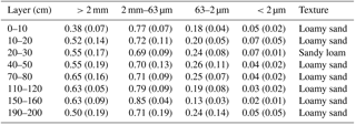
Table 1The mean (standard deviation in brackets) of measured soil bulk density (ρb, g cm−3), porosity calculated from bulk density (φc, m3 mm−3), and measured porosity (φm, m3 m−3) of different layers based on soil samples in this study.
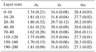
Table 2The particle size diameter fractions (for >2 mm this is the mass ratio between soil particles greater than 2 mm and total soil sample, while for the other fractions this is the ratio between mass of the soil in the size range and the mass of all particles <2 mm) and soil texture (based on USDA classification) of different layers based on soil samples in this study.
3.1 Soil physical properties
3.1.1 Soil porosity, particle size and bulk density
Results from laboratory analysis of the soil samples are shown in Tables 1 and 2. The mean mass ratio of the coarse-soil fraction (particle size diameter >2 mm) of different soil layers ranged from 0.38 to 0.65 with a mean of 0.55. According to the USDA classification system (clay is <2 µm, silt is 2–50 µm, in this study 2–63 µm, and sand is 50 µm −2.0 mm, but in this study was 63 µm −2.0 mm), the major soil texture of this site was loamy sand, with the exception of sandy loam at 20–30 cm depth. The default porosities of sand and loam were 37.3 % and 43.5 %. The φm of samples down to 2 m depth ranged from 21 % to 30 % with a mean of 27 %, and the mean ρb ranged from 1.61 to 1.86 g cm−3 with a mean of 1.74 g cm−3. The φc (Eq. 4) ranged from 29.8 % to 39.2 %. No significant relationships were found among φm, ρb, and the coarse-soil fraction (p>0.05).
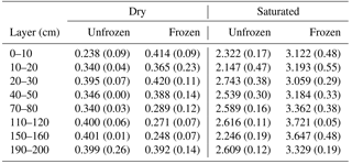
Table 3The mean (standard deviation in brackets) of the measured frozen and unfrozen dry and saturated soil thermal conductivity (W m−1 K−1) of different soil layers.
3.1.2 Thermal conductivity
The results of the thermal conductivity determinations are shown in Table 3. The unfrozen λdry of different soil layers ranged from 0.24 to 0.40 W m−1 K−1 with a mean of 0.36 W m−1 K−1, and the frozen λdry ranged from 0.25 to 0.41 W m−1 K−1 with a mean of 0.35 W m−1 K−1. The difference in λdry between frozen and unfrozen states was small. The unfrozen λsat of different soil layers ranged from 2.15 to 2.74 W m−1 K−1 with a mean of 2.48 W m−1 K−1. The frozen λsat ranged from 3.06 to 3.72 W m−1 K−1 with a mean of 3.33 W m−1 K−1. The difference in λsat between frozen and unfrozen states was about 0.85 W m−1 K−1. There existed a threshold of soil saturation (i.e., ∼0.28 m3 m−3), below which frozen soil thermal conductivity was slightly smaller than unfrozen soil (Fig. 4a).
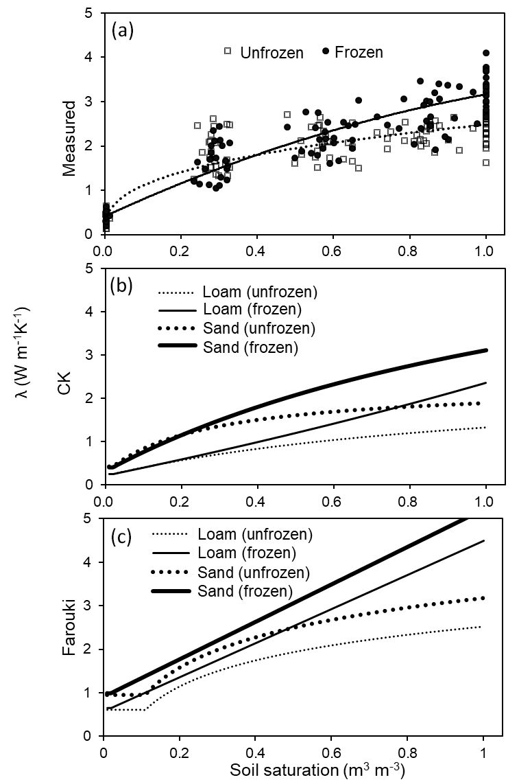
Figure 4The relationship between soil saturation (solid and dotted lines represent frozen and unfrozen cases) and soil thermal conductivity (λ, W m−1 K−1) from (a) measured values (measured; dots and empty diamonds represent measured frozen and unfrozen soil thermal conductivities), (b) using the Côté and Konrad (2005) scheme (CK) and (c) using the Farouki (1986) scheme (Farouki).
Results from determining thermal conductivities using the Côté and Konrad (2005) scheme are shown in Fig. 4b. The default frozen and unfrozen λdry for sand and loam were about 0.42 and 0.24 W m−1 K−1. The frozen and unfrozen λsat of sand were 3.11 and 1.90 W m−1 K−1. Those of loam were about 2.36 and 1.33 W m−1 K−1. Results from determining thermal conductivities using the Farouki (1986) scheme are shown in Fig. 4c. The default frozen and unfrozen λdry for sand and loam were about 0.97 and 0.63 W m−1 K−1. The frozen and unfrozen λsat of sand were 5.21 and 3.18 W m−1 K−1. Those of loam were about 4.49 and 2.52 W m−1 K−1.
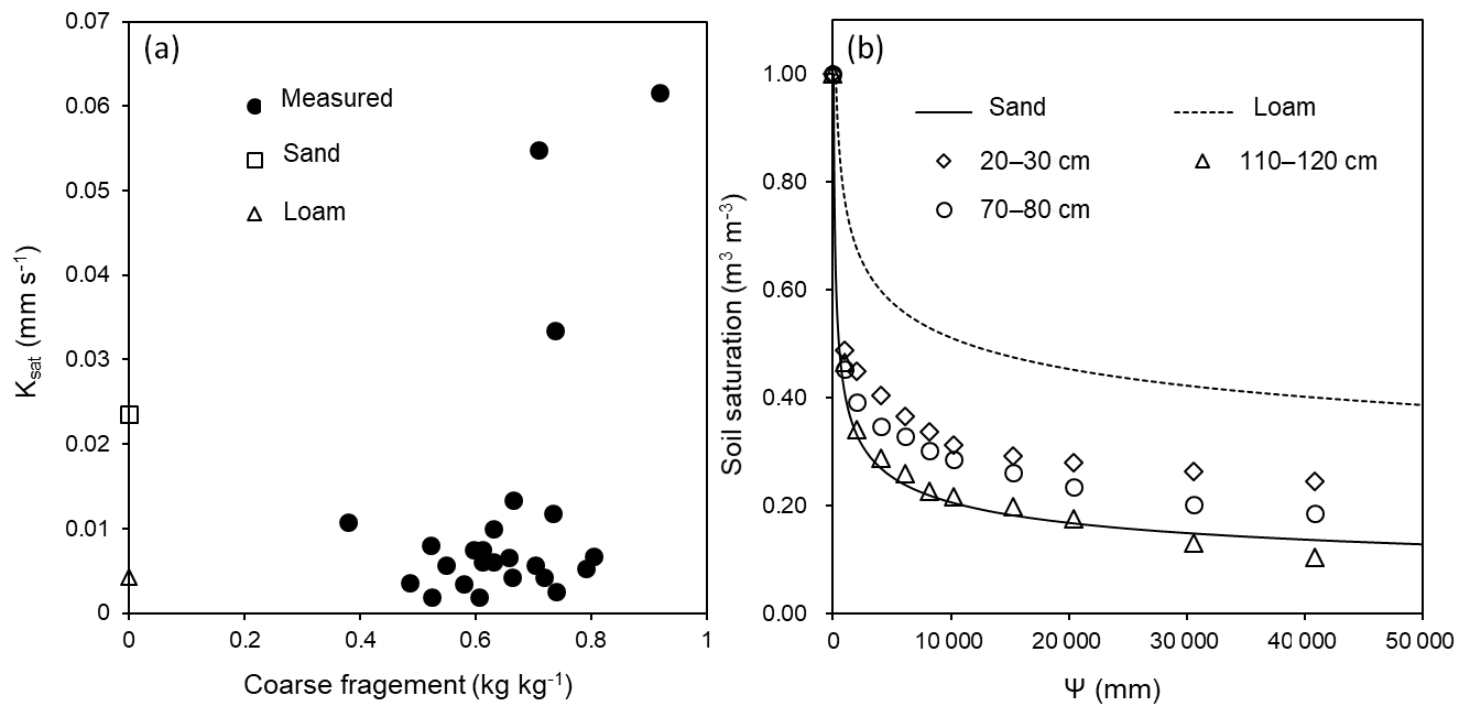
Figure 5The relations between (a) saturated hydraulic conductivity (Ksat, mm s−1) and coarse-fragment fraction (solid dots represent measured values; empty circles and empty triangles represent the corresponding values of sand and loam used in the Community Land Model), and (b) soil saturation (m3 m−3, lines) and absolute value of matric potential (Ψ, mm H2O) at three representative depths (solid and dashed lines represent the default values (Oleson et al., 2010) of sand and loam).
Table 4The mean (standard deviation) of measured saturated hydraulic conductivity (Ksat; mm s−1) and fitted absolute value of saturated matric potential (Ψsat; mm), fitted pore size distribution parameter (B), and the correlation coefficients (R2) between calculated matric potential using fitted and measured equations.
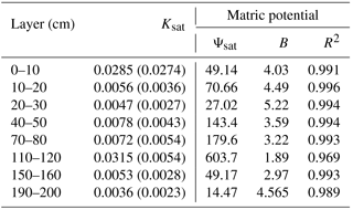
3.1.3 Saturated hydraulic conductivity
The mean Ksat of soil layers, shown in Table 4, ranged from 0.0036 to 0.0315 mm s−1. The maximum Ksat was about 8.7 times larger than the minimum. The Ksat tended to be larger with an increasing proportion of coarse fragment in the soil samples (Fig. 5a), and was about 0.03–0.06 mm s−1 for some samples with coarse fragment greater than 70 %. The default Ksat of sand and loam were 0.024 and 0.0042 mm s−1.
3.1.4 Matric potential
The correlation coefficients between calculated and fitted Ψ, shown in Table 4, were all greater than 0.96. The mean absolute value of Ψsat of soil layers ranged from 14.47 to 603.7 mm, and those of B ranged from 1.89 to 5.22 (Table 4 and Fig. 5b). The default absolute values of Ψsat of sand and loam were 47.29 and 207.34 mm, and the B values were 3.39 and 5.77.
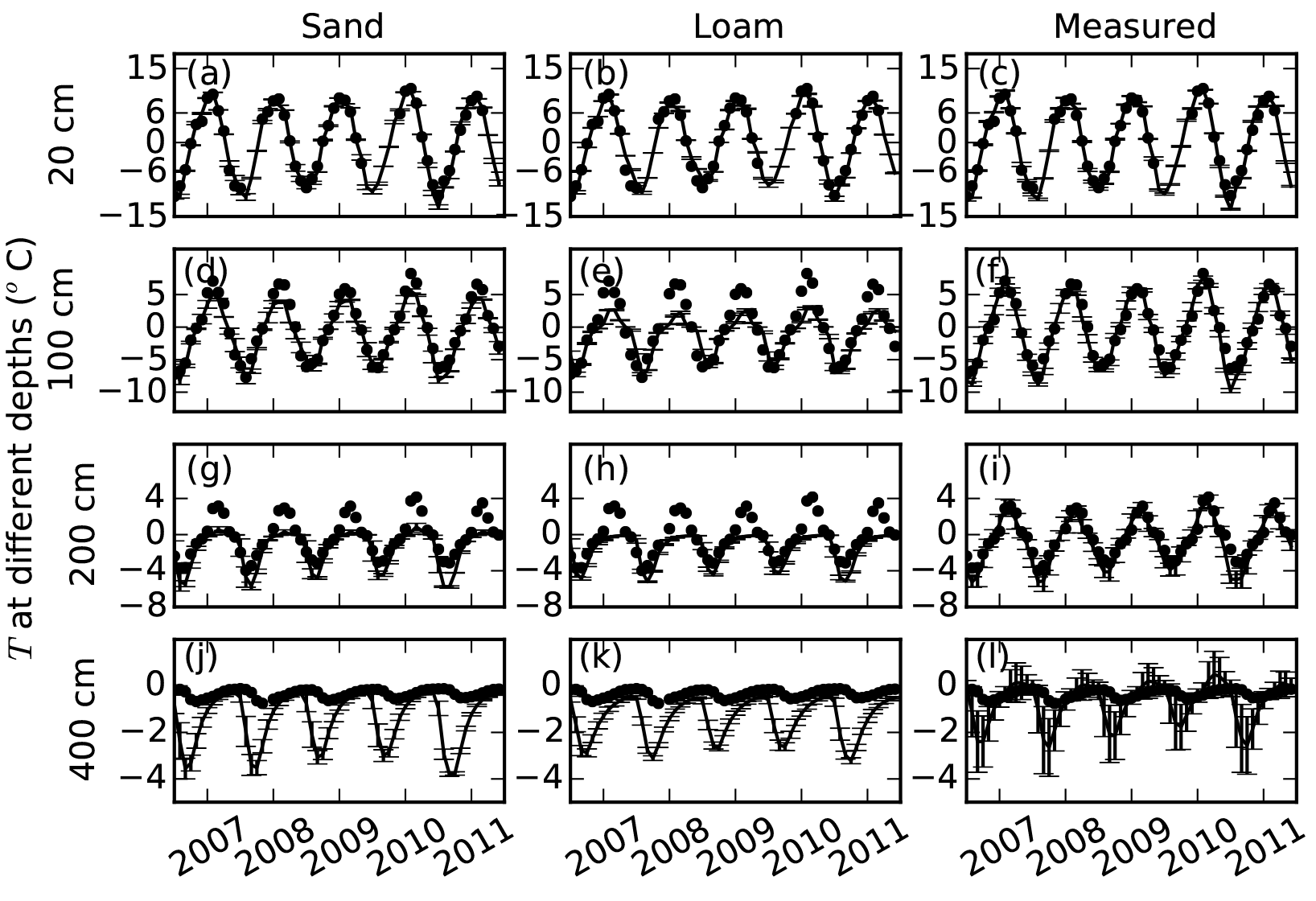
Figure 6Comparisons of soil temperatures (T, ∘C) simulated using default parameters for sand, loam, and our measured parameters (lines) with measured soil temperatures (dots) at 20, 100, 200, and 400 cm depths. Error bars show the standard deviations calculated based on nine simulations with three different slopes and three different soil thicknesses (measured porosities were used in the simulation).
3.2 Comparisons between simulations using default vs. measured parameters
3.2.1 Soil temperature
The mean root mean square errors (RMSEs) between monthly measured soil temperatures and model runs with measured parameters using different combination of soil thicknesses (3.25, 4.25, and 5.25 m) and slopes (0, 5, and 10∘) were about 1.07 ∘C at 20 cm (Fig. 6c). The mean RMSEs for all model runs with default sand and loam parameters were about 0.97 and 1.18 ∘C. For other soil layers, the RMSEs of model runs with measured parameters were much smaller than those with default sand and loam parameters (Fig. 6d–l). The simulated soil temperatures using default sand and loam parameters were all lower than measured ones in summer at 100 and 200 cm, and in winter at 400 cm. The RMSEs can be as large as 2.53 ∘C (Fig. 6e).
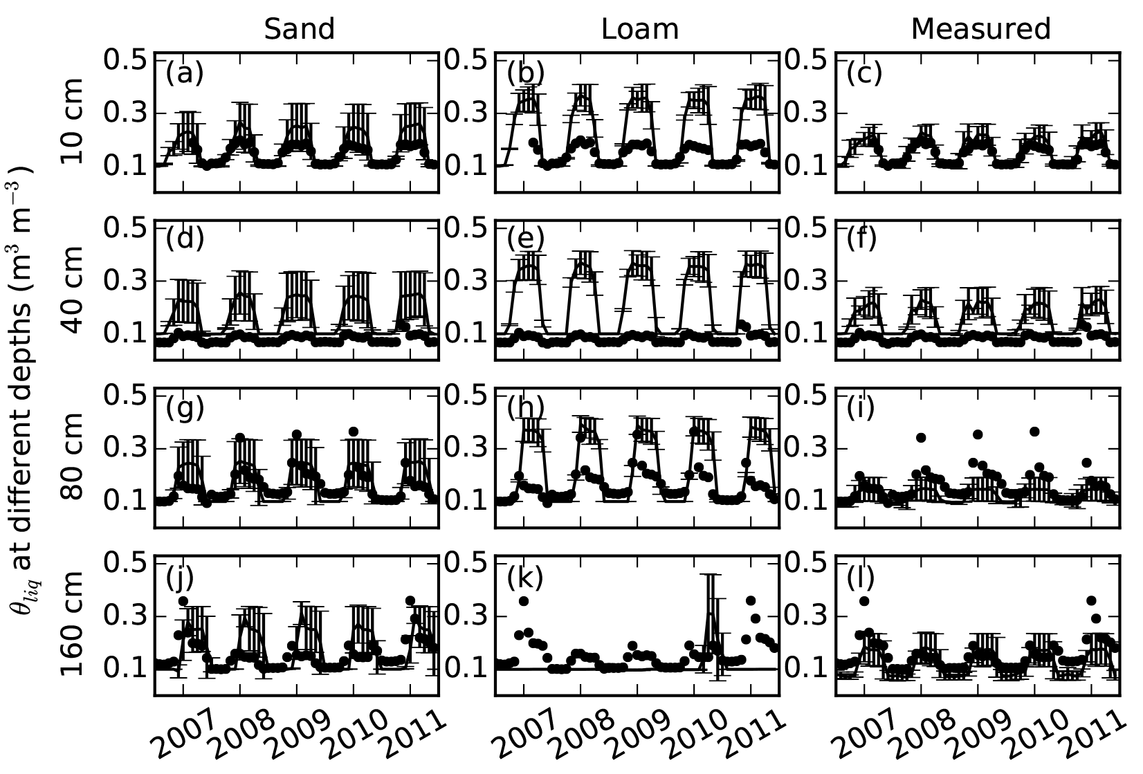
Figure 7Comparisons of soil volumetric liquid water content (θliq, m3 m−3) simulated using default parameters sand, default loam, and measured parameters (lines) with measured soil moisture (dots) at 10, 40, 80, and 160 cm depths. Error bars showed the standard deviation calculated based on nine simulations with three different slopes and three different soil thicknesses (measured porosities were used in the simulation).
The standard deviations of soil temperatures among different slopes and soil thicknesses using measured parameters were larger than those using the default parameters (Fig. 6), and they increased from 0.40 ∘C at 100 cm to 0.61 ∘C at 200 cm (Fig. 6f and i). The standard deviations using default loam parameters were smaller (<0.15 ∘C at all depths) than those using default sand parameters.
3.2.2 Soil liquid water
The mean RMSEs between monthly measured θliq and model simulations with measured parameters ranged from 0.03 to 0.09, which were smaller than RMSEs for sand and loam parameters (Fig. 7). The model simulations for loam parameters have larger RMSEs than those for sand parameters. θliq was always overestimated in warm seasons at depths of 10, 40, and 80 cm. θliq was underestimated at a depth of 160 cm, where the simulated soil was frozen. All model simulations overestimated θliq at 40 cm, where the maximum measured θliq were about 0.1 (Fig. 7d–f).
The standard deviations of θliq among different slopes and soil thicknesses using sand parameters were about 0.077, which were larger than those using measured parameters (∼0.062). The standard deviations of θliq using loam parameters (<0.032) were less than those using measured parameters.
3.2.3 Active layer depth (ALD)
The mean RMSEs between measured ALDs (derived from linear interpolation of soil temperatures) and modeled ALDs (simulated explicitly) were about 1.06, 1.72, and 0.28 m for model runs with sand, loam, and measured parameters (Fig. 8a). The mean standard deviations were about 0.088, 0.026, and 0.28 m. All simulations using sand and loam parameters underestimated ALDs. When φm was replaced with φc, the mean RMSEs and standard deviations were about 0.55 and 0.12 m.
3.2.4 Permafrost lower boundary (PLB)
The mean RMSEs between measured PLBs (derived from linear interpolation of temperatures) and modeled PLBs (derived from linear interpolation of simulated bed rock temperatures) were about 10.25, 10.23, and 6.71 m for model runs with sand, loam, and measured parameters (Fig. 8b). The mean standard deviations were about 1.89, 1.51, and 6.62 m. All simulations using sand and loam parameters overestimated PLBs. When φm was replaced with φc, the mean RMSEs and standard deviations were about 4.78 and 2.82 m.
3.3 Model sensitivity analyses
Deep soil layers used in models are usually specified as being thick. For example, a 1 m thick soil layer was used in our simulations starting around 3 m soil depth. Soil temperatures at this depth are usually close to 0 ∘C. Therefore, the RMSEs of deep soil layers were small and did not facilitate evaluation of model sensitivities. In the following subsections, we used 20 and 100 cm soil temperatures, ALDs and PLBs for sensitivity analysis.
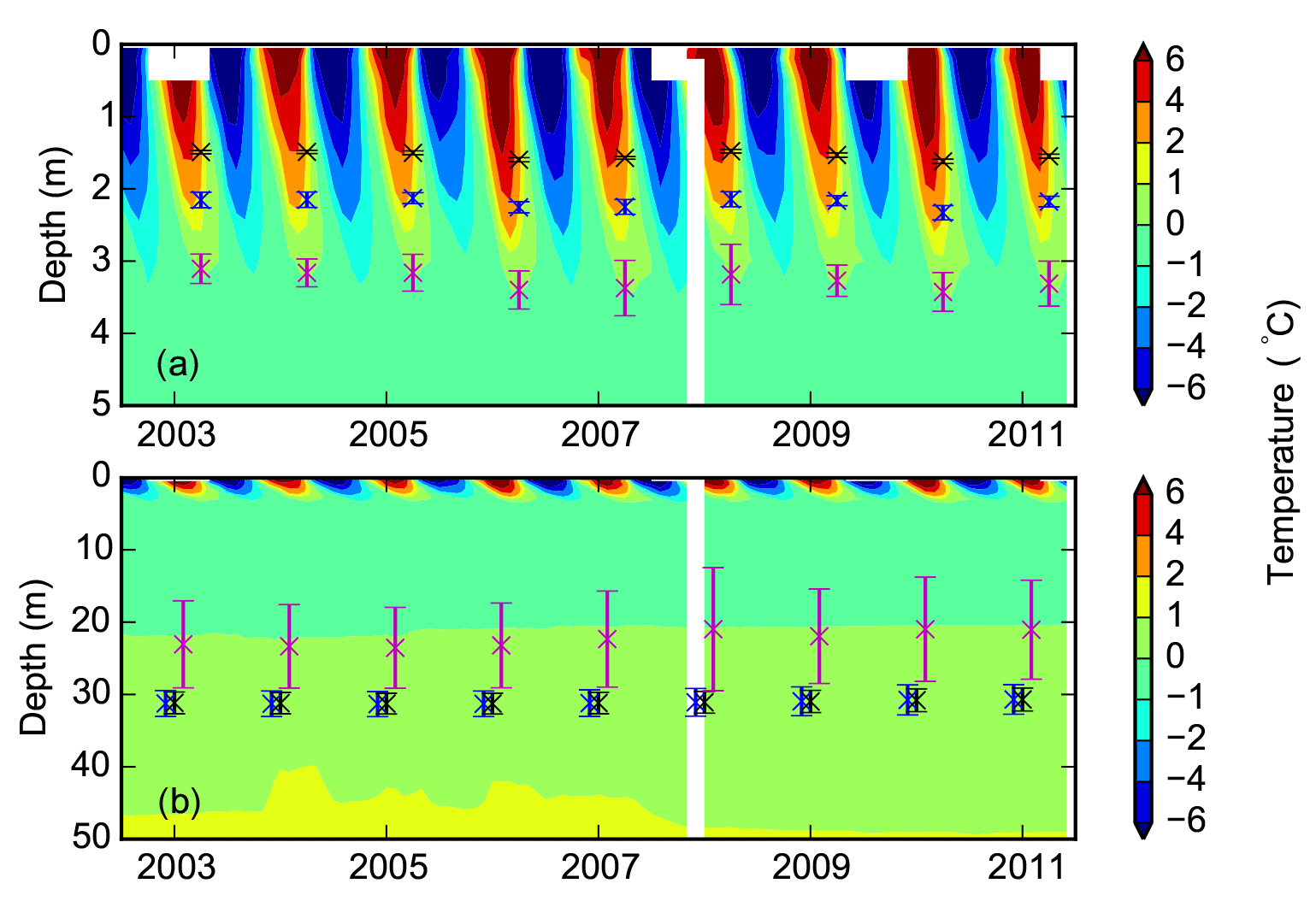
Figure 8Contour plots showing (a) soil temperature (∘C) from borehole measurements down to 5 m superimposed with simulated active layer depths over the period of 2003–2011; and (b) ground temperature down to 50 m superimposed with the simulated permafrost low boundary. Black, blue, and magenta represent simulations with loam, sand, and measured parameters. Error bars show the standard deviation calculated based on nine simulations with three different slopes and three different soil thicknesses (measured porosities were used in the simulation; white zones in the contour plots indicate missing borehole data).

Figure 9Root mean square errors between measurements and model simulations (with different combinations of measured porosity (I), thermal conductivity (II), hydraulic conductivity (III), and matric potential (IV) substituted for default sand parameters) for 20 and 100 cm soil temperatures (∘C), active layer depth (ALD, m), and permafrost low boundary (PLB, m). O and All represent model runs without substitution of default parameters and with all four parameters substituted, respectively. Mean and standard deviation of model simulations with three different soil thicknesses at each slope (0, 5, and 10∘) are shown.
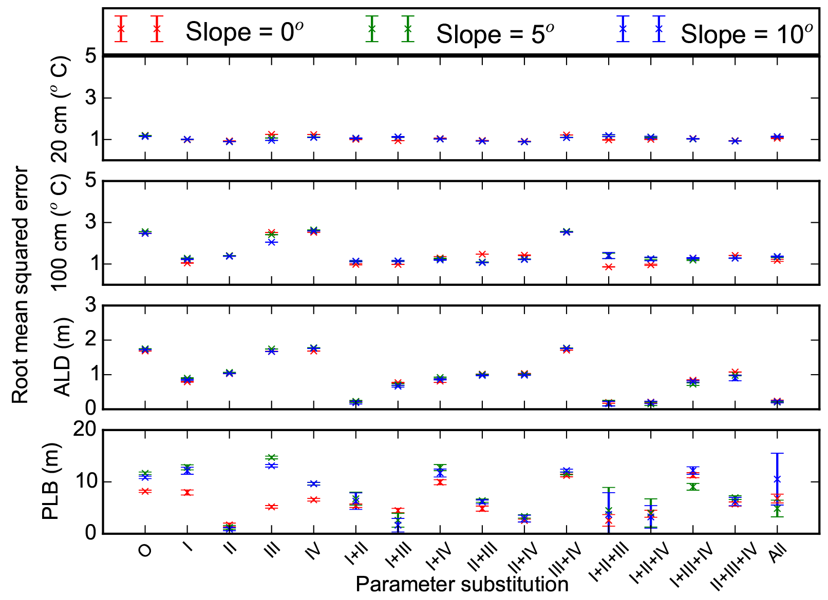
Figure 10Root mean square errors between measurements and model simulations (with different combinations of measured porosity (I), thermal conductivity (II), hydraulic conductivity (III), and matric potential (IV) substituted for default loam parameters) for 20 and 100 cm soil temperatures (∘C), active layer depth (ALD, m), and permafrost low boundary (PLB, m). O and All represent model runs without substitution of default parameters and with all four parameters substituted. Mean and standard deviation of model simulations with three different soil thicknesses at each slope (0, 5, and 10∘) are shown.
3.3.1 Effects of single-parameter sensitivity analyses
Porosity
Replacing default sand or loam porosity with φm changed mean RMSEs of soil temperatures (model runs with three different slopes and three different soil thicknesses at two different soil depths) from 1.18 or 1.84 ∘C to 1.25 or 1.09 ∘C (Figs. 9 and 10). Mean RMSEs of ALD were reduced from 1.06 or 1.72 m to 0.22 or 0.85 m. Mean RMSEs of PLB were changed from 10.26 or 10.24 m to 6.61 or 10.97 m. Mean RMSEs of θliq were reduced from 0.074 or 0.14 to 0.06 or 0.062 when φm was used for replacing default sand or loam porosity (Figs. 11 and 12).
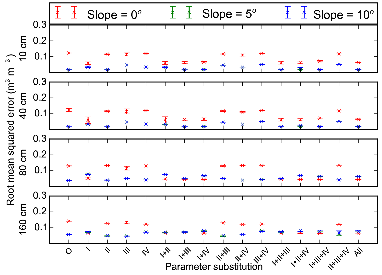
Figure 11Root mean square errors between measurements and model simulations (with different combinations of measured porosity (I), thermal conductivity (II), hydraulic conductivity (III), and matric potential (IV) substituted for default sand parameters) for 10, 40, 80, and 160 cm soil volumetric liquid water content. O and All represent model runs without substitution of default parameters and with all four parameters substituted. Mean and standard deviation of model simulations with three different soil thicknesses at each slope (0, 5, and 10∘) are shown.
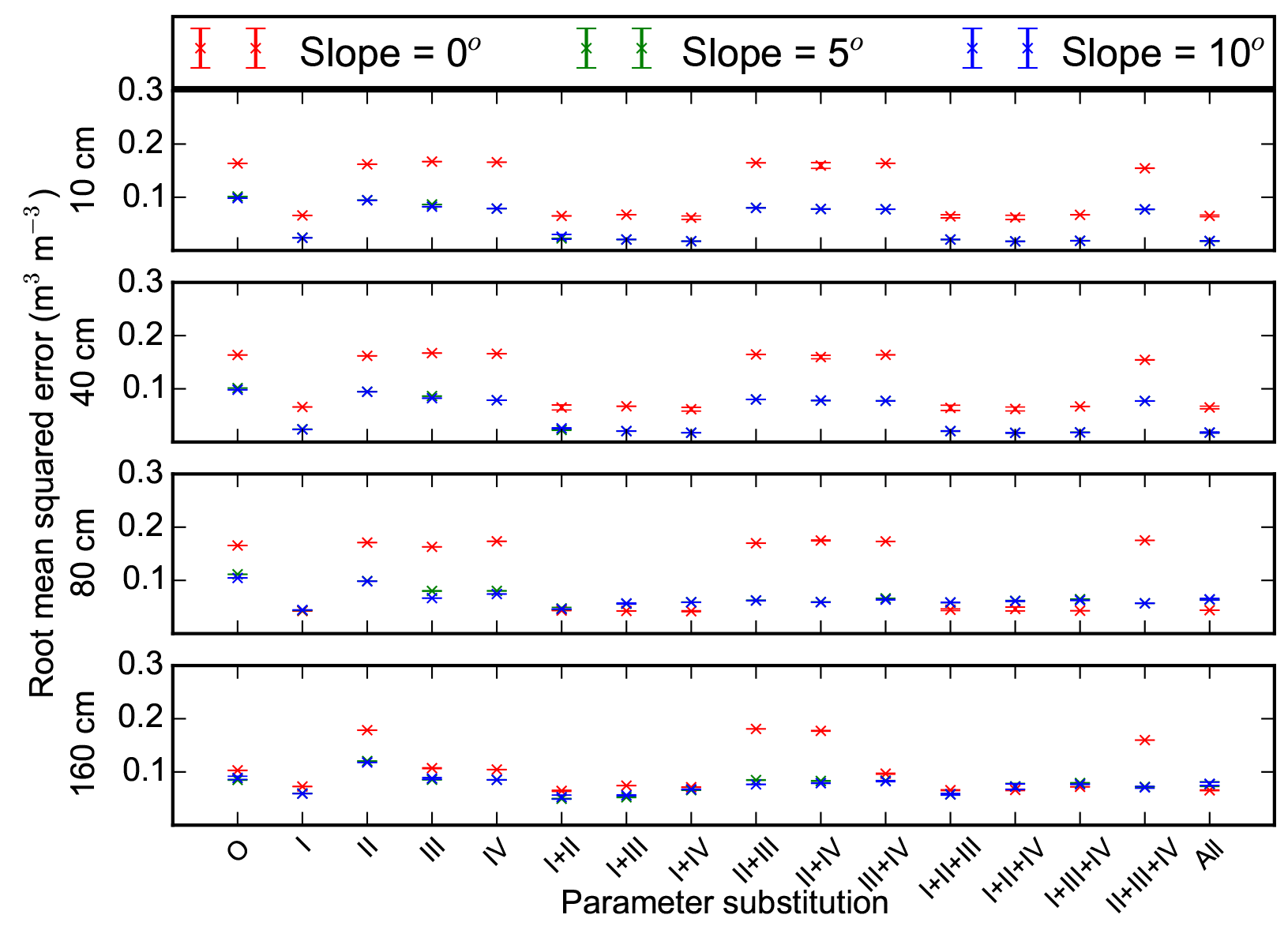
Figure 12Root mean square errors between measurements and model simulations (with different combinations of measured porosity (I), thermal conductivity (II), hydraulic conductivity (III), and matric potential (IV) substituted for default loam parameters) for 10, 40, 80, and 160 cm soil volumetric liquid water content. O and All represent model runs without substitution of default parameters and with all four parameters substituted. Mean and standard deviation of model simulations with three different soil thicknesses at each slope (0, 5, and 10∘) are shown.
Thermal conductivity
Replacing default sand or loam thermal conductivity with measured parameters reduced mean RMSEs of soil temperatures from 1.18 or 1.84 ∘C to 1.02 or 1.15 ∘C (Figs. 9 and 10). Mean RMSEs of ALD were reduced from 1.06 or 1.72 m to 0.56 or 1.04 m. Mean RMSEs of PLB were changed from 10.26 or 10.24 m to 4.18 or 1.27 m. Mean RMSEs of θliq changed very slightly (Figs. 11 and 12).
Hydraulic conductivity and matric potential
Replacing default sand or loam hydraulic conductivity with measured parameters had very small effects on mean RMSEs of soil temperatures and ALDs (Figs. 9 and 10). The same was true for matric potential. When hydraulic conductivity of default sand or loam was substituted, mean RMSEs of PLB decreased or increased, respectively. However, when matric potential was substituted, mean RMSEs of PLBs increased or decreased. When hydraulic conductivity or matric potential parameters were substituted in default sand or loam parameters, mean RMSEs of θliq changed slightly (Figs. 11 and 12).
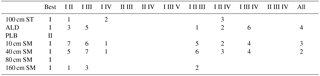
Table 5Model performance when default sand parameters are substituted with combinations of measured porosity (I), thermal conductivity (II), hydraulic conductivity (III), and matric potential (IV).
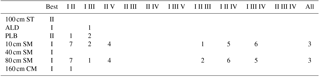
Best column shows the model simulations (individual parameter substitution) with the smallest root mean square error (RMSE) for 100 cm soil temperature (ST, ∘C); active layer depth (ALD, m); permafrost low boundary (PLB, m); 10, 40, 80, and 160 cm soil liquid water content (SM, -). Numbers indicate the combination of parameters that have smaller RMSE than the best model run using individual parameter substitution. The column All indicates the combination of all four parameters. The smallest number indicates the smallest RMSE.
Table 6Model performance when default loam parameters are substituted with combinations of measured porosity (I), thermal conductivity (II), hydraulic conductivity (III), and matric potential (IV).
Best column shows the model simulations (individual parameter substitution) with the smallest root mean square error (RMSE) for 100 cm soil temperature (ST, ∘C); active layer depth (ALD, m); permafrost low boundary (PLB, m); 10, 40, 80, and 160 cm soil liquid water content (SM, -). Numbers indicate the combination of parameters that have smaller RMSE than the best model run using individual parameter substitution. The column All indicates the combination of all four parameters. The smallest number indicates the smallest RMSE.
3.3.2 Effects of combined parameters
We compared model simulations with different combinations of measured parameters (porosity, thermal conductivity, hydraulic conductivity, and matric potential) to those with one substituted measured parameter. We ranked those model runs with less RMSEs than the best of the model runs with one parameter substituted with a measurement-derived value (Tables 5 and 6). We did not consider the 10 cm soil temperature, which was similar across all model runs.
For sand, model simulations with porosity and thermal conductivity and/or hydraulic conductivity substituted had four outcomes with lower RMSEs (Table 5 and Figs. 9 and 11). Only two out of seven outcomes had lower RMSEs with all four parameters substituted. Among all the 18 cases with RMSEs less than the individual “best” RMSE, porosity was included 18 times, and thermal conductivity and hydraulic conductivity were included 10 times.
For loam, model simulations with porosity and thermal conductivity substituted had five outcomes with lower RMSEs (Table 6 and Figs. 10 and 12). Among all the 27 cases with RMSEs less than the individual best RMSE, porosity was included 27 times, thermal conductivity was included 16 times, and matric potential 14 times.
3.3.3 Effects of slope and soil thickness
Changes in slope alone had small effects on simulated soil temperatures and ALDs (Figs. 9 and 10). An increase in slope generally reduced RMSEs of θliq (Figs. 11 and 12). Model simulations with substituted porosity had smaller differences in θliq RMSE between different cases of slopes. For example, the mean RMSEs of model simulations with slopes of 0 or 5∘ and sand parameters substituted with φm were 0.078 or 0.048, while those with porosity not substituted were 0.141 or 0.055. Similarly, the mean RMSEs of model simulations using default loam parameters with porosity substituted were 0.08 or 0.05 for slopes of 0 or 5∘, respectively. The mean RMSEs were 0.18 or 0.1 with porosity not substituted. For a further increase in slope to 10∘, changes of RMSEs of θliq at depths of 10–160 cm were small.
Soil thickness had small effects on 20 and 100 cm soil temperatures and 10–160 cm θliq, and it had prominent effects on PLB for a few cases only with a slope of 10∘ (Figs. 9 and 10).
4.1 Characteristics of soil physical properties
Although the effects of coarse-fragment soils on permafrost dynamics have been considered in a few modeling studies, the thermal and hydraulic properties of coarse-fragment soils were calculated without validation or calibration (Pan et al., 2017; Wu et al., 2018). To our knowledge, this is the first study measuring physical properties of coarse-fragment soil samples from the permafrost region of the QTP.
The weight fraction of coarse fragment (diameter >2 mm, including gravel) in the soil samples we analyzed was greater than 55 % on average, while the typical soil types considered in land surface models and other models usually have much smaller diameter. For comparison, the fractions of gravel considered in Pan et al. (2017) range from 5 % to 33 % and from 10 % to 28 % for the Madoi and Naqu sites. The Beiluhe site and the aforementioned sites are located in regions with Gelisols and Inceptisols, which occupy ∼62 % of the permafrost regions of the QTP (Li et al., 2015). It is possible that coarse-fragment soils commonly exist in the QTP. The data set of Wu and Nan (2016) indicated that gravel content widely exists on the middle and western parts of the QTP. The saturated hydraulic conductivity and matric potential of soil samples measured in this study were more similar to sand than loam (see Sect. 3.1). It is consistent with the study of Wang et al. (2013) that coarse-soil material has a poor water-holding capability.
The measured thermal conductivities of saturated soil samples were relatively close to those estimated by the Côté and Konrad (2005) scheme. However, they were much less than those estimated by the Farouki scheme (Fig. 4). Several other studies also found that Farouki scheme overestimated soil thermal conductivity (Chen et al., 2012; Luo et al., 2009).
One important finding of this study is the relatively small value of porosity. The φm ranged from 0.206 to 0.302, which is less than those of soil types considered in land surface models. For example, the porosities of mineral soil types considered in the Community Land Model range from 0.37 to 0.48 (Oleson et al., 2010). Porosity determines the maximum water stored in a soil layer, and affects soil thermal conductivity, hydraulic conductivity, and matric potential (Eqs. 6–9). It plays a more important role than other parameters in simulated soil thermal and hydrological dynamics (Tables 5 and 6; Figs. 9–12). It is noteworthy that it is easy and efficient to measure porosity.
4.2 Effects of soil water on permafrost dynamics
Soil water not only affects soil thermal properties (e.g., thermal conductivity and heat capacity) but also affects the amount of latent heat lost or gained for freezing or thawing, respectively (Goodrich, 1978; Farouki, 1986). Soil water is determined by infiltration, evapotranspiration, water movement among soil layers, subsurface runoff, and exchange with a water reservoir. Therefore, processes or parameters that affect soil water dynamics will also affect permafrost dynamics. This study quantitatively assessed the effects of soil water on permafrost dynamics. For example, when default loam parameters with high porosity and low saturated hydraulic conductivity were used, soil layers were almost saturated (Fig. 7). The simulated ALDs were about 1.58 m, which was less than half of measured ALDs (Fig. 8a). When the slope was 0∘, subsurface runoff did not occur in the saturated zone above the bottom of the active layer. The simulated θliq was generally higher in the active layer. However, when the slope was 5∘, the simulated θliq was lower and the RMSE was smaller (Figs. 11 and 12). These patterns were especially obvious when both porosity and saturated hydraulic conductivity were large (Eq. 10; Figs. 11 and 12). Other studies have also emphasized the importance of subsurface runoff above the bottom of the active layer (Frey and McClelland, 2009; Walvoord and Striegl, 2007). The effects of soil water content on soil thermal dynamics increased with soil and rock depth (Figs. 9 and 10). The biggest effects were on PLB, which became manifest during long-term spin-up procedures.
Land surface models generally represent soil water dynamics (e.g., Chen et al., 2015; Oleson et al., 2010; Wang et al., 2017). However, the thermal processes in permafrost models usually use specified thermal properties, which were static during model simulations (Li et al., 2009; Nan et al., 2005; Qin et al., 2017; Zou et al., 2017). As shown in this study, variation in soil water content in coarse-fragment soils strongly affects the thermal and hydrological properties; thus it is critical to simulate soil water dynamics to properly project permafrost dynamics in the future.
4.3 Limitations and outlook
4.3.1 Sampling and laboratory measurement
We used cut rings with 10 cm diameter to sample soil and weathered mudstones. However, it is very likely that there could have been much bigger coarse-fragment soils. Therefore, larger containers should be used to take samples for further laboratory analysis in the future.
During our laboratory work, we found two phenomena. First, we used the QL-30 thermophysical instrument (Anter Corporation, US) to measure thermal conductivity. It worked properly in an unfrozen condition. However, when frozen, the surface of the soil sample was usually uneven due to frost heave, which reduces the contact between the QL-30 plate and the soil sample surface. The measured frozen thermal conductivities were smaller than unfrozen thermal conductivity even for the case of saturation, which was definitely wrong. Thus we used the KD2 Pro to determine thermal conductivities. The second phenomenon was that there seems to be a threshold of soil saturation, below which unfrozen soil thermal conductivity is greater than frozen soil thermal conductivity (Fig. 4a). This pattern was somewhat exhibited in estimates of the Côté and Konrad (2005) scheme (Fig. 4b), but not in the estimates of the Farouki scheme (Fig. 4c). More measurements using instruments with higher accuracy should be made in the future.
The measured porosities are generally smaller than those calculated from bulk density. We made additional model simulations using porosities calculated from bulk density in combination with other measured parameters. Our results showed that the RMSEs of ALD and PLB were 0.55 and 4.78 m (figures not shown), whereas those calculated using φm were 0.28 and 6.71 m. There is a variety of methods for measuring soil porosity (Stephens et al., 1998). The method used in this study is widely used for its simplicity (e.g., Chen et al., 2012), and only requires measuring weights of samples under saturation and dry conditions (Eq. 2). Though soil samples were immersed in water under atmospheric pressure for 24 h to research saturation, it is possible that some air still remained in the soil after immersion but most of our soil samples contained coarse fragments and we assumed the volume of any remaining air to be negligible.
4.3.2 Model simulation
Although the DOS-TEM using measured parameters provided satisfactory results, there are some aspects requiring further improvement in the future. For example, the measured soil moisture at 40 cm depth was less than 0.1 m3 m−3. However, the simulated soil moisture were always much greater (Fig. 7f). There were also spikes in measured soil moisture at 80 and 160 cm depths, which were not presented in the simulation (Fig. 7i and l). In the DOS-TEM, the unfrozen soil water content, or super-cold water, was prescribed to be 0.1 m3 m−3. When soil is freezing, if the soil liquid water content is lower than this value, no phase change will happen (Fig. 7k). Therefore, model results would improve with the capability to simulate the dynamics of unfrozen soil water content (Romanovsky and Osterkamp, 2000).
The TEM family models use monthly atmospheric data to drive both site and regional applications. In this study, 30 min and daily driving data are available. Although it is possible to lose fidelity after daily interpolations, we still decided to use monthly driving data for the following reasons: (1) Zhuang et al. (2001) performed a test with daily and monthly driving data sets, and the results showed that the RMSEs of ALD were about 3 cm; and (2) we intend to apply the model over large regions where reliable daily data sets might not be available.
4.3.3 Regional applications
The coarse-fragment content of soil affects its physical properties. For example, soil porosity and saturated hydraulic conductivity are determined by the fraction of gravel, diameter, and degree of mixture (Zhang et al., 2011). Thus soil texture plays an important role in permafrost dynamics (Fig. 8). The dominant soil textures on the QTP from Wu and Nan (2016) are loam, sand, and gravel. The specification of loam in simulations results in estimates of ALD that are much smaller than the measurements (Yi et al., 2014a). To properly simulate the distribution and dynamics of permafrost on the QTP under climate change scenarios, it is important to develop proper schemes of soil physical properties in relation to coarse-fragment content (including gravel) and to develop regional data sets of soil texture for input.
Organic soil carbon content in mineral soil on the QTP affects soil porosity and thermal conductivity (Chen et al., 2012). However, in the site considered in this study, the amount of organic soil carbon in the soil was small (Fig. 2), and we did not explicitly consider the effects of organic soil carbon on soil properties. Alpine swamp meadow, alpine meadow, alpine steppe, and alpine desert are the major vegetation types on the QTP (Wang et al., 2016; see also Fig. 1b). Alpine swamp meadow and alpine meadow usually contain fine soil particles and high organic carbon density, while the other two types usually contain coarse-soil particle and low organic carbon density (Qin et al., 2015). More laboratory work is needed to develop proper schemes for representing mixed soil with fine mineral, coarse fragment (including gravel), and organic carbon in permafrost models. It is the first priority to develop schemes that make use of porosity data sets due to its importance and simplicity of measurement.
The development of a spatially explicit data set of soil texture is also required for regional projections of permafrost changes on the QTP. Currently, a preliminary data set for gravel exists (Wu and Nan, 2016), though gravel soil has only been mentioned in a few papers on the QTP (Chen et al., 2015; Wang et al., 2011; Yang et al., 2009). One way to improve the regional data set is to collect relevant data through extensive field campaigns (e.g., Li et al., 2015). Ground-penetrating radar is a feasible tool that retrieves soil thickness above the coarse-fragment soil layer (Han et al., 2016), and coarse-fragment soils can be identified in photos taken with unmanned aerial vehicles (Chen et al., 2017; Yi, 2017). In combination with ancillary data sets (e.g., geomorphology, topography, vegetation), it is possible to improve the accuracy of spatial data sets of soil texture on the QTP (Li et al., 2015; Wu et al., 2016). Another way is to retrieve soil physical properties using data assimilation technology, as done by Yang et al. (2016), who assimilated porosity using a land surface model and microwave data.
In this study, we excavated soil samples from a permafrost site on the central QTP and measured soil physical properties in the laboratory. Coarse fragments were common in the soil profile (up to 65 % of soil mass) and porosity was much smaller than the typical soil types used in land surface models. We then performed a sensitivity analysis of these parameters on soil thermal and hydrological processes within a terrestrial ecosystem model. When default sand or loam parameters were substituted with measured soil properties, the model errors of active layer depth were reduced by 74 % or 84 %, whereas those of the low permafrost boundary were reduced by 35 % or 34 %. Our sensitivity analyses showed that porosity played a more important role in reducing model errors than the other soil properties examined. Though it is unclear how representative this soil is in the QTP, it is clear that soil physical properties specific to the QTP should be used to properly project permafrost dynamics into the future.
The laboratory data set is included in Tables 1–4. Any other specific data can be provided by the authors on request.
YD and QW designed the study, JC, YQ and SY collected the soil samples, and YH and XG performed laboratory measurements. SY did modeling work. All authors contributed to the discussion of the results. SY led the writing of the paper and all co-authors contributed to it.
The authors declare that they have no conflict of interest.
We would like to thank Dave McGuire of University of Alaska Fairbanks
for his careful editing; Yi Sun for vegetation classification; Xia
Cui of Lanzhou University, Guangyue Liu for determining depth of zero
annual amplitude, Yan Qin for measurements of soil particle size
distribution; Chien-Lu Ping of University of Alaska and Wangping
Li of Lanzhou University of Technology for helping on soil taxonomy; and the
editor and two anonymous reviewers for valuable comments. This study was
jointly supported through grants provided as part of the National Natural
Science Foundation Commission (41422102, 41690142, and 41730751), and the
independent grants from the State Key Laboratory of Cryosphere Sciences
(SKLCS-ZZ-2018).
Edited by: Peter Morse
Reviewed by: two anonymous referees
Anisimov, O. A.: Potential feedback of thawing permafrost to the global climate system through methan emission, Environ. Res. Lett., 2, 045016, https://doi.org/10.1088/1748-9326/2/4/045016, 2007.
Arocena, J., Hall, K., and Zhu, L. P.: Soil formation in high elevation and permafrost areas in the Qinghai Plateau (China), Span. J. Soil Sci., 2, 34–49, 2012.
Azam, G., Grant, C. D., Murray, R. S., Nuberg, I. K., and Misra, R. K. : Comparison of the penetration of primary and lateral roots of pea and different tree seedlings growing in hard soils, Soil Res., 52, 87–96, 2014.
Boike, J., Kattenstroth, B., Abramova, K., Bornemann, N., Chetverova, A., Fedorova, I., Fröb, K., Grigoriev, M., Grüber, M., Kutzbach, L., Langer, M., Minke, M., Muster, S., Piel, K., Pfeiffer, E.-M., Stoof, G., Westermann, S., Wischnewski, K., Wille, C., and Hubberten, H.-W.: Baseline characteristics of climate, permafrost and land cover from a new permafrost observatory in the Lena River Delta, Siberia (1998–2011), Biogeosciences, 10, 2105–2128, https://doi.org/10.5194/bg-10-2105-2013, 2013.
Chen, H., Nan, Z., Zhao, L., Ding, Y., Chen, J., and Pang, Q.: Noah Modelling of the Permafrost Distribution and Characteristics in the West Kunlun Area, Qinghai-Tibet Plateau, China, Permafr. Periglac., 26, 160–174, 2015.
Chen, J., Yi, S., and Qin, Y.: The contribution of plateau pika disturbance and erosion on patchy alpine grassland soil on the Qinghai-Tibetan Plateau: Implications for grassland restoration, Geoderma, 297, 1–9, 2017.
Chen, Y., Yang, K., Tang, W., Qin, J., and Zhao, L.: Parameterizing soil organic carbon's impacts on soil porosity and thermal parameters for Eastern Tibet grasslands, Sci. China Ser. D, 55, 1001–1011, 2012.
Côté, J. and Konrad, J.: A generalized thermal conductivity model for soils and construction materials, Can. Geotech. J., 42, 443–458, 2005.
Du, Z., Cai, Y., Yan, Y., and Wang, X.: Embedded rock fragments affect alpine steppe plant growth, soil carbon and nitrogen in the northern Tibetan Plateau, Plant. Soil, 420, 79–92, 2017.
Farouki, O. T.: Thermal properties of soils, Cold Reg. Res. Eng. Lab., Hanover, N. H, 1986.
Fox, J. D.: Incorporating Freeze-Thaw Calculations into a water balance model, Water Resour. Res., 28, 2229–2244, 1992.
Frey, K. E. and McClelland, J. W.: Impacts of permafrost degradation on arctic river biogeochemistry, Hydrol. Process., 23, 169–182, 2009.
Goodrich, E. L.: Efficient Numerical Technique for one-dimensional Thermal Problems with phase change, Int. J. Heat Mass Transf., 21, 615–621, 1978.
Gwenzi, W., Hinz, C., Holmes, K., Phillips, I. R., and Mullins, I. J.: Field-scale spatial variability of saturated hydraulic conductivity on a recently constructed artificial ecosystem, Geoderma, 166, 43–56, 2011.
Han, X., Liu, J., Zhang, J., and Zhang, Z.: Identifying soil structure along headwater hillslopes using ground penetrating radar based technique, J. Mount. Sci., 13, 405–415, 2016.
Jorgenson, M. T., Shur, Y. L., and Pullman, E. R.: Abrupt increase in permafrost degradation in Arctic Alaska, Res. Lett., 33, L02503, https://doi.org/10.1029/2005GL024960, 2006.
Langer, M., Westermann, S., Heikenfeld, M., Dorn, W., and Boike, J.: Satellite-based modeling of permafrost temperatures in a tundra lowland landscape, Remote Sens. Environ., 135, 12–24, 2013.
Li, J., Sheng, Y., Wu, J., Chen, J., and Zhang, X.: Probability distribution of permafrost along a transportation corridor in the northeastern Qinghai province of China, Cold Reg. Sci. Technol., 59, 12–18, 2009.
Li, W., Zhao, L., Wu, X., Zhao, Y., Fang, H., and Shi, W.: Distribution of soils and landform relationships in the permafrost regions of Qinghai-Xizang (Tibetan) Plateau, Chinese Sci. Bull., 23, 2216–2226, 2015.
Lin, Z., Niu, F., Liu, H., and Lu, J.: Hydrothermal processes of alpine tundra lakes, Beiluhe Basin, Qinghai-Tibet Plateau, Cold Reg. Sci. Techol., 65, 446–455, 2011.
Luo, S., Lv, S., Zhang, Y., Hu, Z., Ma, Y., Li, S., and Shang, L.: Soil thermal conductivity parameterization establishment and application in numerical model of central Tibetan Plateau, China J. Geophys., 52, 919–928, 2009 (in Chinese with English Abstract).
McGuire, A. D., Melillo, J., Jobbagy, E. G., Kicklighter, D., Grace, A. L., Moore, B., and Vorosmarty, C. J.: Interactions Between Carbon and Nitrogen Dynamics in Estimating Net Primary Productivity for Potential Vegetation in North America, Global Biogeochem. Cy., 6, 101–124, 1992.
McGuire, A. D., Clein, J. S., Melillo, J., Kicklighter, D., Meier, R. A., Vorosmarty, C. J., and Serreze, M. C.: Modelling carbon responses of tundra ecosystems to historical and projected climate: sensitivity of pan-Arctic carbon storage to temporal and spatial variation in climate, Global Change Biol., 6 (Suppl. 1), 141–159, 2000.
McGuire, A. D., Anderson, L. G., Christensen, T. R., Dallimore, S., Guo, L., Hayes, D. J., and Roulet, N.: Sensitivity of the carbon cycle in the Arctic to climate change, Ecol. Monogr., 79, 523–555, 2009.
Nan, Z., Li, S., and Cheng, G.: Prediction of permafrost distribution on the Qinghai-Tibet Plateau in the next 50 and 100 years, Sci. China Ser. D, 48, 797–804, 2005.
Nelson, F. E., Anisimov, O. A., and Shiklomanov, N. I.: Subsidence risk from thawing permafrost, Nature, 410, 889–890, 2001.
Oleson, K. W., Lawrence, D. M., Bonan, G. B., Flanner, M. G., Kluzek, E., Lawrence, P. J., Levis, S., Swenson, S. C., and Thornton, P.: Technical description of version 4.0 of the Community Land Model (CLM), University Corporation for Atmospheric Research, NCAR 2153-2400, 2010.
Pan, Y., Lv, S., Li, S., Gao, Y., Meng, X., Ao, Y., and Wang, S.: Simulating the role of gravel in freeze–thaw processon the Qinghai–Tibet Plateau, Theor. Appl. Climatol., 127, 1011–1022, 2017.
Qin, Y., Yi, S., Chen, J., Ren, S., and Ding, Y.: Effects of gravel on soil and vegetation properties of alpine grassland on the Qinghai-Tibetan plateau, Ecol. Eng., 74, 351–355, 2015.
Qin, Y., Wu, T. , Zhao, L., Wu, X., Li, R., Xie, C., Pang, Q., Hu, G., Qiao, Y., Zhao, G., Liu, G., Zhu, X., and Hao, J.: Numerical Modeling of the Active Layer Thickness and Permafrost Thermal State Across Qinghai-Tibetan Plateau, J. Geophys. Res.-Atmos., 21, 11604–11620, https://doi.org/10.1002/2017JD026858, 2017.
Romanovsky, V. E. and Osterkamp, T. E.: Effects of unfrozen water on heat and mass transport processes in the active layer and permafrost, Permafr. Periglac., 11, 219–239, 2000.
Salmon, V. G., Soucy, P., Mauritz, M., Celis, G., Natali, S. M., Mack, M. C., and Schuur, E. A.: Nitrogen availability increases in a tundra ecosystem during five years of experimental permafrost thaw, Global Change Biol., 22, 1927–1941, 2015.
Soil Survey Staff: Keys to Soil Taxonomy, 12th Ed., USDA-Natural Resources Conservation Service, Washington, DC, 2014.
Stephens, D. B., Hsu, K., Prieksat, M. A., Ankeny, M. D., Blandford, N., Roth, T. L., Kelsey, J. A., and Whitworth, J. R.: A comparison of estimated and calculated effective porosity, Hydrol. Process., 6, 156–165, 1998.
Swenson, S. C., Lawrence, D. M., and Lee, H.: Improved simulation of the terrestrial hydrological cycle in permafrost regions by the Community Land Model, J. Adv. Model. Earth Syst., 4, M08002, https://doi.org/10.1029/2012MS000165, 2013.
Walvoord, M. A. and Striegl, R. G.: Increased groundwater to stream discharge from permafrost thawing in the Yukon River basin: Potential impacts on lateral export of carbon and nitrogen, Geophys. Res. Lett., 34, L12402, https://doi.org/10.1029/2007GL030216, 2007.
Wang, F. X., Kang, Y., Liu, S. P., and Hou, X. Y.: Effects of soil matric potential on potato growth under drip irrigation in the North China Plain, Agr. Water Manage., 88, 34–42, 2007.
Wang, G., Li. Y., Wang. Y., and Wu, Q.: Effects of permafrost thawing on vegetation and soil carbon pool losses on the Qinghai-Tibet Plateau, China, Geoderma, 143, 143–152, 2008.
Wang, H., Xiao, B., Wang, M., and Shao, M.: Modeling the soil water retention curves of soil-gravel mixtures with regression method on the Loess Plateau of China, PLoS ONE, 8, e59475, https://doi.org/10.1371/journal.pone.0059475, 2013.
Wang, L., Zhou, J., Qi, J., Sun, L., Yang, K., Tian, L., and Koike, T.: Development of a land surface model with coupled snow and frozen soil physics, Water Resour. Res., 53, 5085–5103, https://doi.org/10.1002/2017WR020451, 2017.
Wang, X., Liu, G., and Liu, S.: Effects of gravel on grassland soil carbon and nitrogen in the arid regions of the Tibetan Plateau, Geoderma, 166, 181–188, 2011.
Wang, Z., Wang, Q., Zhao, L., Wu, X., Yue, G., Zou, D., Nan, Z., Liu, G., Pang, Q., Fang, H., Wu, T., Shi, J., Jiao, K., Zhao, Y., and Zhang, L.: Mapping the vegetation distribution of the permafrost zone on the Qinghai-Tibet Plateau, J. Mountain Sci., 13, 1035–1046, 2016.
Woo, M. K., Arain, M. A., Mollinga, M., and Yi, S.: A two-directional freeze and thaw algorithm for hydrologic and land surface modelling, Geophys. Res. Lett., 31, L12501, https://doi.org/10.1029/2004GL019475, 2004.
Wright, N., Hayashi, M., and Quinton, W. L.: Spatial and temporal variations in active layer thawing and their implication on runoff generation in peat-covered permafrost terrain, Water Resour. Res., 45, W05414, https://doi.org/10.1029/2008WR006880, 2009.
Wu, Q. and Zhang, T.:. Changes in active layer thickness over the Qinghai-Tibetan Plateau from 1995 to 2007, J. Geophys. Res., 115, D09107, https://doi.org/10.1029/2009JD012974, 2010.
Wu, Q., Cheng, G., and Ma, W.: Impact of permafrost change on the Qinghai-Tibet Railroad engineering, Sc. China Ser. D, 47, 122–130, 2004.
Wu, Q., Zhang, Z., Gao, S., and Ma, W.: Thermal impacts of engineering activities and vegetation layer on permafrost in different alpine ecosystems of the Qinghai-Tibet Plateau, China, The Cryosphere, 10, 1695–1706, https://doi.org/10.5194/tc-10-1695-2016, 2016.
Wu, X. and Nan, Z.: A Multilayer Soil Texture Dataset for Permafrost Modeling over Qinghai – Tibetan Plateau, IGARSS, 4917–4920, 2016.
Wu, X., Zhao, L., Fang, H., Zhao, Y., Smoak, J. M., Pang, Q., and Ding, Y.: Environmental controls on soil organic carbon and nitrogen stocks in the high-altitude arid western Qinghai-Tibetan Plateau permafrost region, J. Geophys. Res., 121, 176–187, 2016.
Wu, X., Nan, Z., Zhao, S., Zhao, L., and Cheng, G.: Spatial modeling of permafrost distribution and properties on the Qinghai-Tibetan Plateau, Permafr. Periglac., 29, 86–99, https://doi.org/10.1002/ppp.1971, 2018.
Yang, J., Mi, R., and Liu, J.:Variations in soil properties and their effect on subsurface biomass distribution in four alpine meadows of the hinterland of the Tibetan Plateau of China, Environ. Geol., 57, 1881–1891, 2009.
Yang, K., Zhu, L., Chen, Y., Zhao, L., Qin, J., Lu, H., and Fang, N.: Land surface model calibration through microwave data assimilation for improving soil moisture simulations, J. Hydrol., 533, 266–276, 2016.
Ye, B., Yang, D., Zhang, Z., and Kane, D. L.: Variation of hydrological regime with permafrost coverage over Lena Basin in Siberia, J. Geophys. Res., 114, D07102, https://doi.org/10.1029/2008JD010537, 2009.
Yi, S.: FragMAP: a tool for long-term and cooperative monitoring and analysis of small-scale habitat fragmentation using an unmanned aerial vehicle, Int. J. Remote Sens., 38, 2686–2697, 2017.
Yi, S., Manies, K. L., Harden, J., and McGuire, A. D.: The characteristics of organic soil in black spruce forests: Implications for the application of land surface and ecosystem models in cold regions, Geophys. Res. Lett., 36, L05501, https://doi.org/10.1029/2008GL037014, 2009a.
Yi, S., McGuire, A. D., Harden, J., Kasischke, E., Manies, K. L., Hinzman, L. D., Liljedahl, A., Randerson, J. T., Liu, H., Romanovsky, V. E., Marchenko, S., and Kim, Y.: Interactions between soil thermal and hydrological dynamics in the response of Alaska ecosystems to fire disturbance, J. Geophys. Res., 114, G02015, https://doi.org/10.1029/2008JG000841, 2009b.
Yi, S., McGuire, A. D., Kasischke, E., Harden, J., Manies, K. L., Mack, M., and Turetsky, M. R.: A Dynamic organic soil biogeochemical model for simulating the effects of wildfire on soil environmental conditions and carbon dynamics of black spruce forests, J. Geophys. Res., 115, G04015, https://doi.org/10.1029/2010JG001302, 2010.
Yi, S., Li, N., Xiang, B., Ye, B., and McGuire, A.D.: Representing the effects of alpine grassland vegetation cover on the simulation of soil thermal dynamics by ecosystem models applied to the Qinghai-Tibetan Plateau, J. Geophys. Res., 118, 1–14, https://doi.org/10.1002/jgrg.20093, 2013.
Yi, S., Wang, X., Qin, Y., Xiang, B., and Ding, Y.: Responses of alpine grassland on Qinghai–Tibetan plateau to climate warming and permafrost degradation: a modeling perspective, Environ. Res. Lett., 9, 074014, https://doi.org/10.1088/1748-9326/9/7/074014, 2014a.
Yi, S., Wischnewski, K., Langer, M., Muster, S., and Boike, J.: Freeze/thaw processes in complex permafrost landscapes of northern Siberia simulated using the TEM ecosystem model: impact of thermokarst ponds and lakes, Geosci. Model Dev., 7, 1671–1689, https://doi.org/10.5194/gmd-7-1671-2014, 2014b.
Yin, G., Niu, F., Lin, Z., Luo, J., and Liu, M.: Effects of local factors and climate on permafrost conditions and distribution in Beiluhe basin, Qinghai-Tibet Plateau, China, Sci. Total Environ., 581–582, 472–485, 2017.
Yuan, F. M., Yi, S. H., McGuire, A. D., Johnson, K. D., Liang, J., Harden, J. W., and Kurz, W. A.:Assessment of boreal forest historical C dynamics in the Yukon River Basin: relative roles of warming and fire regime change, Ecol. Appl., 22, 2091–2109, 2012.
Zhang, Z. F. and Ward, A. L.: Determining the porosity and saturated hydraulic conductivity of binary mixtures, Vadose Zone J., 10, 313–321, 2011.
Zhuang, Q., Romanovsky, V. E., and McGuire, A. D.: Incorporation of a permafrost model into a large-scale ecosystem model: Evaluation of temporal and spatial scaling issues in simulating soil thermal dynamics, J. Geophys. Res., 106, 33649–33670, 2001.
Zhuang, Q., Melillo, J., Kicklighter, D., Prinn, R. G., McGuire, A. D., Steudler, P. A., Felzer, B. S., and Hu, S.: Methane fluxes between terrestrial ecosystems and the atmosphere at northern high latitudes during the past century: A retrospective analysis with a process-based biogeochemistry model, Global Biogeochem. Cy., 18, GB3010, https://doi.org/10.1029/2004GB002239, 2004.
Zhuang, Q., He, J., Lu, Y., Ji, L., Xiao, J., and Luo, T.: Carbon dynamics of terrestrial ecosystems on the Tibetan Plateau during the 20th century: an analysis with a process-based biogeochemical model, Global Ecol. Biogeogr., 19, 649–662, 2010.
Zou, D., Zhao, L., Sheng, Y., Chen, J., Hu, G., Wu, T., Wu, J., Xie, C., Wu, X., Pang, Q., Wang, W., Du, E., Li, W., Liu, G., Li, J., Qin, Y., Qiao, Y., Wang, Z., Shi, J., and Cheng, G.: A new map of permafrost distribution on the Tibetan Plateau, The Cryosphere, 11, 2527–2542, https://doi.org/10.5194/tc-11-2527-2017, 2017.
The requested paper has a corresponding corrigendum published. Please read the corrigendum first before downloading the article.
- Article
(3012 KB) - Full-text XML