the Creative Commons Attribution 4.0 License.
the Creative Commons Attribution 4.0 License.
 | 08 Oct 2018
Processes influencing heat transfer in the near-surface ice of Greenland's ablation zone
Joel T. Harper
Toby W. Meierbachtol
Jesse V. Johnson
Neil F. Humphrey
Patrick J. Wright
To assess the influence of various heat transfer processes on the thermal structure of near-surface ice in Greenland's ablation zone, we compare in situ measurements with thermal modeling experiments. A total of seven temperature strings were installed at three different field sites, each with between 17 and 32 sensors and extending up to 21 m below the ice surface. In one string, temperatures were measured every 30 min, and the record is continuous for more than 3 years. We use these measured ice temperatures to constrain our modeling experiments, focusing on four isolated processes and assessing the relative importance of each for the near-surface ice temperature: (1) the moving boundary of an ablating surface, (2) thermal insulation by snow, (3) radiative energy input, and (4) subsurface ice temperature gradients below the seasonally active near-surface layer. In addition to these four processes, transient heating events were observed in two of the temperature strings. Despite no observations of meltwater pathways to the subsurface, these heating events are likely the refreezing of liquid water below 5–10 m of cold ice. Together with subsurface refreezing, the five heat transfer mechanisms presented here account for measured differences of up to 3 ∘C between the mean annual air temperature and the ice temperature at the depth where annual temperature variability is dissipated. Thus, in Greenland's ablation zone, the mean annual air temperature is not a reliable predictor of the near-surface ice temperature, as is commonly assumed.
- Article
(3602 KB) - Full-text XML
-
Supplement
(8333 KB) - BibTeX
- EndNote


Bare ice regions of the Greenland ice sheet have high summer melt rates. Here, the surface ice temperature is important to ablation processes such as melt, water storage, runoff, and albedo modifications associated with the surface cryoconite layer. The ice surface temperature also acts as an essential boundary condition for the transfer of heat into deeper ice below and is therefore important for ice flow modeling (e.g. Meierbachtol et al., 2015) as well as interpretation of borehole temperature measurements (Harrington et al., 2015; Hills et al., 2017; Lüthi et al., 2015). In order to constrain the rate of ice melting and more generally to understand the mechanisms which move energy between the ice and the atmosphere above, we must understand the processes that control near-surface heat transfer in bare ice.
Heat transfer at the ice surface is dominated by thermal diffusion from the overlying air (Cuffey and Paterson, 2010). Seasonal air temperature oscillations are diminished with depth in the ice until they are negligible (i.e. ∼1 %) at a “depth of zero annual amplitude” (van Everdingen, 1998). The exact location of this depth is dependent on the thermal diffusivity of the material through which heat is conducted as well as the period of oscillation (Carslaw and Jaeger, 1959; pp. 64–70). In theory, the temperature at the depth of zero annual amplitude, a value we will call T0, is approximately constant and equal to the mean annual air temperature. In snow and ice, the depths of zero annual amplitude are approximately 10 and 15 m, respectively (Hooke, 1976). For this reason, studies in the cryosphere often use T0 as a proxy for the mean air temperature, drilling to 10 m or more to measure the snow or ice temperature at that depth (Loewe, 1970; Mock and Weeks, 1966).
In places where heat transfer is purely diffusive, the snow or ice is homogeneous, and interannual climate variations are minimal, T0 is a good approximation for the mean air temperature. However, prior studies have shown that, in many areas of glaciers and ice sheets, the relationship between air and ice temperatures can be substantially altered by additional heat transfer processes. For example, in the percolation zone, infiltration and refreezing of surface meltwater warm the subsurface (Humphrey et al., 2012; Müller, 1976). Studies have also revealed ice anomalously warmed by 5 ∘C or more in the ablation zone (Hooke et al., 1983; Meierbachtol et al., 2015), but the mechanisms for this are unclear.
Hooke et al. (1983) explored the impacts of several heat transfer processes within near-surface ice at Storglaciären and the Barnes Ice Cap. They focused on the wintertime snowpack, which acts as insulation to cold air temperatures but is permeable to meltwater percolation. Their results showed that the average ice temperature at and below the equilibrium line of those glaciers tends to be higher than the mean annual air temperature. They attributed the observed difference mainly to snow insulation because the strength of their measured offset was correlated with the thickness of the snowpack.
In this study, we expand the analysis of Hooke et al. (1983) and turn our focus to the GrIS ablation zone with near-surface temperature profiles from seven locations. We use our temperature measurements in conjunction with a one-dimensional model to assess heat transfer processes in this area. The processes which make the ablation zone different from other areas of a glacier or ice sheet are, first, that the ice surface spends much of the summer period pinned at the melting point, despite slightly warmer air temperatures. Next, high ablation rates counter emergent ice flow, removing the ice surface and exposing deeper ice, along with its heat content, to the surface. The contrast of a wintertime snowpack to bare ice in the summer enables an insulating effect during winter months. The deep penetration of solar radiation into bare ice results in subsurface heating and melting (Brandt and Warren, 1993; Liston et al., 1999). Finally, surface melt can move through open fractures, carrying latent heat with it to deeper and colder ice, and upon refreezing, the meltwater warms that ice below the surface (Jarvis and Clarke, 1974; Phillips et al., 2010).
Our near-surface temperature observations represent an aggregated sum of the processes mentioned above. A numerical model can be used to partition the relative importance of those processes, but only with measurements in hand as validation. Therefore, confidently constraining the role of near-surface heat transfer processes requires temperature measurements with both high temporal and spatial resolution, and records that span hours to seasons.
Field observations used in this study are from three sites in western Greenland (Fig. 1). Each site is named by its location with respect to the terminus of Isunnguata Sermia, a land-terminating outlet glacier. The equilibrium line altitude is at about 1500 m elevation in this area (van de Wal et al., 2012), which is 400 m above the furthest inland site, 46km-11, so all sites are well within the ablation zone and ablation rates are high (2–3 m yr−1). Solar radiation in the summer creates a layer of interconnected cryoconite holes at the ice surface, and water moving through that cryoconite layer converges into surface streams. There are no large supraglacial lakes in the immediate area of any site; all streams eventually drain from the surface through moulins. A series of dark folded layers emerge at the ice surface in this region of the ice sheet (Wientjes and Oerlemans, 2010).
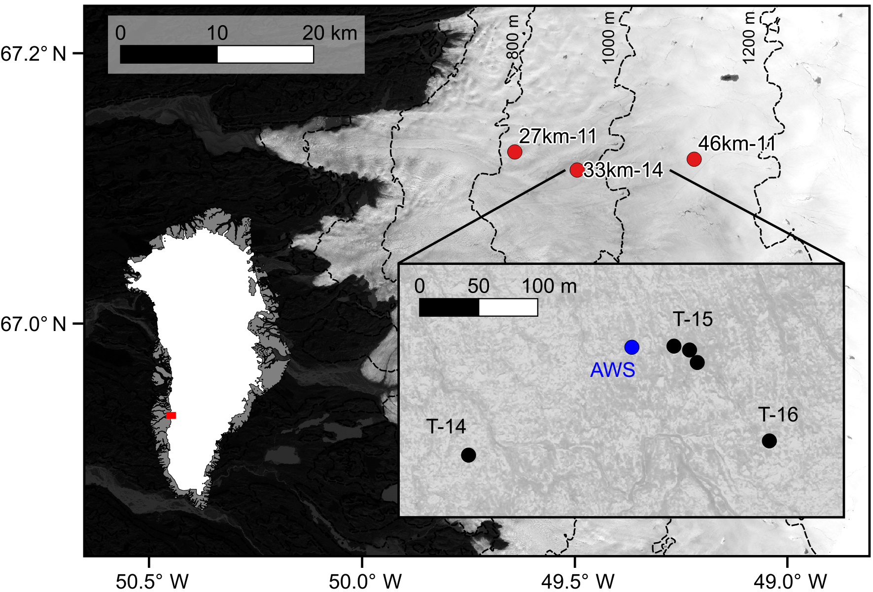
Figure 1A site map from western Greenland with field sites (red) named by their location with respect to the outlet terminus of Isunnguata Sermia and the two-digit year the site was first visited (i.e. 27km-11). The inset shows locations of near-surface temperature strings (black) named by the year they were installed and an automated weather station (blue). Surface elevation contours are shown at 200 m spacing (Howat et al., 2014).
At each field site, boreholes for temperature instrumentation were drilled from the surface to between 10 and 21 m depth using hot-water methods. In total, seven strings of temperature sensors were installed – one at both 27km-11 and 46km-11 in 2011, followed by five at 33km-14 between 2014 and 2016. Strings are named by the year they were installed. Each consists of between 17 and 32 sensors spaced at 0.5–3.0 m along the cable (Table 1). In 2011 and 2014, thermistors were used as temperature sensors. The thermistors have a measurement resolution of 0.02 ∘C and accuracy of about 0.5 ∘C after accounting for drift (Humphrey et al., 2012). In subsequent years, we used a digital temperature sensor (model DS18B20 from Maxim Integrated Products, Inc.). This sensor has a resolution of 0.0625 ∘C and about the same accuracy as the thermistors. To increase accuracy, each sensor was lab calibrated in a 0 ∘C bath and field calibrated with a temperature measurement during freeze-in (borehole water is exactly 0 ∘C). Because each temperature sensor is in a black casing, the measurement error surely increases due to solar heating as sensors move into the rotten cryoconite layer (∼0.2 m depth), and we completely discard any measurement taken after the sensor is exposed at the surface.
Meteorological variables were measured at each field site as well. In this study, we use the near-surface (∼2 m) air temperature (Vaisala HMP60 with a radiation shield), the net radiative heat flux over all wavelengths shorter than 100 µm (Kipp and Zonen NR Lite), and the change in surface elevation measured with a sonic distance sensor (Campbell SR50A). Data from the sonic distance sensor are filtered manually, removing any obvious outliers (more than 0.5 m from the surrounding measurements). The filtered data are then partitioned into two variables, cumulative ablation during the melt season and changes in snow depth during the winter. An automated weather station with all the above instrumentation was mounted on a fixed pole frozen in the ice, with segments being removed from the mounting pole each summer so the instrumentation remains close to the surface and does not extend significantly into the air temperature inversion (Miller et al., 2013). Out of concern for error in our air temperature measurement, we offer a comparison (Fig. S4 in the Supplement) to the nearby weather station monitored by the Programme for Monitoring of the Greenland Ice Sheet (PROMICE) (van As et al., 2012). The measurement frequency for meteorological data varies from 10 min to an hour, but all data are collapsed to a daily mean for input to a heat transfer model.
In addition to ice temperature and meteorological measurements, investigations of the subsurface were completed at 33km-14 with a borehole video camera and a high-frequency ground-penetrating radar survey (see Supplement). These investigations were carried out in pursuit of what we think may have been subsurface fractures that are not expressed at the ice surface (described in Sect. 5.2). With five temperature sensor strings, an automated weather station, and the subsurface investigations, 33km-14 is by far the most thoroughly studied of the three sites. For that reason, measurements from this site serve as the foundation for the model case study presented in Sect. 4.
3.1 Observed ice temperature
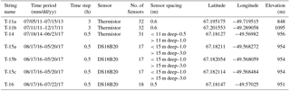
Near-surface ice temperatures were measured through time in seven shallow boreholes at three different field sites (Fig. 2). Although hot-water drilling methods temporarily warm ice near the instrumentation, the ice around these shallow boreholes cools to its original temperature within days to weeks. Measured temperatures are spatially variable between sites. The mean value from the lowermost sensor (analogous to T0) is −3.2 ∘C at 27km-11, −8.6 ∘C at 46km-11, and from −9.7 to −8.1 ∘C at 33km-14. In all cases, measured T0 values are warmer than the mean annual air temperature. Temperature gradients are calculated by fitting a line to the mean temperature of the four lowermost sensors for each string. These gradients are also variable, typically being between −0.15 and 0.0 ∘C m−1 but +0.16 ∘C m−1 at 27km-11 (positive being increasing temperature with depth below the surface). As expected, the direction of the temperature gradients measured here correlate with those measured in the uppermost ∼100 m for full-thickness temperature profiles (Harrington et al., 2015; Hills et al., 2017).
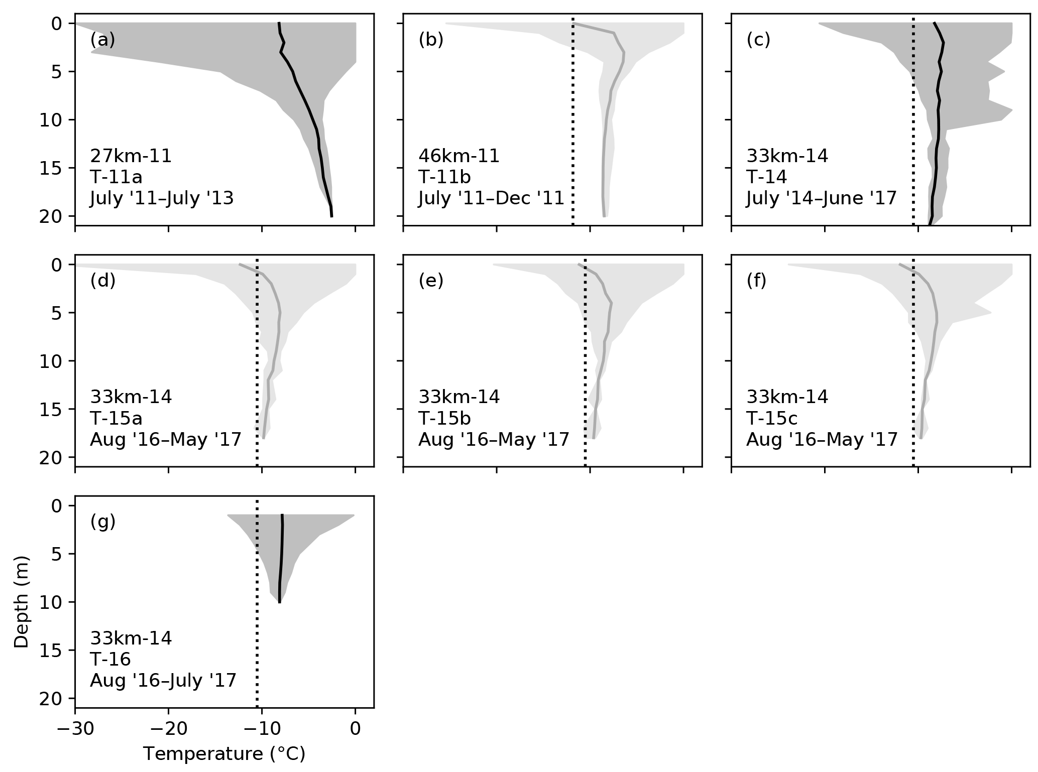
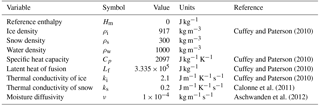
Figure 2Near-surface ice temperature measurements from seven strings: T-11a, T-11b, T-14, T-15a, T-15b, T-15c, and T-16. For each, the shaded region shows the range of measured temperatures over the entire measurement period, and the solid line indicates the mean temperature profile. Depths are plotted with respect to the surface at the time of measurement, so sensor locations move toward the surface as ice melts. Strings with less than 11 months of data are slightly more transparent. For field sites at which the air temperature was measured for at least a full year, a dashed line shows the mean air temperature.
Even the five temperature profiles measured at 33km-14 exhibit some amount of spatial variability. Three temperature strings, T-15a, b, and c, are all similar, having strong negative temperature gradients (approximately −0.14 ∘C m−1) and cold T0 temperatures (−9.6 ∘C). Close to the surface, these three temperature strings are cold compared to the others. However, those strings stopped collecting measurements in May 2017 and did not yield a full year of data. The missing summer period explains the strong positive temperature gradient near the surface for those three strings. T-16 is the shortest string, extending to only 9.5 m depth. This short string exhibits the smallest range in temperatures throughout a season with the coldest surface temperatures not even reaching −15 ∘C. In terms of mean temperature, T-16 is similar to T-14, having a small negative temperature gradient and warm temperatures in comparison to those of T-15a, b, and c. Based on our observations, spatial variability in near-surface ice temperature at 33km-14 is controlled on the scale of hundreds of meters. Proximal observations from the nearby T-15a, b, and c strings are similar to one another, but greater variability is observed when including the more distant strings, T-14 and T-16.
Closer inspection of the measured temperature record through time reveals the transient nature of near-surface ice temperature (Fig. 3). As expected, these data show a strong seasonal oscillation near the surface. During the melt season, the ice surface quickly drops as ice is warmed to the melting point. Just below the surface, the winter cold wave persists for several weeks into the summer season. In string T-14 we observe delayed freeze-in behavior in one sensor (Fig. 3b) and transient heating events during the melt seasons (Fig. 3c, d, e). Similar heating events were observed in string T-16 (Fig. 4) but not in any other. The events range in magnitude, but in one instance ice is warmed from −10 to −2 ∘C in 2 h (Fig. 3c). We can only speculate on the origins of these events and address this below in Sect. 5.2.
Figure 3Three years of ice temperature measurements from the T-14 string. While this string was initially installed to 21 m depth, measurements are plotted with reference to the moving surface, so the sensors move up throughout the time period, revealing a gray mask. Transient features in the data include anomalously slow freeze-in behavior in one sensor (b) as well as heating events throughout the collection time period (c, d, e). The heating events are plotted as a series of temperature profiles with the darker shades being later times and time steps between profiles of 2 h (c), 10 h (d), and 1 h (e).
3.2 Meteorological data
Meteorological data from 33km-14 were observed over 3 years (Supplement Fig. S3). Air temperatures are normally at or above the melting temperature during the summer but fall to below −30 ∘C in winter months. The measured ablation rate is 2–3 m yr−1 and maximum snow accumulation is only up to 0.5 m. Net radiation is less than zero in the winter (net outgoing because thermal emission in the infrared wavelengths dominates over atmospheric inputs) but over 100 W m−2 (daily mean) on some days in the summer.
The mean air temperature over the entire measurement period at 33km-14 (−10.5 ∘C) is cold in comparison to measured ice temperatures at that site (Fig. 2; T-14, T-15a, T-15b, T-15c, and T-16). This warm anomaly between the ice and air temperature is also observed at 27km-11 and 46km-11, where ice is warmer than the measured air temperature and significantly warmer than the reference from a regional climate model (Meierbachtol et al., 2015). Interestingly, we measure almost no winter snowpack at 27km-11 and 46km-11 due to low precipitation and strong winds during the time period over which those data were collected (2011–2013). Our observations are thus in contradiction to the inferences made by Hooke et al. (1983) in Arctic Canada, where the offset between air and ice temperature appeared to be primarily a result of snow insulation.
Overall, the 3 years for which meteorological data were collected are significantly different. The 2014–2015 winter was particularly cold, bringing the mean air temperature of that year more than a degree lower than the other two seasons. Snow accumulation was approximately doubled that winter in comparison to the other two. Also, the summer melt season is longer in 2016 than in 2015. In comparison with past trends from the nearby PROMICE station, KAN_L, the second year is more typical for this area (van As et al., 2012). To model a representative season, data from that second year (July 2015 to July 2016) were chosen as annual input for the model case study.
Our objective is now to investigate how various processes active in Greenland's ablation zone influence T0. In order for model results to achieve fidelity, inputs and parameters need to be representative of actual conditions. We therefore use the meteorological data to constrain the modeling experiments. Our modeling is focused at 33km-14, where we have the most data for constraining the problem.
4.1 Model formulation
The foundation for quantifying impacts of near-surface heat transfer processes is a one-dimensional thermodynamic model. We argue that the processes tested here are close enough to being homogeneous that they can be adequately assessed in one dimension. The one exception is the measured heating events, which are transient and spatially discrete; these are discussed in Sect. 5.2 and are not included in the model analysis. Our model uses measured meteorological variables as the surface boundary condition and simulates ice temperature to 21 m, a depth chosen for consistency with measured data. The ice temperature at the depth of zero annual amplitude, T0, is output from the bottom of the domain for each model experiment and used as a metric to compare net temperature changes between simulations. The model, its boundary conditions, and the experiments are all designed to test heat transfer processes within the ice itself. To maintain focus on ice processes, we ignore any atmospheric effects above the ice surface such as turbulent heat fluxes. The model does not, nor is it meant to, simulate the surface mass balance.
We implement an Eulerian framework, treating the z dimension as depth from a moving surface boundary so that emerging ice moves through the domain and is removed when it melts at z=0. We use a finite element model with a first-order linear element and 0.5 m mesh spacing refined to 2 cm near the surface. For a seamless representation of energy across the water/ice phase boundary, we implement an advection–diffusion enthalpy formulation (i.e. Aschwanden et al., 2012; Brinkerhoff and Johnson, 2013),
Here, ∂ is a partial derivative, t is time, u is the vertical ice velocity with respect to the lowering ice surface, z is depth, H is specific enthalpy, α is thermal diffusivity, ϕ is any added energy source, and ρi is the density of ice. The diffusivity term is enthalpy dependent,
where ki is the thermal conductivity of ice which we assume is constant over the small temperature range in this study (∼25 ∘C), Cp is the specific heat capacity which is again assumed constant, ν is the moisture diffusivity in temperate ice, and Hm is the reference enthalpy at the melting point (all constants are shown in Table 2). Aschwanden et al. (2012) include a thermally diffusive component in temperate ice (i.e. ). However, since we consider only near-surface ice, where pressures (P) are low, this term reduces to zero. Using this formulation, energy moves by a sensible heat flux in cold ice and a latent heat flux in temperate ice. We assume that the latent heat flux, prescribed by temperate ice diffusivity (ν∕ρi) in Eq. 2), is an order of magnitude smaller than the cold ice diffusivity (ki∕ρiCp). We argue that this is representative of the near-surface ice when cold ice is impermeable to meltwater.
The desired model output is ice temperature. It has been argued that temperature is related to enthalpy through a continuous function, where the transition between cold and temperate ice is smooth over some “cold-temperate transition surface” (Lüthi et al., 2002). On the other hand, we argue that cold ice is impermeable to water except in open fractures (which we do not include in these simulations), so we use a stepwise transition,
Additional enthalpy above the reference increases the water content in ice,
where Lf is the latent heat of fusion. If enough energy is added to ice that its temperature would exceed the melting point, excess energy goes to melting. In our case study, we limit the water content based on field observations of water accumulation in the layer of rotten ice and cryoconite holes. This rotten cryoconite layer extends to approximately 20 cm depth and as an upper limit accumulates a maximum 50 % liquid water. Therefore, we limit the water content in the rotten cryoconite layer,
with any excess melt immediately leaving the model domain as surface runoff.
The two boundary conditions are (1) fixed to the air temperature at the surface,
and (2) free at the bottom of the domain,
Both boundary conditions are with no liquid water content, ω=0. The surface boundary condition is updated at each time step to match the measured air temperature. The bottom boundary condition is fixed in time. This bottom boundary condition is also changed for some model experiments to test the influence of a temperature gradient at the bottom of the domain (Sect. 4.2.4).
4.2 Experiments
Four separate model experiments are run, each with a new process incorporated into the physics and each guided by observational data. All simulations use the enthalpy formulation above rather than temperature in order to track the internal energy of the ice–water mixtures that are prevalent in the ablation zone. The results from each experiment are referenced to an initial control run, which is simple thermal diffusion of the measured air temperature in the absence of any additional heat transfer processes. Meteorological data are input where needed for an associated process in the model. These data are clipped to 1 full year and input at the surface boundary in an annual cycle. The model is run with a 1-day time step until ice temperature at the bottom of the domain converges to a steady temperature. A description of each of the model experiments follows below. These experiments build on one another, so each new experiment incorporates the physics of all previously discussed processes.
4.2.1 Ablation
The first experiment simulates motion of the ablating surface. While the control run is performed with no advective transport (i.e. u=0), in this experiment we incorporate advection by setting the vertical velocity equal to measurements of the changing surface elevation through time. When ice melts, the ice surface location drops. Because the vertical coordinate, z, in the model domain is treated as a distance from the moving surface, ablation brings simulated ice closer to the surface boundary. Hence, the simulated ice velocity, u, is assigned to the ablation rate (except in the opposite direction, ice moves upward) for this first model experiment. The ablation rate is calculated as a forward difference of the measured surface lowering.
4.2.2 Snow insulation
The second experiment incorporates measured snow accumulation, which thermally insulates the ice from the air. The upper boundary condition is now assigned to the snow surface, the location of which changes in time. Diffusion through the snowpack is then simulated as an extension of the ice domain but with different physical properties. The thermal conductivity of snow (Calonne et al., 2011),
is dependent on snow density, ρs, for which we use a constant value, 300 kg m−3. We treat the specific heat capacity of snow to be the same as ice (Yen, 1981).
4.2.3 Radiative energy
The third model experiment incorporates an energy source from the net radiation measured at the surface. Energy from radiation is absorbed in the ice and is transferred to thermal energy and to ice melting (van den Broeke et al., 2008). We assume that all this radiative energy is absorbed in the uppermost 20 cm, the rotten cryoconite layer, and if snow is present the melt production immediately drains to that cryoconite layer. When the net radiation is negative (wintertime), we assume that it is controlling the air temperature, so it is already accommodated in our simulation; thus, the radiative energy input is ignored in the negative case. This radiative source term is incorporated into Eq. (1) at each time step, , where Q is the measured radiative flux at the surface in W m−2. All constants for the rotten cryoconite layer are the same as that for ice.
While some models treat the absorption of radiation in snow and ice more explicitly with a spectrally dependent Beer–Lambert law (Brandt and Warren, 1993), we argue that it is reasonable to assume all wavelengths are absorbed near the surface over the length scales that we consider. The only documented value that we know of for an absorption coefficient in the cryoconite layer is 28 m−1 (Lliboutry, 1965), which is close to that of snow (Perovich, 2007). If the properties are truly similar to that of snow, about 90 % of the energy is absorbed in the uppermost 20 cm (Warren, 1982). Moreover, we argue that this is precisely the reason that the cryoconite layer only extends to a limited depth; it is a result of where radiative energy causes melting.
4.2.4 Subsurface temperature gradient
Finally, in the fourth model experiment we change the boundary condition at the bottom of the domain. The free boundary is changed to a Neumann boundary with a gradient of −0.05 ∘C m−1, a value that approximately matches the measured gradient at 33km-14. Importantly, this simulated gradient is in the same direction, although with a larger magnitude, as the upper ∼100 m of ice in our measurements of deep temperature profiles (Hills et al., 2017). In this case, the advective energy flux is upward, but the temperature gradient is negative, bringing colder ice to the surface. In addition, two limiting cases were tested, with gradients of ±0.15 ∘C m−1. This is the approximate range in the measured gradients (Fig. 2).
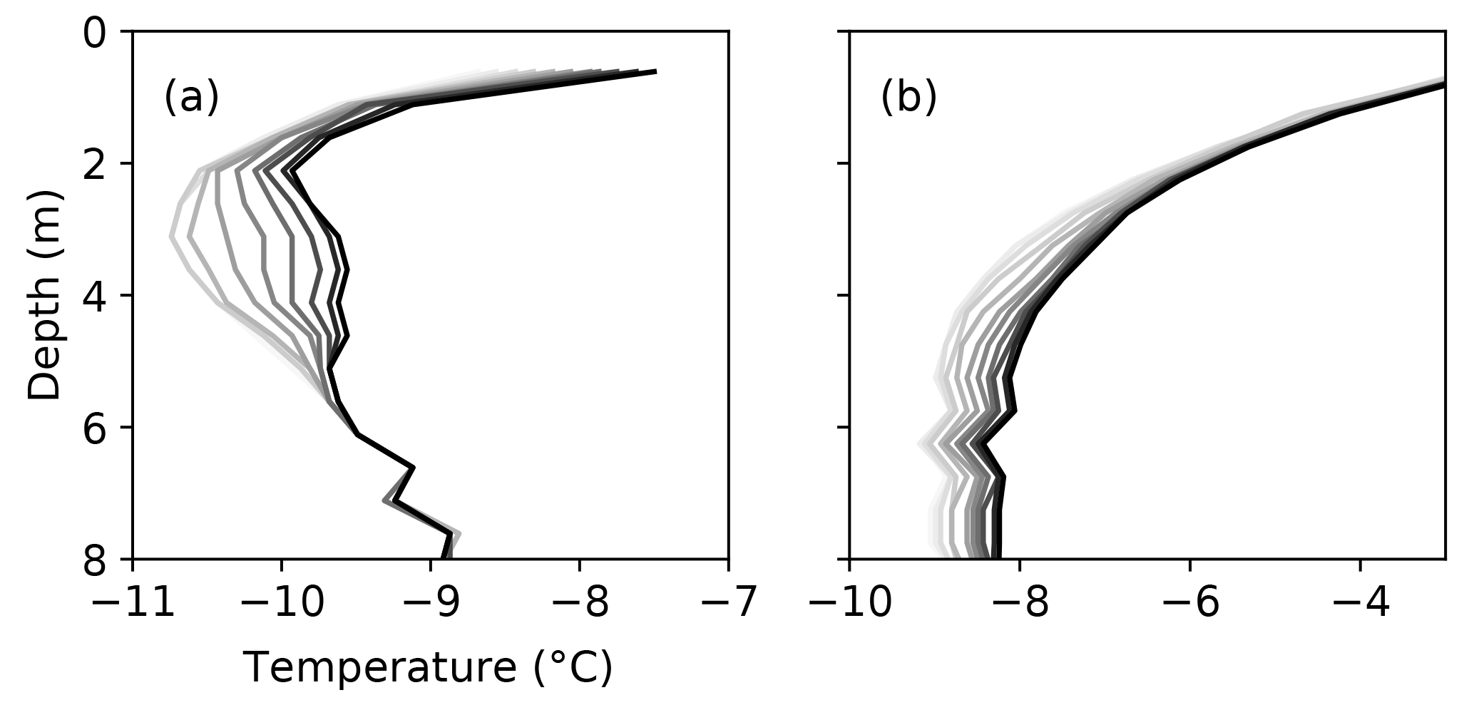
Figure 4Heating events from temperature string T-16. Profiles are plotted as in Fig. 3c, d, and e. The time steps between profiles are 2 h (a) and 4 h (b).
4.3 Model results
The control model run of simple thermal diffusion predicts that ice temperature converges to approximately the mean annual air temperature of the study year (−9.9 ∘C) by about 15 m below the ice surface. This result is in agreement with the analytical solution (Carslaw and Jaeger, 1959) but is slightly different from the mean air temperature (−9.6 ∘C) because the air can exceed the melting temperature in the summer, while the ice cannot. Other atmospheric effects such as turbulent heat fluxes and the thermal inversion could also cause a difference between measured air temperature and ice surface temperature, but these are not considered here. For each model treatment, 1–4, the incorporation of an additional physical process changes the ice temperature. Differences between model runs are compared using T0 at 21 m. Again, the model experiments are progressive, so each new experiment includes the processes from all previous experiments. Key results from each experiment are as follows (Fig. 5):
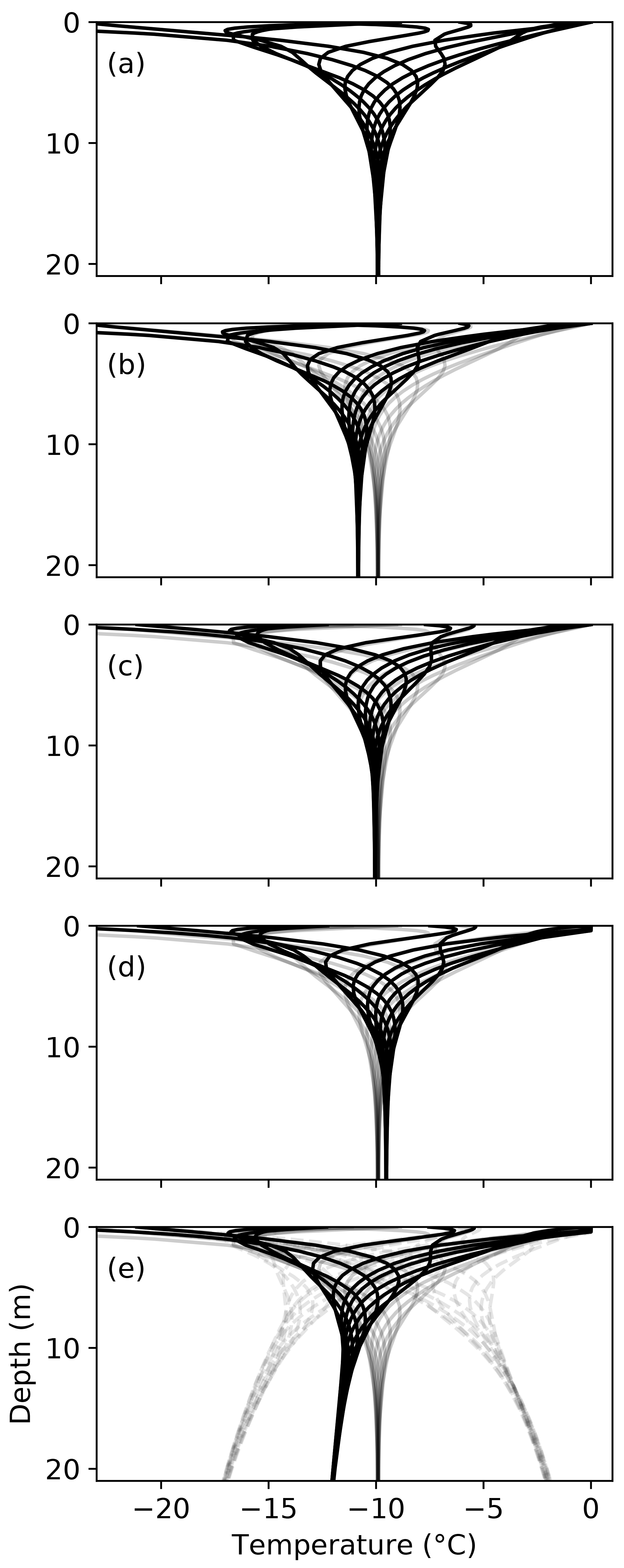
Figure 5Model results for five separate simulations. In each case, twelve simulated temperature profiles are shown throughout the year-long period, and control results (from a) are displayed for comparison (gray). Differences between the simulations are analyzed quantitatively using T0, the convergent temperature at 21 m. Processes are, from top to bottom, (a) control simulation of pure diffusion, (b) ablation, (c) snow insulation, (d) radiative energy input, and finally (e) subsurface temperature gradient. The two limiting cases for the subsurface temperature gradient are plotted with dashed gray lines (e).
-
Diffusion alone results in ∘C, whereas observed temperatures range from −9.7 to −8.1 ∘C at 33km-14.
-
Because the ablation rate is strongest in the summer, the effect of incorporating ablation is to counteract the diffusion of warm summer air temperatures. The result is a net cooling of T0 from experiment (1) by −0.92 ∘C.
-
Snow on the ice surface insulates the ice from the air temperature. In the winter, snow insulation keeps the ice warmer than the cold air, but with warm air temperatures in the spring it has the opposite effect. Because snow quickly melts in the springtime, the net effect of snow insulation is substantially more warming than cooling. T0 for this experiment is +0.78 ∘C warmer than the previous one.
-
Radiative energy input mainly controls melting (van den Broeke et al., 2008), but incorporating this process does warm T0 by +0.52 ∘C.
-
Imposing a −0.05 ∘C m−1 temperature gradient at the bottom of the model domain, consistent with observations, dramatically changes T0 by −2.5 ∘C.
Both ablation and the subsurface temperature gradient have a cooling effect on near-surface ice temperature. On the other hand, snow and radiative energy input have a warming effect. For this case study, the first three processes together result in almost no net change, so that the modeled T0 is close to the observed mean air temperature (Fig. 5d). However, inclusion of the subsurface temperature gradient has a strong cooling effect on the simulated temperatures, bringing T0 far from the mean measured air temperature. The limiting cases show that this bottom boundary condition strongly controls the near-surface temperature, with a range in the resulting T0 values from −17.0 to −2.0 ∘C. In summary, measured ice temperatures are consistently warmer than both the measured air temperature and simulated ice temperature (Fig. 6), except in the case of a positive subsurface gradient, which is discussed below.
Figure 6A comparison of model output (gray) and data from 33km-14, including mean ice temperatures (red) and mean annual air temperatures for three seasons (black dashed). The observed ice temperatures are plotted the same as in Fig. 2. Note that three of the temperature strings collected only ∼9 months of data (transparent red). Mean temperatures from those three strings are cold near the surface because they collected more measurements in wintertime than summertime.
Our observations show that measurements of near-surface ice in the ablation zone of western Greenland are significantly warmer than would be predicted by diffusive heat exchange with the atmosphere. This is in agreement with past observations collected in other ablation zones (Hooke et al., 1983). With four experiments in a numerical model that progressively incorporate more physical complexity, we are unable to precisely match independent model output to observations. Our measurement and model output point toward a disconnect between air and ice temperatures in the GrIS ablation zone, with ice temperatures being consistently warmer than the air.
5.1 Ablation–diffusion
The strongest result from our model case study was a drop in T0 by −2.5 ∘C associated with the imposed subsurface temperature gradient. While it was important to test this scenario for one case, the temperature gradient we used was representative but somewhat arbitrary. In reality, the observed temperature gradients are widely variable from one site to another and even within one site (Fig. 2). Interestingly, full ice thickness temperature profiles show similar temperature gradients, both positive and negative (Harrington et al., 2015; Hills et al., 2017). Hence, the limiting cases were added to show simulation results over the range of measured gradients from our temperature strings. The resulting T0 values span a range of 19 ∘C.
The majority of the subsurface temperature gradients that we measure are negative, and theoretically the gradient should be negative. Consider that fast horizontal velocities (∼100 m yr−1) advect cold ice from the divide to the ablation zone, and the air temperature lapse rate couples with the relatively steep surface gradients so that the surface warms rapidly toward the terminus. These conditions lead to a vertical temperature gradient below the ice surface that is negative (Hooke, 2005; pp. 131–135), as in our model example. The one exception is in the case of deep latent heating in a crevasse field (Harrington et al., 2015; sites S3 and S4), where the deep ice temperature is warmer than the mean air temperature rather than colder.
Overall, our results demonstrate that the effect of the subsurface temperature gradient is coupled to that of surface lowering. With respect to the surface, the temperature gradient below is advected upward as ice melts. There is competition between surface lowering and diffusion of atmospheric energy into the ice: as near-surface ice gets warmer, it can be removed quickly and a new boundary is set. Therefore, our conceptualization of temperature in the near-surface ice of the ablation zone should not be a seasonally oscillating upper boundary with purely diffusive heat transfer (Carslaw and Jaeger, 1959), but one with advection and diffusion (Logan and Zlotnik, 1995; Paterson, 1972). This conceptualization is unique to the ablation zone because of the rapid rate of surface lowering, whereas a diffusive model for near-surface heat transfer is much more appropriate in the accumulation zone.
The disconnect between air and ice temperature implies that the near-surface active layer in the ablation zone is shallow (i.e. less than 15 m) and could be skewed toward the subsurface temperature gradient. Therefore, the surface boundary condition has weak influence on diffusion for ice well below the surface. This is in contrast to the accumulation zone where new snow is advected downward, so the surface temperature quickly influences that at depth. Under these conditions, it is no surprise that we see spatial variability in near-surface ice temperature even within one field site. That variability is simply an expression of the deeper ice temperature variations, which are hypothesized to exist from variations in vertical advection (Hills et al., 2017), and do not have time to completely diffuse away before they are exposed at the surface.
5.2 Subsurface refreezing
We observe heating events in two temperature strings, the largest case being 8 ∘C in 2 h between 3 and 8 m below the ice surface (Fig. 3c). These events are transient, they are spatially discrete, and they are generated at depth. All of these factors are most easily explained by the refreezing of liquid water in cold ice. Similar refreezing events have been observed in firn (Humphrey et al., 2012), where they are not only important for ice temperature but could also imply a large storage reservoir for surface meltwater (Harper et al., 2012). However, unlike firn, solid ice is impermeable to water unless fractures are present (Fountain et al., 2005). Two persistently warm features are also observed between 5 and 10 m depth into the winters of 2015 and 2017 (Fig. 3a). We interpret these as a nearby latent heat source, either with running or ponded water that does not freeze for an extended time.
In Greenland's ablation zone, prior work has demonstrated the importance of large-scale latent heating in open crevasses (Phillips et al., 2013; Poinar et al., 2016). Additionally, water-filled cavities have been observed in cold, near-surface ice on mountain glaciers (Jarvis and Clarke, 1974; Paterson and Savage, 1970). In our case, however, an explanation for refreezing water is not obvious. While the field site has occasional millimeter-aperture “hairline” cracks, there are no visible open crevasses at the surface for routing water to depth. As far as we know, this work is the first to report evidence of short-term transient latent-heating events in cold ice that is not obviously linked to open surface fractures.
While the hairline fractures could perhaps move some water, to permit much water to move meters through cold ice they would need to be large enough that water moves quickly and does not instantaneously refreeze. For example, a 1 mm wide crack in ice that is −10 ∘C freezes shut in about 45 s (Alley et al., 2005; Eq. 8). That amount of time could be long enough for small volumes of water to move 5–10 m below the surface but would require a hydropotential gradient to drive water flow. Thus, top-down hairline crevassing does not seem a plausible explanation for the events we observe.
Importantly, several independent field observations in this area, including hole drainage of water during hot-water drilling, ground-penetrating radar reflections, and borehole video observations, all point to the existence of subsurface air-filled and open fractures with apertures of up to a few centimeters (see Supplement). That they are open at depth, but are narrow or nonexistent at the surface, could be linked to the colder ice at depth and its stiffer rheology. Nath and Vaughan (2003) observed similar subsurface fractures in firn, although in their case density controls the stiffness rather than temperature. On rare occasions, we argue that the aperture of the fractures open wider to the surface, where there is copious water stored in the cryoconite layer (Cooper et al., 2018) that can drain and refreeze at depth. While the events seem to happen in the springtime and it would be tempting to assert that fracture opening coincides with speedup, our measurements of surface velocity at these sites show that this is not always the case. This may be due to that fact that the spring speedup coincides with early melt rather than peak melt and copious water in the cryoconite layer.
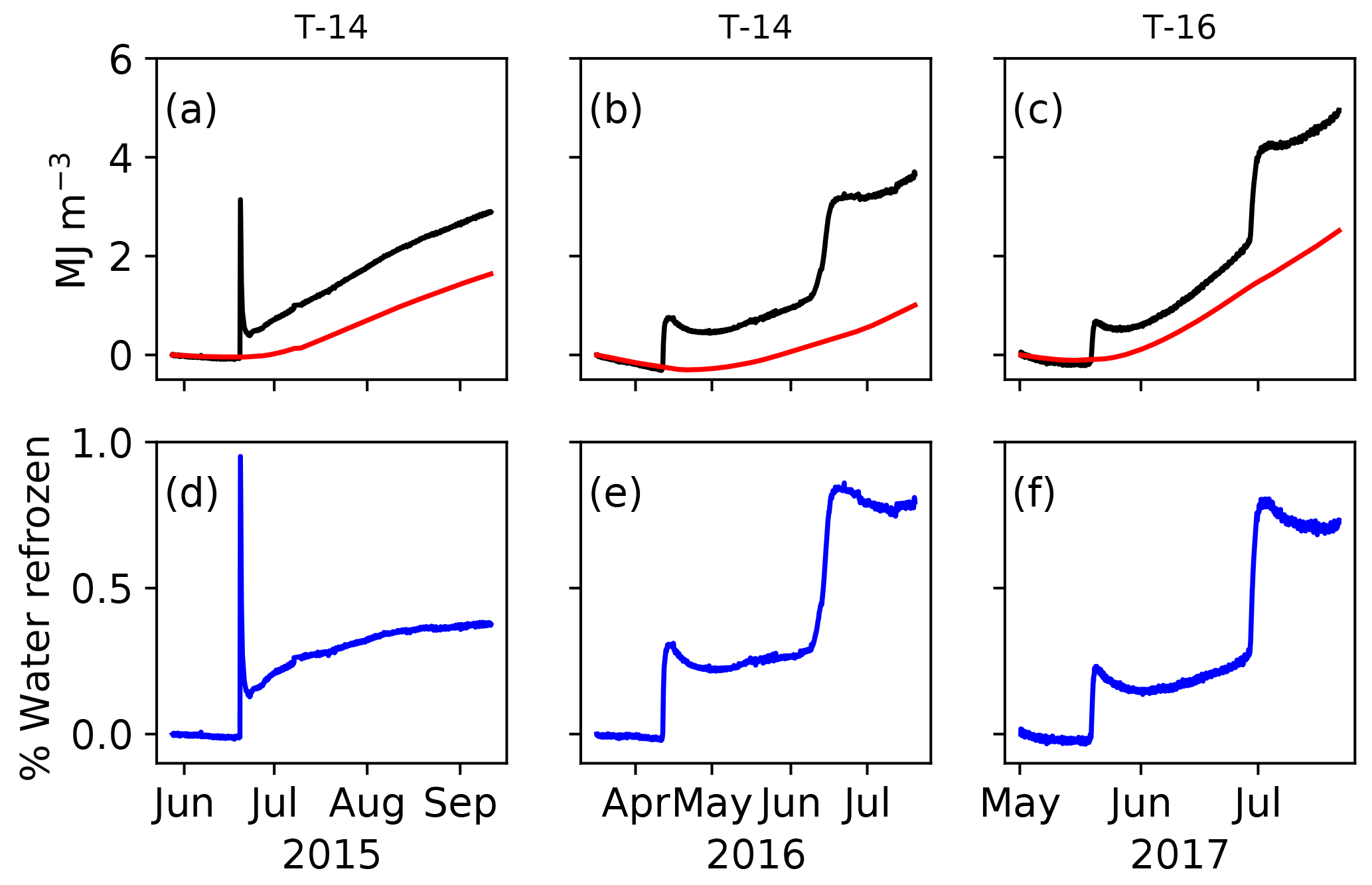
Figure 7Energy source for the observed heating events. (a–c) Observed energy density through time for the differenced temperature profile calculated with Eq. (9) (black) and conductive energy density through time calculated with Eq. (10) (red). (d–f) Percentage by volume water refrozen for the associated source in (a–c). This value is proportional to the difference between the black and red lines above. The temperature string from which measurements were taken is labeled at the top.
Latent heating in the form of these subsurface refreezing events is an obvious candidate for a source for the “extra” heat we observe in our temperature strings relative to simulations. Our data show that refreezing in subsurface fractures has the potential to warm ice substantially over short periods of time, and apparently this can occur in places where open crevasses are not readily observed at the surface. Furthermore, the difference between measured and modeled temperatures (up to 3 ∘C) is the equivalent of only ∼1.7 % water by volume. Our simplified one-dimensional model would not be well suited to assess the influence of these latent heating events. Instead, we provide a simple calculation for energy input from the events by differencing the temperature profiles in time and integrating for total energy density (Fig. 7a–c),
where Δz is the total depth of the profile, and ΔT is the differenced temperature profile. Only sensors that are below the ice surface for the entire time period are considered. To calculate the total water content refrozen in the associated event, we remove the conductive energy fluxes from the total energy density calculated above. We do this by calculating the temperature gradients at the top and bottom of the measured temperature profile at each time step as in Cox et al. (2015):
The resulting energy sources are then converted to a volume fraction of water by
where ρw is the density of water. Results show that each year some fractions of a percentage of water are refrozen (Fig. 7). Through several seasons that amount of refreezing could easily add up to the ∼3 ∘C anomaly that we observe.
Unfortunately, without a more thorough investigation, we do not have enough evidence to show that these refreezing events are more than a local anomaly. Of our seven near-surface temperature strings, only T-14 and T-16 demonstrated refreezing events, so we are not confident that they are temporally or spatially ubiquitous.
The only other logical mechanism for the warm offset between measurements and model results would be warming from below through a positive subsurface temperature gradient. While it is tempting to associate deep warm ice with residual heat from the exceptionally hot summers of 2010 and 2012 (Tedesco et al., 2013), this scenario is unlikely because the ablation rates are so high that any ice warmed during those years has likely already melted. Deeper latent heating from an upstream crevasse field is a more plausible alternative; however, full-depth temperature profiles from 33km-14 do not show deeper ice to be anomalously warmed except in one localized case (Hills et al., 2017).
We observe the temperature of ice at the depth of zero annual amplitude, T0, in Greenland's ablation zone to be markedly warmer than the mean annual air temperature. These findings contradict predictions from purely diffusive heat transport but are not surprising considering the processes which impact heat transfer in the ice of the ablation zone. High ablation rates in this area indicate that ice temperatures below 15 m reflect the temperature of deep ice that is emerging to the surface, confirming that the ice does not have time to equilibrate with the atmosphere. In other words, ice flow brings cold ice to the surface at a faster rate than heat from the atmosphere can diffuse into the ablating surface. The coupling between rapid ablation and the spatial variability in deep ice temperature implies there will always be a disconnect between air and ice temperatures. Additionally, we observe refreezing events below 5–10 m of cold ice. Meltwater is likely moving to that depth through subsurface fractures that are not obviously visible at the surface.
In analyzing a series of processes that control near-surface ice temperature, we find that some lead to colder ice and others to warmer ice, but most are strong enough to dramatically alter the ice temperature from the purely diffusive case. With rapid ablation, a spatially variable temperature field, and subsurface refreezing events, T0 in the ablation zone should not be expected to match the air temperature. That our measurements are consistently warmer could simply be due to the limited number of observations we have, but latent heat additions are clearly measured and could be common in near-surface ice of the western Greenland ablation zone.
All temperature measurements are available at https://doi.org/10.18739/A2G44HQ01 (Hills, 2018).
The supplement related to this article is available online at: https://doi.org/10.5194/tc-12-3215-2018-supplement.
BHH, JVJ, NFH, and PJW designed and built instrumentation for temperature measurements. BHH wrote the numerical model with JTH and TWM contributing to model experiment design. BHH led the writing with significant input from all co-authors.
The authors declare that they have no conflict of interest.
This work was funded by the National Science Foundation (Office of Polar
Programs-Arctic Natural Sciences grant no. 1203451 and no. 0909495). We thank
the editor, Tobias Sauter, and two anonymous reviewers for their comments,
which greatly improved the original
manuscript. We also thank Stephen Warren for valuable discussions.
Edited by: Tobias Sauter
Reviewed by: two anonymous referees
Alley, R. B., Dupont, T. K., Parizek, B. R., and Anandakrishnan, S.: Access of surface meltwater to beds of sub-freezing glaciers: Preliminary insights, Ann. Glaciol., 40, 8–14, https://doi.org/10.3189/172756405781813483, 2005.
Aschwanden, A., Bueler, E., Khroulev, C., and Blatter, H.: An enthalpy formulation for glaciers and ice sheets, J. Glaciol., 58, 441–457, https://doi.org/10.3189/2012JoG11J088, 2012.
Brandt, R. and Warren, S.: Solar-heating rates and temperature profiles in Antarctica snow and ice, J. Glaciol., 39, 99–110, 1993.
Brinkerhoff, D. J. and Johnson, J. V.: Data assimilation and prognostic whole ice sheet modelling with the variationally derived, higher order, open source, and fully parallel ice sheet model VarGlaS, The Cryosphere, 7, 1161–1184, https://doi.org/10.5194/tc-7-1161-2013, 2013.
Calonne, N., Flin, F., Morin, S., Lesaffre, B., Du Roscoat, S. R., and Geindreau, C.: Numerical and experimental investigations of the effective thermal conductivity of snow, Geophys. Res. Lett., 38, 1–6, https://doi.org/10.1029/2011GL049234, 2011.
Carslaw, H. S. and Jaeger, J. C.: Conduction of Heat in Solids, 2nd Edn., London: Oxford University Press, 1959.
Cooper, M. G., Smith, L. C., Rennermalm, A. K., Miège, C., Pitcher, L. H., Ryan, J. C., Yang, K., and Cooley, S. W.: Meltwater storage in low-density near-surface bare ice in the Greenland ice sheet ablation zone, The Cryosphere, 12, 955–970, https://doi.org/10.5194/tc-12-955-2018, 2018.
Cox, C., Humphrey, N., and Harper, J.: Quantifying meltwater refreezing along a transect of sites on the Greenland ice sheet, The Cryosphere, 9, 691–701, https://doi.org/10.5194/tc-9-691-2015, 2015.
Cuffey, K. and Paterson, W. S. B.: The Physics of Glaciers, 4th Edn., Oxford, UK, Butterworth-Heinemann, 2010.
Fountain, A. G., Jacobel, R. W., Schlichting, R., and Jansson, P.: Fractures as the main pathways of water flow in temperate glaciers, Nature, 433, 618–621, https://doi.org/10.1038/nature03296, 2005.
Harper, J. T., Humphrey, N. F., Pfeffer, W. T., Brown, J., and Fettweis, X.: Greenland ice-sheet contribution to sea-level rise buffered by meltwater storage in firn, Nature, 491, 240–243, https://doi.org/10.1038/nature11566, 2012.
Harrington, J. A., Humphrey, N. F., and Harper, J. T.: Temperature distribution and thermal anomalies along a flowline of the Greenland Ice Sheet, Ann. Glaciol., 56, 98–104, https://doi.org/10.3189/2015AoG70A945, 2015.
Hills, B.: Near-surface ice temperature measurements from Western Greenland, 2011–2017, urn:node:ARCTIC, https://doi.org/10.18739/A2G44HQ01, 2018.
Hills, B. H., Harper, J. T., Humphrey, N. F., and Meierbachtol, T. W.: Measured horizontal temperature gradients constrain heat transfer mechanisms in Greenland ice, Geophys. Res. Lett., 44, 1–8, https://doi.org/10.1002/2017GL074917, 2017.
Hooke, R. L.: Near-surface temperatures in the superimposed ice zone and lower part of the soaked zone of polar ice sheets, J. Glaciol., 16, 302–304, 1976.
Hooke, R. L.: Principles of Glacier Mechanics, 2nd Edn., Cambridge University Press, 2005.
Hooke, R. L., Gould, J. E., and Brzozowski, J.: Near-surface temperatures near and below the equilibrium line on polar and subpolar glaciers, Z. Gletscherkd. Glazialgeol., 19, 1–25, 1983.
Howat, I. M., Negrete, A., and Smith, B. E.: The Greenland Ice Mapping Project (GIMP) land classification and surface elevation data sets, The Cryosphere, 8, 1509–1518, https://doi.org/10.5194/tc-8-1509-2014, 2014.
Humphrey, N. F., Harper, J. T., and Pfeffer, W. T.: Thermal tracking of meltwater retention in Greenland's accumulation area, J. Geophys. Res., 117, 1–11, https://doi.org/10.1029/2011JF002083, 2012.
Jarvis, G. T. and Clarke, G. K. C.: Thermal effects of crevassing on Steele Glacier, Yukon Territory, Canada, J. Glaciol., 13, 243–254, 1974.
Liston, G. E., Winther, J.-G., Bruland, O., Elvehoy, H., and Sand, K.: Below-surface ice melt on the coastal Antarctic ice sheet, J. Glaciol., 45, 273–285, 1999.
Lliboutry, L. A.: Traité de Glaciologie, Vol. 2, Masson, Paris, 1965.
Loewe, F.: Screen temperatures and 10 m temperatures, J. Glaciol., 9, 263–268, 1970.
Logan, J. D. and Zlotnik, V.: The convection-diffusion equation with periodic boundary conditions, Appl. Math. Lett., 8, 55–61, https://doi.org/10.1016/0893-9659(95)00030-T, 1995.
Lüthi, M., Funk, M., Iken, A., Gogineni, S., and Truffer, M.: Mechanisms of fast flow in Jakobshavn Isbræ, West Greenland: Part III, measurements of ice deformation, temperature and cross-borehole conductivity in boreholes to the bedrock, J. Glaciol., 48, 369–385, 2002.
Lüthi, M. P., Ryser, C., Andrews, L. C., Catania, G. A., Funk, M., Hawley, R. L., Hoffman, M. J., and Neumann, T. A.: Heat sources within the Greenland Ice Sheet: dissipation, temperate paleo-firn and cryo-hydrologic warming, The Cryosphere, 9, 245–253, https://doi.org/10.5194/tc-9-245-2015, 2015.
Meierbachtol, T. W., Harper, J. T., Johnson, J. V., Humphrey, N. F., and Brinkerhoff, D. J.: Thermal boundary conditions on western Greenland: Observational constraints and impacts on the modeled thermomechanical state, J. Geophys. Res.-Earth, 120, 623–636, https://doi.org/10.1002/2014JF003375, 2015.
Miller, N. B., Turner, D. D., Bennartz, R., Shupe, M. D., Kulie, M. S., Cadeddu, M. P., and Walden, V. P.: Surface-based inversions above central Greenland, J. Geophys. Res.-Atmos., 118, 495–506, https://doi.org/10.1029/2012JD018867, 2013.
Mock, S. J. and Weeks, W. F.: The distribution of 10 meter snow temperatures on the Greenland Ice Sheet, J. Glaciol., 6, 23–41, 1966.
Müller, F.: On the thermal regime of a high-arctic valley glacier, J. Glaciol., 16, 119–133, 1976.
Nath, P. C. and Vaughan, D. G.: Subsurface crevasse formation in glaciers and ice sheets, J. Geophys. Res., 108, 1–12, https://doi.org/10.1029/2001JB000453, 2003.
Paterson, W. S. B.: Temperature distribution in the upper layers of the ablation area of Athabasca Glacier, Alberta, Canada, J. Glaciol., 11, 31–41, 1972.
Paterson, W. S. B. and Savage, J. C.: Excess pressure observed in a water-filled cavity in Athabasca Glacier, Canada, J. Glaciol., 9, 103–107, 1970.
Perovich, D. K.: Light reflection and transmission by a temperate snow cover, J. Glaciol., 53, 201–210, https://doi.org/10.3189/172756507782202919, 2007.
Phillips, T., Rajaram, H., and Steffen, K.: Cryo-hydrologic warming: A potential mechanism for rapid thermal response of ice sheets, Geophys. Res. Lett., 37, 1–5, https://doi.org/10.1029/2010GL044397, 2010.
Phillips, T., Rajaram, H., Colgan, W., Steffen, K., and Abdalati, W.: Evaluation of cryo-hydrologic warming as an explanation for increased ice velocities in the wet snow zone, Sermeq Avannarleq, West Greenland, J. Geophys. Res.-Earth, 118, 1241–1256, https://doi.org/10.1002/jgrf.20079, 2013.
Poinar, K., Joughin, I., Lenaerts, J. T. M., and van den Broeke, M. R.: Englacial latent-heat transfer has limited influence on seaward ice flux in western Greenland, J. Glaciol., 63, 1–16, https://doi.org/10.1017/jog.2016.103, 2016.
Tedesco, M., Fettweis, X., Mote, T., Wahr, J., Alexander, P., Box, J. E., and Wouters, B.: Evidence and analysis of 2012 Greenland records from spaceborne observations, a regional climate model and reanalysis data, The Cryosphere, 7, 615–630, https://doi.org/10.5194/tc-7-615-2013, 2013.
van As, D., Hubbard, A. L., Hasholt, B., Mikkelsen, A. B., van den Broeke, M. R., and Fausto, R. S.: Large surface meltwater discharge from the Kangerlussuaq sector of the Greenland ice sheet during the record-warm year 2010 explained by detailed energy balance observations, The Cryosphere, 6, 199–209, https://doi.org/10.5194/tc-6-199-2012, 2012.
van den Broeke, M., Smeets, P., Ettema, J., van der Veen, C., van de Wal, R., and Oerlemans, J.: Partitioning of melt energy and meltwater fluxes in the ablation zone of the west Greenland ice sheet, The Cryosphere, 2, 179–189, https://doi.org/10.5194/tc-2-179-2008, 2008.
van de Wal, R. S. W., Boot, W., Smeets, C. J. P. P., Snellen, H., van den Broeke, M. R., and Oerlemans, J.: Twenty-one years of mass balance observations along the K-transect, West Greenland, Earth Syst. Sci. Data, 4, 31–35, https://doi.org/10.5194/essd-4-31-2012, 2012.
van Everdingen, R. O.: Multi-language glossary of permafrost and related ground-ice terms, Calgary, Alberta, CA, International Permafrost Association, 1998.
Warren, S. G.: Optical properties of snow, Rev. Geophys., 20, 67–89, https://doi.org/10.1029/RG020i001p00067, 1982.
Wientjes, I. G. M. and Oerlemans, J.: An explanation for the dark region in the western melt zone of the Greenland ice sheet, The Cryosphere, 4, 261–268, https://doi.org/10.5194/tc-4-261-2010, 2010.
Yen, Y. C.: Review of thermal properties of snow, ice, and sea ice, CRREL Report 81-10, 1981.