the Creative Commons Attribution 4.0 License.
the Creative Commons Attribution 4.0 License.
 | 09 Oct 2018
Grounding-line flux formula applied as a flux condition in numerical simulations fails for buttressed Antarctic ice streams
Ronja Reese
Ricarda Winkelmann
G. Hilmar Gudmundsson
Currently, several large-scale ice-flow models impose a condition on ice flux across grounding lines using an analytically motivated parameterisation of grounding-line flux. It has been suggested that employing this analytical expression alleviates the need for highly resolved computational domains around grounding lines of marine ice sheets. While the analytical flux formula is expected to be accurate in an unbuttressed flow-line setting, its validity has hitherto not been assessed for complex and realistic geometries such as those of the Antarctic Ice Sheet. Here the accuracy of this analytical flux formula is tested against an optimised ice flow model that uses a highly resolved computational mesh around the Antarctic grounding lines. We find that when applied to the Antarctic Ice Sheet the analytical expression provides inaccurate estimates of ice fluxes for almost all grounding lines. Furthermore, in many instances direct application of the analytical formula gives rise to unphysical complex-valued ice fluxes. We conclude that grounding lines of the Antarctic Ice Sheet are, in general, too highly buttressed for the analytical parameterisation to be of practical value for the calculation of grounding-line fluxes.
- Article
(6748 KB) -
Supplement
(11159 KB) - BibTeX
- EndNote


Estimating the future impact of the Antarctic Ice Sheet (AIS) on global sea levels invariably involves calculating changes in ice fluxes across grounding lines, as well as determining the migration of the grounding lines themselves. Accurately describing grounding-line dynamics can therefore be considered an essential prerequisite for any numerical ice-flow simulation of marine ice sheets such as the AIS. Accordingly, over the last decades, considerable efforts have focused on ensuring that large-scale ice-flow models are capable of correctly capturing the dynamical behaviour of grounding lines (Feldmann et al., 2014; Gagliardini et al., 2016; Gladstone et al., 2010; Goldberg et al., 2009; Pattyn et al., 2017; Seroussi et al., 2014). As part of these efforts, several model intercomparison experiments have been conducted to assess different approaches within the ice-sheet modelling community regarding the numerical modelling of marine-type ice sheets (Asay-Davis et al., 2016; Drouet et al., 2013; Pattyn et al., 2012, 2013). Although it is still a subject of active research, one of the outcomes of these intercomparison experiments has been to stress the need for a sufficiently fine resolution of the computational domain around grounding lines. Within the context of the shallow ice-stream computational models – a commonly used flow approximation for describing the flow of ice streams and ice shelves (MacAyeal, 1989; Morland, 1987) – it has, for example, been suggested that for many applications a horizontal resolution of around 1 km or less is suitable (Cornford et al., 2016; Gladstone et al., 2012; Pattyn et al., 2012). However, for large-scale ice flow models using uniform grids, employing such a high resolution globally for large ice sheets such as the AIS can be computationally prohibitively expensive. As a way of resolving this issue, and to allow for an accurate description of grounding-line dynamics without resorting to high spatial resolution, in a number of numerical modelling studies a “flux condition” is imposed at the grounding line, whereby the grounding-line flux is prescribed using an analytical expression (DeConto and Pollard, 2016; Docquier et al., 2011; Pattyn, 2017; Thoma et al., 2014). In other instances, the grounding-line migration rate is prescribed directly (Ritz et al., 2015).
The analytical flux expression most often used is based on a theoretical study by Schoof (2007a, b) and was derived under the assumption that the ice shelf provides no buttressing to the ice at the grounding line. The absence of buttressing implies that the (vertically integrated) horizontal stresses at the grounding line are not affected by the presence of the ice shelf, and were the ice shelf to be removed and replaced by ocean water, the state of stress (in a vertically integrated sense) would remain unaffected (MacAyeal and Barcilon, 1988; Schoof, 2007a). However, in general, and this is certainly the case for the AIS today (De Rydt et al., 2015; Fürst et al., 2016; Reese et al., 2018), ice shelves do provide some buttressing. To account for this, numerical models use a modified analytical expression of ice flux based on Schoof (2007a) involving an additional buttressing parameter (θ) describing the modification in axial stress due to the mechanical impact of the ice shelf on the stress state at the grounding line. The buttressing parameter (θ) needs to be calculated by the numerical ice flow model and then inserted into the analytical flux expression. The resulting flux is then used by the corresponding numerical model as a flux condition along all grounding lines.
Previous numerical model intercomparison experiments (Pattyn et al., 2012) have shown that in the unbuttressed case there is, in general, good agreement between the analytically and numerically calculated ice fluxes for steady-state conditions. For one particular synthetic model set-up, Gudmundsson (2013) also found, in places, good agreement between analytically and numerically calculated ice fluxes for buttressed ice. The question now arises as to how accurately the analytical expression predicts grounding-line ice fluxes for realistic geometries such as that of the present-day AIS. More specifically, if one were to apply sufficiently high resolution around all Antarctic grounding lines, would fluxes calculated directly by such a high-resolution numerical model agree with the predictions of the analytical flux formula? Answering this question is the subject of this study. Here we assess the accuracy and the general applicability of the analytical flux formula for calculating ice fluxes across grounding lines of present-day Antarctica. We do this by comparing predicted analytical fluxes with independently numerically calculated ice fluxes using the community ice-flow model Úa (Gudmundsson, 2013). The ice flow model is applied to the whole continent, using high spatial resolution around all grounding lines of a few hundreds of metres.
The paper is structured as follows: first, we describe our numerical ice flow model Úa, and the model initialization procedure in Sect. 2. We then give a brief overview over the flux formula derived by Schoof (2007a) and discuss several different approaches to quantifying ice-shelf buttressing. The following Sect. 4 on the comparison between numerically calculated grounding-line ice fluxes and those by the flux formula forms the main part of the paper. This is followed by a discussion of the results and final conclusions in Sects. 5 and 6.
We diagnose the fluxes at the grounding line with the finite-element ice-flow model Úa (Gudmundsson, 2013). The flow model Úa has been used to calculate the ice-flow for various geometries involving ice-shelf buttressing (De Rydt and Gudmundsson, 2016; Gudmundsson et al., 2017; Royston and Gudmundsson, 2016), and results obtained by the model submitted to a number of model intercomparison experiments (Pattyn et al., 2012) and (Pattyn et al., 2013). The model employs an unstructured grid and hence allows for resolving the grounding-line zone locally with high resolution. Simultaneous inversion for the ice rate factor (A) and the basal slipperiness (C) can be done either over nodal or over element values, and using either Bayesian- or Tikhonov-type regularisation. The gradient of the resulting objective function is calculated using the adjoint method.
Here we use Úa to solve the shallow ice-stream equations (MacAyeal, 1989; Morland, 1987) in a diagnostic mode using a Weertman-type sliding law (see Eq. 7) and Glen's flow law (see Eq. 8). In the glaciological literature the shallow ice-stream equations are also referred to as the shallow shelf approximation or shelfy stream approximation and often abbreviated as SSA. In the two horizontal dimensional situation (2HD) the SSA momentum equations are
where
and R is the tensor of resistive stresses given by Eq. (15), h is the ice thickness, s is the ice surface elevation, ρi is the vertically averaged ice density, and τbh is the horizontal part of the bed-tangential basal traction τb. Where the ice is floating τbh=0. In the SSA the flotation criterion has the form h<hf with
where S is the ocean surface, B the bedrock, and ρw is the ocean density. The flotation criterion in Úa is evaluated at each integration point of the elements of the finite element mesh and the basal drag term is evaluated accordingly through a standard finite-element procedure involving element-wise integration.
2.1 Methodology
Using the ice flow model Úa, we calculate ice velocities for the entire Antarctic Ice Sheet, including all ice shelves. The SSA equations are solved throughout the computational domain. Stress boundary conditions (i.e. Neumann boundary conditions) are applied at the margins of the computational domain. Since the modelling domain covers the whole of the AIS, no inflow or outflow boundary conditions (i.e. Dirichlet boundary conditions) need to be applied at any sections of the boundary.
Two different computational meshes were generated and the sensitivity of the results was evaluated using linear (3-node), quadratic (6-node) and cubic (10-node) triangular elements. All results presented here were obtained using a very high-resolution mesh generated with the finite-element mesh generator Gmsh (Geuzaine and Remacle, 2009) with 1 360 894 triangular linear elements and 689 042 nodes. Within 5 km distance to the grounding line, the mesh was refined such that element sizes decrease towards the grounding line to a maximum size of 250 m directly at the grounding line. Overall, the elements have a maximal size of 179 307 m in the interior of the continent and a minimal size of 56 m along the grounding line. The mean element size is 1596 m and the median is 480 m. A regional example of the mesh is given in Fig. S1 in the Supplement. The robustness of the results was also tested based on the mesh used in Reese et al. (2018), as discussed in Appendix B.
Ice thickness and bed geometry input is based on the Bedmap2 estimates (Fretwell et al., 2013). Vertically averaged ice densities were calculated using firn thickness fields from RACMO2 (Lenaerts et al., 2012) and assuming a constant ice density of 910 kg m−3 and a firn density of 500 kg m−3. Resulting densities range from 770 to 910 kg m−3 and the horizontal gradients in vertically averaged densities are hence small; see Fig. S2. In a few places the bathymetry around the grounding lines was vertically modified to improve its alignment with Bindschadler et al. (2011), with vertical adjustments of maximally 50 m being allowed.
For the entire Antarctic set-up we inverted for basal slipperiness C (see Eq. 7) and ice softness fields A (see Eq. 8) to match observed 2015–2016 velocities derived from Landsat 8 imagery (Gardner et al., 2018). The stress exponent of Glen's flow law was set to n=3 and we repeated the inversion for a whole sequence of sliding law exponents m=1, 2, 3, 4, 5, 7, 9, 11. We inverted for A and C over the computational nodes using Tikhonov-type regularisation. The inversion procedure minimizes the function
with respect to p, where p stands for model parameters to be determined (i.e. A and C), u are modelled surface velocities, I is the data misfit function, and R is the regularisation term. The misfit function I has the form
where is the total area, vmodelled and vobserved are modelled and observed velocities, respectively, and e are the data errors. The regularisation function R has the form
where γa and γs are regularisation parameters, and are the a priori values for model parameters. Inversions were done for a wide range of γs and γa and optimal values were determined from an L-curve analysis. In the results shown here, we use γa=1 and γs=10 000 m. However, our results are insensitive to the particular values chosen.
For γs=10 000 m, γa=1 and the sliding exponent m=3, the corresponding basal slipperiness C and the ice rate factor A distributions are shown in Figs. S3 and S4. The average difference between modelled and observed ice speed is 29 m per year with a median of 13 m per year and a root mean square error of 103 m per year. The measured and modelled velocity fields for the region of Institute Ice Stream are displayed in the upper panels of Fig. 1. They agree well in this area, as the residual histogram for this region shows in the lower-left panel, but also for the entire continent; see Fig. S5. As a consequence of our inverse methodology, modelled ice velocities are in close agreement with measurements.
From the modelled stresses obtained with our ice-flow model we calculate the buttressing parameter θ as defined in Sect. 3. We do this for each of the three different definitions for θ (see Eqs. 11, 12, and 13). We then calculate the analytical fluxes predicted by the flux formula, i.e. Eq. (6). Note that we refer to these fluxes as analytical fluxes, although their calculation involves the use of our numerical ice-flow model for estimating the buttressing number θ.
We also calculate modelled grounding-line fluxes from modelled ice velocities. Since our modelled velocities are in good agreement with observed velocities, these modelled grounding-flux estimates will be in an equally good agreement with fluxes estimated directly from observed velocities. The analytical and the modelled flux estimates are then compared and analysed.
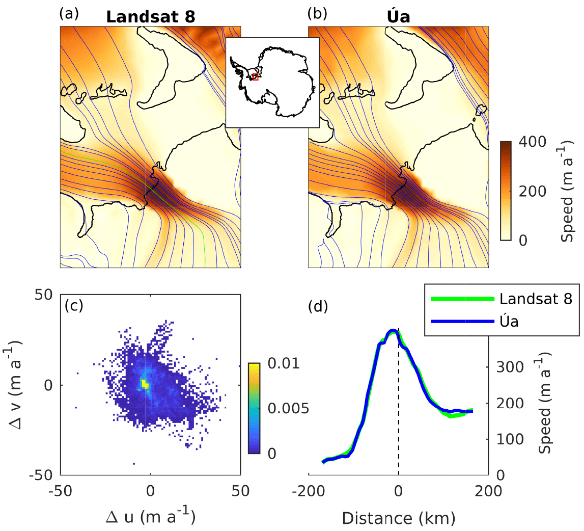
Figure 1Observed (Gardner et al., 2018) and modelled (b) ice speed in the region of Institute Ice Stream. The inset displays the location of the plotted area in Antarctica. Grounding lines are shown as black lines and streamlines are displayed in blue. Panel (c) shows a normalised bivariate histogram of the velocity residuals which are the differences between modelled and observed velocities within this area, that is, and , and u and v are the horizontal components of the surface velocity vector, respectively. Panel (d) shows an ice-speed profile along the central line of Institute Ice Stream that is indicated in green in (a).
When calculating grounding-line fluxes we interpolate nodal quantities of the computational mesh onto the (calculated) grounding line. The grounding line does not, as such, enter the numerical calculations made by our numerical ice flow model. As described in Sect. 2, it is the flotation mask – evaluated at the integration points – that determines the impact of the basal drag term. However, in a post-processing step we determine the positions of the grounding lines from the flotation mask. Our approximation of the grounding line is a piecewise linear curve, with each linear segment representing the grounding line within a given computational element (see Figs. S1 and B1). We then interpolate nodal values onto the central point of each linear segment. The same procedure is employed when calculating both analytical and modelled fluxes.
In Schoof (2007a, b), an expression for the grounding-line flux (q) of marine ice sheets is derived. While the analysis is primarily focused on a flow-line configuration where ice-shelf buttressing plays no role, Schoof (2007a) also estimates how the flux might be affected by a reduction θ in axial stress at the grounding line due to ice-shelf buttressing. The resulting analytical flux expression is
where q is the ice flux across the grounding line, h is the ice thickness, ρi the ice density, ρw the density of ocean water and g the gravitational acceleration (please note that in the related Eq. 17 of Gudmundsson, 2013 for the flux q there is a typo in the exponent of the basal slipperiness C). For grounded ice, the tangential component of the basal traction (τb) is related to the basal velocity (vb) through the Weertman-type sliding law
where C is the basal slipperiness, and m is the stress exponent, while deviatoric stresses τij and strain rates in ice flow are linked via Glen's flow law
with the second invariant of the deviatoric stress tensor, exponent n (often set to 3) and rate factor A. Here τij denote the components of the deviatoric stress tensor and the components of the strain rate tensor.
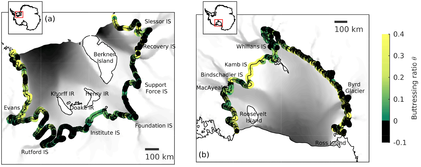
Figure 2Buttressing ratio θ1 along the grounding lines of Filchner–Ronne Ice Shelf (a) and Ross Ice Shelf (b). Insets indicate the ice shelves' locations in Antarctica. Regions where the grounding line is over-buttressed, that is, θ≤0, are displayed in black. Modelled speed is plotted in grey ranging up to 1500 m a−1. Grounding line and ice front locations are indicated in black. IS denotes ice streams; IR denotes ice rises or rumples.
As mentioned above, θ is a scalar quantity that describes the deviation in deviatoric axial stress at the grounding line from the unbuttressed situation. For an unbuttressed grounding line in one horizontal dimension (i.e. no variations in any quantities transverse to the flow direction) and assuming that the x axis of the coordinate system is aligned with the flow, we have τxx=τf where
which can be derived from the stress boundary condition at the calving front (see Appendix A). In the buttressed case, τxx is, however, no longer necessarily equal to τf, and θ is defined as
Here we have used the superscript 1HD to indicate that this definition of θ is only unambiguous in the one horizontal dimensional situation (1HD). In the more general two horizontal dimensional situation (2HD), where the flow direction is not necessarily aligned with the (horizontal) normal to the grounding line, several different definitions of θ are possible, and in the literature at least three different definitions of θ have been suggested. In the following we denote these by θ1, θ2, and θ3, with
where n1 is the normal to the grounding line, pointing horizontally outwards from the grounded ice into the ice shelf, and
and
where n2 is the direction of ice flow at the grounding line and
is the (horizontal) deviatoric stress tensor, and
is the tensor of resistive stresses. In the 1HD unbuttressed case where n1=n2, , and , all these three definitions of θ result in . The first definition (i.e. θ1) has, for example, been used by Gudmundsson (2013) to diagnose buttressing at the grounding line of an idealised set-up. The second definition has, for example, been used by Pollard and DeConto (2012), Thoma et al. (2014), and Pattyn (2017) as a flux condition, and the third one has been used by Fürst et al. (2016) to diagnose “flow buttressing” within Antarctic ice shelves. Note, however, that Pollard and DeConto (2012), Thoma et al. (2014, see Sect. 4.4), Fürst et al. (2016, see Supplementary Eq. 2), and Pattyn (2017; see Eq. 20) appear to use a different expression for τf, with , in which case in the unbuttressed case and θ in Eq. (6) must be replaced by 2θ.
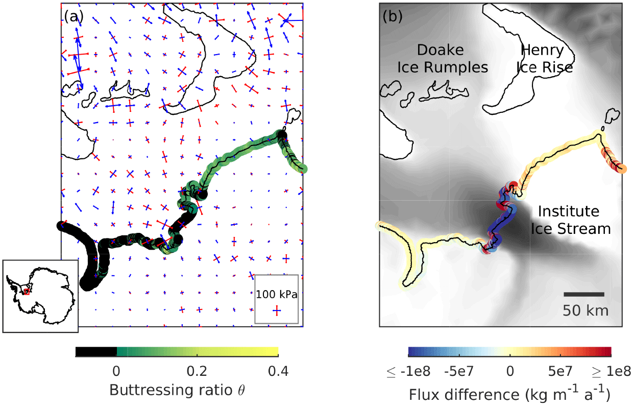
Figure 3Buttressing ratio and differences in grounding-line flux for Institute Ice Stream draining into the Filchner–Ronne Ice Shelf (location shown in inset). (a) Buttressing values θ1 are displayed along the grounding line and principle deviatoric stresses are shown with compression in red and extension in blue. The length of the vectors indicate the magnitude of each principle stress. (b) Differences between analytical and modelled fluxes and observed ice velocities ranging up to 500 m a−1 (Gardner et al., 2018). Analytical fluxes are set to 0 where θ1<0. Grounding-line positions are indicated in black.
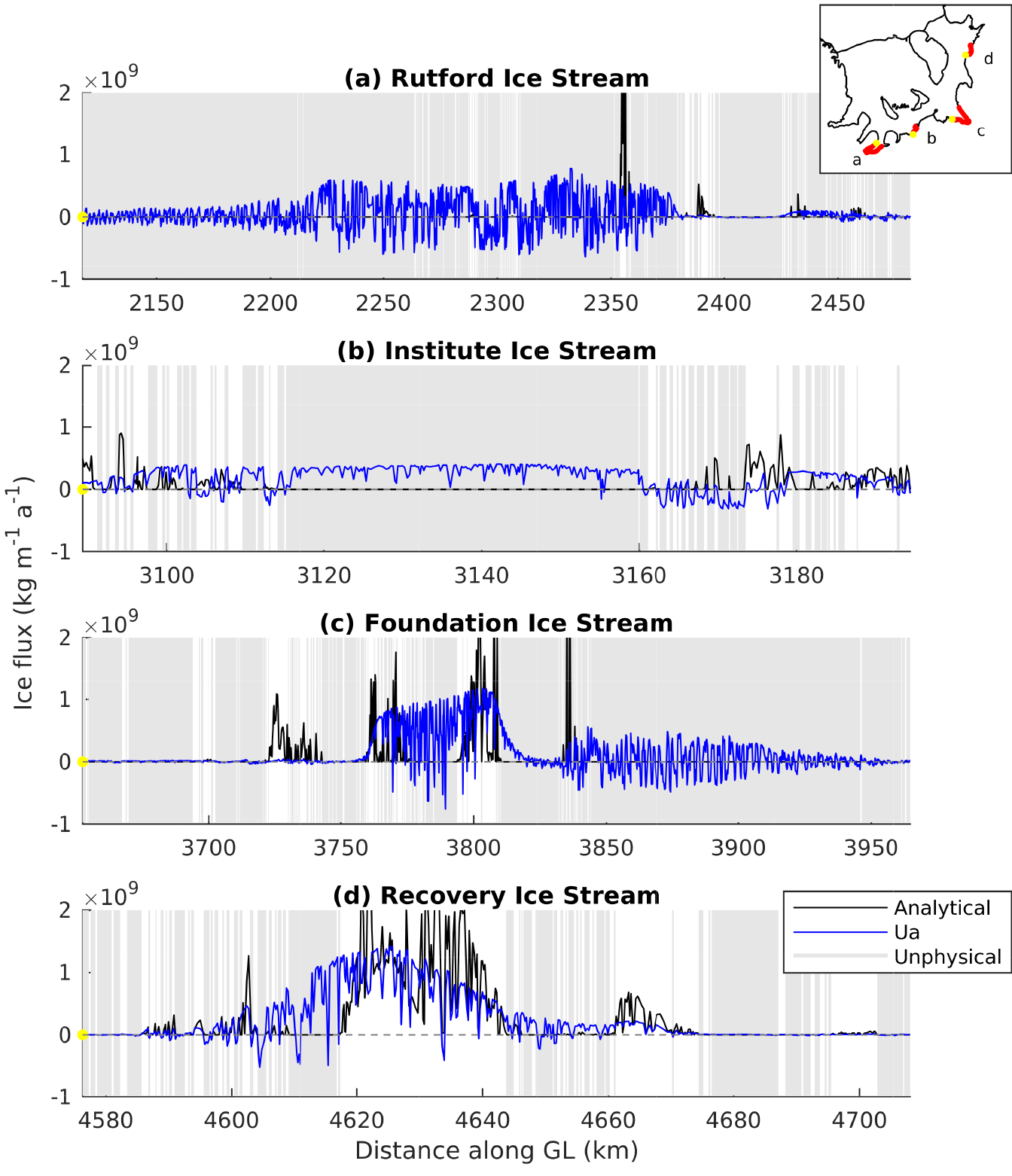
Figure 4Comparison of fluxes calculated with Úa (blue) and analytical fluxes (black) along the grounding lines of four major ice streams draining into the Filchner–Ronne Ice Shelf. Locations where the flux formula provides unphysical results are marked in grey. Plotted grounding-line segments are located as displayed in the inset with western margins indicated by a yellow dot.
The definition of θ1 is motivated by the form of the boundary condition at the calving front in the shallow ice-stream approximation (see Appendix A). For θ1=1 the normal traction at the grounding line equals that of a calving front. In the general 2HD situation, this same interpretation does not hold for the definitions of θ2 and θ3. If θ1>1 the ice shelf can be considered to be “pulling” the ice at the grounding line, while θ1<1 implies that the ice shelf causes a reduction in normal traction at the grounding line; i.e. the ice shelf “holds the ice back”. Note that, for all these three different definitions, it is possible for θ to become negative. If, however, a negative θ value is inserted into Eq. (6), the resulting value for the flux q is a negative or even a complex number for most combinations of n and m – a clear indication that the analytical flux formula fails in such situations. Only the specific combinations of n and m, such that for k∈ℕ (for instance the combination n=3 and m=2), “fix” the flux to a positive real number; however they introduce a non-substantiated dependency between the flow law and the sliding law. Furthermore, for these combinations and θ<0, enhanced buttressing inconsistently yields an increase in ice flux. Physically, θ1<0 corresponds to a situation where the traction vector at the grounding line points in upstream direction. One possible situation giving rise to θ1<0 would be τxx<0 while τyy=0, with x being the flow direction and the grounding line aligned with the y axis. In this case, the ice at the grounding line experiences compression in the along-flow direction and, hence, longitudinal strain rates are negative and ice velocities become smaller as the grounding line is approached from upstream direction. Another situation giving rise to θ1<0 is that of equal transversal compression and vertical extension of the ice column at the grounding line; i.e. while τxx=0.
From the numerically modelled stress field we calculate the buttressing parameter θ1 (given by Eq. 11) for all grounding lines of the Antarctic set-up described in Sect. 2.1. While here we focus on the buttressing parameter θ1, our findings are independent of the exact definition of θ, the choice of the sliding law exponent m, the mesh and the details of the inverse methodology applied (see Appendix B).
We find that the grounding lines of the Filchner–Ronne and Ross ice shelves are, in general, highly buttressed with buttressing values significantly different from unity (see Fig. 2). Typically, θ1≤0.4, and in many cases θ1<0. Among the ice streams of these two biggest ice shelves of the AIS, the dormant Kamb Ice Stream is the least buttressed one, with θ1≈0.4. Over all other ice streams θ values are even smaller. Negative θ values are also found over grounding-line segments located between active ice streams, for example along the grounding line running between the Rutford and Institute ice streams.
An example of an ice stream where θ1<0 over most of its grounding line is the Institute Ice Stream (see Figs. 3 and 4). Inspection of the velocity field in the vicinity of the grounding line of that ice stream reveals that ice flow velocities decrease with distance as the grounding line is approached from upstream direction (see also Fig. 1d). Consequently, both along-flow strain rates and along-flow deviatoric stresses are negative (compressive). This general feature of ice flow around the grounding line of Institute Ice Stream implies that its grounding line is “over-buttressed” with the traction vector at the grounding line pointing in an inland direction. Hence, independently of our numerical simulation of the stress field, it is clear that for this ice stream a negative value for θ is obtained.
As discussed in Sect. 3 the analytical flux formula (Eq. 6) is clearly not applicable in situations where θ becomes negative. As θ is found to become negative over large sections of the grounding lines of many the ice streams of the two largest Antarctic ice shelves, i.e. Ross and Filchner–Ronne ice shelves, it follows that the formula cannot be used to calculate grounding-line ice fluxes over significant parts of the AIS.
We furthermore compare analytical and numerically modelled grounding-line ice fluxes in all regions where θ1≥0, i.e. where the application of the analytical flux formula (Eq. 6) results in real-valued ice fluxes. In particular, we compare both the flux values pointwise along all grounding lines (Fig. 5) and the total cumulative fluxes over grounding lines of ice streams and ice shelves (Table 1). When comparing cumulative analytical fluxes, we are forced to assume values for those sections of grounding lines for which θ is negative (and q complex). There we assume q=0, which is equivalent to setting θ=0.
In general, we find significant differences between analytically calculated and numerically modelled flux values. Analytical fluxes are much lower than modelled in many locations of the Filchner–Ronne Ice Shelf, especially along the grounding lines of the Rutford, Institute and Moeller ice streams (Fig. 5). However, cumulative analytical fluxes over all grounding lines of the Filchner–Ronne Ice Shelf are about 30 % larger than modelled for θ1, and this difference is considerably larger for θ2 and θ3 (Table 1). A similar disagreement between analytical and modelled fluxes is found for the Siple Coast ice streams such as Bindschadler and MacAyeal ice streams, and for Byrd Glacier (Fig. 5b). For Ross Ice Shelf the overall difference is only 5 %, but, given the fact that θ1 is negative over significant sections of its grounding line (where we set the analytical flux values to zero), this agreement appears somewhat fortuitous.
For other ice shelves, cumulative fluxes are generally underestimated by the flux formula. Analytical fluxes for Pine Island Glacier and Thwaites Glacier, for example, deviate by −33 % and −52 % from the modelled fluxes, respectively. For George VI ice shelf, cumulative analytical fluxes are several times smaller than modelled ones (Table 1).
The analytical flux formula tends to strongly overestimate fluxes over grounding lines where ice flow is approximately tangential to the grounding line. The failure of the flux formula to correctly predict fluxes in such circumstances is not surprising, as the underlying assumptions of the formula are clearly not met in these situations. Nevertheless, this demonstrates the inherent conceptual difficulties in applying the formula to the Antarctic Ice Sheet.
Moreover, the analytical formula produces much higher spatial variability in fluxes than the numerically modelled ones. This can be clearly seen in Fig. 4, where analytical and modelled ice fluxes are plotted along the grounding lines of Rutford, Institute, Foundation and Recovery ice streams. Here, the grey background indicates sections of the respective grounding lines where the flux formula yields unphysical results. Variability in fluxes calculated with Úa occurs when ice flow is nearly aligned with the grounding line. We calculate fluxes within each triangular element using the normal of the piecewise-linear grounding-line curve, which may vary among individual line segments.
Table 1Ice flux integrated along the grounding lines of Antarctic ice shelves. QÚa denotes the modelled ice flux with Úa, Q1 was derived from the analytical flux formula based on θ1, Q2 based on θ2 and Q3 based on θ3, respectively. The last column shows the deviation of the analytical flux Q1 from the modelled QÚa.
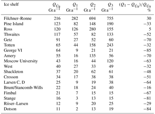

Figure 5Difference between the analytical and the modelled fluxes along the grounding lines of Filchner–Ronne Ice Shelf (a) and Ross Ice Shelf (b). Analytical fluxes are calculated based on θ1 defined in Eq. (11). In locations where the formula yields unphysical results, fluxes are set to zero. Grey arrows show the modelled ice flow. IS denotes ice streams; IR denotes ice rises or rumples. Grounding line and ice front locations are indicated in black.
We test the sensitivity of our analytical flux calculations to different degrees of regularisation (γs and γa), different values of the sliding law stress exponent (m) and relaxation of the ice geometry, for which our findings are summarised in Appendix B. Numerically modelled fluxes are, as expected, mostly independent of the value of the sliding law stress exponent m. This can be considered to be a consequence of the inversion procedure, which ensures that modelled velocity fields agree closely with measured data, independently of the value of m. On the other hand, analytically calculated flux values are highly sensitive to the value of m (see Fig. B3). For example, cumulative analytical fluxes for Filchner–Ronne Ice Shelf increase by about a factor of 5 as m is changed from 1 to 7, while numerically modelled fluxes change by less than 10 %. Numerically modelled fluxes are also insensitive to the exact degree of regularisation applied, whereas analytically calculated flux values change significantly (Fig. B5). The dependency of the analytically calculated fluxes on the amount of regularisation used in the numerical model is due to the impact regularisation has on modelled stresses and, therefore, on the value of θ.
We also compare analytical fluxes as calculated using the three different definitions (Eqs. 11, 12 and 13) for θ. While overall spatial variability of θ is similar for these three definitions, with all definitions giving rise to extended areas of negative θ values, the cumulative flux for the alternative definitions θ2 and θ3 are generally higher than for θ1 (see also Fig. B4). Extended negative θ values and large flux deviations are consistently found after a short relaxation period (see Figs. S6 and S7).
The analytical grounding-line flux formula Eq. (6) was derived for a flow-line configuration (Schoof, 2007a), and there is no reason to doubt its validity in that particular case. When applied to a flow-line configuration, many current ice-flow models employing the shallow ice-stream approximation (SSA) with Weertman-type sliding law, have demonstrated excellent agreement between modelled and analytical grounding-line fluxes (Pattyn et al., 2012). Ice fluxes and grounding-line positions calculated with the ice flow model Úa also agree closely with those predicted by Eq. (6), where such an agreement is to be expected. The inclusion of the buttressing parameter θ was used by Schoof (2007a) to illustrate the potential impacts of ice-shelf buttressing on ice flux, provided its effects were sufficiently small to not invalidate the basic assumption of a flow-line setting too strongly. However, we find that most of the grounding lines of the AIS are highly buttressed, with θ significantly different from unity. It seems likely that at least part of the reason that the analytical flux formula fails relates to the high degree of buttressing that we find to be characteristic for most Antarctic ice streams.
When applied to the current geometry and the current flow field of the AIS, the flux formula predicts either unphysical or highly inaccurate flux values when compared to modelled ones. While we have done the comparison with numerically modelled fluxes, a comparison with observed fluxes – calculated from measured surface velocities, observed grounding-line positions, and measured ice thicknesses – would not alter our conclusions as, due to our inversion procedure, observed and modelled surface velocities are in good agreement.
The strongest indication that the analytical flux formula fails when applied to the Antarctic Ice Sheet is arguably the fact that it predicts non-real valued fluxes over significant parts of Antarctic grounding lines. This happens whenever θ becomes negative. Although for specific combinations of n and m (such as n=3 and m=2) the resulting exponents in the flux formula are even numbers – in which case the analytical fluxes are always real positive numbers – the flux values are still unphysical (see Sect. 3). As we point out above, even a cursory inspection of the velocity field of the AIS suffices to show that θ is negative for a number of grounding lines (e.g. the Institute Ice Stream grounding line). Hence, the occurrence of negative θ values is not simply a feature of our particular numerical approach, but a general aspect of the current ice-flow regime of the AIS.
As analytical ice fluxes are strongly dependent on ice thickness (h) at the grounding line, they depend somewhat on the specifications of the numerical model: the exact location of the grounding line is influenced by the mesh resolution used by the model. The resulting error is an example of a discretization error that becomes smaller as the mesh is refined. Other numerical models using a different computational mesh may locate the grounding line differently and hence calculate different ice flux values. We tested the dependency of our modelled ice fluxes to grid resolution by using several different meshes – an example of two such meshes is given in Fig. B1 – and found none of our main conclusions to be affected by differences in mesh resolution.
As measured by the buttressing parameter θ1, almost all grounding lines of the AIS can be considered to be strongly buttressed with, in most cases, θ<0.4. Hence, theoretical concepts based on the assumption of none, or insignificant, ice-shelf buttressing may not apply to present-day Antarctica. One such theoretical prediction of considerable relevance for the possible future of the AIS relates to the stability of its grounding lines. In the absence of ice-shelf buttressing, grounding-line stability is predicted to be related to local bed slope (Schoof, 2007a, b, 2011; Thomas and Bentley, 1978; Weertman, 1974). However, in the presence of ice-shelf buttressing no such simple conclusions can be drawn (Goldberg et al., 2009; Gudmundsson, 2013; Gudmundsson et al., 2012; Pegler, 2016; Schoof et al., 2017). Possibly, rather than being dominated by local bed slope, the stability regime of the Antarctic Ice Sheet is to a leading order dependent on the properties of the ice shelves downstream of its grounding lines (e.g. geometry and structural integrity), as also supported by Pegler et al. (2013) and Haseloff and Sergienko (2018). Further work is needed to address the question of the stability of Antarctica's grounding lines.
In our study, we compare grounding-line ice fluxes obtained by an ice-sheet model with fluxes predicted by an analytical flux formula based on Schoof (2007a, b). The formula includes a parameter (θ) to account for ice-shelf buttressing, and the resulting flux is sometimes applied as a grounding-line flux condition in numerical simulations. We find that the formula results in unphysical and grossly inaccurate grounding-line fluxes for most of the AIS. We furthermore find that almost all Antarctic grounding lines are highly buttressed, suggesting that the underlying assumptions of the analytical flux formula are not met for the current configuration of the Antarctic Ice Sheet.
The data and code that support the findings of this study are available from the corresponding author upon request.
A derivation of the boundary condition at the calving front for the momentum equations in 2HD can be found in Cuffey and Paterson (2010) and van der Veen (1999), for example. At the calving face it holds that
where ncf=(nx, ny, 0) is the normal of the calving front pointing outwards, s is the ice surface, S is the sea-level and pw is hydrostatic pressure in the ocean . The balance in x direction reads
We can rewrite (since , and ). Under the assumptions of the cryostatic stress approximation, . The vertically integrated horizontal stress balance equals
since τxx, τyy, nx and ny do not vary vertically. Inserting this in Eq. (A1) yields the following:
A similar expression is obtained for the y direction. This can be abbreviated as
Following Gudmundsson (2013) we obtain the normal buttressing value, which compares the RHS and LHS of the equation above in the direction of the normal n at the grounding line:
In the case of a laterally uniform unconfined ice shelf with τyy=0 and τxy=0, this reduces to τxx∕τf.
A different approach that defines θ would be based on this vertically integrated stress boundary condition in 1HD with . In 1HD the normal at the grounding line is equal to the flow direction. In 2HD, this is not necessarily true. Thus, to generalize the longitudinal direction in the 1HD buttressing ratio, a choice needs to be made. The longitudinal direction can either be generalized as the normal at the grounding line (θ2) or as the flow direction (θ3).
We test the robustness of our findings with respect to the mesh, the sliding law stress exponent m, the definition of the buttressing parameter θ, the regularisation parameter γs and relaxation of the ice geometry. In a second pan-Antarctic set-up, based on a different mesh with quadratic base functions (instead of linear elements; see Fig. B1), we find a similar pattern of θ1≤0, which yields similar flux differences as exemplified in Fig. B2 for the Filchner–Ronne Ice Shelf. In this case, inversion was done for element-based basal slipperiness and ice softness (instead of inverting on a nodal basis) using a Bayesian methodology (instead of Tikhonov regularisation) and the MEASURES velocity data set (Rignot et al., 2011 instead of Landsat 8, Gardner et al., 2018). This set-up is further described in Reese et al. (2018). In this set-up, Bedmap2 bathymetry is not adjusted around the grounding line. This indicates that the exact location of the grounding line does not affect our findings.
For the Antarctic-wide set-up described in Sect. 2.1, we test the choice of the stress exponent m in the sliding law. Different choices of m=1, 3, 7 yield good agreement in modelled fluxes but large disagreement between analytical fluxes; see Fig. B3. Comparing shelf-wide integrated fluxes for major Antarctic ice shelves shows that the definitions θ2 and θ3 of the buttressing parameter also yield large deviations from the modelled fluxes; see Fig. B4. Similarly, we find that the choice of the regularisation parameter γs does not influence the results significantly; see Fig. B5. Extended areas of negative θ values and large flux deviations are consistently found after a short relaxation run; see Figs. S6 and S7. Our findings are hence independent of the details of numerical modelling choices.
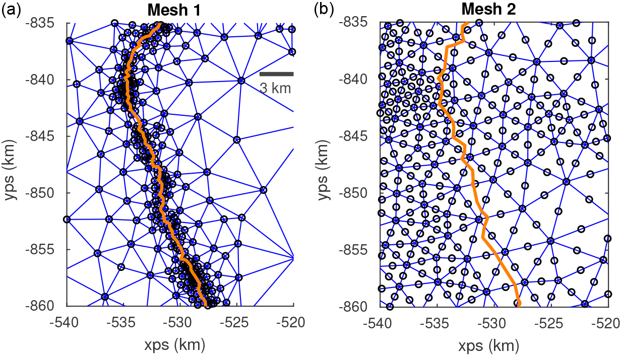
Figure B1Close-up of the Bindschadler grounding line for two different meshes. (a) Elements and nodes of the mesh presented in the main text. The mesh was refined, especially around the grounding line, and linear 3-node elements were employed. (b) An alternative mesh with 6-node elements with quadratic base functions. The grounding-line position is indicated in both meshes in orange.
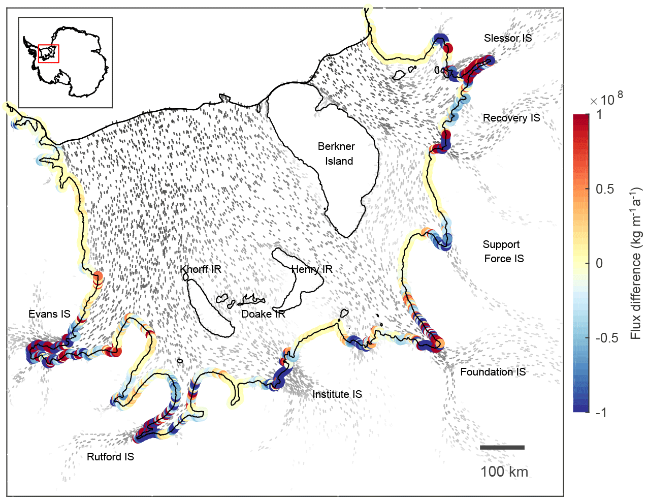
Figure B2Difference between formula-derived and modelled fluxes along the grounding lines of Filchner–Ronne Ice Shelf. In contrast to Fig. 5 a different mesh was employed (exemplified in the right panel in Fig. B1), the data assimilation was conducted using Bayesian inversion and based on the MEASURES velocity data set (Rignot et al., 2011). The analysis was done using quadratic elements. This Antarctic-wide set-up is described in more detail in Reese et al. (2018).
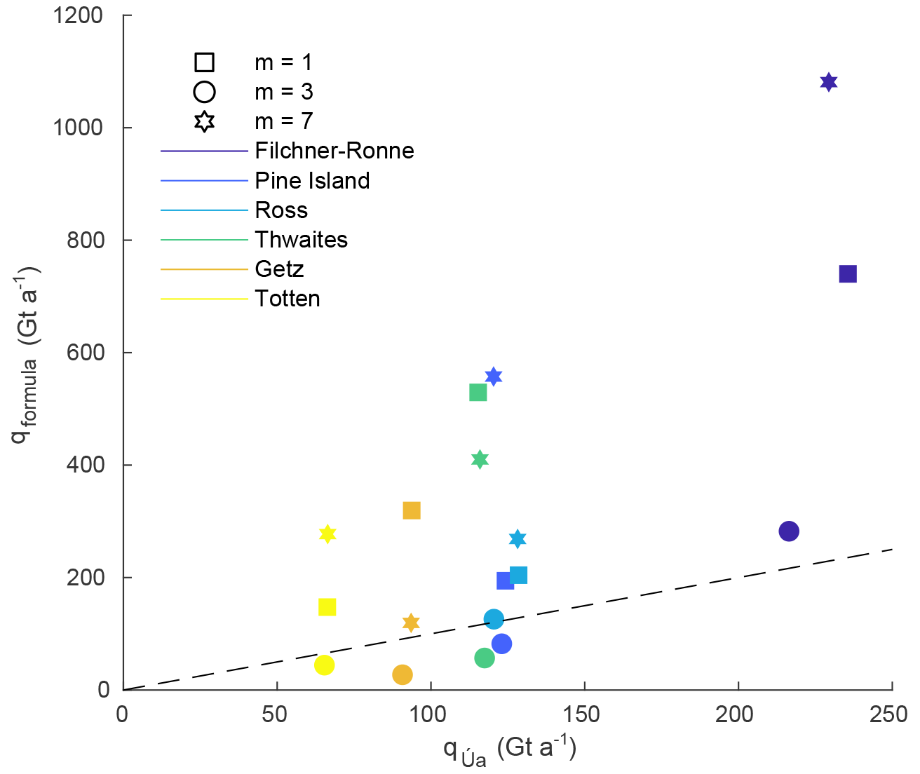
Figure B3Comparison of fluxes calculated with Úa (x axis) and with the analytical flux formula (y axis, using θ1), integrated along the grounding lines of the ice shelves indicated in the legend. Symbols indicate the different sliding law exponents m=1, 3, 7. All other parameters agree with the reference run (indicated by a circle). The dashed line shows where fluxes calculated with Úa and predicted by the formula would agree.
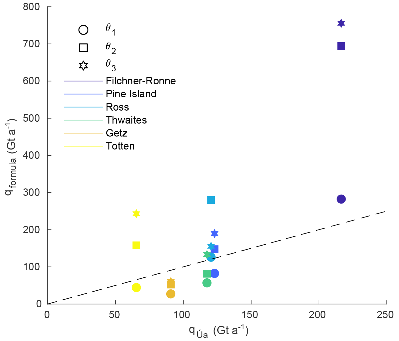
Figure B4Comparison of fluxes calculated with Úa (x axis) and with the analytical flux formula (y axis), integrated along the grounding lines of the ice shelves indicated in the legend. Symbols indicate the different definitions of θ as described in Sect. 3. All other parameters agree with the reference run (indicated by a circle). The dashed line shows where fluxes calculated with Úa and predicted by the formula would agree.
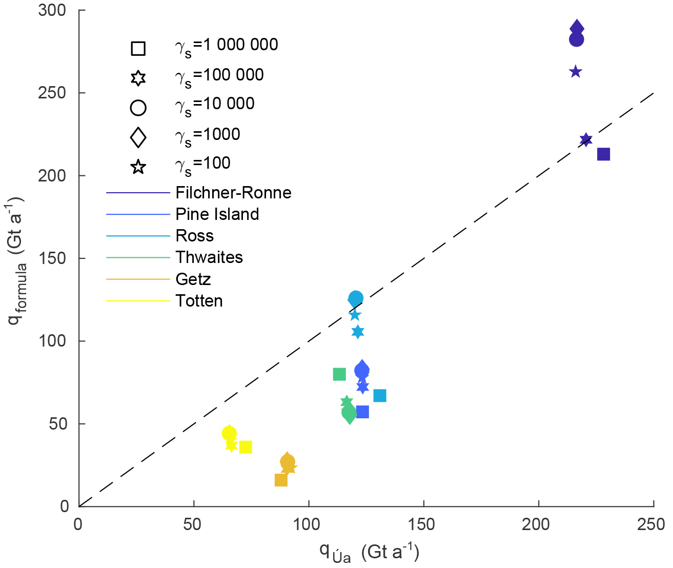
Figure B5Comparison of fluxes calculated with Úa (x axis) and with the analytical flux formula (y axis, using θ1), integrated along the grounding lines of the ice shelves indicated in the legend. Symbols indicate the different regularisation parameters γs. All other parameters agree with the reference run (indicated by a circle). The dashed line shows where fluxes calculated with Úa and predicted by the formula would agree.
The supplement related to this article is available online at: https://doi.org/10.5194/tc-12-3229-2018-supplement.
All authors designed the study. RR carried out the analysis based on an Antarctic set-up and using the ice-flow model Úa, both developed by GHG. RR prepared the manuscript with contributions from GHG and RW.
The authors declare that they have no conflict of interest.
We would like to thank Christian Schoof, the anonymous reviewer and the
editor Olivier Gagliardini for their helpful comments on the manuscript.
Ronja Reese was supported by the COMNAP Antarctic Research
Fellowship 2016–2017, the German Academic National Foundation, the
postgraduate scholarship programme of the state of Brandenburg and the
Evangelisches Studienwerk Villigst.
The article processing charges for this open-access
publication
were covered by the Potsdam Institute
for Climate Impact Research (PIK).
Edited by: Olivier Gagliardini
Reviewed by: Christian Schoof and one anonymous referee
Asay-Davis, X. S., Cornford, S. L., Durand, G., Galton-Fenzi, B. K., Gladstone, R. M., Gudmundsson, G. H., Hattermann, T., Holland, D. M., Holland, D., Holland, P. R., Martin, D. F., Mathiot, P., Pattyn, F., and Seroussi, H.: Experimental design for three interrelated marine ice sheet and ocean model intercomparison projects: MISMIP v. 3 (MISMIP+), ISOMIP v. 2 (ISOMIP+) and MISOMIP v. 1 (MISOMIP1), Geosci. Model Dev., 9, 2471–2497, https://doi.org/10.5194/gmd-9-2471-2016, 2016. a
Bindschadler, R., Choi, H., Wichlacz, A., Bingham, R., Bohlander, J., Brunt, K., Corr, H., Drews, R., Fricker, H., Hall, M., Hindmarsh, R., Kohler, J., Padman, L., Rack, W., Rotschky, G., Urbini, S., Vornberger, P., and Young, N.: Getting around Antarctica: new high-resolution mappings of the grounded and freely-floating boundaries of the Antarctic ice sheet created for the International Polar Year, The Cryosphere, 5, 569–588, https://doi.org/10.5194/tc-5-569-2011, 2011. a
Cornford, S., Martin, D., Lee, V., Payne, A., and Ng, E.: Adaptive mesh refinement versus subgrid friction interpolation in simulations of Antarctic ice dynamics, Ann. Glaciol., 57, 1–9, 2016. a
Cuffey, K. M. and Paterson, W. S. B.: The physics of glaciers, Academic Press, Elsevier Science, 2010. a
DeConto, R. M. and Pollard, D.: Contribution of Antarctica to past and future sea-level rise, Nature, 531, 591–597, 2016. a
De Rydt, J. and Gudmundsson, G. H.: Coupled ice shelf-ocean modeling and complex grounding line retreat from a seabed ridge, J. Geophys. Res.-Ea. Surf., 121, 865–880, https://doi.org/10.1002/2015JF003791, 2016. a
De Rydt, J., Gudmundsson, G., Rott, H., and Bamber, J.: Modeling the instantaneous response of glaciers after the collapse of the Larsen B Ice Shelf, Geophys. Res. Lett., 42, 5355–5363, 2015. a
Docquier, D., Perichon, L., and Pattyn, F.: Representing grounding line dynamics in numerical ice sheet models: recent advances and outlook, Surv. Geophys., 32, 417–435, 2011. a
Drouet, A. S., Docquier, D., Durand, G., Hindmarsh, R., Pattyn, F., Gagliardini, O., and Zwinger, T.: Grounding line transient response in marine ice sheet models, The Cryosphere, 7, 395–406, https://doi.org/10.5194/tc-7-395-2013, 2013. a
Feldmann, J., Albrecht, T., Khroulev, C., Pattyn, F., and Levermann, A.: Resolution-dependent performance of grounding line motion in a shallow model compared with a full-Stokes model according to the MISMIP3d intercomparison, J. Glaciol., 60, 353–360, 2014. a
Fretwell, P., Pritchard, H. D., Vaughan, D. G., Bamber, J. L., Barrand, N. E., Bell, R., Bianchi, C., Bingham, R. G., Blankenship, D. D., Casassa, G., Catania, G., Callens, D., Conway, H., Cook, A. J., Corr, H. F. J., Damaske, D., Damm, V., Ferraccioli, F., Forsberg, R., Fujita, S., Gim, Y., Gogineni, P., Griggs, J. A., Hindmarsh, R. C. A., Holmlund, P., Holt, J. W., Jacobel, R. W., Jenkins, A., Jokat, W., Jordan, T., King, E. C., Kohler, J., Krabill, W., Riger-Kusk, M., Langley, K. A., Leitchenkov, G., Leuschen, C., Luyendyk, B. P., Matsuoka, K., Mouginot, J., Nitsche, F. O., Nogi, Y., Nost, O. A., Popov, S. V., Rignot, E., Rippin, D. M., Rivera, A., Roberts, J., Ross, N., Siegert, M. J., Smith, A. M., Steinhage, D., Studinger, M., Sun, B., Tinto, B. K., Welch, B. C., Wilson, D., Young, D. A., Xiangbin, C., and Zirizzotti, A.: Bedmap2: improved ice bed, surface and thickness datasets for Antarctica, The Cryosphere, 7, 375–393, https://doi.org/10.5194/tc-7-375-2013, 2013. a
Fürst, J. J., Durand, G., Gillet-Chaulet, F., Tavard, L., Rankl, M., Braun, M., and Gagliardini, O.: The safety band of Antarctic ice shelves, Nat. Clim. Change, 6, 479–482, 2016. a, b, c, d
Gagliardini, O., Brondex, J., Gillet-Chaulet, F., Tavard, L., Peyaud, V., and Durand, G.: Brief communication: Impact of mesh resolution for MISMIP and MISMIP3d experiments using Elmer/Ice, The Cryosphere, 10, 307–312, https://doi.org/10.5194/tc-10-307-2016, 2016. a
Gardner, A. S., Moholdt, G., Scambos, T., Fahnstock, M., Ligtenberg, S., van den Broeke, M., and Nilsson, J.: Increased West Antarctic and unchanged East Antarctic ice discharge over the last 7 years, The Cryosphere, 12, 521–547, https://doi.org/10.5194/tc-12-521-2018, 2018. a, b, c, d
Geuzaine, C. and Remacle, J.-F.: Gmsh: A 3-D Finite Element Mesh Generator with Built-in Pre- and Post-Processing Facilities, 79, 1309–1331, 2009. a
Gladstone, R. M., Payne, A. J., and Cornford, S. L.: Parameterising the grounding line in flow-line ice sheet models, The Cryosphere, 4, 605–619, https://doi.org/10.5194/tc-4-605-2010, 2010. a
Gladstone, R. M., Payne, A. J., and Cornford, S. L.: Resolution requirements for grounding-line modelling: sensitivity to basal drag and ice-shelf buttressing, Ann. Glaciol., 53, 97–105, 2012. a
Goldberg, D., Holland, D., and Schoof, C.: Grounding line movement and ice shelf buttressing in marine ice sheets, J. Geophys. Res.-Ea. Surf., 114, F04026, https://doi.org/10.1029/2008JF001227, 2009. a, b
Gudmundsson, G. H.: Ice-shelf buttressing and the stability of marine ice sheets, The Cryosphere, 7, 647–655, https://doi.org/10.5194/tc-7-647-2013, 2013. a, b, c, d, e, f, g
Gudmundsson, G. H., Krug, J., Durand, G., Favier, L., and Gagliardini, O.: The stability of grounding lines on retrograde slopes, The Cryosphere, 6, 1497–1505, https://doi.org/10.5194/tc-6-1497-2012, 2012. a
Gudmundsson, G. H., De Rydt, J., and Nagler, T.: Five decades of strong temporal variability in the flow of Brunt Ice Shelf, Antarctica, J. Glaciol., 63, 164–175, https://doi.org/10.1017/jog.2016.132, 2017. a
Haseloff, M. and Sergienko, O. V.: The effect of buttressing on grounding line dynamics, J. Glaciol., 64, 417–431, https://doi.org/10.1017/jog.2018.30, 2018. a
Lenaerts, J. T. M., van den Broeke, M. R., van de Berg, W. J., van Meijgaard, E., and Kuipers Munneke, P.: A new, high-resolution surface mass balance map of Antarctica (1979–2010) based on regional atmospheric climate modeling, Geophys. Res. Lett., 39, l04501, https://doi.org/10.1029/2011GL050713, 2012. a
MacAyeal, D. R.: Large-scale ice flow over a viscous basal sediment: Theory and application to ice stream B, Antarctica, J. Geophys. Res.-Solid, 94, 4071–4087, 1989. a, b
MacAyeal, D. R. and Barcilon, V.: Ice-shelf response to ice-stream discharge fluctuations: I. Unconfined ice tongues, J. Glaciol., 34, 121–127, 1988. a
Morland, L. W.: Unconfined Ice-Shelf Flow, Springer Netherlands, Dordrecht, 99–116, https://doi.org/10.1007/978-94-009-3745-1_6, 1987. a, b
Pattyn, F.: Sea-level response to melting of Antarctic ice shelves on multi-centennial timescales with the fast Elementary Thermomechanical Ice Sheet model (f.ETISh v1.0), The Cryosphere, 11, 1851–1878, https://doi.org/10.5194/tc-11-1851-2017, 2017. a, b, c, d
Pattyn, F., Schoof, C., Perichon, L., Hindmarsh, R. C. A., Bueler, E., de Fleurian, B., Durand, G., Gagliardini, O., Gladstone, R., Goldberg, D., Gudmundsson, G. H., Huybrechts, P., Lee, V., Nick, F. M., Payne, A. J., Pollard, D., Rybak, O., Saito, F., and Vieli, A.: Results of the Marine Ice Sheet Model Intercomparison Project, MISMIP, The Cryosphere, 6, 573–588, https://doi.org/10.5194/tc-6-573-2012, 2012. a, b, c, d, e
Pattyn, F., Perichon, L., Durand, G., Favier, L., Gagliardini, O., Hindmarsh, R. C., Zwinger, T., Albrecht, T., Cornford, S., Docquier, D., Fürst, J. J., Goldberg, D., Gudmundsson, G. H., Humbert, A., Hütten, M., Huybrechts, P., Jouvet, G., Kleiner, T., Larour, E., Martin, D., Morlighem, M., Payne, A. J., Pollard, D., Rückamp, M., Rybak, O., Seroussi, H., Thoma, M., and Wilkens, N.: Grounding-line migration in plan-view marine ice-sheet models: results of the ice2sea MISMIP3d intercomparison, J. Glaciol., 59, 410–422, https://doi.org/10.3189/2013JoG12J129, 2013. a, b
Pattyn, F., Favier, L., Sun, S., and Durand, G.: Progress in numerical modeling of Antarctic ice-sheet dynamics, Curr. Clim. Change Rep., 3, 174–184, 2017. a
Pegler, S. S.: The dynamics of confined extensional flows, J. Fluid Mech., 804, 24–57, 2016. a
Pegler, S. S., Kowal, K. N., Hasenclever, L. Q., and Worster, M. G.: Lateral controls on grounding-line dynamics, J. Fluid Mech., 722, https://doi.org/10.1017/jfm.2013.140, 2013. a
Pollard, D. and DeConto, R. M.: Description of a hybrid ice sheet-shelf model, and application to Antarctica, Geosci. Model Dev., 5, 1273–1295, https://doi.org/10.5194/gmd-5-1273-2012, 2012. a, b
Reese, R., Gudmundsson, G. H., Levermann, A., and Winkelmann, R.: The far reach of ice-shelf thinning in Antarctica, Nat. Clim. Change, 8, 53–57, 2018. a, b, c, d
Rignot, E., Mouginot, J., and Scheuchl, B.: Ice flow of the Antarctic ice sheet, Science, 333, 1427–1430, 2011. a, b
Ritz, C., Edwards, T. L., Durand, G., Payne, A. J., Peyaud, V., and Hindmarsh, R. C.: Potential sea-level rise from Antarctic ice-sheet instability constrained by observations, Nature, 528, 115–118, 2015. a
Royston, S. and Gudmundsson, G. H.: Changes in ice-shelf buttressing following the collapse of Larsen A Ice Shelf, Antarctica, and the resulting impact on tributaries, J. Glaciol., 62, 905–911, https://doi.org/10.1017/jog.2016.77, 2016. a
Schoof, C.: Ice sheet grounding line dynamics: Steady states, stability, and hysteresis, J. Geophys. Res.-Ea. Surf., 112, F03S28, https://doi.org/10.1029/2006JF000664, 2007a. a, b, c, d, e, f, g, h, i, j
Schoof, C.: Marine ice-sheet dynamics. Part 1. The case of rapid sliding, J. Fluid Mech., 573, 27–55, 2007b. a, b, c, d
Schoof, C.: Marine ice sheet dynamics. Part 2. A Stokes flow contact problem, J. Fluid Mech., 679, 122–155, 2011. a
Schoof, C., Davis, A. D., and Popa, T. V.: Boundary layer models for calving marine outlet glaciers, The Cryosphere, 11, 2283–2303, https://doi.org/10.5194/tc-11-2283-2017, 2017. a
Seroussi, H., Morlighem, M., Rignot, E., Mouginot, J., Larour, E., Schodlok, M., and Khazendar, A.: Sensitivity of the dynamics of Pine Island Glacier, West Antarctica, to climate forcing for the next 50 years, The Cryosphere, 8, 1699–1710, https://doi.org/10.5194/tc-8-1699-2014, 2014. a
Thoma, M., Grosfeld, K., Barbi, D., Determann, J., Goeller, S., Mayer, C., and Pattyn, F.: RIMBAY – a multi-approximation 3D ice-dynamics model for comprehensive applications: model description and examples, Geosci. Model Dev., 7, 1–21, https://doi.org/10.5194/gmd-7-1-2014, 2014. a, b, c, d
Thomas, R. H. and Bentley, C. R.: A Model for Holocene Retreat of the West Antarctic Ice Sheet, Quatern. Res., 10, 150–170, https://doi.org/10.1016/0033-5894(78)90098-4, 1978. a
van der Veen, C.: Fundamentals of Glacier Dynamics, Geomorphology, 36, 261–262, 1999. a
Weertman, J.: Stability of the junction of an ice sheet and an ice shelf, J. Glaciol., 13, 3–11, 1974. a
- Abstract
- Introduction
- Model description
- Ice-shelf buttressing and grounding-line ice flux
- Results
- Discussion
- Conclusions
- Code and data availability
- Appendix A: Vertically integrated stress boundary condition at a free calving front
- Appendix B: Consistent results using different model parameters
- Author contributions
- Competing interests
- Acknowledgements
- References
- Supplement