2.1 AltiKa

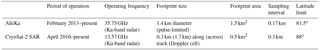
The SARAL/AltiKa satellite (herein referred to as AltiKa), was launched in spring 2013 as a joint mission between the Centre National d'Etudes Spatiales (CNES) and the Indian Space Research Organisation (ISRO). AltiKa's pulse-limited Ka-band radar altimeter, which operates at a central frequency of 35.75 GHz, retrieves surface elevations up to 81.5^∘ latitude. Armitage and Ridout (2015) used a “Gaussian plus exponential” retracker to retrieve lead elevations (after Giles et al., 2007) and a 50 % threshold retracker over floes. AltiKa freeboard data used in this study are derived using the same processing algorithm, and the reader is referred to the Supplement in Armitage and Ridout (2015) for further details.

Table 1AltiKa and CS-2 (SAR mode) operation characteristics.

Download Print Version | Download XLSX

2.2 CryoSat-2

CS-2 was launched by the European Space Agency in 2010, tasked with the specific role of monitoring the Earth's cryosphere. The satellite has an orbital inclination of 88^∘, giving it far better coverage over the poles than previous radar altimeters, and unlike AltiKa, CS-2 employs along-track SAR processing to achieve an along-track resolution of approximately 300 m, improving the sampling of smaller floes and making it less susceptible to snagging from off-nadir leads (Wingham et al., 2006). As with AltiKa, lead elevations are retrieved using the Gaussian plus exponential model fit and for floes a 70 % threshold retracker was determined as offering the best average elevation from the CS-2 unique SAR waveforms (Wingham et al., 2006). The CS-2 freeboard data used in this study were processed by the Centre for Polar Observation and Modelling (CPOM) and readers are referred to Tilling et al. (2018) for further details on the method.

2.3 Sources of AltiKa vs. CryoSat-2 freeboard bias

We define AltiKa vs. CS-2 freeboard bias as the portion of the AltiKa minus CS-2 freeboard difference that does not originate from the difference in snow penetration of the two radars. In line with radar theory (Rapley et al., 1983) and in light of recent findings by Guerreiro et al. (2017), we expect such a bias to be the result of the difference in footprint sizes between the two altimeters and the consequences of this during freeboard processing. The differences between AltiKa and CS-2 of interest to this study are summarised in Table 1.

In an initial stage of AltiKa and CS-2 freeboard processing, waveforms are classified as either lead or floe according to thresholds for pulse peakiness, defined as

where N is the number of range bins above the “noise floor” (calculated as the mean power in range bins 10–20), p_max is the maximum waveform power (the “highest peak”), and Σ_i p_i is the sum of the power in all range bins above the noise floor (Peacock and Laxon, 2004). It should also be noted that further waveform parameters are used to identify lead and floes: stack standard deviation (SSD) for CS-2 (Tilling et al., 2018) and backscatter coefficient σ₀ for AltiKa (Armitage and Ridout, 2015). Since PP is the criterion shared by both, it is the focus of our discussion here.

Waveforms originating from smooth, specular leads demonstrate a rapid rise in power followed by a sharp drop off, giving them a high PP. Returns from floes typically demonstrate a more gradual rise in power and slower drop-off, equivalent to a lower PP. PP can therefore be used to distinguish floe and lead returns and eliminate those not clearly identifiable as one or the other. For AltiKa (CS-2), waveforms with PP less than 5 (9) are designated as originating from ice floes. Waveforms with PP greater than 18 are classified as leads for both satellites (Armitage and Ridout, 2015; Tilling et al., 2018).

Waveforms that exhibit a mixture of scattering behaviour will have a PP in the “ambiguous” range (5 < PP < 18 for AltiKa and 9 < PP < 18 for CS-2) and are discarded. Since AltiKa has a larger footprint, its waveforms are more likely to be ambiguous and therefore discarded than CS-2, which can resolve smaller floes within the same region. The result of this is a bias in AltiKa towards higher freeboards (only larger floes, which tend to be thicker, are captured), especially over seasonal lead-dense areas.

The impact of surface roughness on pulse-limited altimetry is well documented (Chelton et al., 2001; Raney, 1995; Rapley et al., 1983). Generally, a rougher surface leads to dilation of the footprint and a widening of the leading edge of the waveform return. For a homogeneously rough surface with a Gaussian surface elevation distribution, the 50 % power threshold represents the mean surface elevation within the pulse-limited footprint. However, for a heterogeneously rough surface, such as that of multi-year sea ice, the waveform leading edge can take a complex shape where the half-power point does not necessarily represent the average elevation within the footprint and using a 50 % threshold retracker might lead to a biased surface height retrieval (Chelton et al., 2001; Raney, 1995; Rapley et al., 1983). Despite its along-track Doppler processing and effective sharpening of the waveform response, CS-2 may also be susceptible to an elevation bias due to surface roughness. This was demonstrated by Kurtz et al. (2014) who advocate the use of a physical model retracker in order to better resolve CS-2 surface elevation.

AltiKa is also more sensitive than CS-2 to off-nadir ranging to leads due to its larger footprint. This occurs when an off-nadir lead dominates the waveform response, resulting in an overestimate of the range to the lead, an underestimate of sea surface height, and a positive bias on the local floe freeboard (Armitage and Davidson, 2014). To minimise this effect, lead waveforms for AltiKa are discarded if their backscatter per unit area, σ⁰, is less than 24 dB, under the assumption that off-nadir leads return less power to the antenna compared with those at nadir (Armitage and Ridout, 2015). However, it is unlikely that this criterion eradicates the problem altogether and we expect that the freeboard bias due to snagging is larger in the AltiKa data compared to CS-2.

To overcome the CS-2 vs. AltiKa freeboard bias, Guerreiro et al. (2016) employed degraded SAR mode CS-2 data in their comparison, where the synthetic Doppler beams are not aligned in time and are summed incoherently to obtain a pseudo-pulse-limited echo. Since this offers a footprint and waveform more closely resembling that of AltiKa, it was assumed that observed elevation differences between AltiKa and degraded CS-2 were the result of differences in snow penetration only.

Rather than separating the contributions of freeboard difference in this way, we here introduce an approach that calibrates AltiKa freeboard to align it to the snow surface and CS-2 to the ice–snow interface (we assume in general that CS-2 penetrates further than AltiKa due to its longer wavelength, Ulaby et al., 1984). As such, penetration properties and sources of freeboard bias are corrected in one step without needing to consider the contribution of each.

While the comparisons of Guerreiro et al. (2016) derived snow depths with those from OIB are encouraging, the assumption of zero penetration for AltiKa and full penetration for CS-2 introduces limitations and is counter to observational results (Armitage and Ridout, 2015; Giles and Hvidegaard, 2006; Nandan et al., 2017; Willatt et al., 2011) – and indeed their own model simulations – in support of a spatially and temporally variable penetration depth as a function of snow characteristics. Here we offer a methodology that both accounts for variable AltiKa and CS-2 snow penetration and is simple; freeboard data can be utilised as they are, without reprocessing. This is in contrast to the method of Guerreiro et al. (2016) which relies on the ability to process one of the satellite data sets to achieve comparable footprints and thus alleviate the biases due to the difference in sampling areas. It is fortunate that CS-2 pseudo-LRM (Low Resolution Mode) has a similar footprint to AltiKa (1.7 km diameter and 1.4 km diameter respectively), but how, for example, could the methodology be applied to CS-2 and ICESat-2 in order to retrieve contemporary snow depth estimates once AltiKa ceases functionality? Although herein we demonstrate our methodology applied to the AltiKa and CS-2 satellites, our intention is to outline an approach that can be applied more broadly. Given the recent launch of ICESat-2 and the unique opportunity that its coincidence with CS-2 provides, we demonstrate the applicability of our method to the Envisat (same operating frequency as CS-2) and ICESat satellites.

2.4 Operation IceBridge

In order to evaluate the deviation of each satellite's retrieved elevation from its “expected” dominant scattering horizon (the snow surface for AltiKa and the snow–ice interface for CS-2), we use laser freeboard and snow depth from NASA's 2013–2016 OIB spring campaigns. It is important to note that a variety of research groups process OIB snow radar data in different ways, and the results vary significantly (for the 2013–2015 period, campaign-average snow depths differ by up to 7 cm over first-year ice and 12 cm over multi-year ice; Kwok et al., 2017). Evidently the lack of a singular, robust independent data set presents a limitation to our methodology since our aim is to calibrate to the “true” snow and ice freeboards. In an attempt to offer the best Dual-altimeter Snow Thickness product possible, we employ OIB snow depths processed from snow radar data by the NASA Jet Propulsion Laboratory (JPL), as these demonstrated best agreement with ERA-interim reanalysis data and the Warren climatology for the 2013–2015 period (Kwok et al., 2017). We return to a discussion on this limitation in Sect. 3.2.

Our methodology requires a comparison of CS-2 radar freeboard with OIB radar freeboard. To calculate this we use snow freeboard, retrieved using the OIB ATM (Airborne Topographic Mapper) laser altimeter, from which snow depth can be subtracted. Currently, ATM freeboard data are only available from the National Snow and Ice Data Center (NSIDC), and for the 2014–2016 period these exist solely in Quick Look format: a first release, expedited version, which demonstrates reduced accuracy compared with the final release products (Kurtz, 2014). In the interest of consistency we also use the ATM laser freeboard Quick Look product for 2013.

Sea ice freeboard f_i is calculated by subtracting OIB JPL snow depth h_s from OIB Quick Look laser freeboard f_l. Ice freeboard is then converted to radar freeboard f_r by

The OIB radar freeboard represents the freeboard that would be retrieved by a satellite altimeter whose pulse penetrated through to the ice–snow interface (Armitage and Ridout, 2015). We choose a value of c∕c_s of 1.28 after Kwok (2014). In the following discussion, AltiKa and CS-2 freeboard refers to the radar freeboard, that is the freeboard retrieved by the satellite before the correction for light propagation through the snowpack is applied.

2.5 AltiKa calibration with Operation IceBridge

For each day of the three spring campaigns 2013–2015, OIB laser freeboard data are averaged onto a 2^∘ longitude × 0.5^∘ latitude grid. Grid cells containing less than 50 individual points are discarded to remove speckle noise. Along-track AltiKa freeboard and PP data for the ±10 days surrounding the campaign day are then averaged onto the same grid, and grid cells with less than 50 points are similarly discarded. This grid and time window were chosen because they produced the maximum number of grid cells where a grid cell must contain at least 50 airborne and satellite points.

Satellite freeboard and PP grids are then interpolated at the average position of the OIB data within each valid OIB grid cell. Further, high resolution (10 km gridded) ice type data from the EUMETSAT Ocean and Sea Ice Satellite Application Facility (OSI SAF, http://www.osi-saf.org, last access: 1 March 2018) are interpolated at the same point to determine whether multi-year or seasonal ice is being sampled. The value Δf_AK, defined as the ATM laser freeboard minus the AltiKa freeboard and plotted against AltiKa PP, is shown in Fig. 1. Data from 2013, 2014, and 2015 and their corresponding linear regression fits are plotted in red, blue, and grey respectively to demonstrate year to year consistency. Multi-year and first-year ice are distinguished by star and square markers in order to illustrate the variation of PP, and thus roughness, with ice type.

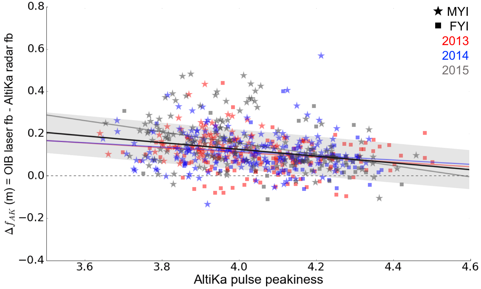
Figure 1The value Δf_AK, defined as the OIB laser freeboard minus the AltiKa radar freeboard, plotted against AltiKa pulse peakiness, for the OIB spring campaigns of 2013 (red), 2014 (blue), and 2015 (grey). Multi-year and first-year ice are plotted with stars and squares respectively, and the horizontal grey dashed line marks zero. The combined (all years) linear regression fit (CLRF), shown by the black line, has a slope of −0.16 and an intercept of 0.76. The shaded area around the CLRF shows the 68 % prediction interval, corresponding to a standard error (SE) on Δf_AK of 9.4 cm. Please note that fb is freeboard.

Download

The combined (all years) linear regression fit (CLRF) is shown by the black line and has slope of −0.16 and intercept of 0.76. The shaded area shows the 68 % prediction interval for the CLRF, corresponding to a standard error (SE) on Δf_AK of 9.4 cm. The CLRF is greater than zero for most PPs, implying that the freeboard needs to be increased to align with the snow–air interface, though more so (∼0.2 m) for low peakiness values (rougher ice) than for high peakiness values (smoother ice), where the correction approaches zero. This suggests that freeboard over rough ice is biased low, which could be attributed to difficulty in identifying the average footprint surface elevation as outlined in Sect. 2.3. It could also suggest that AltiKa exhibits greater snow penetration over rough ice than seasonal ice, in support of the assumption that (i) rough, multi-year ice has a thicker snow cover and (ii) seasonal ice is likely subject to brine wicking, which prevents radar propagation through the snow (Nandan et al., 2017). Ultimately we cannot separate the influence of individual sources of bias and physical penetration, and therefore, these observations are purely speculative.

2.6 CS-2 calibration with Operation IceBridge

The procedure for calibrating CS-2 with OIB is identical to that outlined above for AltiKa, but here Δf_CS is defined as the OIB radar freeboard (see Sect. 2.4) minus the CS-2 radar freeboard. For consistency and comparability with AltiKa, we remove CS-2 data above 81.5^∘ N from our analysis. The value Δf_CS is plotted against CS-2 PP and shown in Fig. 2. The CLRF, shown by the black line, has a slope of 0.06 and a negative intercept of −0.46. As before, the shaded area around the CLRF shows the 68 % prediction interval, and corresponds to a ±8.4 cm uncertainty (1 standard error) on Δf_CS.

For the entire CS-2 PP range, the CLRF is negative. It is most negative at lower PP, indicating that the CS-2 freeboard lies higher above the snow–ice interface over rough ice. This is in agreement with rougher ice exhibiting thicker snow cover and the radar pulse therefore being limited from getting as close to the snow–ice interface, where the snow is thinner. This deviation could also be the result of a failure of the empirical retracker to retrieve accurate surface elevation over rough ice, as demonstrated by Kurtz et al. (2014). As before, since we cannot separate the influence of individual sources of bias and physical penetration, these suggestions are speculative.

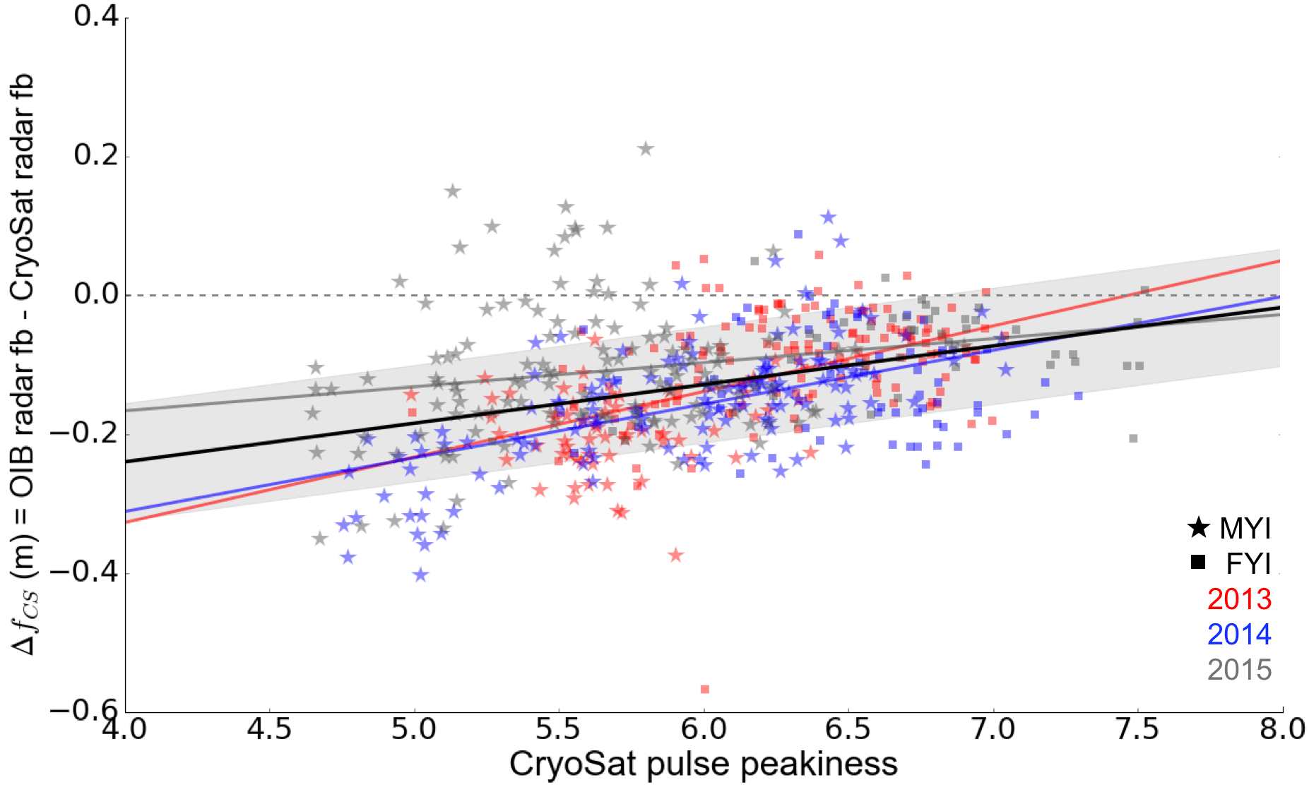
Figure 2The value Δf_CS, defined as the OIB theoretical radar freeboard minus the CS-2 radar freeboard, plotted against CS-2 pulse peakiness, for the OIB spring campaigns of 2013 (red), 2014 (blue), and 2015 (grey). Multi-year and first-year ice are plotted with stars and squares respectively, and the horizontal grey dashed line marks zero. The combined (all years) linear regression fit (CLRF), shown by the black line, has a slope of 0.06 and an intercept of −0.46. The shaded area around the CLRF shows the 68 % prediction interval, corresponding to a standard error (SE) on Δf_CS of 8.4 cm. Please note that fb is freeboard.

Download

3.1 Case study November 2015–April 2016

To derive snow depth, along-track freeboard measurements for AltiKa and CS-2 are calibrated as a function of PP according to the combined linear regression fits derived in the previous section and then averaged onto a 1.5^∘ longitude by 0.5^∘ latitude monthly grids. A finer grid resolution than for the calibration analysis is afforded given the coverage of 1 month's worth of data as compared to the 21 days (±10 days window) averaged previously. The calibrated CS-2 freeboard is subtracted from the calibrated AltiKa freeboard and multiplied by a factor of c_s∕c = 0.781 to convert to snow depth. Figure 3 summarises the retrieved monthly dual-altimeter snow thicknesses from November 2015 to April 2016. The delineation of multi-year and first-year ice is shown by the dashed black lines, adapted from OSI SAF Quicklook daily sea ice type maps for the 15th day of each month, available at http://osisaf.met.no/p/osisaf_hlprod_qlook.php?prod=Ice-Type&area=NH (last access: 1 March 2018).

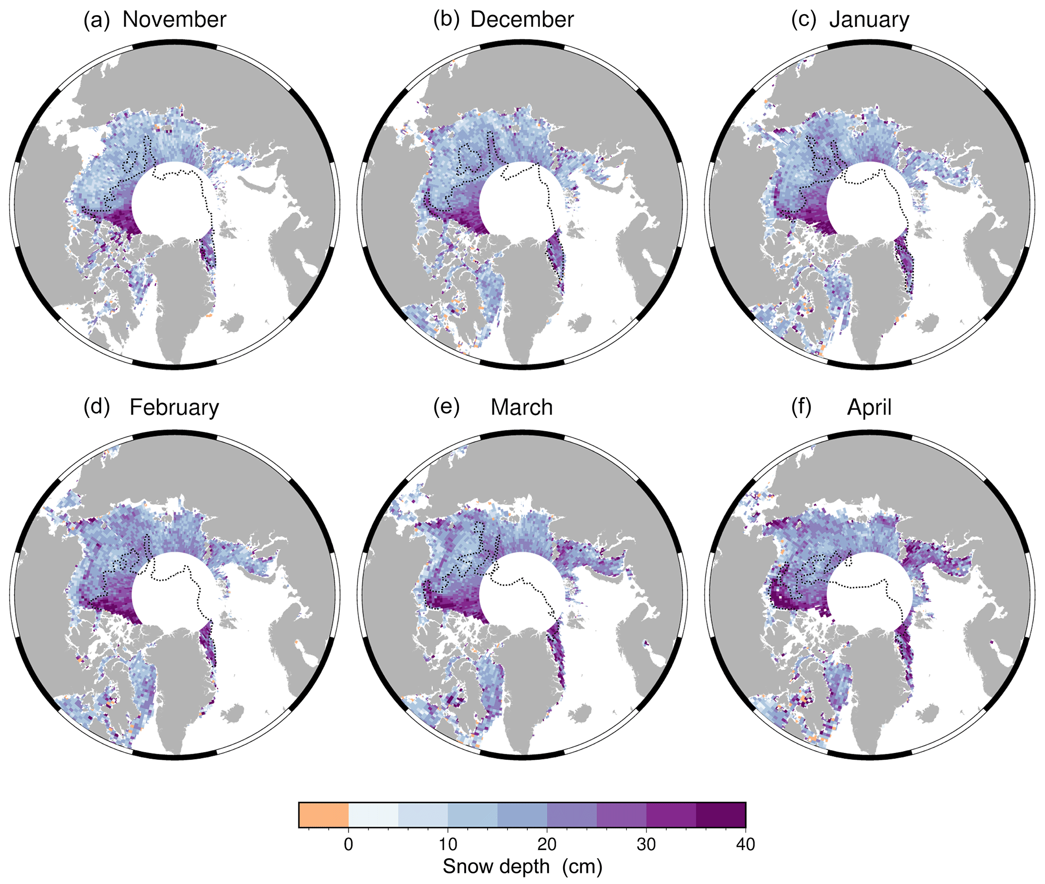
Figure 3Monthly snow depths for the growth season November 2015 (a) to April 2016 (f), derived from the AltiKa minus CS-2 calibrated freeboard. The multi-year ice boundary for each month is shown by the dashed black line, adapted from the OSI SAF Quicklook sea ice type map for the 15th day of the month, available at http://osisaf.met.no/p/osisaf_hlprod_qlook.php?prod=Ice-Type&area=NH (last access: 1 March 2018).

Download

Spatial distribution of snow depth follows the expected pattern of thin snow cover over seasonal ice (up to 25 cm) and thicker snow over multi-year ice (30–40 cm) (Warren et al., 1999), which in recent years is limited to regions north of the Canadian Archipelago (CAA) and Greenland and the Fram Strait. However, seasonal deposition of snow occurs between November and April, corresponding with the locations of predominant cyclone tracks in winter (e.g. the Aleutian Low on the Pacific side and the North Atlantic storm tracks). In particular, snow predominantly accumulates within the Chukchi Sea, and within the Kara, Barents, and eastern Greenland seas. As well as precipitation events, ice drift governs snow distribution through the advection of snow-loaded sea ice parcels around the ocean. Therefore, in order to understand the seasonal evolution of the snow cover, we compare snow depth maps with monthly sea ice motion vectors from the National Snow and Ice Data Center (NSIDC, available at https://daacdata.apps.nsidc.org, last access: 23 February 2018), shown in Fig. 4. We expect snow accumulation west of Banks Island in the CAA is the result of westward transport of multi-year ice by the Beaufort Gyre. Snow depths in the Kara Sea appear high given the advection of ice out of this region throughout the season; however, we cannot rule out anomalous precipitation events. Typically 20–40 extreme cyclones occur each winter within the North Atlantic, but in recent years there has been a trend towards increased frequency of cyclones, particularly near Svalbard (Rinke et al., 2017). These cyclones, while they transport heat and moisture into the Arctic and may impact the sea ice edge location (Boisvert et al., 2016; Ricker et al., 2017), can also be associated with increased precipitation.

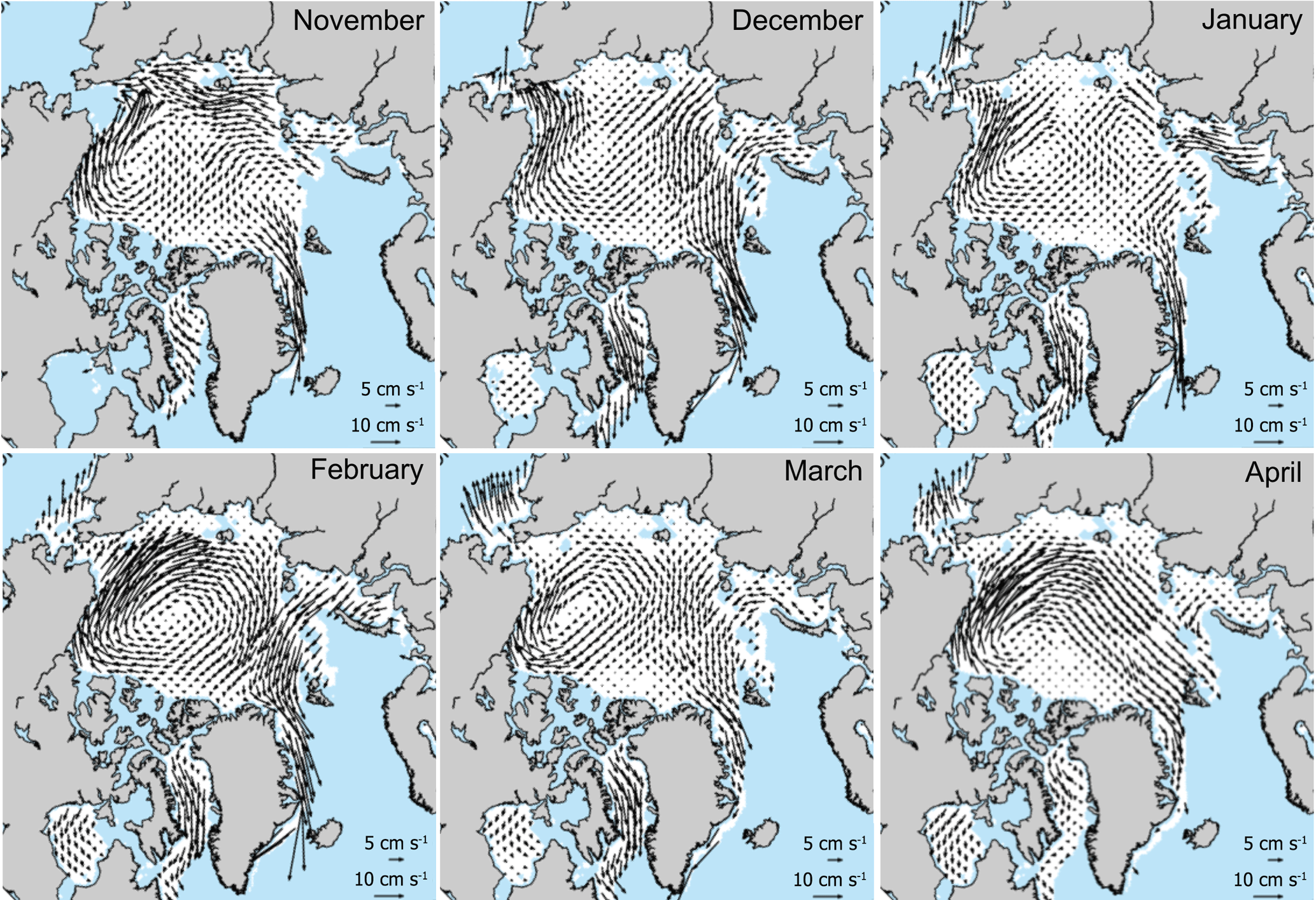
Figure 4NSIDC November 2015 to April 2016 monthly mean sea ice drift vectors. Adapted from images retrieved from https://daacdata.apps.nsidc.org/pub/DATASETS/nsidc0116_icemotion_vectors_v3/browse/north/ (last access: 23 February 2018).

Download

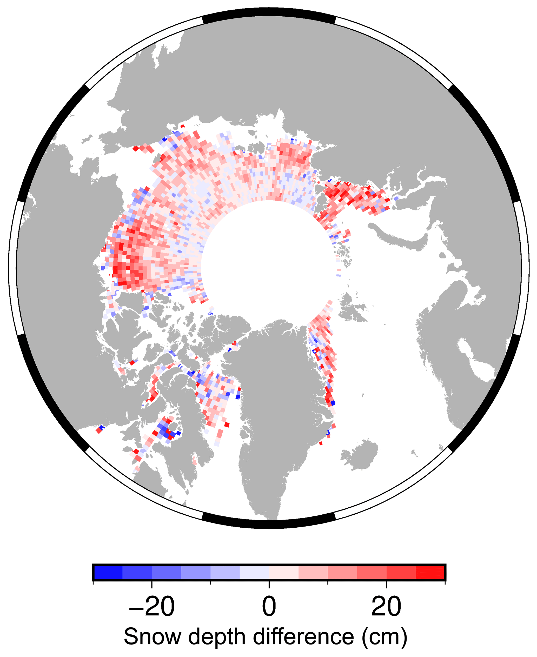
To understand where greatest accumulation of snow occurs over the season, we also plot the difference between November 2015 and April 2016 snow depth in Fig. 5. Snow accumulation is highest in the western Beaufort Sea, in particular adjacent to the coast of Canada. We attribute this to the advection of snow-loaded multi-year ice by the Beaufort Gyre, supported by the visible shift of the multi-year ice boundary through the season (Fig. 3). Accumulation also occurs in the Fram Strait, which we expect to be the result of southward advection of multi-year ice from the central Arctic Ocean in December and April, as well as snow deposition from the North Atlantic Storm tracks. High accumulation in the southern Chukchi Sea could also be explained by strong advective currents pushing snow-loaded ice into this area, particularly from November to January, as well as snow precipitation from the Aleutian Low. Negative snow depth changes are generally small, and are predominantly visible in the centre of the Beaufort and Laptev seas. In accordance with Fig. 4 we expect these negative accumulations to be the result of advection transporting snow-loaded ice parcels out of these regions and perhaps new ice formation.

Figure 5April 2016 minus November 2015 DuST.

Download

One limitation of the AltiKa CS-2 DuST product is the data gap associated with AltiKa's upper latitudinal limit of 81.5^∘ N. This region contains a large proportion of the Arctic's thick multi-year ice, and thus, observations of snow depth could provide valuable insight as the ice pack transitions from multi-year to first-year ice. Furthermore, for a snow depth product to be useful for integration into sea ice thickness retrievals as discussed in the introduction, one that extends to the CS-2 latitude range is desirable. Application of the DuST methodology to the CS-2 and ICESat-2 satellites would generate a snow depth product up to 88^∘. Alternatively, dual-frequency operation from the same satellite platform would open the potential for snow depth retrievals along the satellite track.

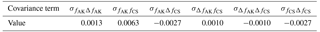
Table 2Covariances between terms for snow depth uncertainty calculation.

Download Print Version | Download XLSX

A secondary limitation of the methodology is the extent of the OIB campaigns; since they only operate in the western Arctic Ocean, north of the CAA, and in the Lincoln and Beaufort seas, no observations from the eastern Arctic go into our calibrations. Thus, the calibration functions derived are unconstrained outside of this area and we have less confidence in the snow depths in the eastern Arctic. Further, the calibration relationships are only strictly valid in spring, when OIB operates, so caution is warranted in using these products for seasonal variability of snow depth analysis.

3.2 Uncertainty calculation

The uncertainty calculation performed in this section assumes that the OIB products used in the analysis contain no systematic bias. We expect random noise to be minimised by grid averaging, but any systematic error would offset the calibration linear regression fits and alter snow depth retrievals. As discussed in Sect. 2.4, the recent study by Kwok et al. (2017) highlights the differences that exist between OIB snow radar data processed using various existing algorithms. It is not within the scope of this study to assess the sensitivity of our DuST product to the different OIB snow radar input data, but it remains the subject of future work. One purpose of the Kwok et al. (2017) inter-comparison was to identify the strengths and weaknesses of each processing technique in order to inform the design of an optimised algorithm and generate an improved snow radar product. We acknowledge that our methodology would benefit from such an effort and suggest that for future applications of this methodology – in particular to CS-2 and ICESat-2 – the next-generation of OIB snow depths should be investigated.

The equation for calculating snow depth, h_s, by our methodology is

where f_AK and f_CS are the AltiKa and CS-2 freeboards, and Δf_AK and Δf_CS are the AltiKa and CS-2 freeboard corrections (see Sect. 2.5 and 2.6). From propagation of errors on Eq. (2), the uncertainty on snow depth, ${\mathit{\sigma }}_{h_{\text{s}}}$, is given by

where the first four terms are the errors on the four variables in Eq. (2), and the last six terms are the covariances between them.

We obtain values of ${\mathit{\sigma }}_{f_{\text{AK}}}=\mathrm{9.4}$ cm and ${\mathit{\sigma }}_{f_{\text{CS}}}=\mathrm{8.4}$ cm from the 68 % prediction intervals on the calibration fits, represented by the shaded areas in Figs. 1 and 2 respectively.

Since our snow product is monthly gridded we are interested in monthly gridded snow depth uncertainty. Therefore ${\mathit{\sigma }}_{f_{\text{AK}}}$ and ${\mathit{\sigma }}_{f_{\text{CS}}}$ are the errors on the monthly gridded satellite freeboards to which the calibration corrections are being applied. According to Tilling et al. (2018), the error on the monthly gridded CS-2 freeboard is dominated by the uncertainty on the interpolated sea level anomaly (SLA), calculated from the SLAs of waveforms identified as leads (see Sect. 2.3). Lead SLAs within a 200 km along-track window centred on each floe measurement are fit with a linear regression to estimate the SLA beneath the floe and thus calculate the freeboard. As such, along-track floe measurements are not decorrelated at length scales less than 200 km, and the interpolated SLA uncertainty is not reduced from grid-cell averaging of data from the same satellite pass. Since the interpolation is performed along-track, separate satellite passes over each grid cell over the month are decorrelated, and thus the error is minimised by $\mathrm{1}/\sqrt{N}$, where N is the number of passes over a grid cell in 1 month. To calculate this error we reprocessed 1 month (January 2016) of CS-2 and AltiKa data, recording for each floe freeboard retrieval the 68 % prediction interval on the linear regression fit across the 200 km window. These errors, averaged on our 1.5^∘ longitude by 0.5^∘ latitude grid are shown in Fig. 6a. Since this error decorrelates from one satellite pass to the next, we divide by the number of satellite passes in a month (Fig. 6b) to retrieve the final interpolated SLA uncertainty, shown in Fig. 6c. Since this error dominates the freeboard retrieval (Tilling et al., 2018), this approximates to the monthly uncertainty on AltiKa and CS-2 freeboards, ${\mathit{\sigma }}_{f_{\text{AK}}}$ and ${\mathit{\sigma }}_{f_{\text{CS}}}$.

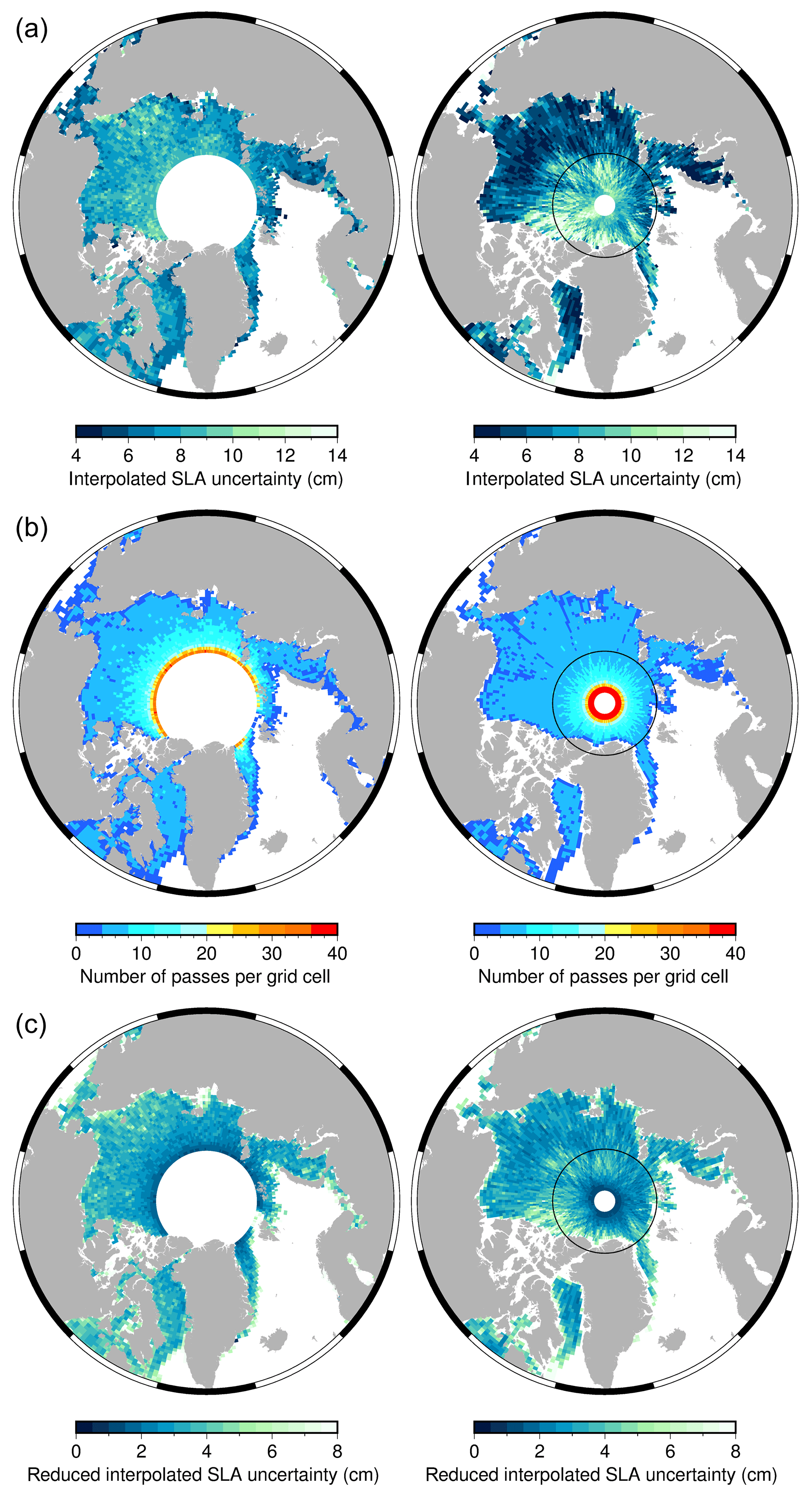
Figure 6Satellite freeboard error calculation for January 2016 for AltiKa (left) and CS-2 (right). (a) Monthly gridded sea level anomaly (SLA) error. (b) Number of tracks per (1.5^∘ long × 0.5^∘ lat) grid cell per month. (c) SLA error divided by the square root of the number of tracks, i.e. $\text{(a)}/\sqrt{\text{(b)}}$ gives the reduced monthly error on freeboard. The black circle on the CS-2 maps shows the upper latitude limit of DuST (81.5^∘ N).

Download

The last six terms of Eq. (3) are the covariances of the four variables. We calculate these by gridding all AltiKa and CS-2 data from March 2013 to January 2018 and finding the correlation–covariance matrix. The value for each term is summarised in Table 2.

All terms are substituted into Eq. (3) to find the uncertainty ${\mathit{\sigma }}_{h_{\text{s}}}$ on monthly gridded snow depth, shown for January 2016 in Fig. 7. The uncertainty is higher at lower latitudes where there are less satellite passes per grid cell, and over the thick multi-year ice to the north of the CAA where fewer leads available for the linear regression increase the uncertainty on the interpolated SLA, particularly for CS-2 (see Fig. 6a). As a conservative estimate we assign our monthly gridded snow depth product an average uncertainty of 8 cm for all months.

Figure 7January 2016 snow depth uncertainty.

Download

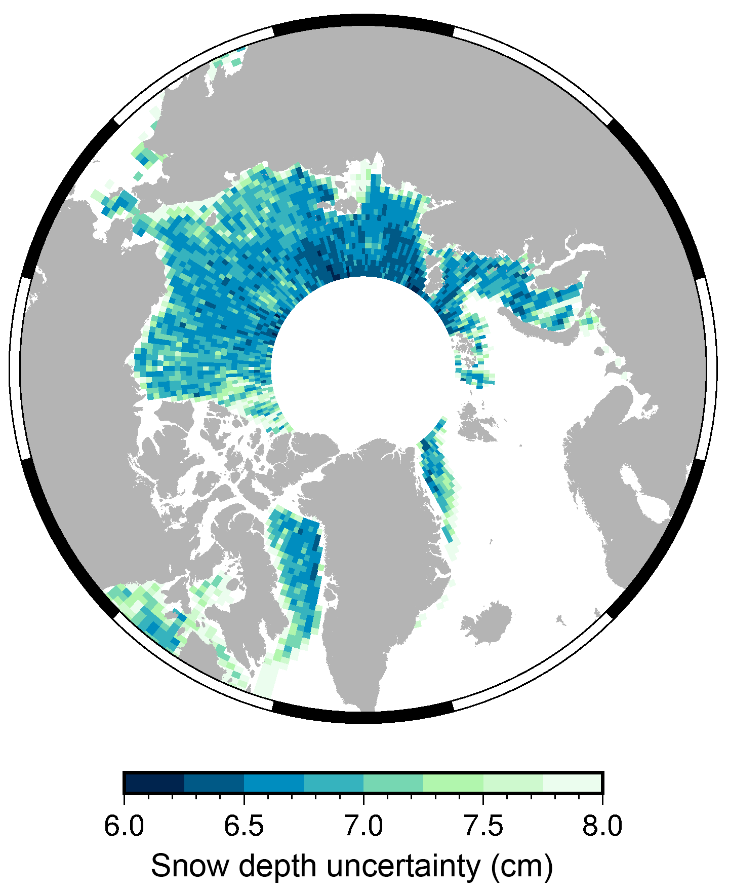
The main contribution to snow depth uncertainty is the prediction intervals from the calibration functions (see Sect. 2.5 and 2.6). This uncertainty could be reduced with the addition of more data points, i.e. more seasons of coincident satellite and OIB measurements. At time of publication OIB data for springs 2017 and 2018 have not been made publicly available.

3.3 Comparison with Operation IceBridge

We compare snow depth retrieved by our methodology with OIB snow depths from spring 2016 following the same procedure outlined in Sect. 2.5 and 2.6. For each day of the 2016 campaign, OIB snow depths are averaged onto the 2^∘ longitude × 0.5^∘ latitude grid, and grid cells containing less than 50 individual points are discarded to remove speckle noise, as before. Calibrated AltiKa and CS-2 freeboards for the ±10 days surrounding the campaign day are averaged onto the same grid and grid cells with less than 50 AltiKa or CS-2 points are discarded. The gridded, calibrated CS-2 freeboard is subtracted from the gridded calibrated AltiKa freeboard and multiplied by factor $c_{\text{s}}/c=\mathrm{0.781}$, as done previously. The resulting snow depth grid is then interpolated at the average position of the OIB data within each valid OIB grid cell. The DuST retrieved for each point is plotted against OIB snow depth.

In order to compare with more than one OIB campaign, we repeated the original calibration analyses outlined in Sect. 2.6 and 2.5, successively omitting each of the 2013–2015 OIB seasons and using the other 3 years' data to derive calibration functions and generate snow depths for the omitted year. DuST snow depths were then compared against OIB snow depths by the method outlined in the previous paragraph. Results for all 4 years are shown in Fig. 8 and summarised in Table 3.

Since OIB data were used to calibrate the satellite freeboards, this cannot be considered a validation exercise. However, if OIB is considered as providing true snow depth estimates (see discussion in Sect. 2.4 and 3.2), then the results suggest the ability to use the derived calibration relationships to predict snow depth when OIB does not operate, e.g. in future. The poor agreement between DuST and OIB for 2013 as compared to subsequent years could relate to the persistence and treatment of radar side lobes in the 2013 data (Kwok et al., 2017). Our analysis would benefit from the inclusion of additional OIB campaign data in the calibration and comparison. At present, OIB data for 2017 and 2018 are not available.

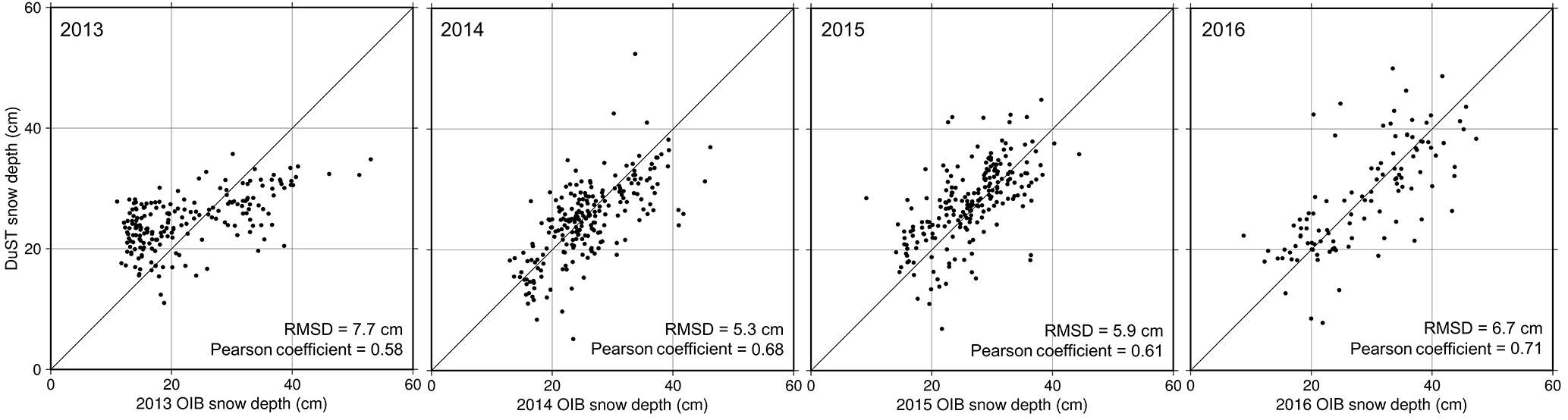
Figure 8Comparison of DuST and OIB snow depths for the 2013, 2014, 2015, and 2016 spring campaigns. Statistical results for all years are summarised in Table 3.

Download

Table 3Results of OIB and DuST comparison for the years 2013–2016.

Download Print Version | Download XLSX

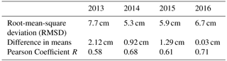
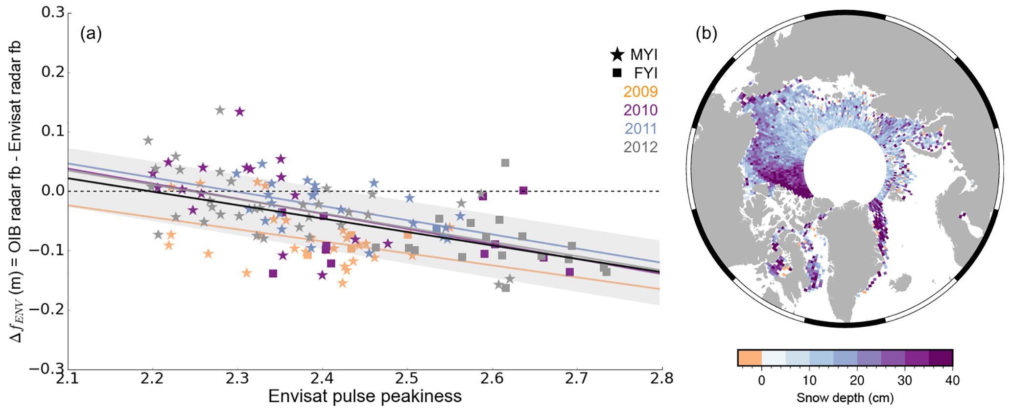
Figure 9(a) Envisat calibration relationship, derived from comparison of coincident OIB and Envisat data. Data and corresponding linear regression fits for 2009, 2010, 2011, and 2012 are shown in orange, purple, blue, and grey respectively. Star and square symbols represent multi-year and seasonal ice respectively, and the horizontal grey dashed line shows zero. (b) Snow depth for ICESat's 3E laser period (22 February–27 March 2006), retrieved by subtracting the calibrated Envisat freeboard from the ICESat freeboard and multiplying by a factor of 0.781. Please note that fb is freeboard.

Download

3.4 Application of DuST to ICESat-Envisat

The methodology outlined above demonstrates the ability to calibrate satellite freeboards with an independent data set in order to derive snow depth. It can be applied to any two coincident freeboard data sets and could be applicable to ICESat-2 which launched in September this year. In view of this possibility, we applied the methodology to the ICESat and Envisat satellites, whose periods of operation overlapped between 2003 and 2009.

The Radar Altimeter 2 (RA2) instrument operated on the Envisat satellite from 2002 until 2012. It was a pulse-limited Ku-band radar altimeter which like that aboard CS-2, operated at a central frequency of 13.575 GHz. NASA's ICESat mission featured a Geoscience Laser Altimeter System (GLAS) in order to accurately measure changes in the elevation of the Antarctic and Greenland ice sheets. This laser was also used to estimate ice thickness from laser freeboard retrieval (Kwok et al., 2007). Between 2003 and 2009, ICESat completed 17 observational campaigns; once every spring (February–March) and autumn (October–November) as well as three in the summers of 2004, 2005, and 2006.

ICESat had a 70 m diameter footprint, so we assume that biases due to footprint size or retracking method are negligible, and that it offers accurate estimates of the snow freeboard. We use available ICESat freeboard data (version 1) from NSIDC (Yi and Zwally, 2009), in our analysis. Envisat freeboard data were processed by CPOM, and the reader is referred to Ridout and Ivanova (2013) for further details on the algorithm.

Following the procedure outlined in Sect. 2.5, Envisat freeboard is calibrated to the snow–ice interface. Envisat has a larger footprint than AltiKa, nominally 2–10 km in diameter (Connor et al., 2009). As such, the waveform returns are more often classified as ambiguous (showing a complex mixture of scattering behaviour) and discarded, as discussed with reference to AltiKa in Sect. 2.3. As a result, Envisat data are sparsely populated and in order to have sufficient coverage for comparison with OIB data as well as 50 or more points per grid cell (to reduce speckle noise), it was necessary to increase both the grid resolution and time window as compared with the calibration procedure performed for AltiKa and CS-2.

Satellite data for the ±15 days surrounding each 2009–2012 OIB campaign day were averaged onto a 3^∘ longitude × 0.75^∘ latitude grid. The value Δf_ENV, defined as the OIB radar freeboard minus the Envisat freeboard and plotted against Envisat PP, is shown in Fig. 9a. The combined (all years) linear regression fit is shown by the black line and has slope of −0.23 and intercept 0.50. The shaded area shows the 68 % prediction interval for the CLRF, corresponding to a ±5 cm standard error on Δf_ENV.

Dual-altimeter snow thickness, retrieved by subtracting the calibrated Envisat freeboard from the ICESat freeboard, is shown in Fig. 9b for the ICESat laser period 3E (22 February–27 March 2006). Snow depth spatial distribution follows the expected pattern of thicker snow (30–40 cm) over multi-year ice to the north of the Canadian Archipelago and in the Fram Strait, and thinner snow cover (<20 cm) over seasonal ice. Overall higher magnitudes as compared with March 2016 (Fig. 3) could be the result of a decline in multi-year ice fraction and precipitation over the past decade. Though validation is required, the result demonstrates the viability of combining laser and calibrated radar freeboards to retrieve snow depth.