the Creative Commons Attribution 4.0 License.
the Creative Commons Attribution 4.0 License.
 | 22 Nov 2018
Neutral equilibrium and forcing feedbacks in marine ice sheet modelling
Rupert M. Gladstone
Yuwei Xia
John Moore
Poor convergence with resolution of ice sheet models when simulating grounding line migration has been known about for over a decade. However, some of the associated numerical artefacts remain absent from the published literature.
In the current study we apply a Stokes-flow finite-element marine ice sheet model to idealised grounding line evolution experiments. We show that with insufficiently fine model resolution, a region containing multiple steady-state grounding line positions exists, with one steady state per node of the model mesh. This has important implications for the design of perturbation experiments used to test convergence of grounding line behaviour with resolution. Specifically, the design of perturbation experiments can be under-constrained, potentially leading to a “false positive” result. In this context a false positive is an experiment that appears to achieve convergence when in fact the model configuration is not close to its converged state. We demonstrate a false positive: an apparently successful perturbation experiment (i.e. reversibility is shown) for a model configuration that is not close to a converged solution. If perturbation experiments are to be used in the future, experiment design should be modified to provide additional constraints to the initialisation and spin-up requirements.
This region of multiple locally stable steady-state grounding line positions has previously been mistakenly described as neutral equilibrium. This distinction has important implications for understanding the impacts of discretising a forcing feedback involving grounding line position and basal friction. This forcing feedback cannot, in general, exist in a region of neutral equilibrium and could be the main cause of poor convergence in grounding line modelling.


Strongly resolution-dependent behaviour when implementing grounding line movement (sometimes referred to as grounding line migration) in a marine ice sheet model was identified by Vieli and Payne (2005) and was further characterised as a convergence problem by subsequent studies (Durand et al., 2009; Gladstone et al., 2010a, b, 2012; Goldberg et al., 2009). In the current study “convergence” refers to the approach of model outputs to a consistent state as resolution is made progressively finer. Some models incorporating a moving grid that explicitly tracks grounding line position do not appear to exhibit this poor convergence (Vieli and Payne, 2005). Various forms of mesh refinement help to address the problem, though very high resolution is still needed (Cornford et al., 2013; Goldberg et al., 2009), and special treatments of the grid cell or element containing the grounding line can also improve convergence (Feldmann et al., 2014; Gagliardini et al., 2016; Gladstone et al., 2010b; Pollard and DeConto, 2009; Seroussi et al., 2014).
This problem has also been described as neutral equilibrium (Durand et al., 2009; Pattyn et al., 2006) in modelling studies. This terminology may follow from earlier studies in which it was proposed that real marine ice sheet systems may exhibit neutral equilibrium (Hindmarsh, 2006). Although these theories are no longer accepted (Schoof, 2007), un-converged model behaviour at coarse resolution is still sometimes referred to as neutral equilibrium (Durand et al., 2009).
Most of the studies cited above use a Weertman sliding relation (Weertman, 1957). More recent studies (Gladstone et al., 2017; Leguy et al., 2014; Tsai et al., 2015) suggest that the convergence issues may be to some extent mitigated by use of sliding relations incorporating a dependence on effective pressure at the bed. However, irrespective of sliding law, similar convergence issues may arise due to a step change in basal melting at the grounding line (Gladstone et al., 2017). The numerical implementation of basal melting at the element or grid cell scale may also have a large impact on convergence (Seroussi and Morlighem, 2018).
In the current study we employ a flow line Stokes-flow model with Weertman sliding and no basal melting (Sect. 2) to further characterise the nature of this grounding line convergence issue (Sect. 3). We choose a set-up in which the problem is under-resolved; i.e. the model outputs are not close to a converged solution. This is chosen in order to demonstrate the nature of the numerical artefacts arising at coarse resolution. We explore implications for design of computer experiments (Sect. 3.1) and for the issue of neutral equilibrium (Sect. 4). This leads to a discussion on discretisation of a forcing feedback involving basal friction and model state (Sect. 5).
Our aim is to provide a model configuration in which convergence with resolution is not achieved (i.e. our resolution is too coarse for self-consistent model behaviour), and explore the nature of the grounding line problems. Our set-up is similar to that of the original Marine Ice Sheet Model Intercomparison Project (Pattyn et al., 2012), with a linear bed, Weertman sliding, and spatially uniform surface accumulation.
We use the ice dynamic model (IDM) Elmer/Ice (Gagliardini et al., 2013). The Stokes equations for a viscous fluid with non-linear rheology are solved using the finite-element method over a two-dimensional flow line domain (one vertical and one horizontal dimension) with grounding line capability.
A contact problem is solved to determine the evolving grounding line position (Favier et al., 2012), which is constrained to be located at a node. Basal resistance, or friction, in the vicinity of the grounding line is determined using the discontinuous approach (DI in Gagliardini et al., 2016). This imposes full friction for all grounded elements and free slip for all floating elements, with the element containing both grounded and floating nodes considered to be floating.
The rheology follows Glen's law (Glen, 1952; Paterson, 1994) with viscosity calculated using a temperature-dependent Arrhenius law (Gagliardini et al., 2013; Paterson, 1994). A constant uniform temperature of −15 ∘C is used in all simulations.
The linear downsloping bedrock, b, is given in metres relative to sea level by
where x is distance from the inland boundary. The domain length is 600 km.
The horizontal component of the velocity is set to zero at the inland boundary, and an ocean pressure condition is applied at the ice front and under the floating ice shelf. We take ice density to be 910 kg m−3 and water density to be 1000 kg m−3.
A spatially uniform net surface accumulation flux, a, is used, and this value is varied between simulations.
The basal friction or shear stress, τb, acts opposite to the direction of flow and has the magnitude (Weertman, 1957)
where ub is the sliding velocity and C is a friction coefficient. C is set to 0.02417 MPa m−⅓ a⅓ for all simulations in the current study.
The simulations carried out for the current study are described below. They comprise grounding line advance simulations followed by grounding line retreat simulations (Sect. 2.1). In some cases further perturbation experiments are then carried out (Sect. 2.2). These simulations were all carried out with a horizontally uniform element size of 1 km and a time step size of 0.2 years. Typical steady-state profiles for this model set-up are shown in Fig. 1.
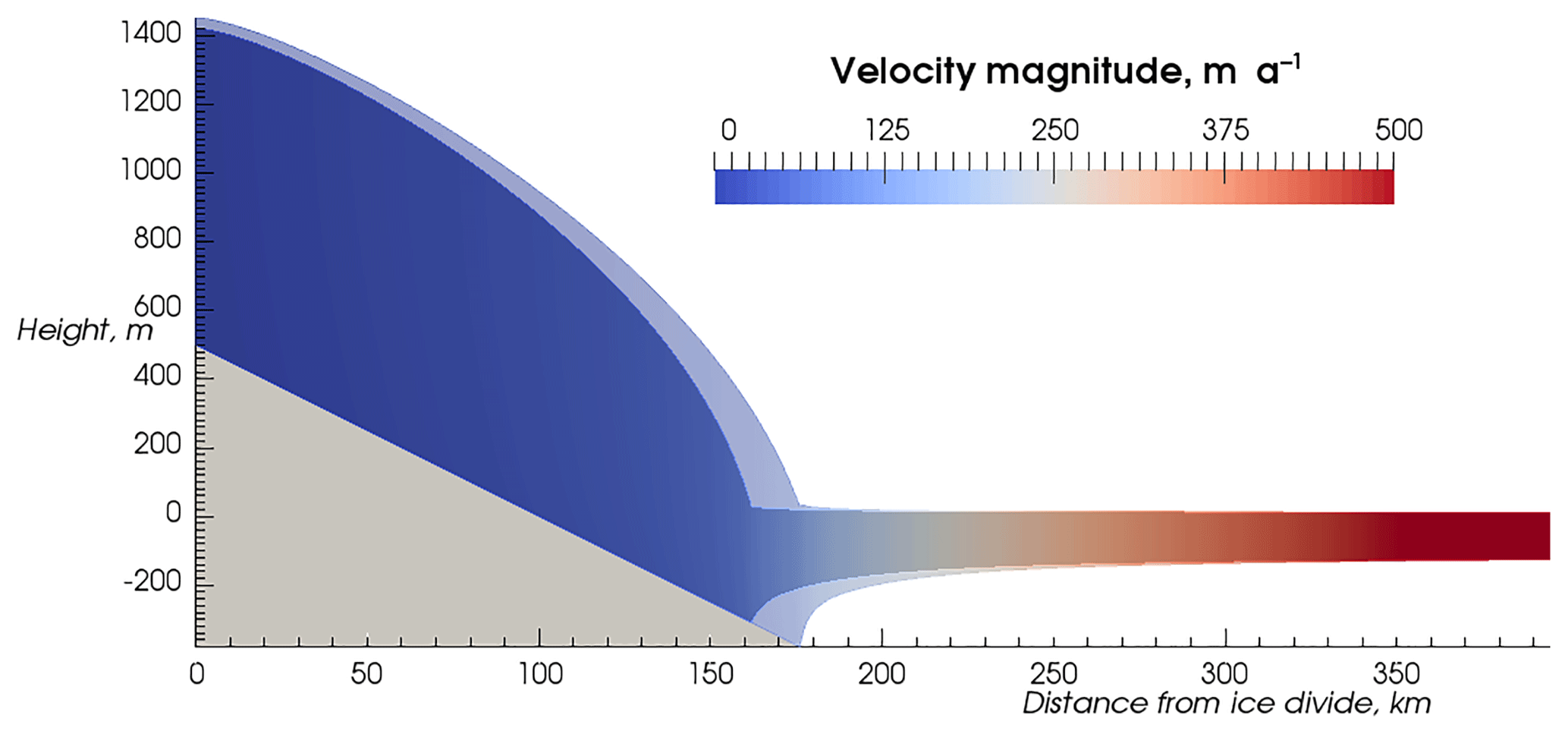
Figure 1Ice sheet profiles after 13 kyr at the end of the advance–retreat simulations described in Sect. 2.1. The simulations with an advance forcing of a=0.7 m a−1 (solid colour) and a=1.7 m a−1 (semi-transparent) are shown. These states provide the initial state for perturbation experiments P1 and P2 respectively (Sect. 2.2). Vertical exaggeration is 100 times.
2.1 Advance–retreat experiments
The advance simulations are spun up from a uniform slab of 100 m in thickness. They comprise 7 kyr of evolution with a different net accumulation forcing for each simulation. Values range from 0.2 to 2.0 m a−1 (the full set of values used is given in the Fig. 2 legend).
The advance simulations are followed immediately by ”retreat” simulations, which in some (but not all) cases exhibit grounding line retreat. These simulations continue from the final states of the advance simulations. They all use a net accumulation forcing of a=0.2 m a−1 and are run for a further 6 kyr.
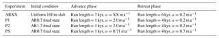
Each pair of advance and retreat simulations constitutes an ARXX experiment, for which XX indicates the accumulation forcing used for the advance phase (e.g. AR0.7 refers to the advance simulation with a=0.7 m a−1 and the corresponding retreat phase). Experiments are summarised in Table 1.
2.2 Perturbation experiments
Starting from the final states of two of the advance–retreat simulations, (i.e. after 13 kyr total simulation time) we carried out two perturbation simulations. P1 starts from the final state of experiment AR0.7 (which used an advance forcing of a=0.7 m a−1), and P2 starts from the final state of AR1.7. AR0.7 and AR1.7 are shown with a dotted line in Fig. 2 and their final states (which form the initial states for P1 and P2) are shown in Fig. 1. Note that although P1 and P2 start from approximate steady states, and in both cases the steady state was approached with a=0.2 m a−1, these steady states are distinct. The forcing for the perturbation experiments P1 and P2 is identical apart from initial state. They are run for 1 kyr with a=2.0 m a−1 followed by 4 kyr with a=0.2 m a−1. The perturbation experiments P1 and P2 are shown in Fig. 3.
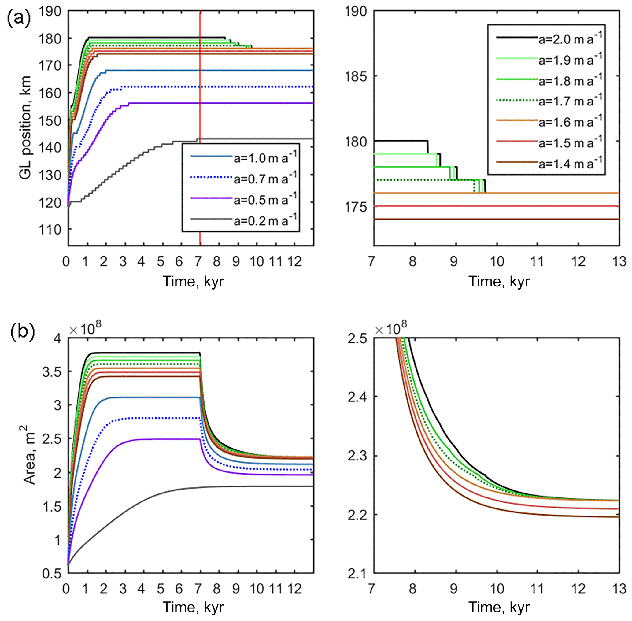
Figure 2Advance–retreat simulations (described in Sect. 2.1). Evolution of (a) grounding line position for all simulations and (b) ice area. Area in this case is the flow line equivalent of ice volume for a 3-D ice sheet and can also be interpreted as volume per unit width of the glacier. The right-hand subplots show details of a subset of the retreat simulations. The red vertical line indicates the forcing change at 7 kyr when the simulations switch from advance to retreat. The legend shows the accumulation rates prescribed during the advance phase, while for the retreat accumulation was 0.2 m a−1. The dotted lines are the cases also shown in Fig. 1 and provide the initial state for the P1 and P2 experiments (described in Sect. 2.2).
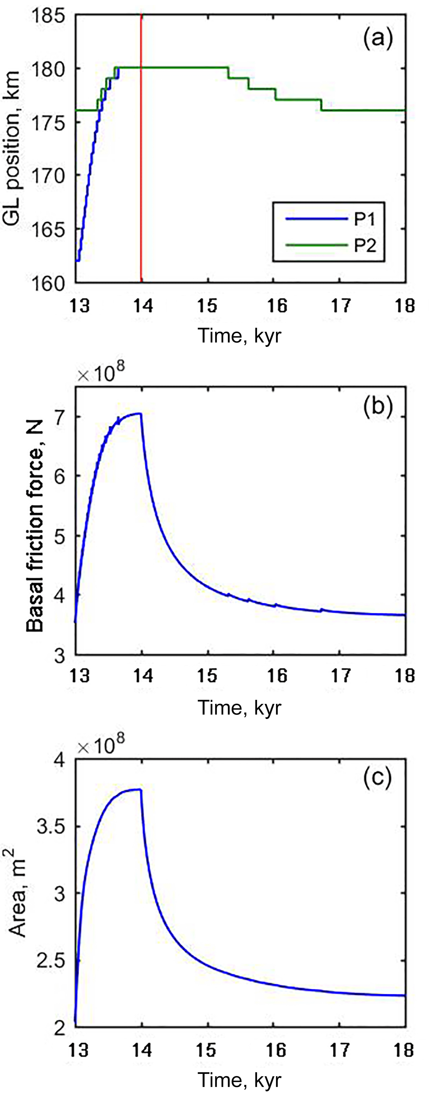
Figure 3Evolution of (a) grounding line position, (b) total basal friction (this is the basal shear stress integrated over the grounded region), and (c) ice area (the flow line equivalent of volume) for perturbation experiments. Both perturbation experiments P1 and P2 are shown in (a), and the difference in initial states is clearly visible. Panels (b) and (c) show only P1. Both P1 and P2 were run for 1 kyr with an accumulation rate a=2.0 m a−1 followed by 4 kyr with a=0.2 m a−1.
We also carried out a small perturbation experiment, PS. PS starts from the same state as P1. It is identical to P1 except that the magnitude of the perturbed forcing is a=0.71 m a−1 and the retreat phase has a=0.7 m a−1. Experiments are summarised in Table 1.
Figure 2 summarises the evolution over time of the advance–retreat simulations. Although a formal test for steady state was not imposed, we calculated the rate of change of area and found it to be of the order of 10−8 m2a−1 or smaller at the end of all advance simulations and all retreat simulations (except for AR0.2 for which we calculated the rate only at the end of the retreat simulation as it was not yet at steady state after 7 kyr). Given that 7 kyr is sufficient to approach steady state, retreat should occur after 7 kyr for all simulations in which a was initially greater than 0.2 m a−1. This is due to the uniqueness of stable ice sheet configurations on a linear downsloping bed, demonstrated for a “shelfy-stream” approximation by Schoof (2007). However, as also seen with a shelfy-stream model (Gladstone et al., 2010a), multiple steady states exist as a model artefact.
The multiple steady states that exist after 13 kyr are almost certainly numerical artefacts, with the underlying system having only one viable steady state. Similar studies have shown that the size of this region decreases with finer resolution (Gladstone et al., 2010a). The region containing steady-state grounding line positions (at the end of the retreat phase) in the current study spans from x=143 km to x=176 km. We propose that the model is capable of exhibiting as many viable steady-state grounding line positions as there are mesh nodes within this region. We tested this hypothesis near the seaward end of the region by implementing small increments in a between advance simulations (experiments AR1.4 up to AR2.0). Specifically we obtained a final grounding line position on every node from x=174 km to x=180 km for the advance simulations and from x=174 km to x=176 km for the retreat simulations (Fig. 2, upper right panel).
The volume evolution plots indicate a reduction in volume for all retreat simulations (except the simulation which advanced under a=0.2 m a−1 forcing), even for simulations showing no grounding line movement (experiments AR0.2 up to AR1.6). Simulations ending the retreat phase with the same grounding line position (experiments AR1.6 up to AR2.0 end at 176 km) have the same final volume. Simulations with a more landward final grounding line position have a lower final volume. Thus, for our set-up, 176 km marks the seaward end of the region of steady-state grounding line positions under a forcing of a=0.2 m a−1. Our explanation for this numerical artefact involves discretisation of a feedback between model state (especially grounding line position) and total basal resistance, which we discuss in Sect. 5.
3.1 Implications for experiment design
Here we consider perturbation experiments P1 and P2, both of which adhere to a typical perturbation design and both of which experience identical forcing during the experiment. Perturbation experiments are common in IDM studies and intercomparison projects (e.g. Favier et al., 2012; Pattyn et al., 2006, 2012, 2013). The premise is that an initial spin-up procedure results in an IDM in steady state. A forcing perturbation is applied, causing change, and then removed. The analysis then considers whether or not reversibility has been demonstrated (i.e. whether the IDM state returned to its post spin-up state after the forcing perturbation was reset). However, the existence of multiple steady-state grounding line positions means that the requirement to start in steady state is not sufficient to constrain the initial (post-spin-up) state.
The outputs of the perturbation experiments are shown in Fig. 3. Although both experiments adhere to typical perturbation experiment design, and are both subject to the same perturbation, P2 shows full reversibility (in all aspects of model state, including grounding line position, ice volume, and total friction) and P1 does not. The outcomes in terms of reversibility are opposites, resulting directly from the choice of initial state. Here, P2 is a false positive because considered in isolation it would appear to indicate a converged result, but convergence has not been achieved. In general a converged experiment (i.e. with sufficiently fine resolution to achieve a self consistent result) will always demonstrate reversibility on a linear bed (Schoof, 2007), but our results demonstrate that reversibility is not in itself a sufficient criterion to establish convergence.
We now consider an example of this vulnerability in design of perturbation experiments from the published literature. Pattyn et al. (2006) investigated the role of transition zones in grounding line modelling. The transition zone is a region immediately upstream of the grounding line over which the stress state changes from a grounded regime (in which high basal shear stress approximately balances gravitational driving stress) to a floating regime (in which basal shear stress is zero and longitudinal stress in the ice balances a low gravitational driving stress).
Pattyn et al. (2006) used a spin-up procedure that resulted, for most of their simulations, in retreat of the grounding line as steady state was approached. This suggests (but does not prove) that the end of the spin-up resulted in a steady-state grounding line position located at the seaward end of the region of multiple steady states, analogous to our experiment P2 (Fig. 3). These simulations did demonstrate reversibility. However, their simulation with a short prescribed grounding line transition zone involved no movement of the grounding line as steady state was approached. This suggests (but again does not prove) that the end of the spin-up resulted in a steady-state grounding line position somewhere within the region of multiple steady states, analogous to our experiment P1 (Fig. 3); see Fig. 4 of Pattyn et al. (2006). This simulation did not demonstrate reversibility. Thus the result of Pattyn et al. (2006) that a longer transition zone results in better reversibility may be an artefact of their experiment design rather than a robust result.
3.2 Initialisation through inversion
A common method for initialisation of IDMs is to infer basal properties and ice viscosity (or temperature) through inverse techniques, steady-state temperature simulations, and surface relaxation (Cornford et al., 2015; Gillet-Chaulet et al., 2012, 2016; Gladstone et al., 2014; Morlighem et al., 2010; Zhao et al., 2018). These methods can lead to an initial state that is close to steady state, but without any information as to whether convergence is achieved, and hence whether multiple steady states may exist. If a transient simulation intialised in such a way leads to little or no change in terms of grounding line position, it cannot be concluded that the real system being modelled is close to steady state because the possibility remains that the modelled steady state is a result of under-resolution.
If a convergence study is carried out for the system undergoing retreat, for example if high basal melt forcing is applied (Favier et al., 2014), this does not prove that the model will also exhibit converged behaviour in advance, nor even does it prove that regions of stationary grounding line within the domain are indicative of a converged result. Conversely, convergence of advance behaviour does not prove convergence of retreat behaviour. The current study does not fully explore the implications of multiple steady grounding line positions in 3-D real world cases, which is especially complicated in that some regions may exhibit an advancing grounding line while others exhibit a retreating grounding line. Based on current simulations the authors recommend that both advance and retreat convergence tests be carried out in order to have full confidence in modelled behaviour.
An equilibrium state (or steady state) of a system is a state that does not change unless the forcing changes. In the context of IDM grounding line simulations, this means that neither the forcing applied to the domain nor the ice sheet configuration change over time. Such steady states are typically obtained through long simulations in which forcing is kept constant and the state of the simulated ice sheet gradually stops evolving as equilibrium is approached.
It is important to clarify different types of equilibria for the following discussion. Consider the example of a ball at rest (i.e. in equilibrium) under gravitation on a solid surface. The ball is then subjected to a perturbation: it is moved along the surface then left only under gravitation. Different types of equilibrium may be illustrated by considering the behaviour of the ball after the perturbation has been removed.
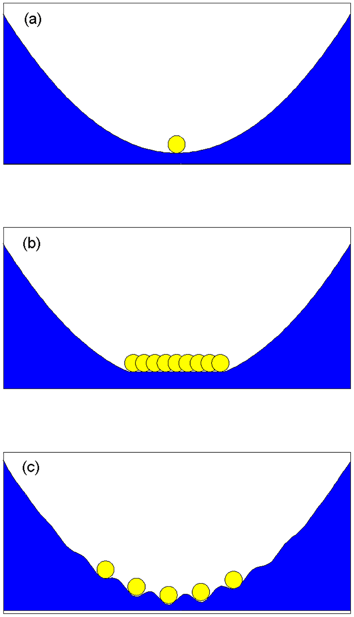
Figure 4A simple idealised system of a ball under gravitation used to demonstrate types of equilibria: (a) one stable equilibrium is present and the ball will always tend to return to this; (b) a region of neutral equilibrium is present (a region of flat surface), and the ball will remain in equilibrium anywhere on this surface; (c) multiple locally stable equilibria exist, and the ball will tend to roll downhill to the nearest.
An equilibrium state in which the perturbation results in the system tending to return to the original state is a stable equilibrium (e.g. Fig. 4a – the ball rolls back down to the original position).
An equilibrium state in which the perturbation results in the system tending to move further from the original state is an unstable equilibrium (not shown, but consider a ball perched on the summit of a hill – it will continue rolling away from the summit after being given a small push in any direction).
An equilibrium state in which the perturbation results in the system remaining in the new state is termed neutral equilibrium (e.g. Fig. 4b – the ball may be at rest anywhere on the flat region).
Figure 4c illustrates a system with multiple locally stable equilibria within a confined region. A sufficiently large perturbation will result in the ball finding a new equilibrium position, but a small perturbation will result in a return to the original position.
These types of behaviour for a ball under gravity have analogies for a marine ice sheet system. Schoof (2007) demonstrated the existence of a single stable equilibrium for a marine ice sheet on a downward-sloping (in the ice flow direction) bed. Schoof (2007) also demonstrated the existence of an unstable equilibrium on an upward-sloping bed, though this may not always be the case in the presence of high lateral drag (Gudmundsson et al., 2012; Katz and Worster, 2010). As mentioned in Sect. 1, neutral equilibrium in real world marine ice sheet systems is no longer considered plausible, but multiple stable equilibria could exist as a function of bedrock geometry (Schoof, 2007).
IDM studies using different models have demonstrated that multiple steady states can, as a numerical artefact, exist in models in which the system being modelled should exhibit a single stable equilibrium (Durand et al., 2009; Gladstone et al., 2010a). This has been referred to as neutral equilibrium (Durand et al., 2009), and here we consider the distinction between a region of neutral equilibrium and a region of multiple locally stable steady states. We argue that IDMs exhibit, as a numerical artefact, a region containing multiple locally stable equilibria (similar to Fig. 4c) and not a region of neutral equilibrium.
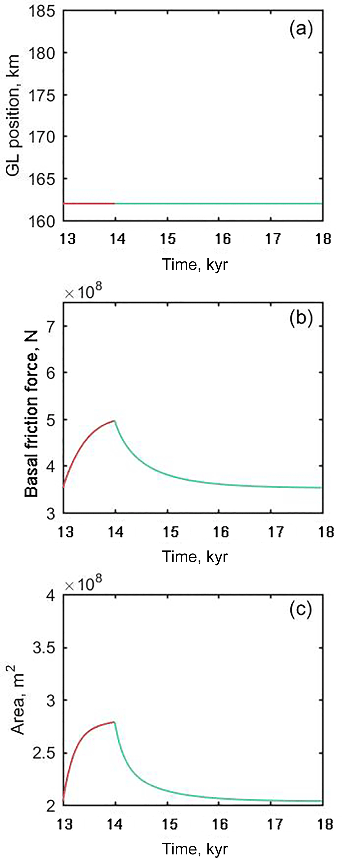
Figure 5Evolution of (a) grounding line position, (b) total basal friction, and (c) ice area (the flow line equivalent of volume) for the small perturbation experiment PS. PS is identical to P1 except that the magnitude of the perturbed forcing for the first 1 kyr is a=0.71 m a−1 and for the last 4 kyr is a=0.7 m a−1.
Figure 5 shows output from experiment PS, the small perturbation experiment. The perturbation, although not sufficient to cause a change in grounding line position (Fig. 5a), is sufficient to cause a shift in model state, as evidenced by the change in total ice volume (Fig. 5c). However, the forcing reset results in a return to the original state. This behaviour indicates a locally stable steady state rather than a region of neutral equilibrium. This argument against marine IDMs exhibiting neutral equilibria may appear to be a matter of semantics, but there are important implications toward understanding the nature of the grounding line convergence problem, discussed in Sect. 5.
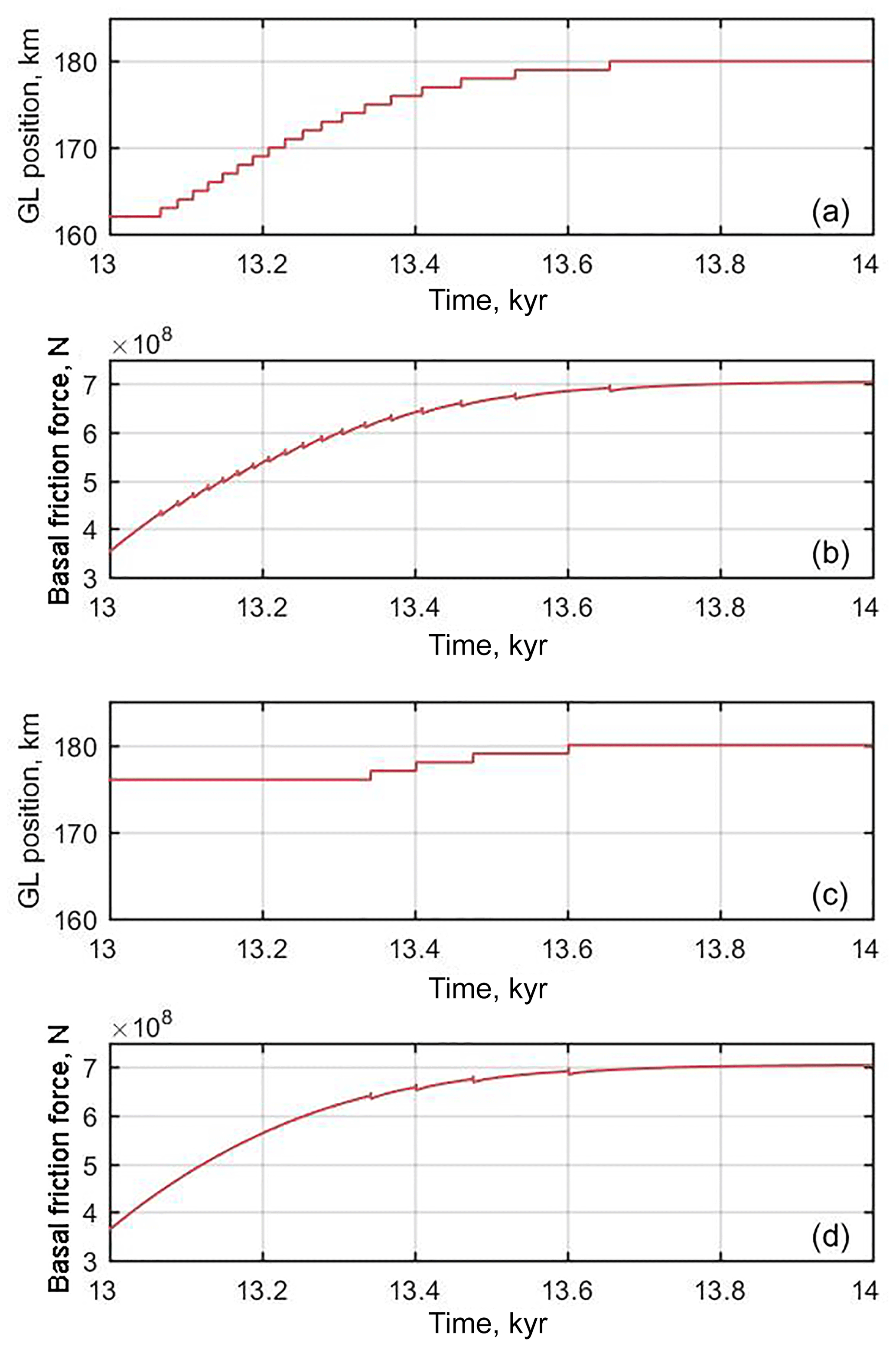
Figure 6A closer look at the advance phase of the perturbation experiments. Evolution of (a) grounding line position for P1, (b) total basal friction for P1, (c) grounding line position for P2, and (d) total basal friction for P2.
Figure 6 shows, in more detail, the evolution of total basal friction during the advance phase of perturbation experiments P1 and P2. The spikes in total friction correspond to advance of the grounding line by a single element. These features are characterised by an instantaneous increase in total friction followed by a rapid decrease and an ensuing gradual increase. The spikes can be explained as follows: An instantaneous increase in basal friction results from a grounding line advance due to the increased contact area. This increase reduces the sliding velocity, causing the rapid decrease in total friction. This is followed by a more gradual return to the longer-term trend.
This is a model discretisation of what should be a continuous feedback: incremental grounding line advance should cause incremental increase in total basal friction, causing an incremental slowing and thickening. This positive feedback (which we refer to as the friction force feedback) between grounded extent and total friction is continuous in the underlying system being simulated but heavily discretised in the model due to basal friction reaching a peak at the grounding line. The modelled flux across the grounding line must be higher than that of the system it attempts to represent in order to compensate for the missing basal friction immediately downstream of the grounding line due to the discretisation. Specifically, the PS experiment (Fig. 5) demonstrates that even an increase in modelled volume and total friction force of several tens of percent may not be sufficient to cause a single element of grounding line advance. This understanding could not have been attained if the region of multiple locally stable steady states was viewed as a region of neutral equilibrium because a neutral equilibrium can have no positive feedback between forcing and state (except in the vanishingly low probability case of an exactly compensating mechanism).
We postulate that this discretisation of a continuous feedback is the main cause of numerical artefacts and poor convergence with resolution in grounding line modelling. This is consistent with the finding that sliding relations incorporating a strong dependency on effective pressure at the bed show far better convergence with resolution (Gladstone et al., 2017). This is due to the basal friction approaching zero at the grounding line, so that the advance or retreat of the grounding line by a single element will not have a significant impact on total basal friction.
Considering several published sliding relations that feature a dependence on effective pressure, it should be noted that the hybrid sliding relations of Gagliardini et al. (2007) and Tsai et al. (2015) typically feature steep basal friction gradients over a transition zone near the grounding line (Brondex et al., 2017) and so may not exhibit such good convergence as the sliding relation of Budd et al. (1979, 1984). It should also be noted that improved convergence is not a valid reason to choose one sliding relation over another: physical realism should be the deciding factor. A final note is that this issue is not fundamentally specific to the equations solved for ice flow, so while the simulations carried out here use Elmer/Ice to solve the Stokes equations, the same principles should apply in other IDMs that implement some kind of sliding relation.
It might be thought that a special treatment of the grid cell or element containing the grounding line, such that the grounding line position within the cell or element can be represented, would resolve this problem of discretising the friction force feedback. However, the grounding line parameterisations introduced by Gladstone et al. (2010b) (a study featuring numerous different parameterisations implemented in a flow line shelfy-stream model) still show a strong non-linear behaviour correlated to grid cell grounding line advance in the evolution of model state (see Gladstone et al., 2010b, Figs. 3, 4, and 6). Gladstone et al. (2010b) also find that multiple steady states exist, with one steady-state grounding line position per grid cell, although the steady-state position is not constrained to lie on a grid point. Thus grounding line parameterisations do not necessarily resolve the problem of a discretised (or highly non-linear on a grid cell scale) friction forcing feedback.
The poor convergence of IDMs regarding grounding line movement emphasises the important, and hopefully obvious, requirement that all IDM studies featuring grounding line movement demonstrate that sufficiently fine resolution has been used to achieve a converged result. The resolution must be such that the region of multiple steady states, which is known to be a numerical artefact, must collapse toward zero (we suggest as a rule of thumb that it be required to be no larger than one grid cell or element, though this is not itself a formal demonstration of convergence). Reversibility experiments cannot in general demonstrate that sufficiently fine resolution has been achieved.
Basal melting
As mentioned above, the forcing feedback involving total basal resistance will be of greatly reduced magnitude in the case of sliding relations in which the basal resistance smoothly transitions to zero approaching the grounding line. Given the currently increasing use of such sliding relations (Brondex et al., 2017; Gladstone et al., 2017; Tsai et al., 2015), it might seem that the impacts on experiment design described here (Sect. 3.1) will not be widely applicable. However, recent studies have shown that ocean-induced melting at the base of ice shelves can cause convergence problems, both at a sub-grid scale (Seroussi and Morlighem, 2018) and over multiple grid cells or elements (Gladstone et al., 2017). Given that these convergence problems can be partially mitigated by smoothing the basal melt to approach zero approaching the grounding line (in this case approaching from seaward rather than landward), we propose that a forcing feedback, analogous to the friction force feedback, is involved. In this case it is between basal melting and geometry: a retreating grounding line will expose more basal area to melting, increasing thinning in the vicinity of the grounding line and enhancing retreat. Discretisation of this melt forcing feedback also leads to the existence of a region of multiple steady states at coarse resolution (Gladstone et al., 2017, Fig. 5), implying that the same restrictions on experiment design will apply.
The established poor convergence of many marine ice sheet models regarding grounding line movement is characterised by a region of multiple locally stable states. Our results demonstrate that this is not, as has been previously claimed, a neutral equilibrium.
This region of steady states implies that perturbation experiments, such as are often used in model intercomparison projects, can have a hitherto unrecognised dependence on initial conditions, potentially leading to false positives. Thus the size of the region of multiple locally stable steady states may be a more useful metric for assessing convergence of modelled grounding line movement than advance-only simulations, retreat-only simulations, or reversibility. Specifically, the region should reduce with finer resolution and should be vanishingly small at published resolutions. If perturbation experiments are used in future tests of convergence of grounding line behaviour, we advocate that the spin-up method must also be prescribed, as a simple requirement for steady state is not in general sufficient to constrain the experiment design.
This poor convergence is not only a result of inherent difficulties in representing a spatial step change in basal drag across the grounding line, but also due to a temporal forcing feedback involving grounding line movement and basal shear stress.
These results apply to marine ice sheet models using a Weertman sliding relation. The same qualitative features occur with sliding relations incorporating a smoother transition in basal drag across the grounding line, such as through a dependence on height above buoyancy, but with a smaller magnitude. A similar convergence issue is raised when imposing basal melt under the floating ice shelf.
The study is based on the computer code Elmer/Ice https://github.com/ElmerCSC/elmerfem/releases/tag/release-8.3 (last access: 24 May 2017).
RG designed the experiments and led the paper writing. YX carried out the simulations and contributed to the paper. JM contributed to interpretation of results and writing the paper.
The authors declare that they have no conflict of interest.
This research was supported by Academy of Finland grant number 286587.
The authors wish to acknowledge CSC – IT Centre for Science, Finland, for computational
resources.
Edited by: Alexander Robinson
Reviewed by: two anonymous referees
Brondex, J., Gagliardini, O., Gillet-Chaulet, F., and Durand, G.: Sensitivity of grounding line dynamics to the choice of the friction law, J. Glaciol., 63, 854–866, https://doi.org/10.1017/jog.2017.51, 2017. a, b
Budd, W., Keage, P. L., and Blundy, N. A.: Empirical studies of ice sliding, J. Glaciol., 23, 157–170, 1979. a
Budd, W., Jenssen, D., and Smith, I.: A 3-dimensional time-dependent model of the West Antarctic Ice-Sheet, Ann. Glaciol., 5, 29–36, https://doi.org/10.3189/1984AoG5-1-29-36, 1984. a
Cornford, S. L., Martin, D. F., Graves, D. T., Ranken, D. F., Le Brocq, A. M., Gladstone, R. M., Payne, A. J., Ng, E., and Lipscomb, W. H.: Adaptive mesh, finite volume modeling of marine ice sheets, J. Comput. Phys., 232, 529–549, https://doi.org/10.1016/j.jcp.2012.08.037, 2013. a
Cornford, S. L., Martin, D. F., Payne, A. J., Ng, E. G., Le Brocq, A. M., Gladstone, R. M., Edwards, T. L., Shannon, S. R., Agosta, C., van den Broeke, M. R., Hellmer, H. H., Krinner, G., Ligtenberg, S. R. M., Timmermann, R., and Vaughan, D. G.: Century-scale simulations of the response of the West Antarctic Ice Sheet to a warming climate, The Cryosphere, 9, 1579–1600, https://doi.org/10.5194/tc-9-1579-2015, 2015. a
Durand, G., Gagliardini, O., de Fleurian, B., Zwinger, T., and Le Meur, E.: Marine ice sheet dynamics: Hysteresis and neutral equilibrium, J. Geophys. Res.-Earth Surf., 114, F03009, https://doi.org/10.1029/2008JF001170, 2009. a, b, c, d, e
Favier, L., Gagliardini, O., Durand, G., and Zwinger, T.: A three-dimensional full Stokes model of the grounding line dynamics: effect of a pinning point beneath the ice shelf, The Cryosphere, 6, 101–112, https://doi.org/10.5194/tc-6-101-2012, 2012. a, b
Favier, L., Durand, G., Cornford, S. L., Gudmundsson, G. H., Gagliardini, O., Gillet-Chaulet, F., Zwinger, T., Payne, A. J., and Le Brocq, A. M.: Retreat of Pine Island Glacier controlled by marine ice-sheet instability, Nat. Clim. Change, 4, 117–121, https://doi.org/10.1038/NCLIMATE2094, 2014. a
Feldmann, J., Albrecht, T., Khroulev, C., Pattyn, F., and Levermann, A.: Resolution-dependent performance of grounding line motion in a shallow model compared to a full-Stokes model according to the MISMIP3d intercomparison, J. Glaciol., 60, 353–360, https://doi.org/10.3189/2014JoG13J093, 2014. a
Gagliardini, O., Cohen, D., Raback, P., and Zwinger, T.: Finite-element modeling of subglacial cavities and related friction law, J. Geophys. Res.-Earth Surf., 112, F02027, https://doi.org/10.1029/2006JF000576, 2007. a
Gagliardini, O., Zwinger, T., Gillet-Chaulet, F., Durand, G., Favier, L., de Fleurian, B., Greve, R., Malinen, M., Martín, C., Råback, P., Ruokolainen, J., Sacchettini, M., Schäfer, M., Seddik, H., and Thies, J.: Capabilities and performance of Elmer/Ice, a new-generation ice sheet model, Geosci. Model Dev., 6, 1299–1318, https://doi.org/10.5194/gmd-6-1299-2013, 2013. a, b
Gagliardini, O., Brondex, J., Gillet-Chaulet, F., Tavard, L., Peyaud, V., and Durand, G.: Brief communication: Impact of mesh resolution for MISMIP and MISMIP3d experiments using Elmer/Ice, The Cryosphere, 10, 307–312, https://doi.org/10.5194/tc-10-307-2016, 2016. a, b
Gillet-Chaulet, F., Gagliardini, O., Seddik, H., Nodet, M., Durand, G., Ritz, C., Zwinger, T., Greve, R., and Vaughan, D. G.: Greenland ice sheet contribution to sea-level rise from a new-generation ice-sheet model, The Cryosphere, 6, 1561–1576, https://doi.org/10.5194/tc-6-1561-2012, 2012. a
Gillet-Chaulet, F., Durand, G., Gagliardini, O., Mosbeux, C., Mouginot, J., Rémy, F., and Ritz, C.: Assimilation of surface velocities acquired between 1996 and 2010 to constrain the form of the basal friction law under Pine Island Glacier, Geophys. Res. Lett., 43, 10311–10321, https://doi.org/10.1002/2016GL069937, 2016. a
Gladstone, R., Lee, V., Vieli, A., and Payne, A.: Grounding Line Migration in an Adaptive Mesh Ice Sheet Model, J. Geophys. Res.-Earth Surf., 115, F04014, https://doi.org/10.1029/2009JF001615, 2010a. a, b, c, d
Gladstone, R., Payne, A., and Cornford, S.: Parameterising the grounding line in flow-line ice sheet models, The Cryosphere, 4, 605–619, https://doi.org/10.5194/tc-4-605-2010, 2010b. a, b, c, d, e
Gladstone, R., Payne, A. J., and Cornford, S. L.: Resolution requirements for grounding-line modelling: sensitivity to basal drag and ice-shelf buttressing, Ann. Glaciol., 53, 97–105, https://doi.org/10.3189/2012AoG60A148, 2012. a
Gladstone, R., Schäfer, M., Zwinger, T., Gong, Y., Strozzi, T., Mottram, R., Boberg, F., and Moore, J. C.: Importance of basal processes in simulations of a surging Svalbard outlet glacier, The Cryosphere, 8, 1393–1405, https://doi.org/10.5194/tc-8-1393-2014, 2014. a
Gladstone, R. M., Warner, R. C., Galton-Fenzi, B. K., Gagliardini, O., Zwinger, T., and Greve, R.: Marine ice sheet model performance depends on basal sliding physics and sub-shelf melting, The Cryosphere, 11, 319–329, https://doi.org/10.5194/tc-11-319-2017, 2017. a, b, c, d, e, f
Glen, J. W.: Experiments on the deformation of ice, J. Glaciol., 2, 111–114, 1952. a
Goldberg, D., Holland, D. M., and Schoof, C.: Grounding line movement and ice shelf buttressing in marine ice sheets, J. Geophys. Res.-Earth Surf., 114, F04026, https://doi.org/10.1029/2008JF001227, 2009. a, b
Gudmundsson, G. H., Krug, J., Durand, G., Favier, L., and Gagliardini, O.: The stability of grounding lines on retrograde slopes, The Cryosphere, 6, 1497–1505, https://doi.org/10.5194/tc-6-1497-2012, 2012. a
Hindmarsh, R. C.: The role of membrane-like stresses in determining the stability and sensitivity of the Antarctic ice sheets: back pressure and grounding line motion, Philosophical Transactions of the Royal Society of London A: Mathematical, Phys. Eng. Sci., 364, 1733–1767, https://doi.org/10.1098/rsta.2006.1797, 2006. a
Katz, R. F. and Worster, M. G.: Stability of ice-sheet grounding lines, P. Roy. Soc. A, 466, 1597–1620, https://doi.org/10.1098/rspa.2009.0434, 2010. a
Leguy, G. R., Asay-Davis, X. S., and Lipscomb, W. H.: Parameterization of basal friction near grounding lines in a one-dimensional ice sheet model, The Cryosphere, 8, 1239–1259, https://doi.org/10.5194/tc-8-1239-2014, 2014. a
Morlighem, M., Rignot, E., Seroussi, H., Larour, E., Ben Dhia, H., and Aubry, D.: Spatial patterns of basal drag inferred using control methods from a full-Stokes and simpler models for Pine Island Glacier, West Antarctica, Geophys. Res. Lett., 37, L14502, https://doi.org/10.1029/2010GL043853, 2010. a
Paterson, W.: The physics of glaciers, Pergamon, Oxford, third Edn., 1994. a, b
Pattyn, F., Huyghe, A., De Brabander, S., and De Smedt, B.: Role of transition zones in marine ice sheet dynamics, J. Geophys. Res.-Earth Surf., 111, F02004, https://doi.org/10.1029/2005JF000394, 2006. a, b, c, d, e, f
Pattyn, F., Schoof, C., Perichon, L., Hindmarsh, R. C. A., Bueler, E., de Fleurian, B., Durand, G., Gagliardini, O., Gladstone, R., Goldberg, D., Gudmundsson, G. H., Huybrechts, P., Lee, V., Nick, F. M., Payne, A. J., Pollard, D., Rybak, O., Saito, F., and Vieli, A.: Results of the Marine Ice Sheet Model Intercomparison Project, MISMIP, The Cryosphere, 6, 573–588, https://doi.org/10.5194/tc-6-573-2012, 2012. a, b
Pattyn, F., Perichon, L., Durand, G., Favier, L., Gagliardini, O., Hindmarsh, R. C. A., Zwinger, T., Albrecht, T., Cornford, S., Docquier, D., Furst, J. J., Goldberg, D., Gudmundsson, G. H., Humbert, A., Huetten, M., Huybrechts, P., Jouvet, G., Kleiner, T., Larour, E., Martin, D., Morlighem, M., Payne, A. J., Pollard, D., Rueckamp, M., Rybak, O., Seroussi, H., Thoma, M., and Wilkens, N.: Grounding-line migration in plan-view marine ice-sheet models: results of the ice2sea MISMIP3d intercomparison, J. Glaciol., 59, 410–422, https://doi.org/10.3189/2013JoG12J129, 2013. a
Pollard, D. and DeConto, R. M.: Modelling West Antarctic ice sheet growth and collapse through the past five million years, Nature, 458, 329–332, https://doi.org/10.1038/nature07809, 2009. a
Schoof, C.: Ice sheet grounding line dynamics: Steady states, stability, and hysteresis, J. Geophys. Res.-Earth Surf., 112, F03S28, https://doi.org/10.1029/2006JF000664, 2007. a, b, c, d, e, f
Seroussi, H. and Morlighem, M.: Representation of basal melting at the grounding line in ice flow models, The Cryosphere, 12, 3085–3096, https://doi.org/10.5194/tc-12-3085-2018, 2018. a, b
Seroussi, H., Morlighem, M., Larour, E., Rignot, E., and Khazendar, A.: Hydrostatic grounding line parameterization in ice sheet models, The Cryosphere, 8, 2075–2087, https://doi.org/10.5194/tc-8-2075-2014, 2014. a
Tsai, V. C., Stewart, A. L., and Thompson, A. F.: Marine ice-sheet profiles and stability under Coulomb basal conditions, J. Glaciol., 61, 205–215, https://doi.org/10.3189/2015JoG14J221, 2015. a, b, c
Vieli, A. and Payne, A.: Assessing the ability of numerical ice sheet models to simulate grounding line migration, J. Geophys. Res.-Earth Surf., 110, F01003, https://doi.org/10.1029/2004JF000202, 2005. a, b
Weertman, J.: On the sliding of glaciers, J. Glaciol., 3, 33–38, 1957. a, b
Zhao, C., Gladstone, R. M., Warner, R. C., King, M. A., Zwinger, T., and Morlighem, M.: Basal friction of Fleming Glacier, Antarctica – Part 1: Sensitivity of inversion to temperature and bedrock uncertainty, The Cryosphere, 12, 2637–2652, https://doi.org/10.5194/tc-12-2637-2018, 2018. a