the Creative Commons Attribution 4.0 License.
the Creative Commons Attribution 4.0 License.
 | 29 Jan 2018
Consistent biases in Antarctic sea ice concentration simulated by climate models
Samuel M. Dean
James A. Renwick
The simulation of Antarctic sea ice in global climate models often does not agree with observations. In this study, we examine the compactness of sea ice, as well as the regional distribution of sea ice concentration, in climate models from the latest Coupled Model Intercomparison Project (CMIP5) and in satellite observations. We find substantial differences in concentration values between different sets of satellite observations, particularly at high concentrations, requiring careful treatment when comparing to models. As a fraction of total sea ice extent, models simulate too much loose, low-concentration sea ice cover throughout the year, and too little compact, high-concentration cover in the summer. In spite of the differences in physics between models, these tendencies are broadly consistent across the population of 40 CMIP5 simulations, a result not previously highlighted. Separating models with and without an explicit lateral melt term, we find that inclusion of lateral melt may account for overestimation of low-concentration cover. Targeted model experiments with a coupled ocean–sea ice model show that choice of constant floe diameter in the lateral melt scheme can also impact representation of loose ice. This suggests that current sea ice thermodynamics contribute to the inadequate simulation of the low-concentration regime in many models.


The cycle of sea ice growth and melt in the Southern Ocean is one of the largest seasonal signals on Earth. The heterogeneity of the sea ice cover and distribution of open water areas determine regional albedo, the reflectivity of the Earth's surface. This in turn impacts entrainment of irradiative energy into the ocean mixed layer (Asplin et al., 2014) and the atmospheric energy budget (Previdi et al., 2015). Sea ice production, which increases salinity, in areas of open water strongly impacts the rate of Antarctic Bottom Water formation (Goosse et al., 1997), the deepest water mass. Regional sea ice concentration thus plays an important role in the coupled climate system.
Coupled climate model output collated by the World Climate Research Programme (WCRP) under the Coupled Model Intercomparison Project (CMIP) protocol are a valuable resource for understanding Earth's climate system. Over 20 groups worldwide have contributed simulations to the latest project (CMIP5) from their models, many of which are developed independently and include different physics. The sea ice components of these models range in complexity, from single-layer, ocean-advected, limited-rheology models (e.g. HadCM3; Gordon et al., 2000) to multi-layer, multiple thickness category models with a non-linear viscous plastic rheology and explicit melt pond formation (e.g. NorESM; Bentsen et al., 2013; Hunke et al., 2015). Advances in Earth system modelling have somewhat improved simulation of Arctic sea ice compared to the previous intercomparison project (CMIP3) (Stroeve et al., 2012), although this may reflect changes in forcings (Rosenblum and Eisenman, 2016) or tuning strategy (Notz, 2015) rather than changes in model physics. Simulation of Antarctic sea ice is not considered to have improved (Mahlstein et al., 2013).
To make assessments like these, most model evaluation studies quantify agreement between sea ice models and observations using sea ice extent, which is simply the area of all grid cells with more than 15 % sea ice concentration. Turner et al. (2013) find a wide range of seasonal cycles and trends in Antarctic sea ice extent across the CMIP5 ensemble. Compared to observations, they find that a majority of models underestimate the minimum sea ice extent in February. Shu et al. (2015) evaluate simulated sea ice volume and thickness as well as sea ice extent, finding that the CMIP5 multi-model ensemble mean sea ice extent is fairly well simulated, though worse in the Antarctic than in the Arctic, but suggest that the sea ice cover is generally too thin. Zunz et al. (2013) find that all models overestimate inter-annual variability of Antarctic sea ice extent, particularly in winter. They conclude that no CMIP5 model produces Antarctic sea ice in reasonable agreement with observations over the satellite era.
Using only sea ice extent means that these model evaluation studies do not take into account any sub-grid-scale sea ice information, nor the regional distribution of sea ice. As discussed by Notz (2014) and Ivanova et al. (2016), model simulations with the same sea ice extent could have very different sea ice cover characteristics. Notz (2014) instead examines the frequency distribution of summer Arctic sea ice concentration, finding that around half the CMIP5 models have a “compact” ice cover (>0.4 of grid cells with more than 90 % sea ice concentration) and the rest have a “loose” ice cover. Ivanova et al. (2016) present a similar analysis for the Antarctic, but show only the CMIP5 multi-model mean and do not discuss the results in detail, focusing instead on the alternative metrics they developed.
In this study we examine model agreement with observations using various simple metrics that account for sea ice concentration values and the regional distribution of sea ice. Our aim is to identify biases in Antarctic sea ice that are common across multiple models. We then carry out targeted model experiments to investigate the role of sea ice model thermodynamics in these biases.
2.1 CMIP5 models
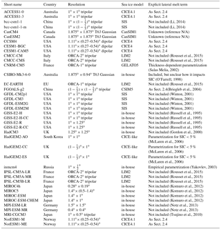
A series of experiments from different global climate models were carried out for the Coupled Model Intercomparison Project, Phase 5 (CMIP5; Taylor et al., 2012). Output is freely available online from the Program for Climate Model Diagnosis and Intercomparison. The historical experiments, which are forced by observed natural and anthropogenic forcings, end in 2005. To obtain a more contemporary overview, we also consider the first 9 years of projection experiments from the midrange mitigation emission scenario (RCP4.5). Due to the availability of observations (see below), we conduct analysis using 1992–2014. We select the first ensemble member for all models that provide monthly sea ice concentration for both the historical and RCP4.5 experiments, resulting in a set of 40 models (see Table 1).
2.2 Observations
Passive microwave radiometers deployed on satellites measure the brightness temperature of the Earth's surface, and can be used to infer sea ice concentration. There can be large differences between satellite observations (Bunzel et al., 2016), as various observational data sets apply different algorithms to convert passive-microwave signals into sea ice concentration. As summarized by Ivanova et al. (2014), differences between algorithms are caused by (1) choice of radiometer channels; (2) tie points, which are the brightness temperatures used to identify different surfaces; (3) sensitivities to changes in physical temperature of the surface; and (4) weather filters, which correct for atmospheric effects falsely indicating the presence of sea ice.
To account for some of this product uncertainty, we use three observational data sets: the Bootstrap algorithm (Comiso, 1986), the NASA Team algorithm (Cavalieri et al., 1984), and the ASI algorithm (Kaleschke et al., 2001; Spreen et al., 2008). We do not consider data sets that merge different observation methodologies. Bootstrap uses cluster analysis of brightness temperatures from two channels (19 and 37 GHz vertical polarization in the Antarctic), applies an ocean mask, and is available from 1979 at a resolution of 25 km. NASA Team uses ratios of brightness temperatures (which tends to cancel out physical temperature effects) from three channels (19 GHz in the vertical and horizontal, 37 GHz in the vertical), removes weather contamination based on certain spectral gradient ratios, and is available from 1979 at a resolution of 25 km. The ASI algorithm uses the difference in brightness temperatures between horizontal and vertical polarization at 85 GHz, uses lower-frequency channels at lower resolution to filter atmospheric effects (which are more apparent at 85 GHz than lower frequencies), and is available from 1992 at a resolution of 12 km. We choose to conduct our analysis over 1992–2014. Bootstrap and NASA Team data are available as monthly output; ASI-SSMI data are only available as daily output, so the concentration fields are averaged for each month.
(Li, 2014)(Li, 2014)(Rousset et al., 2015)(Rousset et al., 2015)(Salas Melia, 2002)(O'Farrell, 1998)(Rousset et al., 2015)(Briegleb et al., 2004)(Winton, 2001)(Winton, 2001)(Winton, 2001)(Winton, 2001)(Russell et al., 1995)(Russell et al., 1995)(Russell et al., 1995)(Russell et al., 1995)(Gordon et al., 2000)(McLaren et al., 2006)(McLaren et al., 2006)(McLaren et al., 2006)(Yakovlev, 2003)(Rousset et al., 2015)(Rousset et al., 2015)(Rousset et al., 2015)(Komuro et al., 2012)(Komuro et al., 2012)(Komuro et al., 2012)(Komuro et al., 2012)(Notz et al., 2013)(Notz et al., 2013)(Tsujino et al., 2010)Table 1CMIP5 models used in this study. SIC denotes sea ice concentration.
Differences between the three selected data sets are large: in the Antarctic, the NASA Team algorithm shows the marginal ice zone (defined as the extent of sea ice with concentration between 15 and 80 %) to extend over 2 million km more than the Bootstrap algorithm in the winter months (Stroeve et al., 2016). NASA Team is more sensitive to clouds and wind over open water than the Bootstrap mode (Andersen et al., 2006), while the high-frequency ASI algorithm is also sensitive to such atmospheric effects (Spreen et al., 2008). Bootstrap is more sensitive to physical temperature changes than NASA Team, and may underestimate concentrations at low temperatures, such as near the Antarctic coast (Comiso et al., 1997). For low concentrations, atmospheric effects, which generally lead to falsely increased sea ice, become increasingly important (Andersen et al., 2006). The weather filters/ocean masks used to correct these differ between the different algorithms.
Besides structural uncertainty in observational algorithms, systematic biases common to all three products are possible. Lack of validation data (Ivanova et al., 2014) mean it is difficult to quantify this, but accuracy is understood to be lower in the presence of melt ponds or other surface melt effects (Ivanova et al., 2014), which may act to lower retrieved concentrations; large fractions of thin ice (Ivanova et al., 2015); and stormy conditions near low concentrations (Andersen et al., 2006). Transitions between ice type can cause differences in emissivity (Grenfell and Comiso, 1986), but because models do not simulate ice types such as grease ice, this issue should not impact model–observation comparisons.
In this study, for some of the analysis we consider the three observational data sets individually. In order to compare the sea ice concentration distribution from the set of models against observations, we create an ensemble of the ASI-SSMI, Bootstrap, and NASA Team observational products. Combining the observational products in this way does have limitations, as different algorithms are likely to perform better for certain sea ice conditions and seasons. However, it is not clear from the literature where exactly the strengths of the various algorithms lie, and evaluation of the different algorithms is beyond the scope of this paper. The difficulty in ranking various observational algorithms is noted by Ivanova et al. (2014), due to a lack of validation data. They recommend constructing an ensemble of different observational products.
2.3 Metrics
Following convention, sea ice extent is defined as the area of all grid cells with more than 15 % sea ice concentration. Sea ice area is the sum of the area of all grid cells with more than 15 % sea ice concentration multiplied by the sea ice concentration in each grid cell.
To account for misplacement of sea ice, we use the integrated ice-edge error (IIEE) from Goessling et al. (2016). The IIEE describes the area of grid cells where observations and a model disagree on the presence of sea ice with concentration greater than 15 %. It can be decomposed into the total sea ice extent difference between model and observations (absolute extent error, AEE) and the difference in sea ice extent due to misplacement of sea ice (misplacement extent error, MEE). See Goessling et al. (2016) for further details.
Here, we also define an integrated ice area error (IIAE) that describes the area of sea ice on which models and observations disagree. The ice area on which models and observations disagree is likely to be more physically relevant than the area of grid cells on which models and observations disagree. The IIAE is the sum of sea ice area overestimated and underestimated,
with
and
where A is the area of interest, cm is the simulated sea ice concentration, and co is the observed sea ice concentration.
The integrated ice errors are useful as they quantify error in integrated sea ice concentration values as well as quantifying error caused by sea ice appearing in different grid cells than the observations. This is in contrast to difference in sea ice area, which accounts only for error in integrated sea ice concentration values, and difference in sea ice extent, which accounts only for error in the area of grid cells that have ice. The integrated ice errors penalize underestimation and overestimation of sea ice equally.
In this study we also consider sea ice concentration distributions, as in Notz (2014) and Ivanova et al. (2016). The sea ice concentration distribution for each model or observational product is calculated by binning grid cells according to their concentration at a 10 % spacing. The distribution is then normalized by the area of grid cells. We follow the same calculation steps as Notz (2014). This metric allows us to examine observed and modelled behaviour in different sea ice concentration regimes. It does not penalize models whose spatial distribution of sea ice disagrees with observations, but it does allow us to quantify disagreement with observations on sea ice concentration values while accounting for the observational range.
To look for behaviours which are consistent across all CMIP5 models, we compare the population of all models for the years 1992–2014 against the population of all observations for the same period. Including all models means that the range is large when models show opposite tendencies; using a multi-model mean would average out this information. Including all months in each season for all years during analysis captures sub-seasonal and inter-annual variability.
To quantify the agreement between two populations, we use the two-sample Kolmogorov–Smirnov test. This compares the empirical distribution functions of each sample, and takes into account both the location and shape of the distributions. In contrast, a Student's t test would only examine whether the means of the distributions agree. The p value obtained from the Kolmogorov–Smirnov test represents the confidence that the two populations come from the same distribution.
We found that sea ice concentration distributions show some sensitivity to grid interpolation and therefore calculate sea ice concentration distributions, as well as sea ice area, on the native model and observation grids. The integrated ice errors and differences in sea ice concentration fields between models and observations must be calculated on the same grid. In these cases, we follow Turner et al. (2013) and interpolate model output and observational data on to a common grid using the bilinear remapping function from Climate Data Operators (CDO, 2015). For the CMIP5 integrated ice errors and sea ice concentration differences, we choose a regular grid, which is a resolution equal to or higher than 20 of the 40 models and lower than all observations. We consider it to be an acceptable midpoint given the large range of model resolutions.
2.4 Coupled ocean–sea ice model
To understand the impact of model parametrizations for sea ice thermodynamics, we carry out perturbed parameter simulations using a coupled ocean–sea ice model. This consists of the ocean model NEMO and the sea ice model CICE5.1 forced with the atmospheric reanalysis JRA-55 (Japan Meteorological Agency, 2013), run on a 1∘ tripolar grid. CICE is a state-of-the-art sea ice model and is used as the sea ice component for several of the CMIP5 models (Table 1). Below we briefly explain the model's sea ice thermodynamics; further details may be found in Hunke et al. (2015).
CICE describes the evolution of the ice thickness distribution in five discrete categories. A volume of new sea ice growth is calculated from the ocean freezing/melting potential Ffrz/mlt, with new ice added as area in the smallest thickness category until the open water fraction is closed, after which it grows existing ice thickness. For sea ice melt, the net downward heat flux from the ice into the ocean, Fbot is
where ρw and cw are the density and heat capacity of sea water, ch=0.006 is the heat transfer coefficient, u* is the friction velocity, Tw is the sea surface temperature and Tf is the ocean freezing temperature, following Maykut and McPhee (1995). The balance of this flux with a conductive flux through the ice determines basal melt.
A fraction of ice is also melted laterally following Steele (1992). If floes have a mean caliper diameter L, their perimeter is p=πL and their horizontal surface area is s=αL2 (where α≈0.66 accounts for the non-circularity of floes and was determined empirically by Rothrock and Thorndike, 1984). It is assumed that melting occurs uniformly at a rate wlat around the perimeter of each floe, i.e.
Therefore the change in diameter is
For a region containing n floes with only a single diameter L, with a total horizontal area stot, the total concentration A is
Hence, with stot and n constant in time and letting the subscript o denote the initial state,
Differentiating this and inserting dL∕dt then gives the change in concentration
CICE uses a uniform lateral melt rate of
which was based on Josberger and Martin (1981), who found a complex boundary layer adjacent to vertical ice walls melting in saltwater in the laboratory, with convective motions following different flow regimes. The region adjacent to the turbulent flow regime showed the largest lateral melt rate, which could be fitted to the above relation. The coefficients m1 and m2 are the best fit to data quoted by Maykut and Perovich (1987), measured in a single static lead in the Canadian Arctic archipelago over a 3-week period. In order to apply Eq. (6), CICE assumes a single floe diameter of L=300 m throughout the ice pack. This is one of the more sophisticated schemes for lateral melt in the CMIP5 models; often it is not included at all (Table 1).
The experiments described below, which are performed with the coupled NEMO-CICE model, begin in 1979 and end in 2014. The years before 1992 are neglected to allow for model spin-up. Time series of annual maximum sea ice extent show that this takes around 10 years to stabilize. Model output from the NEMO-CICE experiments is analysed on its native grid (1∘ tripolar). Comparisons between NEMO-CICE simulations and observations (integrated ice errors and sea ice concentration differences) are computed by interpolating observations on to the same 1∘ tripolar grid using CDO (2015).
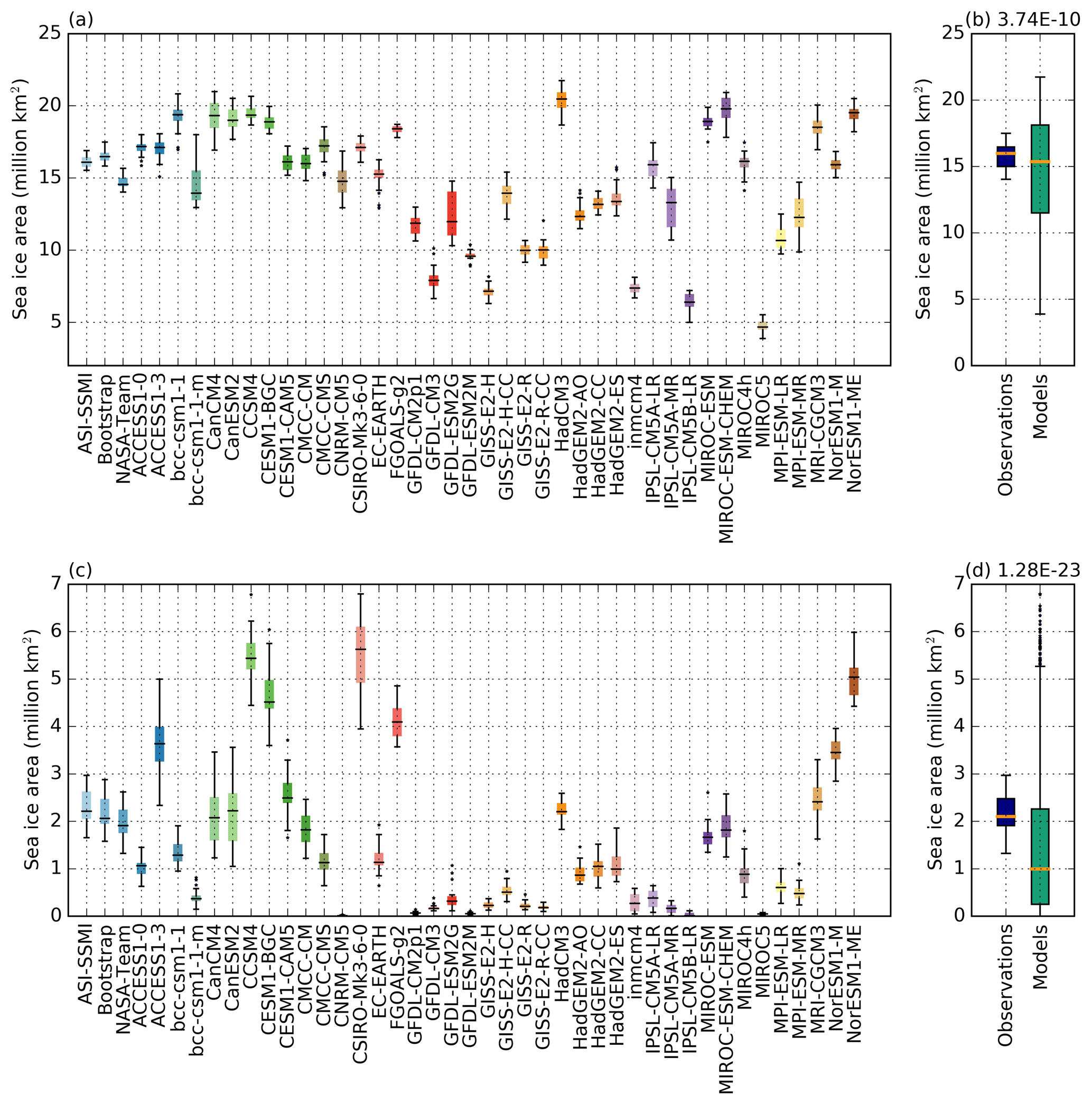
Figure 1Sea ice area for the months where the maximum (a, b) and minimum (c, d) of the seasonal cycle occur. Populations include data from all years from 1992 to 2014 with box plots for (a, c) the three observational products (ASI-SSMI, Bootstrap, and NASA Team) and all CMIP5 models listed in Table 1 individually, and (b, d) for the ensemble of observational products and the CMIP5 model ensemble. Boxes extend from the lower to upper quartile values of the data with a line at the median. Whiskers show 1.5 times the interquartile range; beyond this data are considered outliers and plotted as individual points. The text labels in (b, d) is the p value calculated from a Kolmogorov–Smirnov test, which represents the confidence that the two populations come from the same distribution.
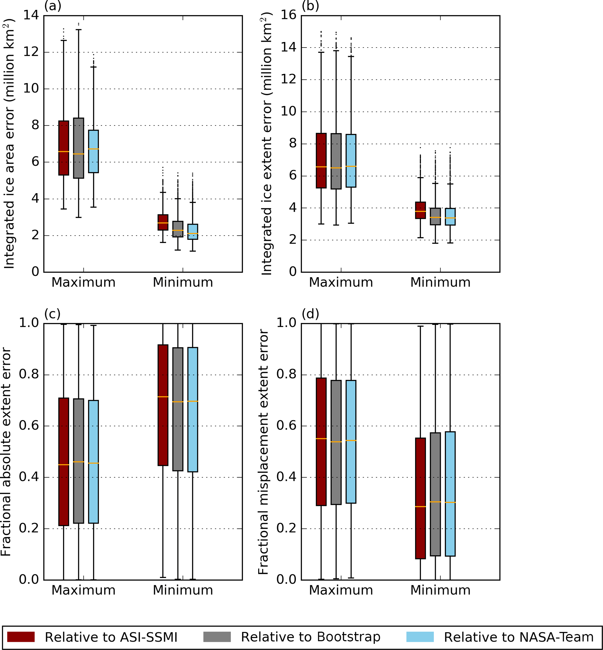
Figure 2Various ice errors for the population of CMIP5 models for all years from 1992 to 2014. Errors are shown relative to (red) the ASI-SSMI satellite observations, (grey) the Bootstrap satellite observations, and (light blue) the NASA Team observations for the months where the maximum and minimum of the seasonal cycle occur of sea ice area (a) or of sea ice extent (b, d) occur. The errors shown are the integrated ice area error (a), the integrated ice extent error (b), the absolute extent error divided by the integrated extent error (c), and the misplacement extent error divided by the integrated extent error (d). Box plots are as in Fig. 1.
Figure 1 shows sea ice area at the annual maximum and minimum from models and observations. Examining observations and models shown individually (Fig. 1a and c), we find that the interquartile range arising from inter-annual fluctuations over 1992–2014 is generally smaller than inter-model differences.
Figure 1b and d group the models and observations into two populations for comparison. At the annual maximum (Fig. 1b), the interquartile range from the ensemble of observations for 1992–2014 is contained within the ensemble of models from the same period, with the medians of the two populations in good agreement. There is no clear model tendency compared to observations for the sea ice area maximum. At the minimum (Fig. 1d), the interquartile ranges from models and observations show less overlap than the maximum, with the median from the model ensemble significantly lower than the median from the observational ensemble, suggesting a broadly consistent underestimation of sea ice area at the annual minimum by the CMIP5 models. This tendency was also noted by Turner et al. (2013) for sea ice extent. There are outliers, which show an overestimation of sea ice area, notably CSIRO-Mk-3-6-0 and the CESM models. The Kolmogorov–Smirnov test quantitatively shows that both the maximum and minimum sea ice area model–observation comparisons are significantly different, but the difference between models and observations is larger at the summer minimum than at the winter maximum (Fig. 1b and d).
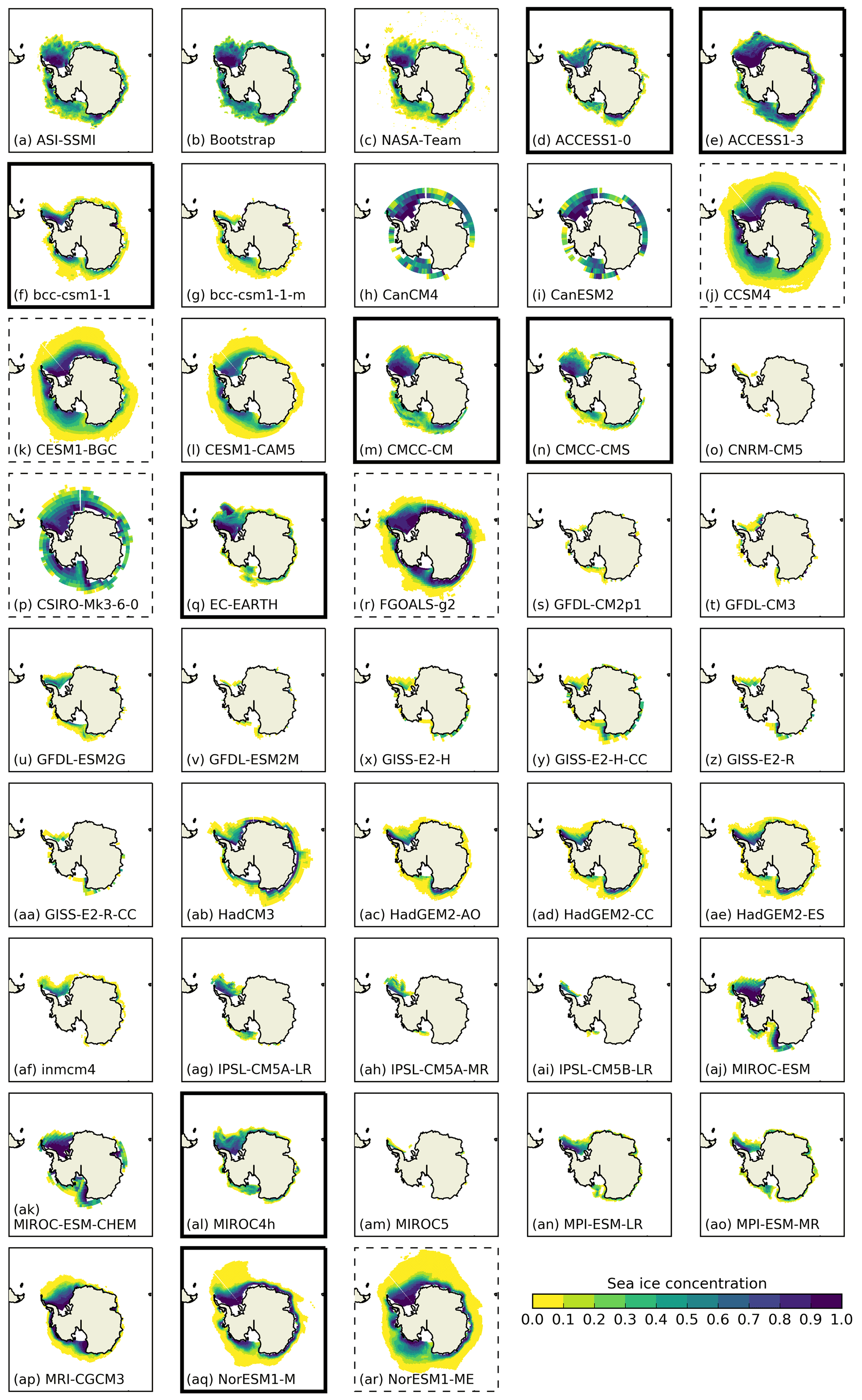
Figure 3Sea ice concentrations (above 0.1 %) for the three sets of observations (a–c) and the CMIP5 models (d–ar) for the month of each model or observation's sea ice area minimum, averaged over 1992–2014. Models marked with a bold (dashed) bounding box have high-ranked (low-ranked) integrated ice area errors regardless of observational product used. Integrated ice area errors consider sea ice concentrations >15 % for the sea ice field shown.

Figure 4The normalized sea ice concentration distribution for all months in each year from 1992 to 2014 in (a) DJF, (b) MAM, (c) JJA, and (d) SON from the three sets of satellite observations. Box plots as in Fig. 1.
The poorer performance of models at the summer minimum is supported by the integrated ice area error (Fig. 2a). The integrated ice area error has a model median value of around 2 million km2 at the sea ice area minimum and around 5.5 million km2 at the sea ice area maximum, despite a much larger amplitude in model mean sea ice area values (around 15 million and 1 million km2 respectively). Results are similar using the integrated ice extent error (Fig. 2b), although the use of extent rather than area reduces the variation between observational references. At the winter maximum, across the population of CMIP5 models and different years, we find that the absolute extent error and the misplacement extent error contribute approximately equally to the total integrated ice extent error (Fig. 2c–d). At the summer minimum, the integrated ice extent errors for the CMIP5 models have a slightly larger contribution from absolute extent errors than from misplacement area errors (Fig. 2c–d).
The large inter-model variability in extent and area at the summer minimum can be seen in Fig. 3, where the sea ice concentration fields show diverse behaviour. Variability between observational products is smaller than inter-model differences, but observational differences are visible, particularly at low concentrations. An objective way to quantify model–observation disagreement is to use the integrated ice area error, which describes the area of sea ice on which models and observations disagree. Due to observational variability, we calculate this relative to each observational product individually. The variation in observations means that we cannot rank the models in an overall order, but we can construct two groups of well-performing models and of poorly performing models whose members do not change when using different observational products. These are marked in Fig. 3.
We now consider sea ice concentration distributions from observations and models, which provide a more detailed assessment than hemisphere-integrated measures. A normalized sea ice concentration distribution may help isolate the role of the sea ice component, as models with a constant temperature bias in the atmosphere or ocean, resulting in a biased sea ice area or extent, may still simulate the relative fraction of different concentration regimes successfully.
As shown by Ivanova et al. (2016), the CMIP5 multi-model mean and the NASA Team observations have a high fraction of ice below 10 % sea ice concentration in the summer. We find that the fraction of 0.001–10 % concentration ice varies in the models from 0.005 to 1.0 (when models are essentially ice-free) in the summer (Fig. 3). It consists of up to around a third of the ice in other seasons for some models. Including these very low concentrations heavily skews the normalized sea ice concentration distribution towards low concentrations and it obscures behaviour at higher concentrations. Our aim is to look for consistent model behaviour, so to avoid the large variance between different models and between different observations at very low concentrations, we only consider sea ice concentrations above 10 %. We present all months grouped by meteorological season (December–February, DJF; March–May, MAM; June–August, JJA; and September–November, SON). This choice separates the melt season (September–February) from the freezing season (March–August), while limiting the number of months included in each season.
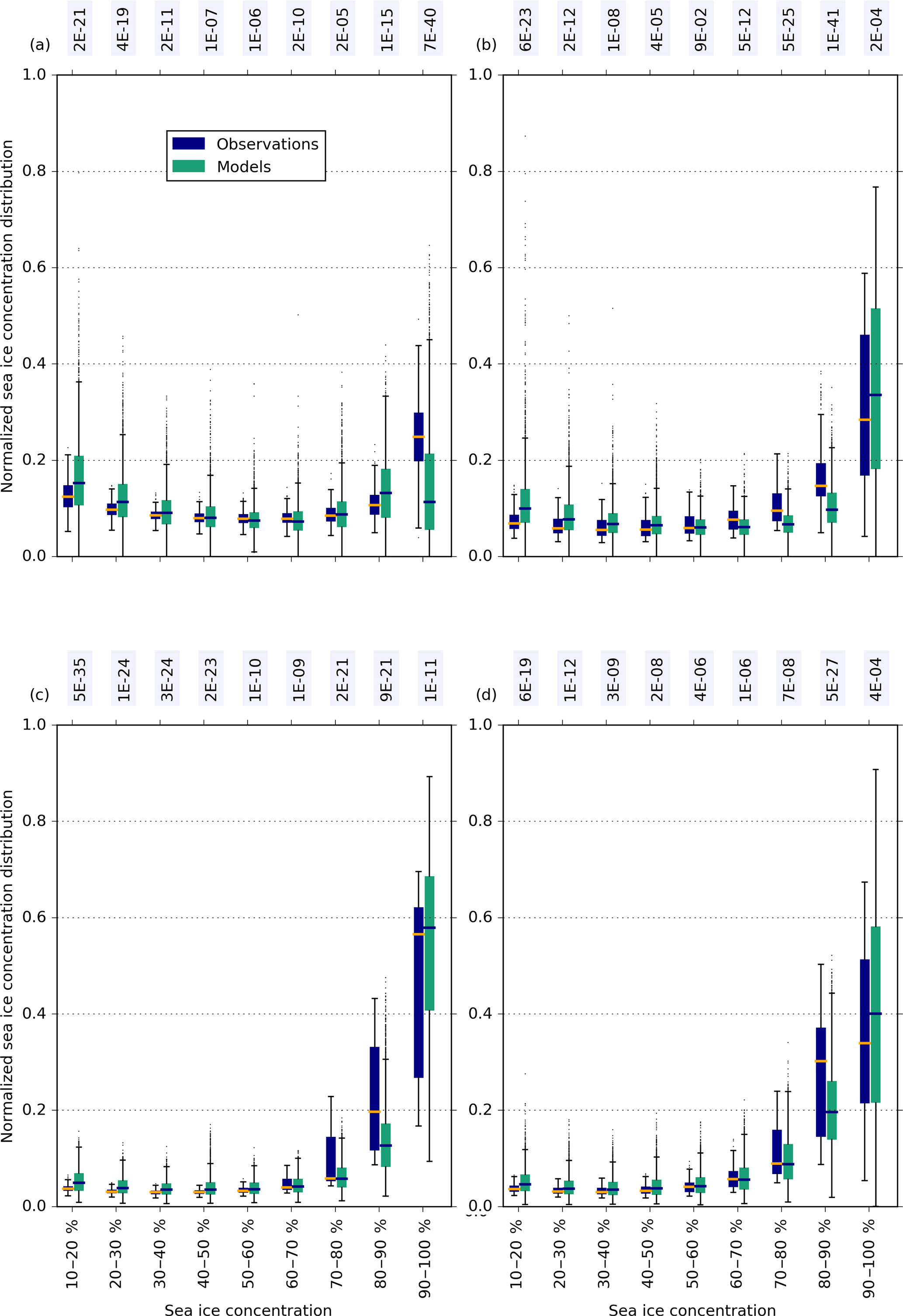
Figure 5The normalized sea ice concentration distribution for all months in each year from 1992 to 2014 in (a) DJF, (b) MAM, (c) JJA, and (d) SON from the three sets of satellite observations (blue) and the 40 CMIP5 models (green). Box plots as in Fig. 1. Annotated text is the p value calculated from a Kolmogorov–Smirnov test, which represents the confidence that the two populations come from the same distribution.
We first describe satellite observations using the normalized sea ice concentration distribution (Fig. 4). Here, individual box plots contain both inter-annual and sub-seasonal variability, while the differences between box plots reflects uncertainty arising from different processing of satellite data. Differences between observational products are largest for compact ice (90 % +) than other concentrations. In general, the ASI-SSMI observations show more similar characteristics to the Bootstrap observations than the NASA Team observations for most of the year, apart from DJF, where the opposite is true. This results in a somewhat skewed distribution when considering an ensemble created from three data sets. We find that the NASA Team algorithm shows a looser ice cover, with a significantly lower proportion of cover in the 90 % + concentration bin, than both the Bootstrap and ASI-SSMI observations. This result holds when considering an un-normalized sea ice concentration distribution as well (not shown). The fraction in the 70–90 % bins is larger to compensate. We also find that differences between data sets persists throughout the year. This is in contrast to the Arctic, where the frequency of compact sea ice cover shown in the Bootstrap and NASA Team data sets shows largest disagreement in the summer, due to issues with treatment of melt ponds (Notz, 2014). In the Antarctic, observational uncertainty in the frequency of compact sea ice is largest in winter.
Differences between the sea ice concentration distribution from models and observations, including inter-annual and sub-seasonal information (Fig. 5), are less distinct than between observational products themselves. This reflects the large range in both models and observations due to systematic uncertainties. The overall decomposition from the CMIP5 models, with a large fraction of compact ice cover and smaller fractions of lower concentrations is somewhat in agreement with observations. Agreement appears poorest in DJF, where the lower to upper quartile range for 90 % + sea ice concentration from models and observations overlap very little. Models strongly underestimate the fraction of sea ice area with concentration greater than 90 %, that is, their central ice pack is not compact enough. They tend to overestimate the fraction in the 80–90 % bin and at lower concentrations to compensate. In other seasons, there appears to be a slight tendency to overestimate the fraction of compact (90 % +) ice, with a reduction in the 70–90 % bins to compensate. The two-sample Kolmogorov–Smirnov test can be used to quantify the degree of disagreement between models and observations. The confidence level that the ensemble of observations and ensemble of models were drawn from the same population has the smallest values for the 90–100 and 10–20 % in DJF, the 70–90 % concentrations in MAM, the 10–30 % concentrations in JJA, and the 80–90 and 10–20 % concentrations in SON. There is a tendency for models to overestimate the fraction of low-concentration (10–20 %) sea ice in all seasons. This overestimation of <20 % sea ice compared to observations is robust when considering sea ice concentration bins spaced at 5 % intervals and beginning at 15 %, the cut-off used universally for sea ice extent (not shown). Unlike the other CMIP5 model tendencies, the overestimation of 10–20 % ice occurs in every month (Fig. 6), with the CMIP5 model median always outside the interquartile range of the observations.
As discussed above, this assessment takes into account observational uncertainty and inter-annual and sub-seasonal variability. That distinct tendencies arise from a population of 40 models, which contain diverse physics and different sea ice, ocean, and atmosphere models, is striking. It suggests that there is some deficiency or missing physical process common to many models.
A plausible explanation could be that models form sea ice that is too thin in the highest bin, which therefore melts more easily. Conversely, low-concentration sea ice may be too thick. However, we found no relation between these concentration biases and average sea ice thickness for the lowest and highest concentration bins (not shown). We therefore turn to lateral, rather than vertical, thermodynamics in the next section.

Figure 6The 10–20 % bin from the normalized sea ice concentration distribution for each month, where boxes contain all years from 1992 to 2014 from (blue) the three sets of satellite observations and (green) the 40 CMIP5 models. Box plots as in Fig. 1. Annotated text is the p value calculated from a Kolmogorov–Smirnov test, which represents the confidence that the two populations come from the same distribution.
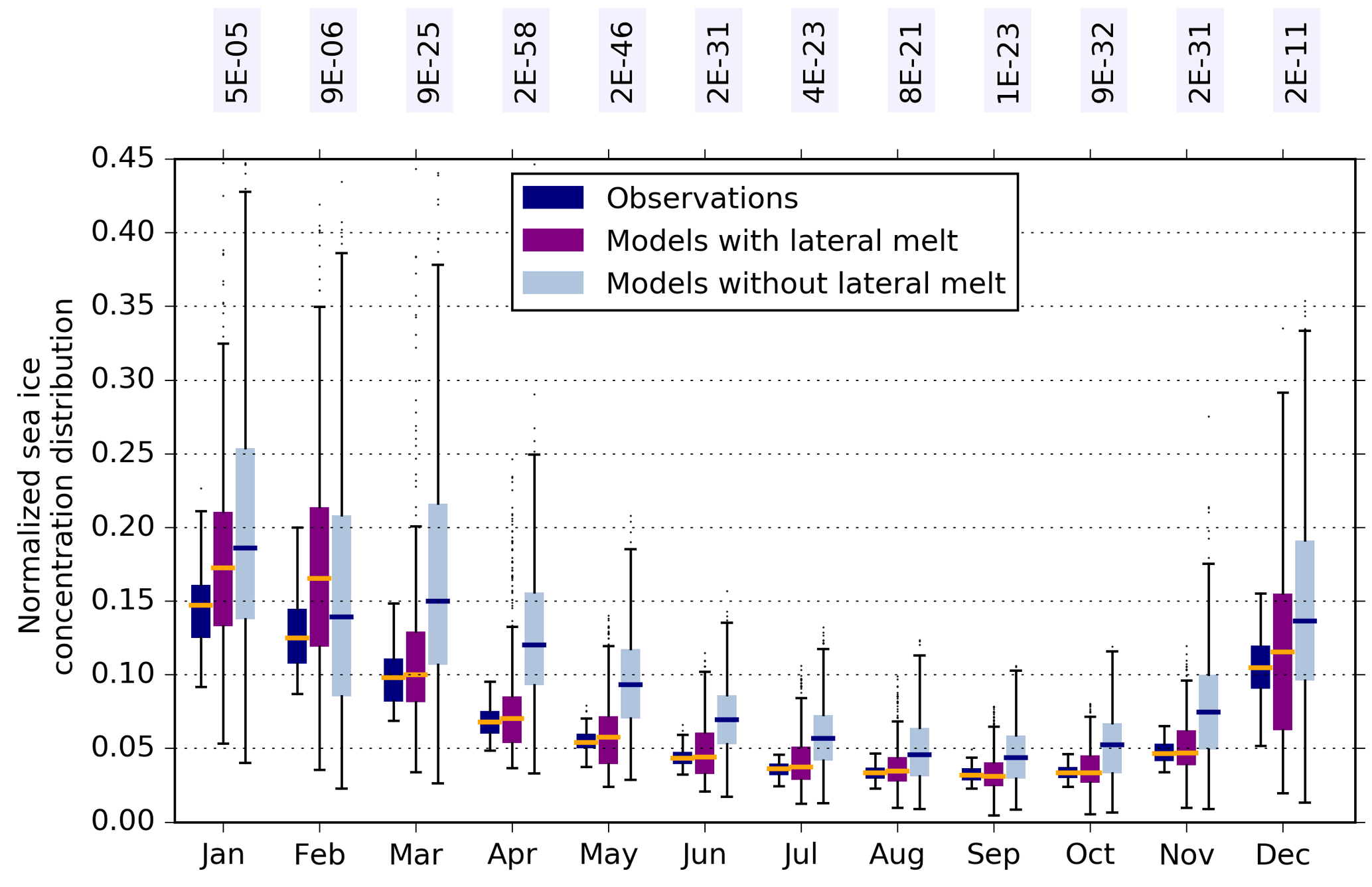
Figure 7The 10–20 % bin from the normalized sea ice concentration distribution for each month, where boxes contain all years from 1992 to 2014 from (blue) the three sets of satellite observations, (purple) CMIP5 models that include an explicit lateral melt term, and (grey) CMIP5 models that do not (from Table 1). Box plots as in Fig. 1. Annotated text is the p value calculated from a Kolmogorov–Smirnov test, which represents the confidence that the two populations come from the same distribution.
We hypothesize that the biases in low-concentration Antarctic sea ice are partially influenced by lateral floe size. Lateral floe size impacts sea ice concentration through lateral melt only if included at all in the CMIP5 models (see Table 1). Separating models with and without an explicit lateral melt term (Table 1), we find a significant difference between the two groups. Models with explicit lateral melt show a greatly reduced fraction of low-concentration ice in from March to July compared to models without, in good agreement with the observations (Fig. 7). Lateral melt can occur all year at the ice edge, where low concentrations occur.
Figure 7 demonstrates that lateral melt significantly impacts the normalized sea ice concentration distribution during autumn. However, lateral melt as it is currently included in CMIP5 models still results in a tendency towards overestimation of low-concentration sea ice in other months, and some models with an explicit lateral melt term (including the ocean–sea ice model NEMO-CICE) still simulate too large a fraction of loose ice.
We therefore proceed by examining whether changes to the lateral melt scheme may also impact the simulation of sea ice. The current representation of lateral melt in CMIP5 models is heavily parametrized (Table 1), with the formulation described in Sect. 2.4 being the most complex parametrization available in the CMIP5 models. Tsamados et al. (2015) showed that a more advanced concentration-dependent lateral melt parametrization significantly impacted the decomposition of sea ice melt processes, resulting in reduced sea ice concentrations around the ice edge in the Arctic. In the Antarctic, heat flux from solar heating of open water areas has been cited as the major cause of sea ice decay (Nihashi and Ohshima, 2001), with this melting potential available for both lateral and bottom melt. Recent studies have also suggested that floe size should also impact sea ice concentration through processes such as floe–floe collisions and lateral growth (Horvat and Tziperman, 2015; Zhang et al., 2015).
As shown in Sect. 2.4, in CICE the lateral melt flux is independent of floe size, while the change in concentration arising from lateral melt is inversely proportional to a constant floe diameter, D=300 m. In reality, sea ice floes can range in size across orders of magnitude. Several observational studies (e.g. Steer et al., 2008; Paget et al., 2001) find that the number distribution of floe sizes per unit area follows a power law with a negative exponent, suggesting that there can be a large number of small floes.
While concentration is not a proxy for floe size, in general we may expect that low-concentration areas will be made up of smaller sea ice floes than high-concentration areas because they are usually nearer the ice edge. An area of smaller sea ice floes will experience more lateral melt than an area with a larger floe size (Eq. 6). We therefore suggest that CMIP5 models using the Steele (1992) lateral melt parametrization simulate too much low-concentration sea ice because this is made up of floes smaller than 300 m and so should be subject to more lateral melt. In areas around the ice edge, which are principally low-concentration, marginal ice zone processes not included in CMIP5 models, such as wave fracture and dynamic floe interactions, may further reduce concentrations. Conversely, in high-concentration areas, floes are likely to be larger than 300 m and therefore should be subject to less lateral melt than the Steele (1992) parametrization prescribes. This could explain the underestimation of high-concentration sea ice seen in Antarctic summer.
In order to test this hypothesis, we perform three experiments using the coupled ocean–sea ice model (NEMO-CICE) described in Sect. 2.4. The experiments have identical set ups apart from a variation in L, the fixed floe diameter. We run experiments using (i) the standard value of L=300 m, (ii) a low value of L=1 m, and (iii) a high value of L=10 000 m. Our perturbed parameter values are constant and not realistic, but instead are chosen to investigate and highlight the impact of extreme changes.
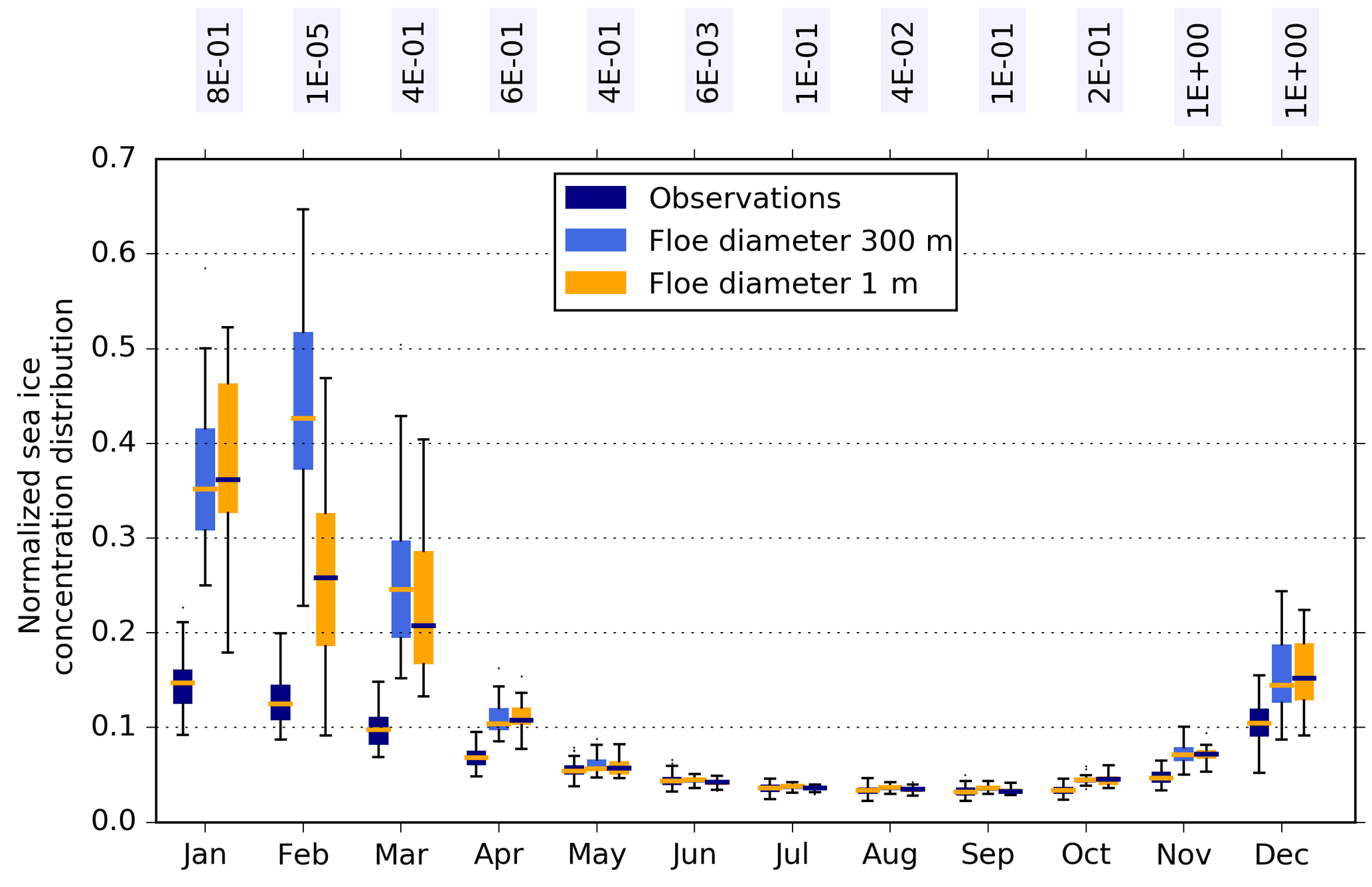
Figure 8The 10–20 % bin from the normalized sea ice concentration distribution for each month, where boxes contain all years from 1992 to 2014 from a NEMO-CICE simulation with (blue) the three sets of satellite observations, (light blue) a floe diameter of 300 m (the standard model), and (orange) a floe diameter of 1 m. Box plots as in Fig. 1. Annotated text is the p value calculated from a Kolmogorov–Smirnov test, which represents the confidence that the two populations come from the same distribution.
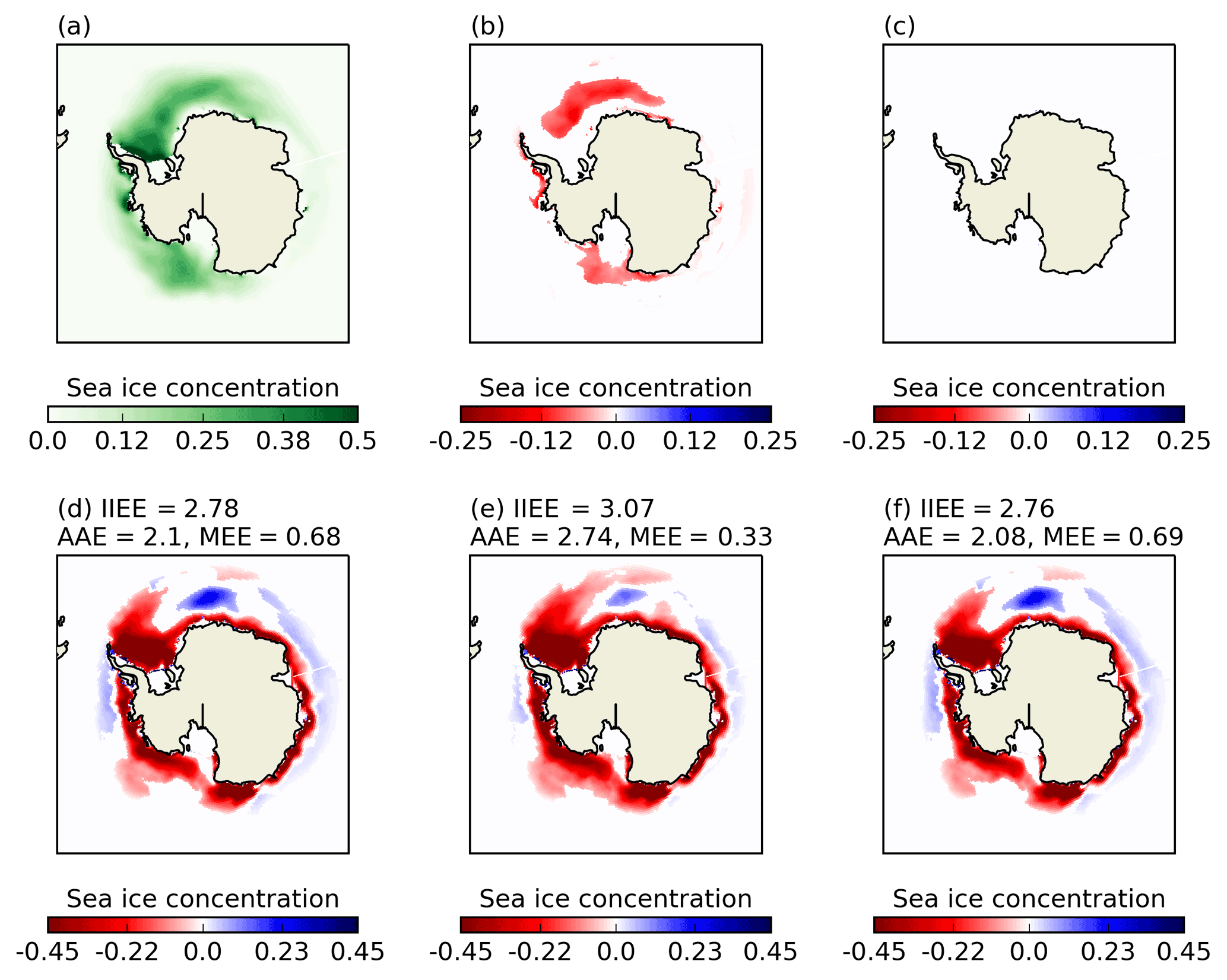
Figure 9Sea ice concentration averaged over DJF 1992–2014 for (a) the standard model simulation with a floe diameter of 300 m; (b) a model simulation with a floe diameter of 1 m (small floes) minus (a); and (c) a model simulation with a floe diameter of 10 000 m (large floes) minus (a). Panels (d–f) show simulation minus observed Bootstrap sea ice concentration, where the latter has been interpolated on to the model grid for (d) the standard model simulation, (e) the small floes simulation, and (d) the large floes simulation. In (b–f), differences are shown only if they are statistically different according to a Student's t test over 1992–2014 (p<5 %). Labels on (d–f) show the integrated ice extent error, absolute extent error and misplacement extent error in million km2.
Figure 8 shows the fraction of 10–20 % sea ice concentration from observations, the standard NEMO-CICE model and the model with reduced floe size. The standard model has very strong overestimation of low-concentration ice through December to March compared to observations. Impact of reduced floe size on the distribution is limited, with the exception of February, where there is a very strong reduction in the fraction of 10–20 % concentration ice, bringing it into better agreement with observations.
The enhanced lateral melt achieved by reducing floe size results in statistically significant reductions in sea ice concentration relative to the standard model in DJF (Fig. 9b). December, January, and February stand out from the other months in having particularly high total lateral melt rates. As expected from Fig. 6, enhanced lateral melt reduces the high bias in concentration near the outer ice edge compared to Bootstrap observations in DJF (reduction in blue, Fig. 9d and e), but enhances the low bias compared to the Bootstrap observations elsewhere (increase in red, Fig. 9d and e). We use the integrated ice extent error described above to quantify agreement with the Bootstrap observations. The same qualitative picture is obtained from all three observational products. We find that the difference in overall agreement with observations between the standard model and the small floe simulation is negligible. The absolute extent error significantly increases in the small floe simulation, because overall this simulation melts too much ice compared to observations. The misplacement extent error, however, is significantly reduced in the small floe simulation. This is partly because there is less ice to be misplaced, but also because increased lateral melt improves the distribution of sea ice around the ice edge, by melting areas where there is too much ice compared to observations (Fig. 9d and e).
Besides lateral melt, a number of other physical processes, including dynamical ones, may also contribute to an overestimation of low-concentration ice. Lecomte et al. (2016) find systematic wind-driven biases in sea ice drift speed and direction at the exterior of the Antarctic ice pack. Errors in surface winds could contribute to poor simulation of low-concentration sea ice. However, we find a very strong overestimation in low-concentration sea ice in the NEMO-CICE model, which is forced by a reanalysis atmosphere and so should not have very unrealistic winds. The dynamical response of sea ice to winds at the edge of the ice may be poorly represented, as we would expect sea ice dynamics to be floe-size dependent. Alternative rheologies (such as a granular rheology, e.g. Feltham, 2005) may be better suited to this domain. Concentrations could also be reduced by mechanical interactions between floes. However, we cannot test the impact of such floe-size-dependent processes without access to sea ice models that include them.
The impact of increased floe size, on the other hand, is much smaller (Fig. 9c and f). Differences in sea ice concentration between the standard model and the large floe simulation are barely perceptible. Changes in the ice errors relative to the standard model are of the opposite sign compared to the small floe simulation, but these changes are unlikely to be significant. Examining the basal and lateral melt rates, we find that the hemispheric average DJF 1992–2014 mean lateral melt rate accounts for only 5 % of the combined basal and lateral melt rates in the standard model. It accounts for a larger proportion (17 %) of melt in the Arctic. Decreasing floe diameter by 2 orders of magnitude increases the lateral melt rate to 83 % of the combined basal and lateral melt. This compensation effect of reduced basal melt when lateral melt is increased was also noted by Tsamados et al. (2015) in the Arctic. On the other hand, increasing the floe diameter by 2 orders of magnitude effectively switches off lateral melt (0.2 % of combined basal and lateral melt). In the latter case, more melting potential is made available for basal melting, which, because Antarctic sea ice is so thin, has the same impact on sea ice concentration as lateral melt. We conclude that there must be alternative reasons for the consistent underestimation of compact summer ice.
Looking at the regional distribution of DJF (the season where the bias is apparent in Fig. 5) seasonal mean sea ice concentration averaged over 1992–2014, high-concentration (90–100 %) ice appears in the observations mean only in the Weddell Sea (Fig. 3). Taking the difference between the high-concentration ice in each observational product and the sea ice concentration in the CMIP5 model simulations shows that very few of the models simulate high enough concentrations in this area. Figure 10 shows the difference between the ASI-SSMI observations and the CMIP5 models; differences are slightly enhanced using Bootstrap and less pronounced when using NASA Team. This demonstrates a consistent model tendency to underestimate concentrations in the Weddell Sea, the largest region of multi-year ice in Antarctica. The bias is not present in other seasons, suggesting it is related to overestimated melt or break-up processes, including misrepresentation of sea ice dynamics.
Overestimated melt or break-up could be a result of the sea ice model or a biased warm atmosphere or ocean. While consideration of normalized sea ice concentration distribution is intended to remove overall biases caused by (for example) a warm ocean, in summer the warm ocean could shift the whole distribution to lower concentrations. Alternatively, or likely in conjunction with this, regionally important processes may be being misrepresented. Evaluating the ORCA2-LIM coupled ocean–sea ice model, Timmermann et al. (2004) found that overestimation of westerly winds led to an underestimation of sea ice coverage on the eastern side of the Antarctic peninsula, in the Weddell Sea. Other CMIP5 models may simulate high drift speeds due to winds or sea ice rheology, which Lecomte et al. (2016) found correlated with a faster sea ice retreat.
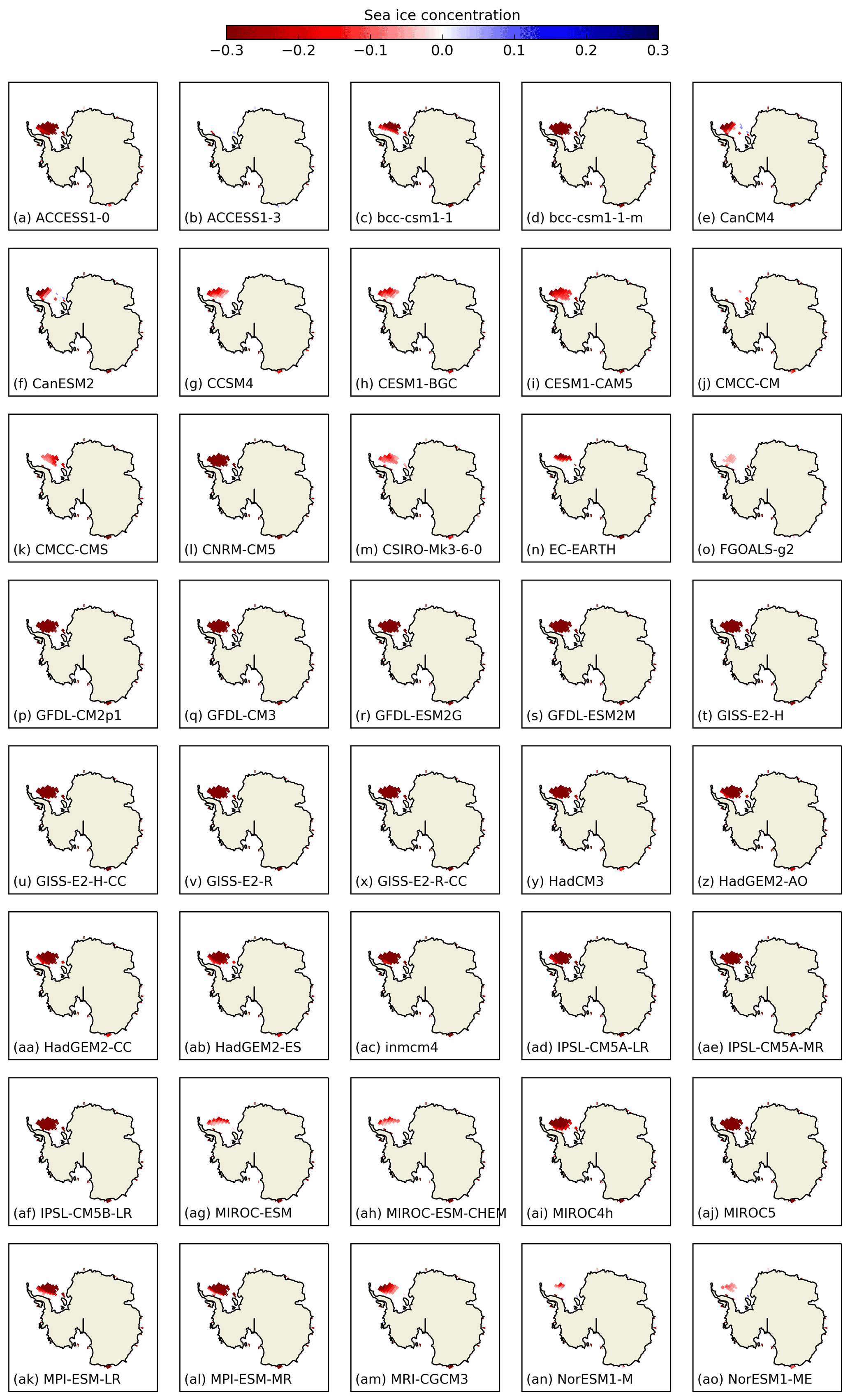
Figure 10Simulation minus observed ASI-SSMI sea ice concentration for DJF 1992–2014 for each CMIP5 model, where only grid cells with observational mean sea ice concentration is ≥90 % are considered. Differences are only shown if they are statistically different according to a Student's t test over 1992–2014 (p<5 %).
In this study, we examine the distribution of sea ice concentration from both models and observations. Firstly, we show that observed sea ice concentration values can differ significantly between three widely used algorithms for satellite data. This observational uncertainty provides a limit beyond which we cannot further evaluate model agreement with observations. Many sea ice model–observation comparisons use only one satellite data set assumed to represent the true observed state, an approach which may be sufficient when using sea ice extent, a metric where the various algorithms broadly agree. However, when using metrics that go beyond sea ice extent, using for example sea ice area or sea ice concentration distributions, model evaluation studies should account for the observational range.
We find that simulation of high-concentration (90 % +) sea ice in models is in better agreement with the NASA Team observations than the observational range including the Bootstrap and ASI-SSMI observations, in agreement with Ivanova et al. (2016), who only examined the CMIP5 multi-model mean.
Accounting for the range in three observational products, we find that models overestimate the extent of low-concentration sea ice throughout the year, while underestimating the extent of high-concentration sea ice in summer. This common behaviour across diverse models with varying physics is a result not previously highlighted and warrants further attention.
We note that using the observational range as an uncertainty estimate neglects biases that are common to the three different satellite observations. As mentioned above, sea ice concentrations are considered to be most uncertain during melt conditions, for large fractions of thin ice and at low concentrations during storms. In the context of the results from the model–observation comparison for normalized sea ice concentration distributions, we suggest that the impact of uncertainty of melt conditions is limited as the high bias in low-concentration ice from CMIP5 models is visible throughout the year. The low bias in high-concentration ice during the melt season would be strengthened if observations were underestimating ice concentrations in this season. Inclusion of both NASA Team and Bootstrap algorithms, with the former tending to cancel out physical temperature effects, will sample some of this uncertainty.
The underestimation of sea ice concentrations in areas of thin ice (<35 cm) (Ivanova et al., 2015) may cause a bias at any concentration in the observed normalized sea ice concentration distribution from observations, with the possibility of a positive bias in the very lowest concentrations. Stormy conditions near the ice edge lead to false sea ice concentrations near the ice edge; weather filters may accurately remove these, leave them uncorrected (Andersen et al., 2006), or erroneously remove real sea ice. The latter may underestimate low concentrations. Spreen et al. (2008) suggest the filter method used in ASI-SSMI observations may result in a positive bias in the marginal ice zone, and Steffen and Schweiger (1991) found that the NASA Team algorithm overestimates low-concentration ice when compared to Landsat imagery. Considering all this evidence we suggest that the magnitude or sign of any systematic biases in satellite radiometer observations is unclear when comparing with climate models. This is particularly true for low concentrations. Here the use of different approaches to weather filters within the different algorithms may assist in sampling observational uncertainty. Development of sea ice satellite emulators, which use climate model output to calculate brightness temperatures (e.g. Tonboe et al., 2011), may help to reduce uncertainty when comparing models to observations in the future.
Categorizing models according to whether they explicitly represent lateral melting, which is the only thermodynamic sea ice process that reduces concentrations in models regardless of sea ice thickness, we find a strong impact of this process on low-concentration sea ice. In Sect. 2.4 we briefly review typical sea ice model thermodynamics, and in particular the change in concentration induced by lateral melt rate for a region containing floes of a single diameter, which follows Steele (1992). Horvat et al. (2016) finds that development of ocean eddies due to lateral density gradients could induce much larger lateral melt than that suggested from the Steele (1992) geometric model. This would support increasing the lateral melt rate in models, as we have done artificially here through a reduced constant floe size. Heat budget analysis (Nihashi and Ohshima, 2001) and modelling studies (Fichefet and Maqueda, 1997; Ohshima and Nihashi, 2005) suggest that the major cause of Antarctic sea ice decay is atmospheric heat input to open water, which causes bottom and lateral melt. Fichefet and Maqueda (1997) find that sea ice melt by open water plays a larger role in the Antarctic than in the Arctic. We further note that the coefficients in the lateral melt rate used in CICE were measured in the Arctic only (Maykut and Perovich, 1987) and few, if any, observational studies exist on the relative importance of bottom and lateral melt in the Antarctic.
The impacts of enhancing lateral melt via reducing a constant floe size shown here suggest that this process should not be applied in the same way throughout the ice pack. While not all models include such a lateral melt parametrization, the biases at the tails of the concentration distributions from the CMIP5 models point to inclusion of model processes that are not suitable for both high-concentration and low-concentration regimes. A possible conclusion, therefore, is that physics in sea ice models are not heterogeneous enough to represent observed sea ice cover. Given the possible contribution of dynamic processes to model biases in the sea ice concentration distribution, a full exploration of sea ice dynamics for all CMIP5 models using the sea ice concentration budget decomposition of Uotila et al. (2014) would be welcome. Including information on the floe size distribution and floe size dependent processes (e.g. Horvat and Tziperman, 2015; Zhang et al., 2016; Bennetts et al., 2017) could improve consistency with observations in the metrics presented here.
CMIP5 data are available at http://cmip-pcmdi.llnl.gov/cmip5/data_portal.html. ASI-SSMI data are available at http://icdc.cen.uni-hamburg.de/1/daten/cryosphere/seaiceconcentration-asi-ssmi.html (Kaleschke et al., 2016). Bootstrap and NASA Team data are available at https://nsidc.org/data/g02202/versions/3 (Meier et al., 2017). NEMO-CICE model output is available from the corresponding author upon request.
LR and SD designed the analysis and experiments and LR carried them out. LR prepared the manuscript with contributions from all co-authors.
The authors declare that they have no conflict of interest.
The authors wish to thank Erik Behrens and Jonny Williams for assistance
setting up and running the coupled ocean–sea ice model, Stephen Stuart for
assistance with CMIP5 output acquisition, and Cecilia Bitz for helpful
discussions in the early stages of this work. We are grateful to the
reviewers, whose comments significantly improved the manuscript. This
research was funded via Marsden contract VUW-1408. We acknowledge the World
Climate Research Programme's Working Group on Coupled Modelling, which is
responsible for CMIP, and we thank the climate modelling groups (listed in
Table 1 of this paper) for producing and making available their model output.
For CMIP the U.S. Department of Energy's Program for Climate Model Diagnosis
and Intercomparison provides coordinating support and led development of
software infrastructure in partnership with the Global Organization for Earth
System Science Portals.
Edited by: Dirk Notz
Reviewed by: Francois Massonnet and one anonymous referee
Andersen, S., Tonboe, R., Kern, S., and Schyberg, H.: Improved retrieval of sea ice total concentration from spaceborne passive microwave observations using numerical weather prediction model fields: an intercomparison of nine algorithms, Remote Sens. Environ., 104, 374–392, https://doi.org/10.1016/j.rse.2006.05.013, 2006. a, b, c, d
Asplin, M. G., Scharien, R., Else, B., Howell, S., Barber, D. G., Papakyriakou, T., and Prinsenberg, S.: Implications of fractured Arctic perennial ice cover on thermodynamic and dynamic sea ice processes, J. Geophys. Res.-Oceans, 119, 2327–2343, 2014. a
Bennetts, L. G., O'Farrell, S., and Uotila, P.: Brief communication: Impacts of ocean-wave-induced breakup of Antarctic sea ice via thermodynamics in a stand-alone version of the CICE sea-ice model, The Cryosphere, 11, 1035–1040, https://doi.org/10.5194/tc-11-1035-2017, 2017. a
Bentsen, M., Bethke, I., Debernard, J. B., Iversen, T., Kirkevåg, A., Seland, Ø., Drange, H., Roelandt, C., Seierstad, I. A., Hoose, C., and Kristjánsson, J. E.: The Norwegian Earth System Model, NorESM1-M – Part 1: Description and basic evaluation of the physical climate, Geosci. Model Dev., 6, 687–720, https://doi.org/10.5194/gmd-6-687-2013, 2013. a
Briegleb, B., Bitz, C. M., Hunke, E. C., Lipscomb, W. H., Holland, M. M., Schramm, J., and Moritz, R.: Scientific Description of the Sea Ice Component in the Community Climate System Model, Version Three. NCAR/TN-463+STR, NCAR Tech. Note, NCAR, Boulder, Colorado, USA, 1–78, 2004. a
Bunzel, F., Notz, D., Baehr, J., Muller, W. A., and Frohlich, K.: Seasonal climate forecasts significantly affected by observational uncertainty of Arctic sea ice concentration, Geophys. Res. Lett., 43, 852–859, https://doi.org/10.1002/2015GL066928, 2016. a
Cavalieri, D. J., Gloersen, P., and Campbell, W. J.: Determination of sea ice parameters with the NIMBUS 7 SMMR, J. Geophys. Res.-Atmos., 89, 5355–5369, https://doi.org/10.1029/JD089iD04p05355, 1984. a
CDO: Climate Data Operators, available at: http://www.mpimet.mpg.de/cdo (last access: November 2017), 2015. a, b
Comiso, J. C.: Characteristics of Arctic winter sea ice from satellite multispectral microwave observations, J. Geophys. Res.-Oceans, 91, 975–994, https://doi.org/10.1029/JC091iC01p00975, 1986. a
Comiso, J. C., Cavalieri, D. J., Parkinson, C. L., and Gloersen, P.: Passive microwave algorithms for sea ice coneentration: a comparison of two techniques, Remote Sens. Environ., 60, 357–384, https://doi.org/10.1016/S0034-4257(96)00220-9, 1997. a
Feltham, D. L.: Granular flow in the marginal ice zone, Philos. T. Roy. Soc. A, 363, 1677–1700, 2005. a
Fichefet, T. and Maqueda, M. A. M.: Sensitivity of a global sea ice model to the treatment of ice thermodynamics and dynamics, J. Geophys. Res.-Oceans, 102, 12609–12646, https://doi.org/10.1029/97JC00480, 1997. a, b
Goessling, H. F., Tietsche, S., Day, J. J., Hawkins, E., and Jung, T.: Predictability of the Arctic sea ice edge, Geophys. Res. Lett., 43, 1642–1650, https://doi.org/10.1002/2015GL067232, 2016. a, b
Goosse, H., Campin, J. M., Fichefet, T., and Deleersnijder, E.: Impact of sea-ice formation on the properties of Antarctic Bottom Water, Ann. Glaciol., 25, 276–281, 1997. a
Gordon, C., Cooper, C., Senior, C. A., Banks, H., Gregory, J. M., Johns, T. C., Mitchell, J. F. B., and Wood, R. A.: The simulation of SST, sea ice extents and ocean heat transports in a version of the Hadley Centre coupled model without flux adjustments, Clim. Dynam., 16, 147–168, 2000. a, b
Grenfell, T. C. and Comiso, J. C.: Multifrequency Passive Microwave Observations of First-Year Sea Ice Grown in a Tank, IEEE T. Geosci. Remote, GE-24, 826–831, https://doi.org/10.1109/TGRS.1986.289696, 1986. a
Horvat, C. and Tziperman, E.: A prognostic model of the sea-ice floe size and thickness distribution, The Cryosphere, 9, 2119–2134, https://doi.org/10.5194/tc-9-2119-2015, 2015. a, b
Horvat, C., Tziperman, E., and Campin, J. M.: Interaction of sea ice floe size, ocean eddies and sea ice melting, Geophys. Res. Lett., 43, 8083–8090, https://doi.org/10.1002/2016GL069742, 2016. a
Hunke, E. C., Lipscomb, W. H., Turner, A. K., Jeffery, N., and Elliott, S.: CICE: the Los Alamos Sea Ice Model Documentation and Software User's Manual Version 5.1, Tech. rep., Los Alamos Natl. Laboratory, Los Alamos, NM, USA, 2015. a, b
Ivanova, D. P., Gleckler, P. J., Taylor, K. E., Durack, P. J., and Marvel, K. D.: Moving beyond the total sea ice extent in gauging model biases, J. Climate, 29, 8965–8987, https://doi.org/10.1175/jcli-d-16-0026.1, 2016. a, b, c, d, e
Ivanova, N., Johannessen, O. M., Pedersen, L. T., and Tonboe, R. T.: Retrieval of Arctic sea ice parameters by satellite passive microwave sensors: A comparison of eleven sea ice concentration algorithms, IEEE T. Geosci. Remote, 52, 7233–7246, 2014. a, b, c, d
Ivanova, N., Pedersen, L. T., Tonboe, R. T., Kern, S., Heygster, G., Lavergne, T., Sørensen, A., Saldo, R., Dybkjær, G., Brucker, L., and Shokr, M.: Inter-comparison and evaluation of sea ice algorithms: towards further identification of challenges and optimal approach using passive microwave observations, The Cryosphere, 9, 1797–1817, https://doi.org/10.5194/tc-9-1797-2015, 2015. a, b
Japan Meteorological Agency: JRA-55: Japanese 55-year Reanalysis, Daily 3-Hourly and 6-Hourly Data, https://doi.org/10.5065/D6HH6H41, 2013. a
Josberger, E. G. and Martin, S.: A laboratory and theoretical study of the boundary layer adjacent to a vertical melting ice wall in salt water, J. Fluid Mech., 111, 439–473, 1981. a
Kaleschke, L., Lupkes, C., Vihma, T., Haarpaintner, J., Bochert, A., Hartmann, J., and Heygster, G.: SSM/I sea ice remote sensing for mesoscale ocean-atmosphere interaction analysis, Can. J. Remote Sens., 27, 526–537, 2001. a
Kaleschke, L., Girard-Ardhuin, F., Spreen, G., Beitsch, A., and Kern, S.: ASI Algorithm SSMI-SSMIS sea ice concentration data, originally computed at and provided by IFREMER, Brest, France, obtained as 5-day median-filtered and gap-filled product for 1992–2014 from the Integrated Climate Date Center (ICDC), University of Hamburg, Hamburg, Germany, available at: http://icdc.cen.uni-hamburg.de/1/daten/cryosphere/seaiceconcentration-asi-ssmi.html, last access: 8 July 2016. a
Komuro, Y., Suzuki, T., Sakamoto, T. T., Hasumi, H., Ishii, M., Watanabe, M., Nozawa, T., Yokohata, T., Nishimura, T., Ogochi, K., Emori, S., and Kimoto, M.: Sea-Ice in Twentieth-Century simulations by new MIROC coupled models: A comparison between models with high resolution and with ice thickness distribution, J. Meteorol. Soc. Jpn., 90A, 213–232, https://doi.org/10.2151/jmsj.2012-A11, 2012. a, b, c, d
Lecomte, O., Goosse, H., Fichefet, T., Holland, P. R., Uotila, P., Zunz, V., and Kimura, N.: Impact of surface wind biases on the Antarctic sea ice concentration budget in climate models, Ocean Model., 105, 60–70, https://doi.org/10.1016/j.ocemod.2016.08.001, 2016. a, b
Li, L.: An overview of BCC climate system model development and application for climate change studies, J. Meteorol. Res.-Prc., 28, 34–56, 2014. a, b
Mahlstein, I., Gent, P. R., and Solomon, S.: Historical Antarctic mean sea ice area, sea ice trends, and winds in CMIP5 simulations, J. Geophys. Res.-Atmos., 118, 5105–5110, https://doi.org/10.1002/jgrd.50443, 2013. a
Maykut, G. A. and McPhee, M. G.: Solar heating of the Arctic mixed layer, J. Geophys. Res.-Oceans, 100, 24691–24703, https://doi.org/10.1029/95JC02554, 1995. a
Maykut, G. A. and Perovich, D. K.: The role of shortwave radiation in the summer decay of a sea ice cover, J. Geophys. Res.-Oceans, 92, 7032–7044, https://doi.org/10.1029/JC092iC07p07032, 1987. a, b
McLaren, A. J., Banks, H. T., Durman, C. F., Gregory, J. M., Johns, T. C., Keen, A. B., Ridley, J. K., Roberts, M. J., Lipscomb, W. H., Connolley, W. M., and Laxon, S. W.: Evaluation of the sea ice simulation in a new coupled atmosphere-ocean climate model (HadGEM1), J. Geophys. Res.-Oceans, 111, C12014, https://doi.org/10.1029/2005JC003033, 2006. a, b, c
Meier, W., Fetterer, F., Savoie, M., Mallory, S., Duerr, R., and Stroeve, J.: NOAA/NSIDC Climate Data Record of Passive Microwave Sea Ice Concentration, Version 3. NASA Team and Bootstrap products, NSIDC (National Snow and Ice Data Center), Boulder, Colorado, USA, last accessed: 22 August 2017, https://doi.org/10.7265/N59P2ZTG, 2017. a
Nihashi, S. and Ohshima, K. I.: Relationship between ice decay and solar heating through open water in the Antarctic sea ice zone, J. Geophys. Res.-Oceans, 106, 16767–16782, https://doi.org/10.1029/2000JC000399, 2001. a, b
Notz, D.: Sea-ice extent and its trend provide limited metrics of model performance, The Cryosphere, 8, 229–243, https://doi.org/10.5194/tc-8-229-2014, 2014. a, b, c, d, e
Notz, D.: How well must climate models agree with observations?, Philos. T. Roy. Soc. A, 373, https://doi.org/10.1098/rsta.2014.0164, 2015. a
Notz, D., Haumann, F. A., Haak, H., Jungclaus, J. H., and Marotzke, J.: Arctic sea-ice evolution as modeled by Max Planck Institute for Meteorology's Earth system model, J. Adv. Model. Earth Sy., 5, 173–194, https://doi.org/10.1002/jame.20016, 2013. a, b
O'Farrell, S. P.: Investigation of the dynamic sea ice component of a coupled atmosphere-sea ice general circulation model, J. Geophys. Res.-Oceans, 103, 15751–15782, https://doi.org/10.1029/98JC00815, 1998. a
Ohshima, K. I. and Nihashi, S.: A simplified ice–ocean coupled model for the Antarctic ice melt season, J. Phys. Oceanogr., 35, 188–201, https://doi.org/10.1175/jpo-2675.1, 2005. a
Paget, M., Worby, A., and Michael, K.: Determining the floe-size distribution of East Antarctic sea ice from digital aerial photographs, Ann. Glaciol., 33, 94–100, 2001. a
Previdi, M., Smith, K. L., and Polvani, L. M.: How well do the CMIP5 models simulate the Antarctic atmospheric energy budget?, J. Climate, 28, 7933–7942, https://doi.org/10.1175/jcli-d-15-0027.1, 2015. a
Rosenblum, E. and Eisenman, I.: Faster arctic sea ice retreat in CMIP5 than in CMIP3 due to volcanoes, J. Climate, 29, 9179–9188, https://doi.org/10.1175/JCLI-D-16-0391.1, 2016. a
Rothrock, D. and Thorndike, A.: Measuring the sea ice floe size distribution, J. Geophys. Res.-Oceans, 89, 6477–6486, 1984. a
Rousset, C., Vancoppenolle, M., Madec, G., Fichefet, T., Flavoni, S., Barthélemy, A., Benshila, R., Chanut, J., Levy, C., Masson, S., and Vivier, F.: The Louvain-La-Neuve sea ice model LIM3.6: global and regional capabilities, Geosci. Model Dev., 8, 2991–3005, https://doi.org/10.5194/gmd-8-2991-2015, 2015. a, b, c, d, e, f
Russell, G., Miller, J., and Rind, D.: A coupled atmosphere-ocean model for transient climate change studies, Atmos. Ocean, 33, 683–730, 1995. a, b, c, d
Salas Melia, D.: A global coupled sea ice-ocean model, Ocean Model., 4, 137–172, https://doi.org/10.1016/S1463-5003(01)00015-4, 2002. a
Shu, Q., Song, Z., and Qiao, F.: Assessment of sea ice simulations in the CMIP5 models, The Cryosphere, 9, 399–409, https://doi.org/10.5194/tc-9-399-2015, 2015. a
Spreen, G., Kaleschke, L., and Heygster, G.: Sea ice remote sensing using AMSR-E 89-GHz channels, J. Geophys. Res.-Oceans, 113, C02S03, https://doi.org/10.1029/2005JC003384, 2008. a, b, c
Steele, M.: Sea ice melting and floe geometry in a simple ice-ocean model, J. Geophys. Res.-Oceans, 97, 17729–17738, 1992. a, b, c, d, e
Steer, A., Worby, A., and Heil, P.: Observed changes in sea-ice floe size distribution during early summer in the western Weddell Sea, Deep-Sea Res. Pt. II, 55, 933–942, https://doi.org/10.1016/j.dsr2.2007.12.016, 2008. a
Steffen, K. and Schweiger, A.: NASA team algorithm for sea ice concentration retrieval from Defense Meteorological Satellite Program special sensor microwave imager: comparison with Landsat satellite imagery, J. Geophys. Res.-Oceans, 96, 21971–21987, https://doi.org/10.1029/91JC02334, 1991. a
Stroeve, J. C., Kattsov, V., Barrett, A., Serreze, M., Pavlova, T., Holland, M., and Meier, W. N.: Trends in Arctic sea ice extent from CMIP5, CMIP3 and observations, Geophys. Res. Lett., 39, L16502 , https://doi.org/10.1029/2012GL052676, 2012. a
Stroeve, J. C., Jenouvrier, S., Campbell, G. G., Barbraud, C., and Delord, K.: Mapping and assessing variability in the Antarctic marginal ice zone, pack ice and coastal polynyas in two sea ice algorithms with implications on breeding success of snow petrels, The Cryosphere, 10, 1823–1843, https://doi.org/10.5194/tc-10-1823-2016, 2016. a
Taylor, K. E., Stouffer, R. J., and Meehl, G. A.: An overview of CMIP5 and the experiment design, B. Am. Meteorol. Soc., 93, 485–498, https://doi.org/10.1175/BAMS-D-11-00094.1, 2012. a
Timmermann, R., Worby, A., Goosse, H., and Fichefet, T.: Utilizing the ASPeCt sea ice thickness data set to evaluate a global coupled sea ice–ocean model, J. Geophys. Res.-Oceans, 109, C07017, https://doi.org/10.1029/2003JC002242, 2004. a
Tonboe, R. T., Dybkjaer, G., and Høyer, J. L.: Simulations of the snow covered sea ice surface temperature and microwave effective temperature, Tellus A, 63, 1028–1037, https://doi.org/10.1111/j.1600-0870.2011.00530.x, 2011. a
Tsamados, M., Feltham, D., Petty, A., Schroeder, D., and Flocco, D.: Processes controlling surface, bottom and lateral melt of Arctic sea ice in a state of the art sea ice model, Philos. T. Roy. Soc., A, 373, 30, https://doi.org/10.1098/rsta.2014.0167, 2015. a, b
Tsujino, H., Motoi, T., Ishikawa, I., Hirabara, M., Nakano, H., Yamanaka, G., Yasuda, T., and Ishizaki, H.: Reference manual for the Meteorological Research Institute community ocean model (MRI. COM) version 3, Technical Reports of the Meteorological Research Institute, Tsukuba, Japan, 59, 241, 2010. a
Turner, J., Bracegirdle, T. J., Phillips, T., Marshall, G. J., and Hosking, J. S.: An initial assessment of Antarctic sea ice extent in the CMIP5 models, J. Climate, 26, 1473–1484, 2013. a, b, c
Uotila, P., Holland, P. R., Vihma, T., Marsland, S. J., and Kimura, N.: Is realistic Antarctic sea-ice extent in climate models the result of excessive ice drift?, Ocean Model., 79, 33–42, https://doi.org/10.1016/j.ocemod.2014.04.004, 2014. a
Winton, M.: FMS Sea Ice Simulator, GFDL Tech. Document, Geophysical Fluid Dynamics Laboratory, Princeton, 2001. a, b, c, d
Yakovlev, N.: Coupled model of ocean general circulation and sea ice evolution in the Arctic Ocean, Izv. Atmos. Ocean. Phy.+, 39, 355–368, 2003. a
Zhang, J., Schweiger, A., Steele, M., and Stern, H.: Sea ice floe size distribution in the marginal ice zone: Theory and numerical experiments, J. Geophys. Res.-Oceans, 120, 3484–3498, 2015. a
Zhang, J., Stern, H., Hwang, B., Schweiger, A., Steele, M., Stark, M., and Graber, H. C.: Modeling the seasonal evolution of the Arctic sea ice floe size distribution, Elementa: Science of the Anthropocene, 4, 000126, https://doi.org/10.12952/journal.elementa.000126, 2016. a
Zunz, V., Goosse, H., and Massonnet, F.: How does internal variability influence the ability of CMIP5 models to reproduce the recent trend in Southern Ocean sea ice extent?, The Cryosphere, 7, 451–468, https://doi.org/10.5194/tc-7-451-2013, 2013. a