the Creative Commons Attribution 4.0 License.
the Creative Commons Attribution 4.0 License.
 | 29 Nov 2018
Comparison of four calving laws to model Greenland outlet glaciers
Mathieu Morlighem
Michael Wood
Johannes H. Bondzio
Calving is an important mechanism that controls the dynamics of marine terminating glaciers of Greenland. Iceberg calving at the terminus affects the entire stress regime of outlet glaciers, which may lead to further retreat and ice flow acceleration. It is therefore critical to accurately parameterize calving in ice sheet models in order to improve the projections of ice sheet change over the coming decades and reduce the uncertainty in their contribution to sea-level rise. Several calving laws have been proposed, but most of them have been applied only to a specific region and have not been tested on other glaciers, while some others have only been implemented in 1-D flowline or vertical flowband models. Here, we test and compare several calving laws recently proposed in the literature using the Ice Sheet System Model (ISSM). We test these calving laws on nine tidewater glaciers of Greenland. We compare the modeled ice front evolution to the observed retreat from Landsat data collected over the past 10 years, and assess which calving law has better predictive abilities for each glacier. Overall, the von Mises tensile stress calving law is more satisfactory than other laws for simulating observed ice front retreat, but new parameterizations that better capture the different modes of calving should be developed. Although the final positions of ice fronts are different for forecast simulations with different calving laws, our results confirm that ice front retreat highly depends on bed topography, irrespective of the calving law employed. This study also confirms that calving dynamics needs to be 3-D or in plan view in ice sheet models to account for complex bed topography and narrow fjords along the coast of Greenland.
- Article
(11871 KB) -
Supplement
(1426 KB) - BibTeX
- EndNote


Mass loss from marine terminating glaciers along coastal Greenland is a significant contributor to global sea-level rise. Calving is one of the important processes that control the dynamics, and therefore the discharge, of these glaciers (Bondzio et al., 2017; Cuffey and Paterson, 2010; Rignot et al., 2013). Ice front retreat by enhanced calving reduces basal and lateral resistive stresses, resulting in upstream thinning and acceleration, which may lead to a strong positive feedback on glacier dynamics (Choi et al., 2017; Gagliardini et al., 2010). Recent observations have shown that many outlet glaciers along the coast of Greenland are currently experiencing significant ice front retreat (Howat et al., 2008; Moon and Joughin, 2008). It is therefore important to accurately parameterize calving in ice sheet models in order to capture these changes and their effect on upstream flow and, consequently, improve the projections for future global sea level.
The first attempts to model calving dynamics focused on empirical relationships between frontal ablation rate and external variables such as water depth (Brown et al., 1982) or terminus height (Pfeffer et al., 1997). Later studies (Vieli et al., 2001, 2002; van der Veen, 2002) included ice properties and dynamics to specify calving front position. In these studies, the ice front position is based on a height-above-buoyancy criterion (HAB), with which numerical models were able to reproduce more complex observed behaviors of Arctic glaciers. This criterion, however, was not suitable for glaciers with floating ice shelves and failed to reproduce seasonal cycles in ice front migration (Benn et al., 2007; Nick et al., 2010). Benn et al. (2007) introduced a crevasse-depth criterion (CD), which defines the calving front position as being where the surface crevasses reach the waterline. Nick et al. (2010) modified this criterion by including basal crevasses and their propagation for determining calving front position in a flowline model. This model successfully reproduced observed changes of several glaciers (Nick et al., 2012; Otero et al., 2010) and simulated future changes of main outlet glaciers of Greenland (Nick et al., 2013). Levermann et al. (2012) proposed to define the calving rate as proportional to the product of along- and across-flow strain rates (eigencalving, EC) for Antarctic glaciers. This calving law showed encouraging results for some large Antarctic ice shelves, such as Larsen, Ronne, and Ross, but this parameterization has not been applied to Greenland glaciers, which terminate in long and narrow fjords. Morlighem et al. (2016) proposed a calving parameterization based on von Mises tensile stress (VM) to model Store glacier, Greenland. This law only relies on tensile stresses and frontal velocity, and does not include all of the processes that may yield to calving (such as damage, hydro-fracture, or bending), but it has shown encouraging results on some Greenland glaciers (Choi et al., 2017; Morlighem et al., 2016). Recently, several studies have developed new approaches based on a continuum damage model (Albrecht and Levermann, 2014; Duddu et al., 2013) or linear elastic fracture mechanics (LEFM) (Yu et al., 2017), and Krug et al. (2014) combined damage and fracture mechanics to model calving dynamics in Greenland. These studies investigated fracture formation and propagation involved in calving, but have only focused so far on individual calving events in small-scale cases, and it is not clear how to extend these studies to 3-D large-scale models of Greenland.
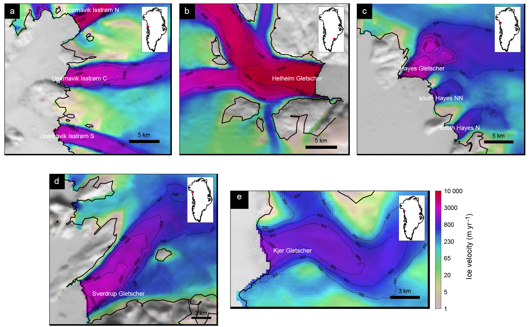
Figure 1Ice surface velocity (black contours) for study glaciers (a) Upernavik Isstrøm, (b) Hayes, (c) Helheim, (d) Sverdrup, (e) Kjer. The thick black line is the ice edge.
While all of these parameterizations have been tested on idealized or single, real-world geometries, most of them have not yet been tested on a wide range of glaciers, and some of these laws have only been implemented in 1-D flowline or vertical flowband models (Vieli and Nick, 2011). The main objective of this study is to test and compare some of these calving laws on nine different Greenland outlet glaciers using a 2-D plan-view ice sheet model. Modeling ice front dynamics in a 2-D horizontal or 3-D model has been shown to be crucial, as the complex 3-D shape of the bed topography exerts an important control on the pattern of ice front retreat, which cannot be parameterized in flowline or flowband models (Choi et al., 2017; Morlighem et al., 2016). We do not include continuum damage models and the LEFM approach in this study because these laws require individual calving events to be modeled, whereas we focus here on laws that provide an “average” calving rate, or a calving front position, without the need to track individual calving events. While these approaches remain extremely useful to derive new parameterizations, their implementation in large-scale models is not yet possible due to the level of mesh refinement required to track individual fractures.
We implement and test four different calving laws, namely the height-above-buoyancy criterion (Vieli et al., 2001), the crevasse-depth calving law (Benn et al., 2017; Otero et al., 2010), the eigencalving law (Levermann et al., 2012) and von Mises tensile stress calving law (Morlighem et al., 2016), and model calving front migration of nine tidewater glaciers of Greenland for which we have a good description of the bed topography (Morlighem et al., 2017). The glaciers of this study are three branches of Upernavik Isstrøm (UI), Helheim glacier, three sectors of Hayes glacier, Kjer, and Sverdrup glaciers (Fig. 1). Each of these four calving laws includes a calibration parameter that is manually tuned for each glacier. These parameters are assumed to be constant for each glacier. To calibrate this parameter, we first model the past 10 years (2007–2017) using each calving law and compare the modeled retreat distance to the observed retreat distance. Once a best set of parameters is found, we run the model forward with the current ocean and atmospheric forcings held constant to investigate the impact of the calving laws on forecast simulations. We discuss the differences between results obtained with different calving laws for the hindcast and forecast simulations and the implications thereof for the application of the calving laws to real glacier cases.
We use the Ice Sheet System Model (Larour et al., 2012) to implement four calving laws and to model nine glaciers. Our model relies on a Shelfy-Stream Approximation (MacAyeal, 1989; Morland and Zainuddin, 1987), which is suitable for fast outlet glaciers of Greenland (Larour et al., 2012). The mesh resolution varies from 100 m near the ice front to 1000 m inland, and the simulations have different time steps that vary between 0.72 and 7.2 days depending on the glacier in order to satisfy the Courant–Friedrichs–Lewy condition (Courant et al., 1928). We use the surface elevation and bed topography data from BedMachine Greenland version 3 (Morlighem et al., 2017). The nominal date of this dataset is 2008, which is close to our starting time of 2007. The surface mass balance (SMB) is from the regional atmospheric model RACMO2.3 (Noël et al., 2015) and is kept constant during our simulations. We invert for the basal friction to initialize the model, using ice surface velocity derived from satellite observations acquired in a similar period (2008–2009) (Rignot and Mouginot, 2012).
ISSM relies on the level set method (Bondzio et al., 2016) to track the calving front position. We define a level set function, φ, as being positive where there is no ice (inactive) and negative where there is ice (active region), and the calving front is implicitly defined as the zero contour of φ. Here, we implement two types of calving laws: EC and VM provide a calving rate, c, whereas HAB and CD provide a criterion that defines where the ice front is located. These two types of law are implemented differently within the level set framework of ISSM.
When a calving rate is provided, the level set is advected following the velocity of the ice front (vfront), defined as a function of the ice velocity vector, v, calving rate, c, and the melting rate at the calving front, :
where n is a unit normal vector that points outward from the ice.
EC defines c as proportional to strain rate along (ϵ∥) and transversal (ϵ⟂) to horizontal flow (Levermann et al., 2012):
where K is a proportionality constant that captures the material properties relevant for calving. K is the calibration parameter of this calving law.
In VM, c is assumed to be proportional to the tensile von Mises stress, , which only accounts for the tensile component of the stress in the horizontal plane:
with
where σmax is a stress threshold that is calibrated, B is the ice viscosity parameter, n=3 is Glen's exponent, and is the effective tensile strain rate defined as
where and are the two eigenvalues of the 2-D horizontal strain rate tensor (Morlighem et al., 2016). To prevent unrealistic calving rates caused by an abrupt increase in velocity upstream from the ice front, we limit the maximum calving rate to 3 km yr−1.
For HAB and CD, we proceed in two steps at each time iteration as they do not provide explicit calving rates, c. First, the ice front is advected following Eq. (1), assuming that c=0 and using the appropriate melt rate, , which simulates an advance or a retreat of the calving front without any calving event. The calving front position is then determined by examining where the condition of each law is met. The level set, φ, is explicitly set to +1 (no ice) or −1 (ice) on each vertex of our finite element mesh depending on that condition.
For HAB, the ice front thickness in excess of floatation cannot be less than the fixed height-above-buoyancy threshold, HO (Vieli et al., 2001):
where ρw and ρi are the densities of sea water and ice, respectively, and Dw is the water depth at the ice front, here represented by the bed depth below sea level. The fraction of the floatation thickness at the terminus is our calibration parameter.
For CD, the calving front is defined as where the surface crevasses reach the waterline or surface and basal crevasses join through the full glacier thickness. The depth of surface (ds) or basal (db) crevasses is estimated from the force balance between tensile stress in the along-flow direction or any direction, water pressure in the crevasse, and the lithostatic pressure:
where g is the gravitational acceleration, Hab is the height above floatation, and dw is the water height in the crevasse, which allows the crevasse to penetrate deeper (van der Veen, 1998). The water depth in the crevasse (dw) is the calibration parameter of this calving law. In this study, we use two different estimations for the crevasse opening stress, σ. First, we use the stress only in the ice-flow direction to estimate σ in which changes in direction are taken into account (Otero et al., 2010). The other estimation for σ is the largest principal component of deviatoric stress tensor to account for tensile stress in any direction (Benn et al., 2017; Todd et al., 2018). Here we use the term “CD1” (flow direction) and “CD2” (all directions), respectively, to refer to these two estimations for σ.
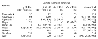
Table 1Chosen calibration parameters. The values in brackets are the range of calibration parameters that produce a qualitatively similar ice front retreat pattern to the chosen calibration parameter.
We use the frontal melt parameterization from Rignot et al. (2016) to estimate in Eq. (1). The frontal melt rate, , depends on subglacial discharge, qsg, and ocean thermal forcing, TF, defined as the difference in temperature between the potential temperature of the ocean and the freezing point of seawater, as
where h is the water depth, m−α dayα−1 ∘C−β, α=0.39, b=0.15 m day−1 ∘C−β, and β=1.18. We use ocean temperature from the Estimating the Circulation and Climate of the Ocean, Phase 2 (ECCO2) project (Rignot et al., 2012). To estimate subglacial discharge, we integrate the RACMO2.3 runoff field over the drainage basin, assuming that surface runoff is the dominant source of subglacial fresh water in summer (Rignot et al., 2016).
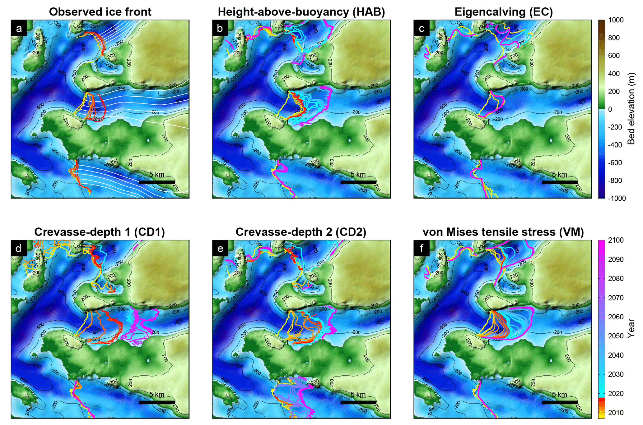
Figure 2(a) The observed ice front positions between 2007 and 2017 and (b–f) modeled ice front positions obtained with different calving laws between 2007 and 2100 overlaid on the bed topography of Upernavik Isstrøm. The white lines are the flowlines used to calculate retreat or advance distance of the ice front.
We determine each calibration parameter (Table 1) by simulating the ice front change between 2007 and 2017 and comparing the modeled pattern of retreat to observed retreat. We manually adjust these parameters for each calving law and for each basin to qualitatively best capture the observed variations in ice front position. In order to compare modeled ice front dynamics with observations, we estimate the retreat distance along five flowlines across the calving front of each glacier so that we are able to account for potential asymmetric ice front retreats. We only calculate the retreat distance between 2007 and 2017 and choose the parameters that can produce similar retreat distance for each flowline. We do not take into account the timing of the retreat or advance between 2007 and 2017 when choosing calibration parameters (Figs. S5–S7 in the Supplement). Based on our calibrated models, we run the models forward until 2100 to investigate and compare the influence of different calving parameterizations on future ice front changes. For better comparison, we keep other factors (e.g., SMB, basal friction) constant in our runs. We also keep our ocean thermal forcing (Eq. 9) the same as the last year of the hindcast simulation (2016–2017) until the end of our forecast simulations. The simulations are therefore divided into two time intervals: the hindcast period (2007–2017) that we use to calibrate the tuning parameters of the different calving laws and the forecast time period (2018–2100).
The observed and modeled ice front evolutions in our simulations are shown in Figs. 2–6. The modeled retreat distances along five flowlines are compared to observed retreat distances in Fig. 7. We first notice that, in all cases, the calving laws that model a calving rate (EC and VM) have a smoother calving front than other laws. This results from the numerical implementation of these laws in which it is only required that the advection equation of the calving front is solved, and a local post-processing step is not relied upon that may yield a more irregular shape of the calving front.
If we look at individual glaciers, Fig. 2a shows the observed pattern of retreat between 2007 and 2017 for the three branches of UI. The northern and southern branches have been rather stable over the past 10 years, but the central branch has retreated by 2.6 to 4 km. Figure 2b shows the pattern of modeled ice front position between 2007 and 2017 (warm colors) and 2017 and 2100 (cold colors) using HAB. We observe that the ice front in the central branch jumps upstream by about 2–3.5 km at the beginning of the simulation and slows down as the bed elevation increases. The ice front starts retreating again after 2017 and stops when it reaches higher ground about 5 km upstream. The modeled northern and southern branches are stable until 2017 and the northern branch retreats significantly to another ridge upstream between 2017 and 2100. The modeled ice front using EC does not match the observed pattern of ice front retreat well (Fig. 2c). This approach causes the calving front to be either remarkably stable or creates an ice front with a strongly irregular shape. Figure 2d and e present the modeled ice front evolution using the CD1 and CD2, respectively. Both models have similar ice front retreat patterns between 2007 and 2017, and they both overestimate the retreat of the central branch compared to observations (Fig. 7). In the forecast simulations, the central branch retreats more when only the flow-direction stress is considered (Fig. 2d). However, in both cases, the ice front stops retreating at the same location on a pronounced ridge. The model that relies on VM shows a gradual terminus retreat and stabilizes at the end of 2017 (Fig. 2f). After 2017, the retreat behavior is similar to the one with the height-above-buoyancy law. We observe that HAB and VM reproduce the observed changes reasonably well, although they do not capture the exact timing of the 2007–2017 retreat (Fig. 2b and f).
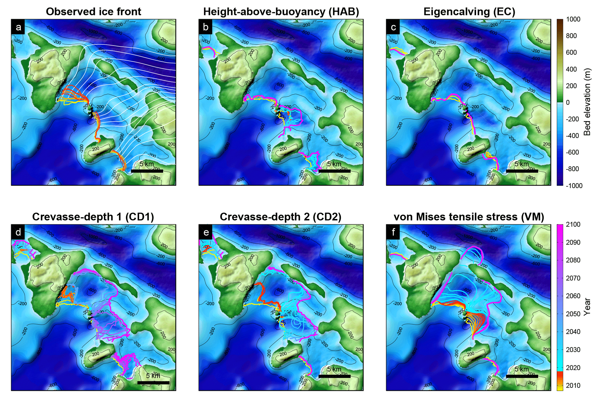
The second region of interest is Hayes glacier. Currently, the three branches of this system rest on a topographic ridge, ∼300 m below sea level, which is likely responsible for the observed stability in the position of the ice front over the past 10 years (Fig. 3a). The ice front of the northern glacier, however, retreated by up to 3 km from 2007 to 2014 and readvanced in 2016 and 2017. In this region, HAB produces a stable ice front for the northern (Hayes) and the southern sector (Hayes N), but the central sector (Hayes NN) retreats more than the observations by 0.5–0.7 km (Fig. 3b). After 2017, Hayes NN and Hayes N only retreat by a few kilometers and stabilize there until the end of the simulation. The model using EC shows very little change between 2007 and 2100 (Fig. 3c). As in the previous region, both the CD1 and CD2 show very similar results (Fig. 3d and e). In the hindcast simulation (2007–2017), both models overestimate the retreat at the western part of the northern branch (Hayes). After 2017, Hayes and Hayes NN retreat quickly by 2.2–6 km into an overdeepening in the bed topography. The final positions of the ice front derived from two crevasse-depth laws are 5 km upstream of their initial position on higher ridges further upstream. Figure 3f shows the modeled ice front evolution using VM. This model reproduces the stable ice front positions for two sectors (Hayes and Hayes N) but tends to overestimate the retreat for Hayes NN. Although, for the forecast simulation, VM results in more retreat than obtained with other laws for Hayes, the ice front ends up resting on the same ridges as the ones based on the crevasse-depth laws.
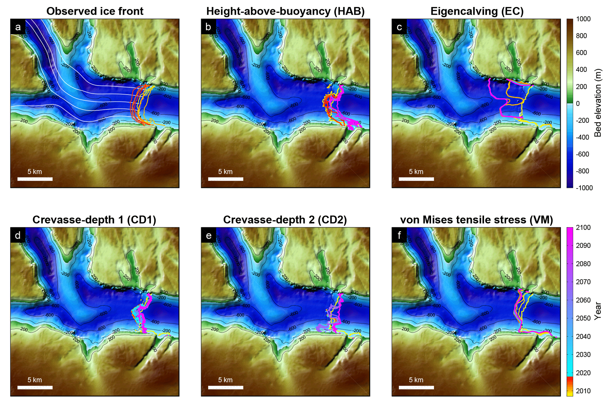

Figure 4a shows the observed ice front pattern for Helheim glacier. Since 2007, this glacier has shown a stable ice front evolution, retreating or advancing only by a few kilometers over the past 10 years (Cook et al., 2014). All calving parameterizations, except for EC, result in a stable or a little advanced ice front pattern (Fig. 4b–f), and only the VM model reproduces the observed retreat distance from 2007 to 2017 for this region reasonably well (Fig. 7g), although it never readvances. The other calving laws do not capture the observed retreat distance or the shape of ice front properly with our ocean parameterization. In the forecast simulations, all model results show an advance or stable pattern of ice front evolutions at the end of 2100. The model with EC results in a significantly different shape of ice front compared to other models (Fig. 4c).
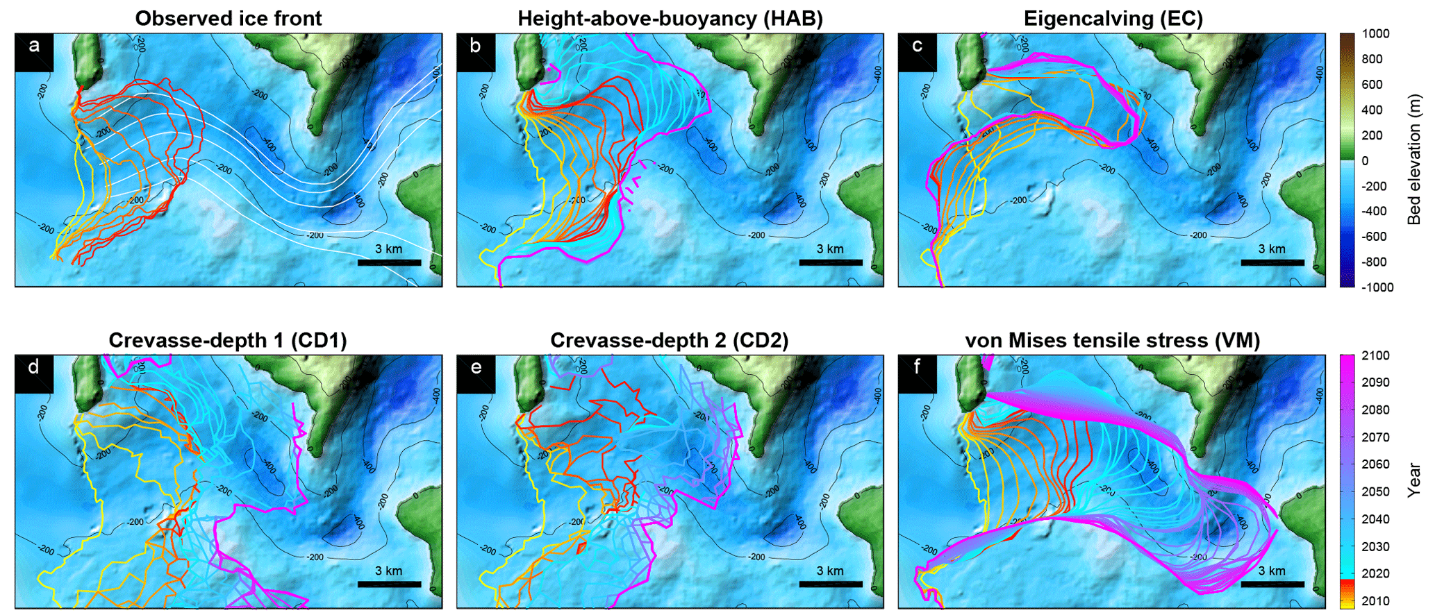
From 2007 to 2014, the mean terminus position of Sverdrup glacier (Fig. 5a) has been around a small ridge ∼300 m high. In 2014, the glacier was dislodged from its sill and the glacier started to retreat. The models with HAB and EC show that the ice front jumps to a similar location to the 2017 observed ice front (Fig. 5b and c). The glacier does not retreat much after 2017 in these two models. The two CDs tend to produce more retreat than other parameterizations after the ice front is dislodged from the ridge (Fig. 5d and e). The ice front retreat, after 2017, starts slowing down near another ridge 9 km upstream and the glacier stabilizes there until 2100. Only VM captures the timing of the retreat reasonably right (Fig. 5f). After 2017, the forecast simulation shows that ice front retreats up to 4.5 km before slowing down at the second ridge upstream. The ice front then retreats past this ridge quickly and keeps retreating until it reaches a bed above sea level further upstream, where the retreat stops.
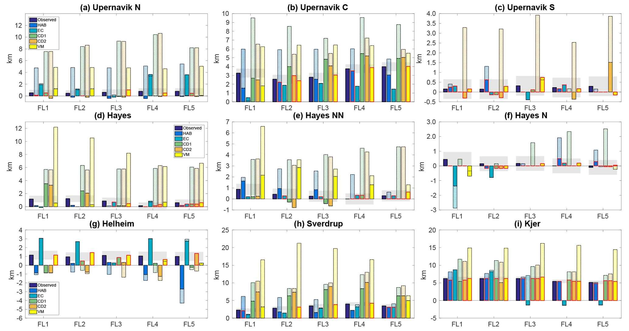
Figure 7Modeled retreat distances (with respect to the calving front initial position in 2007) for different calving laws compared to observed retreat distance for nine study glaciers. The retreat distances between 2007 and 2017 from each calving law are shown as bar solid colors. The hatched bars are the retreated distances in 2100 for each calving law. Shaded areas represent the range of 500 m from the 2017 observed retreat, and the modeled retreats that fall into this range are shown with the red edge.
The ice front of Kjer glacier retreated continuously between 2007 and 2017 (Fig. 6a). All calving parameterizations, except for EC, simulate the observed retreat well (Figs. 6b–f and 7i). The forecast simulations, however, show different retreat patterns. HAB shows relatively less retreat than other models (Fig. 6b). The calving front slows down and stabilizes at the location where the direction of the trough changes. The calving front from two crevasse-depth parameterizations retreats past this pinning point and stops retreating at the next pinning point where the small ridge is located (Fig. 6d and e). In the model with VM, the retreat rate slows down near this ridge as well. The ice front, however, keeps retreating beyond this ridge and stabilizes on another ridge further upstream (Fig. 6f).
Our results show that different calving laws produce different patterns of ice front retreat in both timing and magnitude, despite equal climatic forcing. In the hindcast simulations, we calculate the modeled retreat distance from 2007 to 2017 for a total of 45 flowlines from our study glaciers to investigate which calving law, with the best tuning parameter, better captures the observed ice front changes (Fig. 7). We find that overall, VM captures the observed retreat better than other calving laws. For 67 % (30 out of 45) of these flowlines, VM reproduces the retreat distance within 500 m from the observations, which we assume to be a reasonable range based on the seasonal variability of ice fronts, error in observations, and model resolution (Bevan et al., 2012; Howat et al., 2010). With HAB, the modeled retreat distance is within 500 m of the observed retreat distance for 53 % of the flowlines, while CD1 and CD2 capture the retreat for 51 % and 40 % of the the flowlines. EC reproduces only 31 % of the retreat that falls into the 500 m range.
EC was designed to model calving of large-scale floating shelves by including strain rates along and across ice flow (Levermann et al., 2012). Our results show that it does not work well in the case of Greenland fjords because these glaciers flow along narrow and almost parallel valleys. The transversal strain rate, ϵ⟂, is small and noisy in these valleys, leading to a significantly different pattern of ice front changes with either a remarkably stable (e.g., Fig. 3c) or some complex shape of the modeled ice front (e.g., Figs. 2c, 4c). The forecast simulations with this calving law also show different retreat patterns compared to other calving laws. While this calving law may be appropriate in the case of unconfined ice shelves, we do not recommend using this calving law for Greenland glaciers.
The two crevasse-depth calving laws are very similar in terms of the ice front retreat patterns they produce. For the regions of fast flow, the maximum principal strain rate is almost the same as the along-flow strain rate, which leads to a similar amount of stress for opening crevasses. We note that for almost all of the glaciers that match the observed retreat, the model is very sensitive to the water depth in crevasses, the calibration parameter, for both laws (Table 1). Even a 1 m increase in water depth significantly changes the calving rate, and thus the entire glacier dynamics. This behavior has been noticed in other modeling studies (Cook et al., 2012; Otero et al., 2017). Only one glacier (Hayes N) allows the water depth to be changed by up to ∼18 m and still reproduces the observed ice front pattern. One reason why CDs do not capture the rate of retreat well in the hindcast simulations might also be this high sensitivity to water depth in crevasses. Models relying on this law should be taken with caution because it is hard to constrain the water depth in crevasses. The water depth in crevasses is certainly different from one year to another, and can be significantly affected by changes in surface melting and the hydrology of glacier surfaces for the forecast simulations (Nick et al., 2013). Todd et al. (2018) applied a CD calving law with a 3-D full Stokes model and were able to reproduce the seasonal calving variability of Store Glacier without any tuning of water depth in crevasses. For our study glaciers, however, tuning the water depth was necessary to reproduce the observed ice front changes (Figs. S1–S4). This either shows that this calving law works well for Store but not for other glaciers without the tuning process, or that full 3-D stresses are required to model calving. Further studies need to investigate the stresses from different models and their relationships with water depth in crevasses.
The model results with HAB indicate that this calving law reproduces the final position of observed calving front well for some glaciers, but does not capture continuous retreat patterns and the timing of retreat between 2007 and 2017. The ice front generally tends to jump to its final position. This may be due to the fact that we keep the height above floatation fraction (q) constant during our simulations. This constant fraction value also explains a relatively limited retreat compared to other calving laws for the forecast simulations. The sensitivity of the model to the parameter q is different for every glacier (Table 1). The glaciers with an ice front that is in shallow water (e.g., Hayes N, Kjer) are less sensitive to the choice of q than the ones with a deeper ice front. A wide range of grounding conditions in the study glaciers also explains the wide range of the parameter q between different glaciers. Because determining q is empirical and buoyancy conditions may change through time, this calving law becomes less reliable than other physics-based calving laws for the forecast simulations. Another disadvantage of this law is that it does not allow for the formation of a floating extension, and cannot be applied to ice shelves.
All calving laws implemented in this study rely on parameter tuning for each glacier in order to match observations. However, this tuning process makes it difficult to apply any of these calving laws to glaciers for which we have no observations of ice front change, and it is not clear whether these parameters should be held constant in future simulations or whether they may change. In particular, when the parameters span a wide range between different glaciers, as in HAB or EC, it is hard to constrain these parameters for forecast simulations. Model simulations with these calving laws should be taken with caution.
Our results for forecast simulations suggest that ice front retreat strongly depends on the bed topography. Although different calving laws do not always have the same final positions, the extent of glacier retreat shows a similar pattern: topographic ridges slow down or/and stop the retreat, and retrograde slopes accelerate the retreat, which has been shown in several studies (Choi et al., 2017; Morlighem et al., 2016). Whether the glaciers continue to retreat beyond these ridges depends on the calving law used and may also depend on the choice of tuning parameters. For the forecast simulations, it is not clear whether the tuning coefficients of the calving laws should be kept constant, as we did here. Some parameters potentially vary depending on future changes in external climate forcings or ice properties. These changes may affect the final locations where glaciers eventually stabilize. However, the bed topography still plays a crucial role in determining stable positions of ice fronts and the general pattern of retreat before the glaciers stabilize.
The results for Helheim glacier are very similar for all calving laws, and none of them captures the pattern of ice front migration perfectly. In the forecast simulations, the modeled ice front slightly advances until 2100 for all calving laws. This ice front advance is mostly caused by the ocean thermal forcing data used in the forecast simulations. The thermal forcing has been slightly decreasing after 2012 and a relatively cold water is applied to our forecast simulations, which leads to a similar advance of ice front for all calving law simulations. However, according to the bed topography of this region, this glacier might potentially retreat upstream if the ocean temperature increases, which may trigger more frequent calving events.
Ocean forcing is one of the limitations of this study: the frontal melt rate is simply parameterized. The ocean parameterization does not take into account ocean circulation within the fjords, which could cause localized melt higher or lower than the parameterization. We need to account for these ocean processes that may affect melt rate and could potentially vary the retreat rate of ice front. We also assume that the calving front remains vertical and the melt is applied uniformly along the calving face (Choi et al., 2017). Future studies should include more detailed ocean physics and coupling to better calibrate our calving laws and improve results.
Based on our results, we recommend using the von Mises stress calving law (VM) for modeling centennial changes in Greenland tidewater glaciers within a 2-D plan-view or 3-D model. This calving law captures the observed pattern of retreat and rate of retreat better than other calving laws, and does allow for the formation of a floating extension. VM does not, however, necessarily capture specific modes of calving as it is only based on horizontal tensile stresses, which may be a reason why it does not always capture the pattern of ice front migration perfectly. The strong correlation between calving rate and ice velocity produces reasonable calving rates (Fig. S8) but whether these relationships hold for forecast simulations needs further investigation. Another disadvantage of this law is that it strongly depends on the stress threshold, σmax, that needs to be calibrated. Some modeled glaciers (e.g., Helheim, Sverdrup, Kjer) are very sensitive to σmax, in which case a ∼50 kPa change significantly affects the calving dynamics of these glaciers (Table 1). As a result, the modeled ice front dynamics is dependent on this one single value that we keep constant through time and uniform in space, which adds uncertainty to model projections. It is therefore critical to further validate the stress threshold and improve this law by accounting for other modes of calving or to develop new parameterizations. Current research based on discrete element models (Benn et al., 2017) or on damage mechanics (Duddu et al., 2013) may help the community derive these new parameterizations.
We test and compare four calving laws by modeling nine tidewater glaciers of Greenland with a 2-D plan-view ice sheet model. We implement the height-above-buoyancy criterion, eigencalving law, crevasse-depth calving laws, and von Mises stress calving parameterization in order to investigate how these different calving laws simulate observed front positions and affect forecast simulations. Our simulations show that the von Mises stress calving law reproduced observations better than other calving laws although it may not capture all the physics involved in calving events. Other calving laws do not capture the pattern or pace of observed retreat as well as the VM. In forecast simulations, the pattern of ice front retreat is somewhat similar for most calving laws because of the strong control of the bed topography on ice front dynamics. Based on our results, we recommend using the tensile von Mises stress calving law, but new parameterizations should be derived in order to better capture and understand the complex processes involved in calving dynamics. It is not clear, however, whether these recommendations would apply to Antarctic ice shelves. These ice shelves calve large tabular icebergs that may be governed by different physics.
The data used in this study are freely available at the National Snow and Ice Data Center, or upon request to the authors. The ISSM is open source and is available at http://issm.jpl.nasa.gov (Version 4.13, released on 10 May 2018).
The supplement related to this article is available online at: https://doi.org/10.5194/tc-12-3735-2018-supplement.
YC and MM designed the experiments. YC conducted the numerical modeling simulations with help from MM and JHB. MW provided the data related to ocean melt rates. YC wrote the first version of the manuscript with inputs from MM, JHB, and MW.
The authors declare that they have no conflict of interest.
We would like to thank the editor, Olivier Gagliardini, for his constructive comments after the
initial submission of this manuscript. This work was performed at the University of California
Irvine under a contract with the National Science Foundation's ARCSS program (no. 1504230), the
National Aeronautics and Space Administration, Cryospheric Sciences Program (no. NNX15AD55G), and
the NASA Earth and Space Science Fellowship Program (no. 80NSSC17K0409).
Edited by: Olivier Gagliardini
Reviewed by: Doug Benn and Jeremy Bassis
Albrecht, T. and Levermann, A.: Fracture-induced softening for large-scale ice dynamics, The Cryosphere, 8, 587–605, https://doi.org/10.5194/tc-8-587-2014, 2014. a
Benn, D. I., Warren, C. R., and Mottram, R. H.: Calving processes and the dynamics of calving glaciers, Earth Sci. Rev., 82, 143–179, https://doi.org/10.1016/j.earscirev.2007.02.002, 2007. a, b
Benn, D. I., Cowton, T., Todd, J., and Luckman, A.: Glacier Calving in Greenland, Curr. Clim. Change Rep., 3, 282–290, https://doi.org/10.1007/s40641-017-0070-1, 2017. a, b, c
Bevan, S. L., Luckman, A. J., and Murray, T.: Glacier dynamics over the last quarter of a century at Helheim, Kangerdlugssuaq and 14 other major Greenland outlet glaciers, The Cryosphere, 6, 923–937, https://doi.org/10.5194/tc-6-923-2012, 2012. a
Bondzio, J. H., Seroussi, H., Morlighem, M., Kleiner, T., Rückamp, M., Humbert, A., and Larour, E. Y.: Modelling calving front dynamics using a level-set method: application to Jakobshavn Isbræ, West Greenland, The Cryosphere, 10, 497–510, https://doi.org/10.5194/tc-10-497-2016, 2016. a
Bondzio, J. H., Morlighem, M., Seroussi, H., Kleiner, T., Ruckamp, M., Mouginot, J., Moon, T., Larour, E., and Humbert, A.: The mechanisms behind Jakobshavn Isbræ's acceleration and mass loss: A 3-D thermomechanical model study, Geophys. Res. Lett., 44, 6252–6260, https://doi.org/10.1002/2017GL073309, 2017. a
Brown, C., Meier, M., and Post, A.: Calving speed of Alaska tidewater Glaciers, with application to Columbia Glacier, Alaska, U.S. Geological Survey Professional Paper 1258–C., US Gov. Print. Off., Washington, D.C., 13 pp., 1982. a
Choi, Y., Morlighem, M., Rignot, E., Mouginot, J., and Wood, M.: Modeling the response of Nioghalvfjerdsfjorden and Zachariae Isstrøm glaciers, Greenland, to ocean forcing over the next century, Geophys. Res. Lett., 44, 11071–11079, https://doi.org/10.1002/2017GL075174, 2017. a, b, c, d, e
Cook, S., Zwinger, T., Rutt, I. C., O'Neel, S., and Murray, T.: Testing the effect of water in crevasses on a physically based calving model, Ann. Glaciol., 53, 90–96, https://doi.org/10.3189/2012AoG60A107, 2012. a
Cook, S., Rutt, I. C., Murray, T., Luckman, A., Zwinger, T., Selmes, N., Goldsack, A., and James, T. D.: Modelling environmental influences on calving at Helheim Glacier in eastern Greenland, The Cryosphere, 8, 827–841, https://doi.org/10.5194/tc-8-827-2014, 2014. a
Courant, R., Friedrichs, K., and Lewy, H.: Über die partiellen Differenzengleichungen der mathematischen Physik, Mathematische Annalen, 100, 32–74, https://doi.org/10.1007/BF01448839, 1928. a
Cuffey, K. and Paterson, W. S. B.: The Physics of Glaciers, 4th edn., Elsevier, Oxford, UK, 2010. a
Duddu, R., Bassis, J. N., and Waisman, H.: A numerical investigation of surface crevasse propagation in glaciers using nonlocal continuum damage mechanics, Geophys. Res. Lett., 40, 3064–3068, https://doi.org/10.1002/grl.50602, 2013. a, b
Gagliardini, O., Durand, G., Zwinger, T., Hindmarsh, R. C. A., and Le Meur, E.: Coupling of ice-shelf melting and buttressing is a key process in ice-sheets dynamics, Geophys. Res. Lett., 37, 1–5, https://doi.org/10.1029/2010GL043334, 2010. a
Howat, I. M., Joughin, I., Fahnestock, M., Smith, B. E., and Scambos, T. A.: Synchronous retreat and acceleration of southeast Greenland outlet glaciers 2000–06: ice dynamics and coupling to climate, J. Glaciol., 54, 646–660, 2008. a
Howat, I. M., Box, J. E., Ahn, Y., Herrington, A., and McFadden, E. M.: Seasonal variability in the dynamics of marine-terminating outlet glaciers in Greenland, J. Glaciol., 56, 601–613, https://doi.org/10.3189/002214310793146232, 2010. a
Krug, J., Weiss, J., Gagliardini, O., and Durand, G.: Combining damage and fracture mechanics to model calving, The Cryosphere, 8, 2101–2117, https://doi.org/10.5194/tc-8-2101-2014, 2014. a
Larour, E., Seroussi, H., Morlighem, M., and Rignot, E.: Continental scale, high order, high spatial resolution, ice sheet modeling using the Ice Sheet System Model (ISSM), J. Geophys. Res., 117, 1–20, https://doi.org/10.1029/2011JF002140, 2012. a, b
Levermann, A., Albrecht, T., Winkelmann, R., Martin, M. A., Haseloff, M., and Joughin, I.: Kinematic first-order calving law implies potential for abrupt ice-shelf retreat, The Cryosphere, 6, 273–286, https://doi.org/10.5194/tc-6-273-2012, 2012. a, b, c, d
MacAyeal, D. R.: Large-scale ice flow over a viscous basal sediment: Theory and application to Ice Stream B, Antarctica, J. Geophys. Res., 94, 4071–4087, 1989. a
Moon, T. and Joughin, I.: Changes in ice front position on Greenland's outlet glaciers from 1992 to 2007, J. Geophys. Res., 113, 1–10, https://doi.org/10.1029/2007JF000927, 2008. a
Morland, L. and Zainuddin, R.: Plane and radial ice-shelf flow with prescribed temperature profile, in: Dynamics of the West Antarctica Ice Sheet, edited by: van der Veen, C. J. and Oerlemans, J., Proceedings of a Workshop held in Utrecht, 6–8 May 1985, D. Rediel Publishing Company, Dordrecht, the Netherlands, 117–140, 1987. a
Morlighem, M., Bondzio, J., Seroussi, H., Rignot, E., Larour, E., Humbert, A., and Rebuffi, S.-A.: Modeling of Store Gletscher's calving dynamics, West Greenland, in response to ocean thermal forcing, Geophys. Res. Lett., 43, 2659–2666, https://doi.org/10.1002/2016GL067695, 2016. a, b, c, d, e, f
Morlighem, M., Williams, C. N., Rignot, E., An, L., Arndt, J. E., Bamber, J. L., Catania, G., Chauché, N., Dowdeswell, J. A., Dorschel, B., Fenty, I., Hogan, K., Howat, I., Hubbard, A., Jakobsson, M., Jordan, T. M., Kjeldsen, K. K., Millan, R., Mayer, L., Mouginot, J., Noël, B. P. Y., O'Cofaigh, C., Palmer, S., Rysgaard, S., Seroussi, H., Siegert, M. J., Slabon, P., Straneo, F., van den Broeke, M. R., Weinrebe, W., Wood, M., and Zinglersen, K. B.: BedMachine v3: Complete bed topography and ocean bathymetry mapping of Greenland from multi-beam echo sounding combined with mass conservation, Geophys. Res. Lett., 44, 11051–11061, https://doi.org/10.1002/2017GL074954, 2017. a, b
Nick, F. M., van der Veen, C. J., Vieli, A., and Benn, D. I.: A physically based calving model applied to marine outlet glaciers and implications for the glacier dynamics, J. Glaciol., 56, 781–794, 2010. a, b
Nick, F. M., Luckman, A., Vieli, A., Van Der Veen, C., Van As, D., Van De Wal, R., Pattyn, F., Hubbard, A., and Floricioiu, D.: The response of Petermann Glacier, Greenland, to large calving events, and its future stability in the context of atmospheric and oceanic warming, J. Glaciol., 58, 229–239, 2012. a
Nick, F. M., Vieli, A., Andersen, M. L., Joughin, I., Payne, A., Edwards, T. L., Pattyn, F., and van de Wal, R. S. W.: Future sea-level rise from Greenland's main outlet glaciers in a warming climate, Nature, 497, 235–238, https://doi.org/10.1038/nature12068, 2013. a, b
Noël, B., van de Berg, W. J., van Meijgaard, E., Kuipers Munneke, P., van de Wal, R. S. W., and van den Broeke, M. R.: Evaluation of the updated regional climate model RACMO2.3: summer snowfall impact on the Greenland Ice Sheet, The Cryosphere, 9, 1831–1844, https://doi.org/10.5194/tc-9-1831-2015, 2015. a
Otero, J., Navarro, F., Martin, C., Cuadrado, M., and Corcuera, M.: A three-dimensional calving model: numerical experiments on Johnsons Glacier, Livingston Island, Antarctica, J. Glaciol., 56, 200–214, 2010. a, b, c
Otero, J., Navarro, F. J., Lapazaran, J. J., Welty, E., Puczko, D., and Finkelnburg, R.: Modeling the Controls on the Front Position of a Tidewater Glacier in Svalbard, Front. Earth Sci., 5, 2, https://doi.org/10.3389/feart.2017.00029, 2017. a
Pfeffer, W., Dyurgerov, M., Kaplan, M., Dwyer, J., Sassolas, C., Jennings, A., Raup, B., and Manley, W.: Numerical modeling of late Glacial Laurentide advance of ice across Hudson Strait: Insights into terrestrial and marine geology, mass balance, and calving flux, Paleoceanography, 12, 97–110, https://doi.org/10.1029/96PA03065, 1997. a
Rignot, E. and Mouginot, J.: Ice flow in Greenland for the International Polar Year 2008–2009, Geophys. Res. Lett., 39, L11501, https://doi.org/10.1029/2012GL051634, 2012. a
Rignot, E., Fenty, I., Menemenlis, D., and Xu, Y.: Spreading of warm ocean waters around Greenland as a possible cause for glacier acceleration, Ann. Glaciol., 53, 257–266, https://doi.org/10.3189/2012AoG60A136, 2012. a
Rignot, E., Jacobs, S., Mouginot, J., and Scheuchl, B.: Ice shelf melting around Antarctica, Science, 341, 266–270, https://doi.org/10.1126/science.1235798, 2013. a
Rignot, E., Xu, Y., Menemenlis, D., Mouginot, J., Scheuchl, B., Li, X., Morlighem, M., Seroussi, H., v. den Broeke, M., Fenty, I., Cai, C., An, L., and de Fleurian, B.: Modeling of ocean-induced ice melt rates of five West Greenland glaciers over the past two decades, Geophys. Res. Lett., 43, 6374–6382, https://doi.org/10.1002/2016GL068784, 2016. a, b
Todd, J., Christoffersen, P., Zwinger, T., Raback, P., Chauché, N., Benn, D., Luckman, A., Ryan, J., Toberg, N., Slater, D., and Hubbard, A.: A Full-Stokes 3-D Calving Model Applied to a Large Greenlandic Glacier, J. Geophys. Res.-Earth, 123, 410–432, https://doi.org/10.1002/2017JF004349, 2018. a, b
van der Veen, C.: Fracture mechanics approach to penetration of surface crevasses on glaciers, Cold Reg. Sci. Technol., 27, 31–47, 1998. a
van der Veen, C.: Calving glaciers, Prog. Phys. Geogr., 26, 96–122, https://doi.org/10.1191/0309133302pp327ra, 2002. a
Vieli, A. and Nick, F.: Understanding and modelling rapid dynamic changes of tidewater outlet glaciers: Issues and implications, Surv. Geophys., 32, 437–458, 2011. a
Vieli, A., Funk, M., and Blatter, H.: Flow dynamics of tidewater glaciers: a numerical modelling approach, J. Glaciol., 47, 595–606, https://doi.org/10.3189/172756501781831747, 2001. a, b, c
Vieli, A., Jania, J., and Kolondra, L.: The retreat of a tidewater glacier: observations and model calculations on Hansbreen, Spitsbergen, J. Glaciol., 48, 592–600, https://doi.org/10.3189/172756502781831089, 2002. a
Yu, H., Rignot, E., Morlighem, M., and Seroussi, H.: Iceberg calving of Thwaites Glacier, West Antarctica: full-Stokes modeling combined with linear elastic fracture mechanics, The Cryosphere, 11, 1283–1296, https://doi.org/10.5194/tc-11-1283-2017, 2017. a