the Creative Commons Attribution 4.0 License.
the Creative Commons Attribution 4.0 License.
 | 28 Feb 2018
Calving relation for tidewater glaciers based on detailed stress field analysis
Rémy Mercenier
Martin P. Lüthi
Andreas Vieli
Ocean-terminating glaciers in Arctic regions have undergone rapid dynamic changes in recent years, which have been related to a dramatic increase in calving rates. Iceberg calving is a dynamical process strongly influenced by the geometry at the terminus of tidewater glaciers. We investigate the effect of varying water level, calving front slope and basal sliding on the state of stress and flow regime for an idealized grounded ocean-terminating glacier and scale these results with ice thickness and velocity. Results show that water depth and calving front slope strongly affect the stress state while the effect from spatially uniform variations in basal sliding is much smaller. An increased relative water level or a reclining calving front slope strongly decrease the stresses and velocities in the vicinity of the terminus and hence have a stabilizing effect on the calving front. We find that surface stress magnitude and distribution for simple geometries are determined solely by the water depth relative to ice thickness. Based on this scaled relationship for the stress peak at the surface, and assuming a critical stress for damage initiation, we propose a simple and new parametrization for calving rates for grounded tidewater glaciers that is calibrated with observations.


Many ocean-terminating glaciers in the Arctic are currently undergoing rapid retreat, thinning and strong acceleration in flow. These dynamic mass losses contribute to about half of the Greenland ice sheet's contribution to sea level rise (van den Broeke et al., 2009) and are expected to further increase in the future (Nick et al., 2013). The mechanism of iceberg calving is thereby at the heart of these rapid dynamic changes of ocean-terminating glaciers. However, the understanding of the involved processes and the capability of predictive flow models to represent calving are limited (Straneo et al., 2013; Vieli and Nick, 2011).
Tidewater glacier evolution is the result of an interplay between mass flux from upstream and the rate and size of calving events (Post et al., 2011). Both processes are strongly influenced by the geometry of the glacier surface, the glacier bed and the bathymetry of the proglacial fjord (Nick et al., 2009) as well as external forcings such as submarine melt due to heat advection by ocean currents (Carr et al., 2013; Howat et al., 2010; Motyka et al., 2013; Straneo and Heimbach, 2013; Straneo et al., 2013) or changes in ice mélange (Amundson et al., 2010; Joughin et al., 2008).
Iceberg calving is a dynamical process of material failure which occurs when the local stress field in the vicinity of the calving front exceeds the fracture strength of ice, driving the formation and propagation of cracks and eventually leading to the detachment of a block of ice from the glacier front. The local geometry and water level at the terminus determine the stress field and thereby the fracture processes and the geometry evolution. Further, buoyancy forces of submerged ice and erosion from subaqueous melt are expected to enhance near-terminus stress intensity and hence calving rates, while a reclining terminus should reduce extensional stresses.
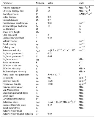
Table 1Model parameters, notations, units and values for constant parameters.
Several empirical and semi-empirical parametrizations of the calving rate for different terminus geometries have been proposed. A simple empirical relationship of linearly increasing calving rate with water depth, based on observations of tidewater glaciers in Alaska, has been established, used and extended for different regions (Benn et al., 2007b; Brown et al., 1982). This approach only depends on the local water depth at the terminus only and is not process-based, and it is therefore independent of glacier geometry and dynamics (Vieli et al., 2001). In contrast, the flotation calving criterion, proposed by Van der Veen (1996) and modified by Vieli et al. (2001), determines the position of the terminus by calving away all ice that is close to flotation. In this approach the calving rate is an emergent quantity resulting from ice flow dynamics. Benn et al. (2007a, b) introduced a physics-based approach by setting the terminus position at the location where crevasses penetrate below the water level. The crevasse depth is computed using the Nye (1957) theory, which relies on the equilibrium between longitudinal stretching and overburden stress of the ice. This dynamic approach for calving allowed for successful reproduction of calving front variations of ocean-terminating glaciers in Greenland and Antarctica (Cook et al., 2014; Nick et al., 2010, 2013; Otero et al., 2010, 2017). Although the crevasse depth model can be calibrated to observations (Lea et al., 2014), it lacks validation with field observations and is based on a snapshot of the stress balance, neglecting the pre-existence of cracks and their effect on the stress state of the glacier (Krug et al., 2014). A recent, more sophisticated approach by Benn et al. (2017) predicts calving positions based on the maximum principal stress distribution and accounts for the effect of water pressure in the submerged parts of the glacier front by combination of a continuum flow model with a discrete element model to simulate calving events.
For near-vertical calving fronts, the main driver for calving is the horizontal deviatoric stress in the vicinity of the laterally confined calving front. Its magnitude can be estimated from the difference of vertically integrated hydrostatic pressure within the ice and of ocean water at the calving front (Cuffey and Paterson, 2010). The resulting extensional stress within the ice depends on the ice thickness H and the water depth Hw at the calving front:
where ρi,ρw and are the ice density, water density and relative water depth (Table 1). This equation illustrates the square dependence of the horizontal extensional stress on relative water level at the terminus. However, it should be noted that this vertically integrated stress is not representative for the stress state near the surface of the terminus, and such a “depth-averaged” longitudinal stress may be inaccurate as bending stresses are neglected.
Using the above longitudinal stress at the front, the maximum height for which a grounded glacier with a dry calving front can sustain a stable vertical front is approximately 110 m when crevasse depth is computed according to the Nye (1957) theory and 221 m when the ice is considered as undamaged and without crevasses (Bassis and Walker, 2012). However, the presence of water along the calving front influences this maximum stable height, as an increase of water depth for a constant ice thickness reduces the stresses and hence tends to increase the stability of the glacier front. Thus, a thicker glacier must terminate in deeper water in order for its calving front not to exceed a certain stress limit and to remain stable (Bassis and Walker, 2012).
Calving termini can also be over-steepened by melt undercutting, which leads to higher stress intensities (Hanson and Hooke, 2000) and may facilitate calving (Benn et al., 2017). Ice flow model results (Hanson and Hooke, 2000) suggest that an increase of water depth leads to a higher rate of over-steepening development at the calving front and thus an increase of calving activity. However, model results seem to indicate that melt undercutting does not significantly affect calving rates (Cook et al., 2014; Krug et al., 2015), while other studies suggest that calving rates are strongly related to melt undercutting for some arctic glaciers (Cowton et al., 2016; Luckman et al., 2015; Petlicki et al., 2015). Conversely, a calving front inclined towards the inland is expected to be more stable than a vertical cliff.
The state of stress near the calving front is determined by ice geometry and water depth and controls the intensity and location of material degradation processes. Material creep and fracture processes in turn change the geometry of the glacier front. Observations and theoretical considerations indicate a tendency of increasing relative water level with increasing thickness (Bassis and Walker, 2012). This implies that thick glaciers approach flotation at their front but for shallow water depth the bounds on stress, and hence cliff geometry, are less well constrained.
The relationship between water depth, stress state, front geometry and related calving type is well illustrated at the example of Eqip Sermia, a medium-sized ocean-terminating outlet glacier on the West Greenland coast. Figure 1 shows that this glacier is characterized by two distinct calving front lobes with contrasting geometries: the grounded northern lobe exhibits a 200 m high inclined calving face with slope angles exceeding 45∘ while the southern lobe features a vertical ice cliff of ∼50 m freeboard with a water depth of ∼100 m (Lüthi et al., 2016). These substantially different geometries lead to distinct velocity and stress regimes in the proximity of the calving front which also determine the type of calving. The high, grounded, inclined northern cliff collapses at timescales of weeks, releasing large ice masses of up to 106 m3 and generating 50 m tsunami waves (Lüthi and Vieli, 2016). In contrast, the southern part of the front calves smaller volumes of ice at intervals of several hours.
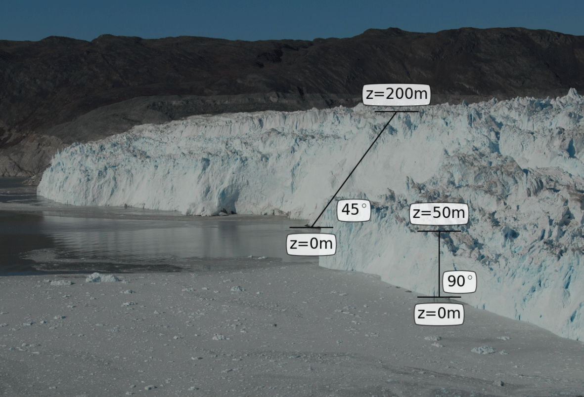
Figure 1Calving front of Eqip Sermia glacier in July 2016. The boxes in the picture describe the geometrical properties of the two distinct parts of the calving front.
Motivated partly by the case of contrasting calving front geometries at Eqip Sermia, the aim of this study is to better understand the detailed flow and stress regimes in the vicinity of the calving front of tidewater glaciers, including those that are far from flotation. Using a numerical model that solves the full equations for ice flow, we investigate the sensitivity to variations in front thickness and slope, the water depth and the strength of the coupling to the bed which results from sliding processes. We perform these model experiments on idealized geometries of grounded glacier termini and succeed to explicitly express the results as function of relative water depth.
Based on these model results, we derive a novel parametrization of calving rate that is calibrated with observations from Arctic tidewater glaciers. This parametrization only requires the relative water level and is based on a fit to the modeled stress field at the surface and an isotropic damage evolution relation.
2.1 Ice flow model and rheology
We used the finite-element library libMesh (Kirk et al., 2006) to implement the Stokes equations for continuum momentum and mass conservation:
where σ is the Cauchy stress tensor, ρi the ice density, g the gravitational force vector and u the velocity vector. As we assume ice to be incompressible and isotropic, the Cauchy stress tensor can be decomposed into an isotropic and a deviatoric part σ′:
where is the isotropic mean stress and I the identity matrix. The ice rheology is described as viscous power-law fluid (Glen's flow law), linking the deviatoric stress tensor σ′ to the strain rate tensor :
The effective shear viscosity η is defined as
where is the effective strain rate, A the fluidity parameter, n=3 the power-law exponent and κε is a finite strain rate parameter included to avoid infinite viscosity at low stresses (Greve and Blatter, 2009).
The model domain was discretized with second-order nine-node quadrangle elements with Galerkin weighting. Model variables are approximated with a second-order approximation for the velocities u and w and a first-order approximation for the mean stress σm (forming a LBB-stable set). The accuracy of the solution was improved with adaptive mesh refinement near the calving front. The Stokes equations with the nonlinear rheology were solved with the PETSc nonlinear solver SNES to a relative accuracy of 10−4 (Balay et al., 2008).
2.2 Model geometry and scaling
We used a two-dimensional version of the model to conduct the geometrical tests, as illustrated in Fig. 2. The geometry is defined in a Cartesian coordinate system with horizontal axis x and vertical axis z with origin at sea level at the calving front (where x=0). The ice moves from right to left. The idealized glacier geometry used in all model experiments consists of a block of ice resting on a flat bed with a characteristic length L=2000 m and a characteristic ice thickness H=200 m. The domain was discretized with 20 elements in the vertical and 200 elements in the horizontal which, after mesh refinement, led to a spatial resolution of 2.5 m in the terminus area.
All numerical results are scalable with reference values for ice thickness Href and overburden stress σref and are therefore independent of the geometrical extent. This validity of the scaling was tested by running the model for different ice thicknesses, which recovered identical flow and stress results. The velocity scale uref was chosen as the vertical surface velocity caused by uniaxial confined compression in pure shear of an ice block under its own weight (Cuffey and Paterson, 2010):
The coordinates and the water depth at the calving front Hw are scaled by the ice thickness Href:
All stress and velocity components are scaled according to
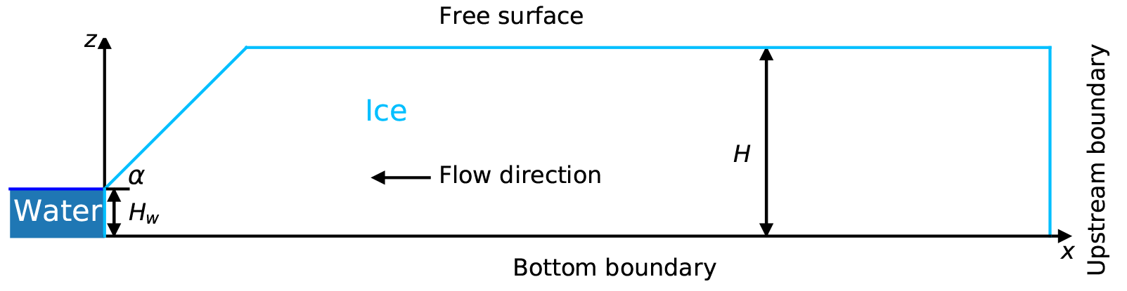
Figure 2Geometry of the idealized grounded glacier. α is the slope angle of the calving front above the vertical cliff.
2.3 Boundary conditions
The upper surface of the glacier was described as a traction-free surface boundary. Basal motion was parametrized with a slipperiness coefficient C, which relates the basal velocity ub with basal shear stress τb (Gudmundsson and Raymond, 2008; Ryser et al., 2014):
This boundary condition was implemented as a two-element layer with constant viscosity , which was added at the bottom of the model domain representing the glacier. At the lower boundary of this “sediment layer”, a Dirichlet boundary condition with zero velocity () was imposed. A layer thickness of hs=10 m was chosen, although tests with varying hs showed no significant differences. This simple approach allowed us to capture the physical processes that are relevant to this study. In the case of vanishing basal motion the two-element layer was not used for the computation, and Dirichlet boundary conditions () were imposed directly at the bottom of the model domain representing the glacier.
At the calving front a normal stress boundary condition was imposed below the water level, while the surface above water was kept stress-free. The stress boundary condition thus reads
where σnn and are the normal and tangential tractions applied on the calving front (σnn is negative, i.e., compressive since z<0 below water) and ρw is water density (Table 1).
At the upstream boundary of the glacier domain velocities were fixed to zero. Additional modeling experiments showed that different values for this upstream boundary condition do not affect the results of the analysis.
2.4 Sensitivity analysis strategy
The stress state and flow field near the calving front is analyzed in three suites of numerical experiments that investigate the effect of variations in relative water level ω, the slope of the calving front and basal motion.
The water level sensitivity experiments were performed for relative water levels and , where the last value is the relative water level at flotation. The calving front for this experiment was vertical and the bottom boundary without sliding (i.e., zero velocity Dirichlet boundary condition). All these experiments were undertaken with both the density of ocean water (ρw=1028 kg m−3) and freshwater (ρw=1000 kg m−3).
The calving front slope sensitivity experiments were performed on a geometry with the upper part of the calving front reclining at various angles. The lower 25 % of the calving front height was set vertical, and the upper part inclined at angles from 90, 75, 60 and 45∘, until it reached the maximum surface height (see Fig. 2 for illustration). This particular geometrical setup was chosen to represent a simplified geometry of Eqip Sermia, which has a 50 m high vertical cliff at the bottom with a 45∘ inclined slope up to the top at 200 m. For this experiment, the relative water level was set to ω=0 and the sliding velocity was set to zero.
The bed slipperiness sensitivity experiments were performed on a block geometry with a vertical calving front and a relative water level ω=0.5. The basal slipperiness coefficient C was varied from 0 to 1000 with 333 increments. A slipperiness of 1000 corresponds to a sliding speed of 300 m a−1 for a typical tidewater outlet glacier in Greenland with a driving stress of 0.3 MPa.
2.5 Stress invariant combinations
Any criterion for fracture propagation or damage evolution should be independent of the choice of coordinate system and can therefore be expressed as a function of the invariants and eigenvalues of the stress tensor. Hayhurst (1972) proposed a linear combination of three stress invariants to describe the creep rupture of ductile and brittle materials under multi-axial states of stress. The invariants chosen were maximum principal stress σ1, first stress invariant and the von Mises stress to form the stress combination
where the weights α, β and γ fulfill the conditions
The Hayhurst stress χH has been used as a criterion for the initiation and evolution of damage in several glaciological studies (Duddu and Waisman, 2012, 2013; Duddu et al., 2013; Mobasher et al., 2016; Pralong and Funk, 2005; Pralong et al., 2003).
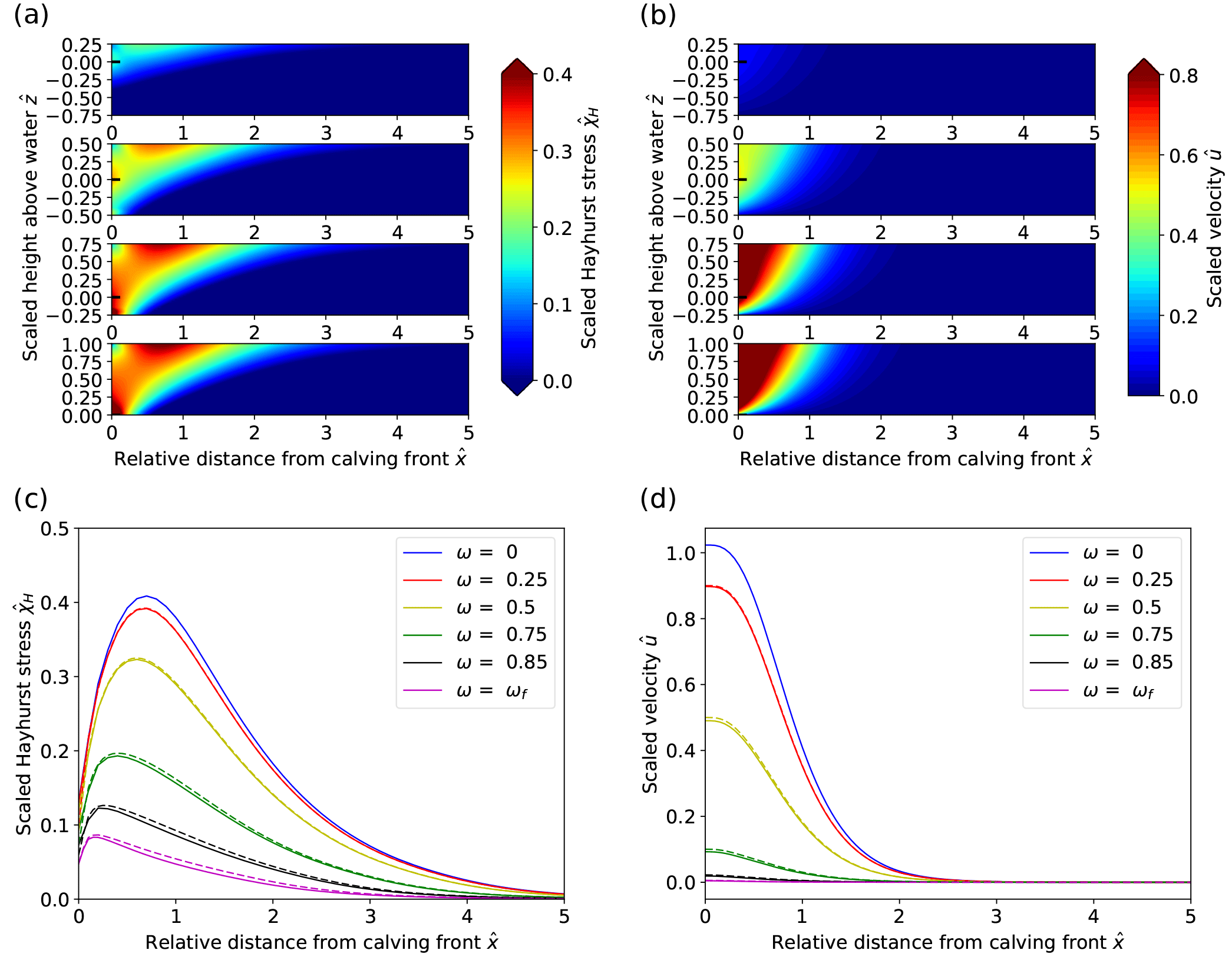
Figure 3Sensitivity experiment results for varying water depth. (a) Scaled Hayhurst stress distribution. (b) Scaled horizontal velocity distributions. (c) Scaled Hayhurst stress along the surface. (d) Scaled horizontal velocity magnitude along the surface. In panels (a, b), the subplots show increasing water depth from the bottom to the top (water level at ). Solid and dashed lines in panels (c, d) correspond to experiments with sea- and freshwater densities, respectively.
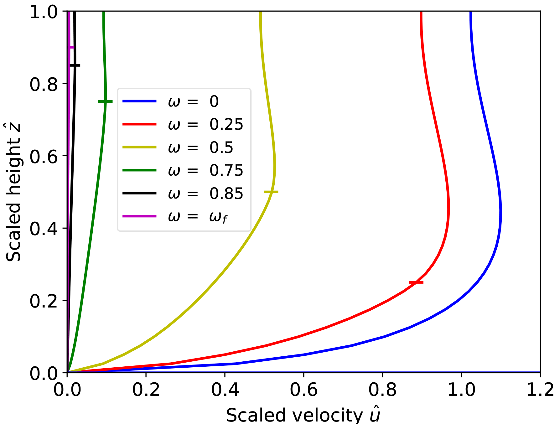
Figure 4Scaled velocities along the vertical face of the calving front (solid lines) for different relative water levels. Horizontal line markers show the relative water level for each curve.
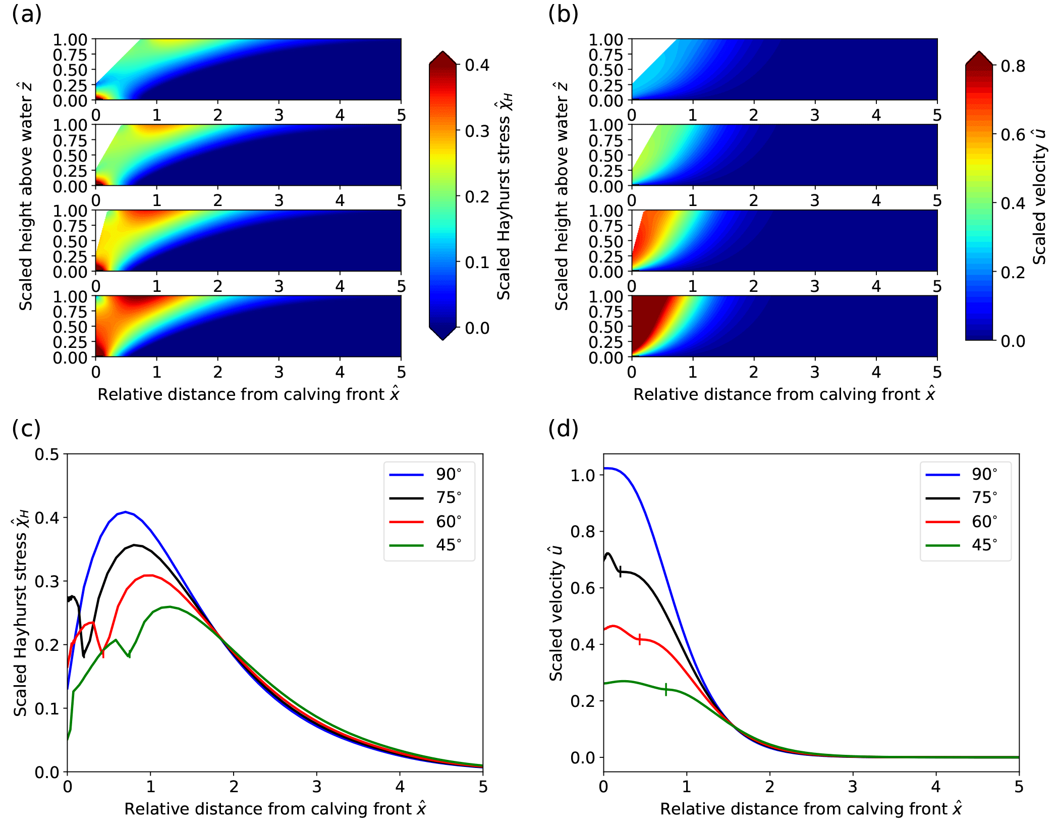
Figure 5Sensitivity experiment results for varying calving front slope. Panels (a–d) are the same as Fig. 3. In panels (a, b), the subplots show decreasing calving front slopes from the bottom to the top. In panel (c), the local minimum of stress close to the calving front is located where the front reaches its maximal height. In panel (d), vertical lines on the curves for inclined fronts mark the distance at which the maximal surface height is reached.
To investigate the full spectrum of possible stress states that lead to the initiation of damage, we investigated linear combinations of five stress invariants: and additionally the third invariant of the stress tensor I3=det(σ) and third invariant of the deviatoric stress tensor . This extended linear combination reads
with weights and μ that fulfill the conditions
We performed a sensitivity analysis based on the five stress invariants of Eq. (14) by systematically varying the weights with 0.1 increments (Eq. 15).
3.1 Sensitivity analyses
All sensitivity experiment results shown in Figs. 3, 5 and 6 exhibit similar velocity and stress patterns. The effects of varying water level, basal slipperiness and calving front slope on the stress field are displayed as Hayhurst stress with parameters chosen according to Pralong and Funk (2005) (Table 1). In general, the modeled velocities and stresses increase towards the calving front, with a local stress maximum at the surface that is located less than one ice thickness upstream of the calving front. This zone of high stress extends diagonally down towards the calving front where it has a second local maximum closely above the water level. For experiments with a relatively low water level, the absolute maxima in stress are found at the bottom of the calving face.
3.1.1 Water level height
The depth of the water at the calving front significantly impacts the stress regime and consequently the ice flow pattern and magnitude near the terminus. The effect of different water depths on the stress field is displayed as Hayhurst stress in Fig. 3a and c.
For a reduction in the relative water level from ω=ωf to ω=0 the maximum Hayhurst stress at the surface increases from 0.08 to 0.42 σref and the location of the stress peak at the surface moves from 0.1 to 0.5 H upstream of the front, whereas the Hayhurst stress at the vertical calving front increases from 0.15 to 0.81 σref. Interestingly, the local maxima at the front are always located near the water level. Further, the position of the global stress maximum for low water levels (below 0.25) is found at the bottom of the calving front instead of the surface (Table 2).
Figures 3b, d and 4 illustrate how velocities close to the calving front increase by more than 1 order of magnitude when the water level is decreased from near flotation (ω=0.85) to shallow water (ω=0.25). Note that for all water depths the velocities are only affected up to approximately 2.5 ice thicknesses upstream from the front.
Extrusion flow, a velocity pattern for which maximum horizontal velocity occurs below the surface (Waddington, 2010), is clearly visible in Fig. 4 in the vicinity of the calving front for the low water level cases. This pattern of extrusion flow near the terminus was also observed by Hanson and Hooke (2000) and Leysinger-Vieli and Gudmundsson (2004).
In summary, increasing relative water depth leads to decreased flow velocities and lower stresses and moves the peak of the Hayhurst stress at the surface closer to the front.
Table 2Maximum scaled Hayhurst stress and velocity for water depth experiments. The s and f letters indicate whether the scaled Hayhurst stress maxima were found at the surface or at the bottom of the calving front, respectively.
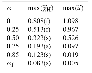
Table 3Maximum Hayhurst stress and velocity for calving front slope experiments.
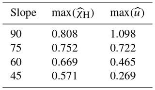
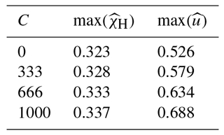
Table 4Maximum Hayhurst stress and velocity for bed slipperiness coefficient experiments.
3.1.2 Calving front slope
Results from the sensitivity experiment on calving front slope displayed in Fig. 5 show large variations in stresses and flow speeds. Maximum Hayhurst stresses are found at the bottom of the calving front for all cases ranging from 0.57 to 0.81 σref for slope angles between 45 and 90∘ (Table 3). A second, local maximum occurs at the surface behind the end of the slope, but the magnitude strongly decreases with decreasing slope. The maximum velocity for a 45∘ slope is ∼4 times smaller than for a vertical calving front (Fig. 5d). Thus, as the calving front gets steeper, the stresses and the velocities increase. Again, the peak in Hayhurst stress at the surface moves further upstream as the calving front is becoming more gentle and a further local stress maximum occurs along the sloped surface. Moreover, the velocities along the surface peak not towards the front corner as in the vertical front case but rather towards the bottom of the sloped surface, which is another sign of extrusion flow.

Figure 7Sensitivity experiments result for an inclined surface (c, f), reverse bed (a, d) and the simple rectangular geometry (b, e). The left and right panels show the scaled Hayhurst stress and velocity distributions, respectively.
3.1.3 Bed slipperiness
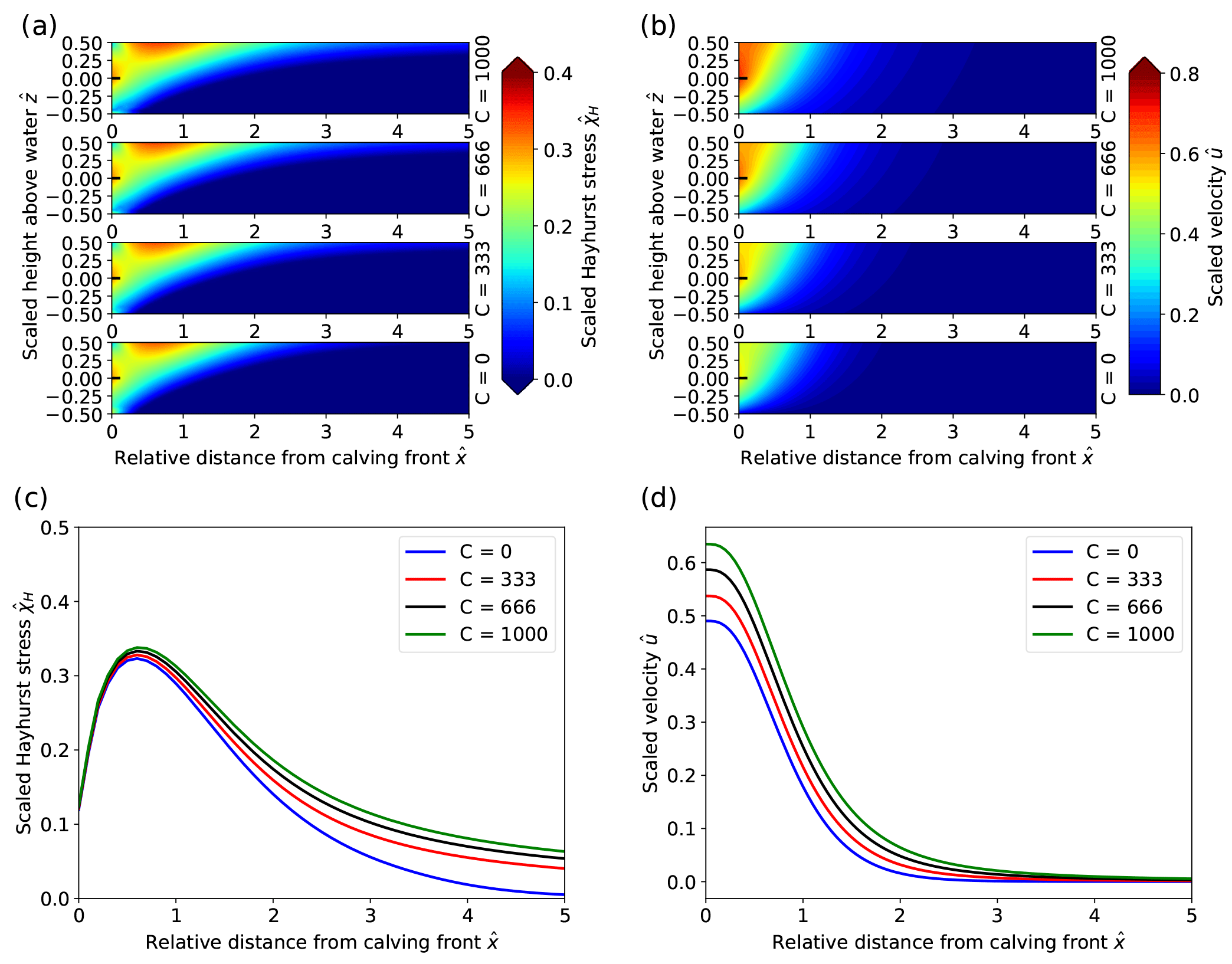
The flow and stress regimes of the idealized glacier are less sensitive to an increase of bed slipperiness coefficient. Figure 6 shows that increased bed slipperiness leads to a slight increase in flow velocity, and the affected zone at the surface extends from three ice thicknesses in horizontal distance from the front to five ice thicknesses. Increasing the bed slipperiness coefficient produces very little effect near the front but causes a substantial increase of the stresses further upstream. The differences in the magnitudes of the Hayhurst stress maximum at the surface are, however, relatively small compared to the variations from other sensitivity experiments. The locations of the stress maxima remain the same for all bed slipperiness sensitivity experiments. Moreover, the spatial distributions of Hayhurst stress and velocity remain qualitatively very similar throughout the domain for the different bed slipperiness coefficients, and differences are mostly apparent at the surface.
3.1.4 Bed and surface slope
In the modeling presented so far we used a glacier geometry with horizontal surface and bed. Consequently the driving stress and hence velocities and stresses far upstream from the calving front are close to zero. In reality glaciers have a sloping surface. Therefore, we repeated some of the above experiments on a simple glacier geometry with a sloped bed and surface, a fixed cliff height and no sliding. Bed and surface slopes were chosen as −5 and 5∘, respectively. Figure 7 illustrates the results: a reclining slope at the surface (i.e., surface height increasing towards the inland) with a flat bed leads to higher stresses and velocities upstream of the calving front as compared to the flat surface. However, the stress maximum and its location in the vicinity of the calving front remains almost identical (Fig. 7b, c). Similar results are obtained for a reverse bed slope with a flat surface (Fig. 7a, b).
To summarize, the stress and velocity fields in the vicinity of the calving front are only slightly altered for sloping bed and surface. It is, however, noteworthy that the reclining surface slope induces higher stresses near the surface, which could potentially induce crevassing and thus advect pre-damaged ice to the calving front.
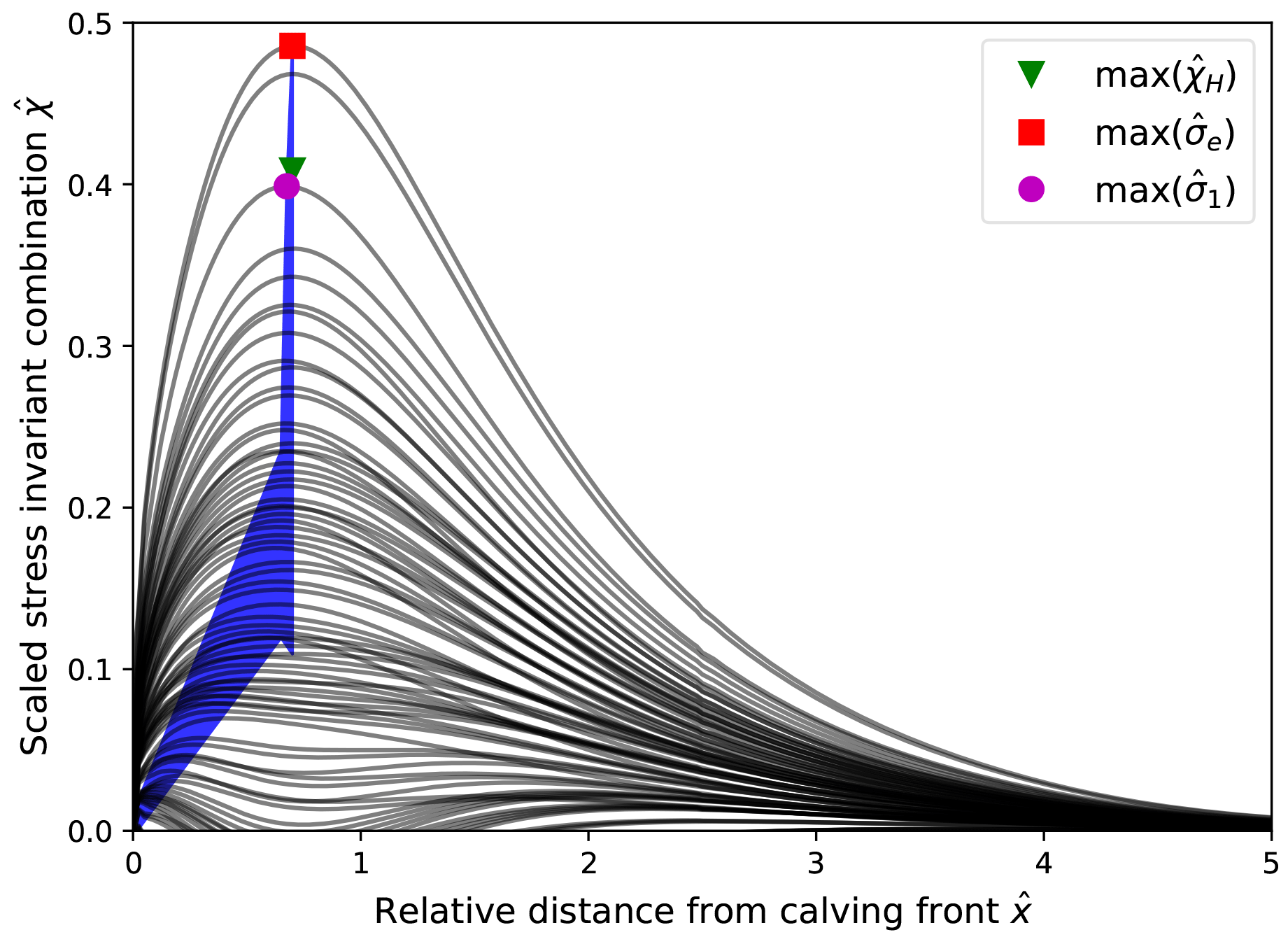
Figure 8Combinations of five stress tensor invariants at the surface of an idealized glacier with a vertical calving front without water pressure and zero basal motion. Each black line represents a linear combination of five stress invariants. The blue envelope contains the maxima of all stress invariant combinations. The green triangle, red square and purple circle represent the maximum of the scaled Hayhurst stress , von Mises stress and maximum principal stress , respectively.
3.2 Stress invariant combinations
The Hayhurst stress, typically used as the driving force for damage evolution (Duddu and Waisman, 2012, 2013; Duddu et al., 2013; Mobasher et al., 2016; Pralong and Funk, 2005; Pralong et al., 2003), is not the only possible combination of objective stress measures. Here we attempt a systematic analysis of the possible stress invariant combinations (Eq. 14) and the corresponding locations of the stress maxima along the glacier surface. We illustrate this analysis at the example of the block geometry without any water pressure (ω=0) in Fig. 8, where all possible linear combinations of five stress invariants along the surface are displayed. While the stress combinations show a wide variety of curves, the maximum achievable stress states are dominated by the von Mises stress σe and the maximum principal stress σ1, both of which contribute to the Hayhurst stress. Hence, these two stress invariants are likely the driving factors for material failure in the vicinity of the calving front. An important aspect illustrated in Fig. 8 is the horizontal position of the stress maximum, which is limited to xmax≃0.7 Href. This analysis thus suggests that a zone with maximum crevasse opening cannot be located in greater distance from the calving front than xmax for an idealized glacier without pre-damaged ice.
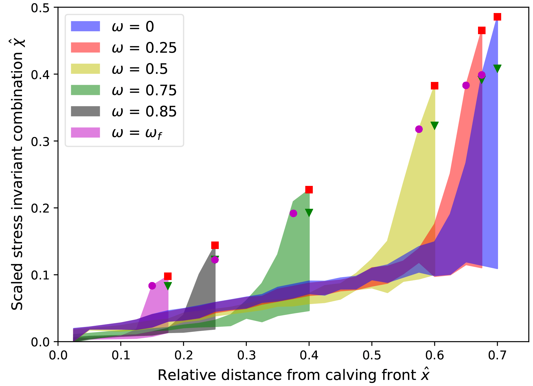
Figure 9Envelopes of stress invariant combinations at the surface of the idealized glacier with zero basal motion for varying relative water level ω. The green triangle, red square and purple circle represent the maximum of the scaled Hayhurst stress, von Mises stress and maximum principal stress, respectively, for each water depth.
The magnitudes and positions of the maximum stress invariant combinations for different relative water levels ω are shown in Fig. 9 (blue area corresponds to Fig. 8). The maximum stress for dry conditions (ω=0) is located ∼0.7 Href from the calving front with a maximum von Mises stress of ∼ 0.45 σref, whereas a water level close to flotation (ω=0.85) leads to a stress maximum of ∼0.15 σref at ∼0.25Href from the calving front. Figure 9 clearly illustrates that water pressure at the calving front exerts a stabilizing effect on the calving front by both lowering the stresses and decreasing the distance from the calving front at which the stress maximum is located, as argued earlier by Bassis and Walker (2012).
The Hayhurst, maximum principal and von Mises stress distributions are shown in Figs. 3a, B1a and B1b, respectively.
The similarity of stress distribution curves along the glacier surface for varying relative water levels (Fig. 3c) allows for an explicit parametrization of the stresses. With some simple assumptions on a damage evolution law, a calving rate parametrization can be derived that is expressed as a function of total ice thickness and relative water level. Specifically, we assume that surface crevasses open under the extensional stress σ1. The Hayhurst stress would be a similarly suited stress measure for the extensional stress state under small compressive load at the glacier surface. The above stress state analysis showed that the three stress intensity measures σ1, σe and χH along the glacier surface are very similar, as demonstrated in Fig. 9.
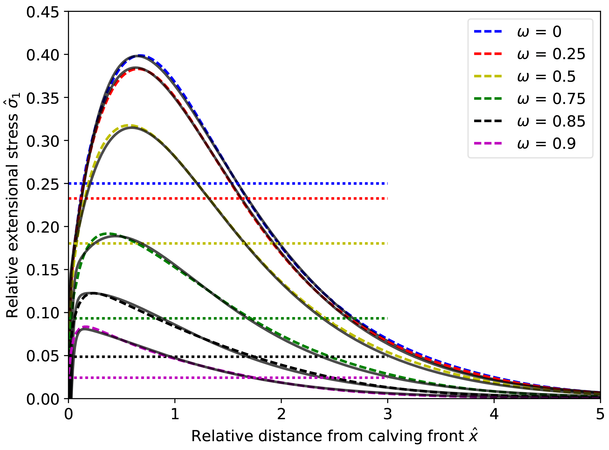
Figure 10Modeled (dashed lines) and corresponding parametrized (solid lines) maximum extensive stresses at the surface for different water depths. The dotted lines show the horizontal deviatoric stresses at the calving front for all water depths based on Eq. (1).
4.1 Stress parametrization
The distribution along the glacier surface of scaled maximum principal stress is shown for different relative water levels in Fig. 10 (this is approximately the tensile stress along the surface, whereas Fig. 3c shows Hayhurst stress). The similarity in shape of these stress curves allows for an approximate representation by a function that depends on the relative water level ω alone:
where is a stretched and shifted version of the scaled (by ice thickness) horizontal coordinate . This stretching function is somewhat cumbersome and is given in Appendix A. The extensional stress reaches the maximum at (setting the derivative of Eq. 16 to 0) with magnitude and can be approximated by
It is interesting to note that the maximum extensional stress at the surface has a similar form as the mean deviatoric stress in Eq. (1) but is ∼60 % higher. The scaled horizontal position of the stress maximum can be approximated by
4.2 Analytical calving relation
Using the parametrizations of magnitude and position of the maximum extensional stress at the surface (Eqs. 17a and 18) the calving rate can be estimated under simple assumptions on crevasse formation.
One major assumption is that a large crevasse forms at the location of the maximum tensile surface stress where the ice is weakened until failure. Such crevassing seems realistic as both observations and model results show the formation of huge crevasses. When failure of the surface ice is complete, we assume that all ice in front of the crevasse is removed and a new calving front forms at the location of the crevasse. Here, we do not consider explicitly which processes are responsible for downward propagation of the crevasse. Several processes could be considered, such as bottom crevassing, hydro-fracturing by ponding water in surface crevasses, rapid elastic crevasse propagation (Krug et al., 2014), ice break-off in multiple steps (e.g., a surface slump, followed by subaqueous buoyant calving) or continued material fatigue due to tidal forcing. The proposed calving relation relies on the major assumption that processes responsible for ice break-off act on faster timescales than the formation of the surface crevasse and, therefore, that the calving process is uniquely determined by the time to failure at the surface stress maximum. Thus, the average calving rate can be calculated as the distance of the stress maximum divided by the time to failure Tf. In dimensional coordinates this is
Assuming further that crevasse formation can be described by isotropic damage formation with damage variable D, the stress in the damaged material is (Pralong, 2006; Pralong et al., 2003). The isotropic damage evolution relationship employed here is
where B is the rate factor for damage evolution, r and k are constants, σ0 is the stress in the work zone and σth a stress threshold for damage creation. Integrating this relation over time, the time to failure, i.e., the time required for damage to evolve from an initial value D0 to a critical value Dc, reads
We further assume that the stress in the work zone is the maximum tensile stress . Inserting the parametrizations for maximum tensile stress and stress maximum position (Eqs. 17c and 18) in the above relation yields
The term in square brackets is constant, and after renaming it the effective damage rate the expression reads
with parameter values and σth=0.17 MPa, which were determined from a calibration with data discussed below in Sect. 5.3. The parameter value r=0.43 is chosen according to Pralong and Funk (2005).
5.1 Sensitivity analyses
The stress intensity and therefore ice deformation rates are decreasing as the relative water level increases due to the pressure exerted by the water at the calving front. This feature is already captured by the depth-integrated extensional stress at the front (Eq. 1) and, in more detail, in the parametrized maximum extensional stress (Eq. 17a), illustrated in Fig. 10. In both cases the square dependence of the horizontal stress on relative water level controls fracture or damaging processes, the magnitude and rate of which depend linearly on the stress intensity.
In addition, the detailed modeling shows that the stress peak at the glacier surface moves upstream for lowering relative water level (Figs. 3 and 10), implying that crevasses are likely to open in greater distance from the calving front and leading to detachment of larger masses during calving.
A higher relative water level results in a more stable calving front (Bassis and Walker, 2012), which seems to be in contrast with the often-used relations which predict that calving rates increase with water depth (Brown et al., 1982; Hanson and Hooke, 2000; Meier and Post, 1987). In nature, however, glaciers terminating in deeper waters are also thicker and calve at higher rates as they experience higher absolute (unscaled) stresses. Furthermore, submarine frontal melting is likely to lead to higher calving rates by over-steepening of the front (O'Leary and Christoffersen, 2013), although the melt undercutting effect on calving rates seems to be limited (Cook et al., 2014; Krug et al., 2015).
Using freshwater instead of seawater at the calving front yields slightly higher stresses and velocities (Fig. 3c, d). This difference can be explained by the reduced back pressure applied by freshwater on the calving front, which results from a lower water density.
The model results demonstrate that reclining calving fronts lead to lower velocities and stresses and thereby implicitly confirm that inclined calving fronts should reach larger stable heights than vertical cliffs, as observed for example at Eqip Sermia (200 m high at 45∘). This sensitivity analysis on front slope may, together with observational data on non-vertical calving fronts, provide constraints on parameters of ice resistance to failure. Further, the presence of extrusion flow along the reclining calving face of an idealized glacier was demonstrated. Such a velocity pattern has been observed and measured on an inclined slope at the northern front of Eqip Sermia (Lüthi et al., 2016) but is rarely discussed in modeling studies (Hanson and Hooke, 2000; Leysinger-Vieli and Gudmundsson, 2004).
Basal sliding leads to increased stresses at the surface throughout the computational domain. Thus, basal sliding may cause an onset of ice damaging and crevasse opening in a greater distance from the calving front (Fig. 6c). The velocity patterns in Fig. 6b show that the influence of bed slipperiness is only apparent in the proximity of the calving front, even for high sliding coefficients. Moreover, stress distributions are almost identical for all bed slipperiness experiments, which implies that basal sliding has a negligible effect on the stability of the calving front. Basal sliding adds a constant velocity at the bottom of the domain rather than affecting the velocity gradients. This result does not include any spatial variation in bed slipperiness, which would likely be caused by including a water-pressure-dependent sliding relation. Effective pressure (the difference between ice normal stress at the bottom and water pressure) typically decreases towards the calving front for real glaciers with sloping surface and may cause additional sliding towards the front, an effect that is not considered in this modeling effort.
For a sloping glacier surface the location and magnitude of the stress maximum in the vicinity of the calving front remain almost identical, as shown in Fig. 7. Similar results are obtained for a reverse bed slope with a flat surface, with a smaller influence on stresses and velocities than for the reclining surface. However, the effect on stresses and velocities upstream of the calving front is not visible for the reverse bed slope with a flat surface. This indicates that, for a glacier with a reclining surface slope, ice can potentially start damaging and forming crevasses at the surface far upstream from the calving front.
5.2 Calving relation
The proposed calving rate parametrization (Eq. 22) is simple and only requires two geometrical quantities: frontal ice thickness H and water depth Hw. The assumptions about the failure process are lumped into three parameters – , σth and r – which can be determined by data calibration (Sect. 5.3). The parametrization exhibits many similarities with established calving relations but is formulated in terms of two quantities that are calculated by any ice flow model. It therefore is a drop-in replacement for other calving relations used in glacier models of different complexity.
The calving rate parametrization (Eq. 22) has some interesting properties, which are illustrated in Figs. 11 and 12. Holding constant the relative water depth, the absolute water depth or the ice thickness results in different calving laws:
-
for constant relative water level ω the calving rate grows roughly like (black and gray lines in Fig. 11);
-
for constant absolute water depth Hw=ωH a fit shows that roughly (red and orange lines in Fig. 11);
-
for constant ice thickness the calving rate decreases with increasing relative water level (Fig. 12) roughly like
The predicted calving rate for a given water depth depends on the thickness of the glacier, which is the result of the mass fluxes in the terminus area. Thus, calving rates depend on the surface evolution and hence the upstream dynamics of the glacier. The semi-empirical calving rate parametrization is therefore, in the sense of inclusion of upstream dynamics, similar to the position based calving models (Benn et al., 2007a, 2017; Nick et al., 2010; Todd and Christoffersen, 2014). The formulation as a calving rate also makes this parametrization relatively easy to use in larger-scale fixed grid models.
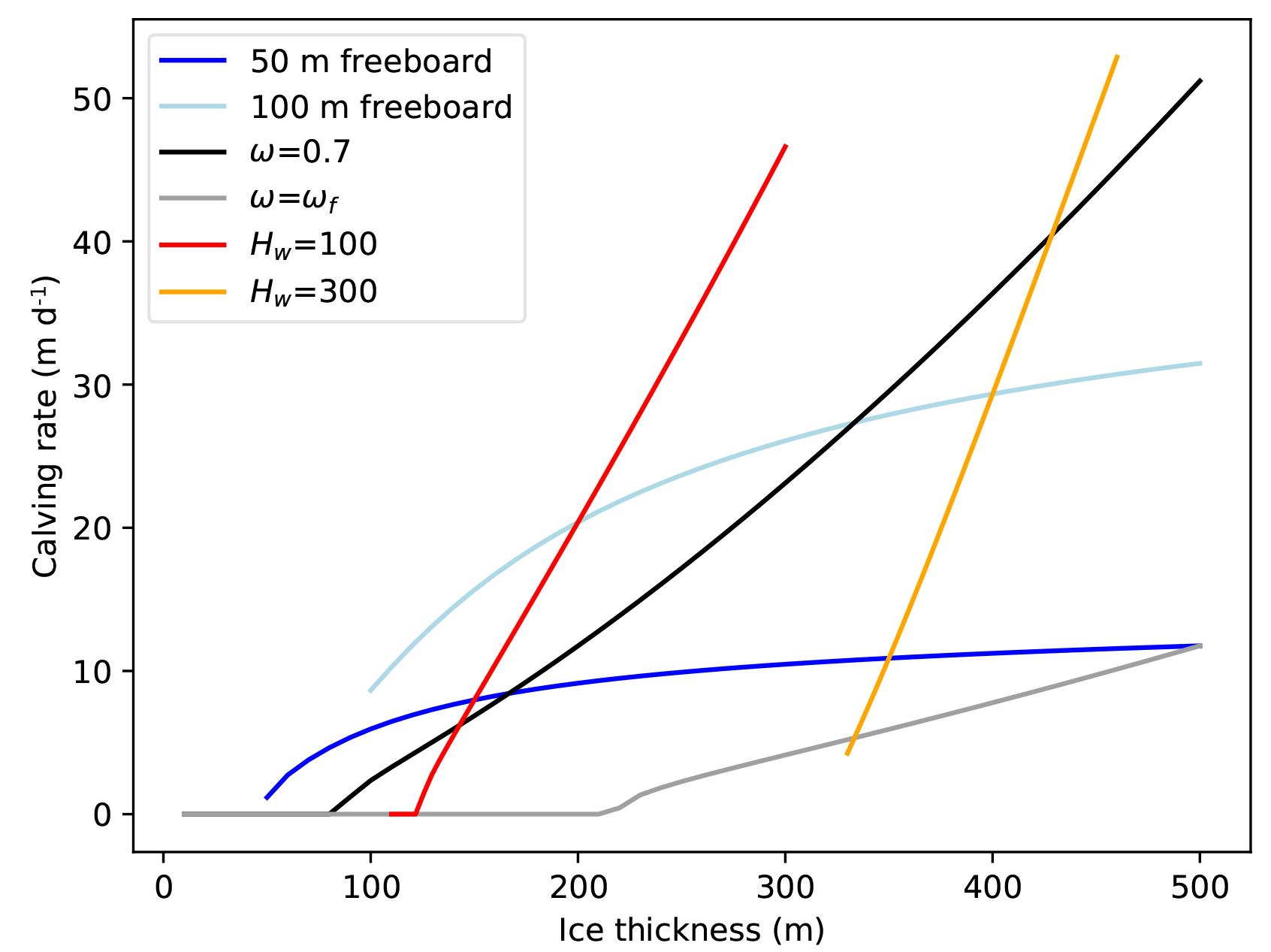
Figure 11Calving rates predicted by the parametrization in relation to ice thickness. Calving rates increase with increasing total ice thickness for a given water depth Hw=ωH (red and orange lines), relative water level ω (black and gray lines) or freeboard H−Hw (blue lines). Note that the gray line refers to a front at flotation.
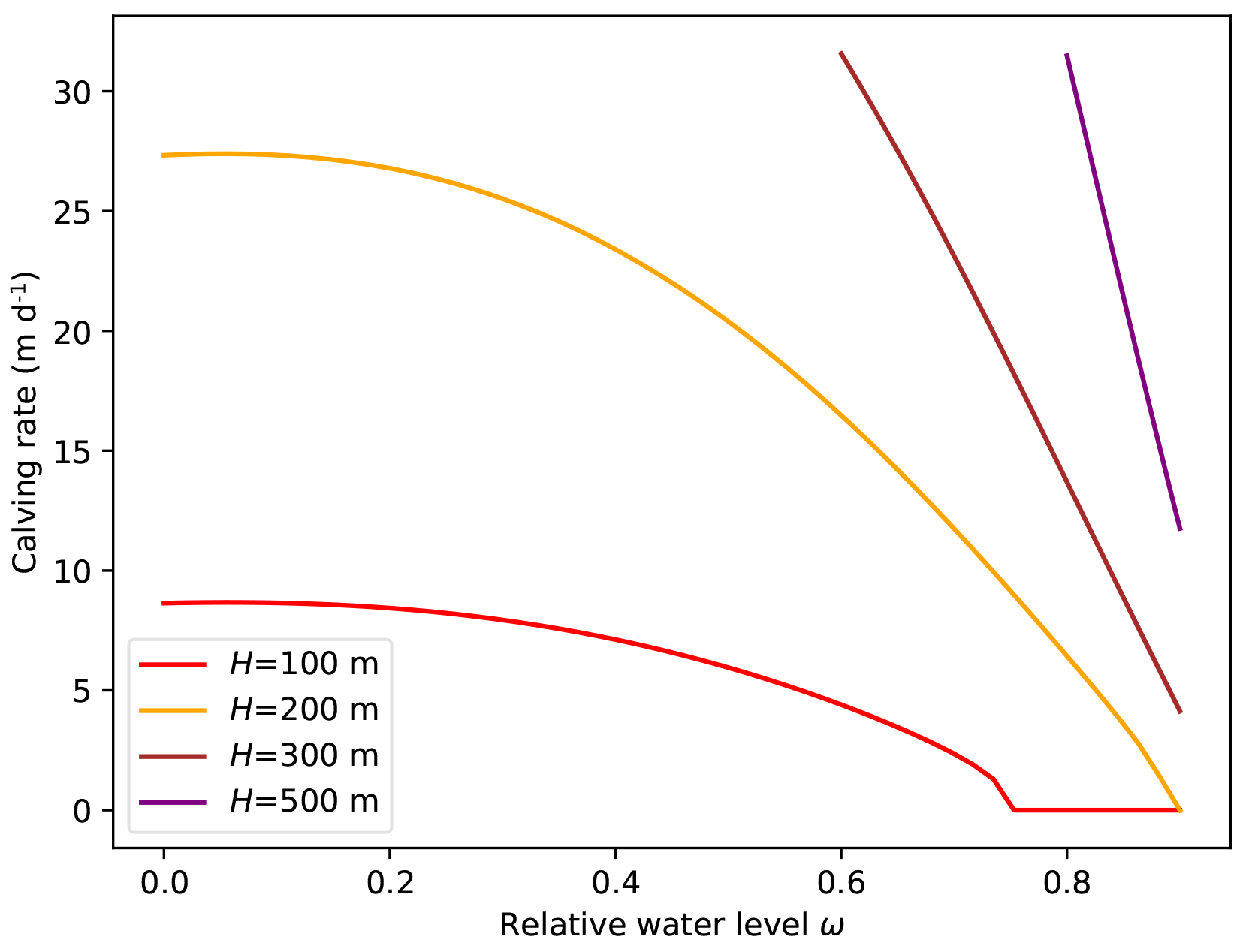
Figure 12Calving rates predicted by the parametrization as a function of relative water level. Calving rate decreases under increase of the relative water level ω for constant total ice thickness H.

Figure 13Calving rates (m d−1) predicted by the parametrization are shown as contours in dependence of H and ω. The hatched region indicates the states excluded by the maximum calving front criterion (Bassis and Walker, 2012). The gray area indicates states where the stress threshold σth precludes calving. Blue dots with numbers indicate calving rates determined from measurements, shown in Table 5.
5.3 Calibration of the parametrization
The calving rate parametrization (Eq. 22) contains three empirical parameters: and σth=0.17 MPa, which were obtained by calibration with data, and r=0.43, which is taken from Pralong and Funk (2005). Calving rates thus obtained are not very sensitive to the exact choice of parameter values, which are within the range of previous studies (Duddu and Waisman, 2012; Lliboutry, 2002; Vaughan, 1993).
Sugiyama et al. (2015)Pfeffer (2007)Pfeffer (2007)Pfeffer (2007)Pfeffer (2007)Pfeffer (2007)Lüthi et al. (2016); Rignot et al. (2015)Murray et al. (2015); Voytenko et al. (2015)Carr et al. (2015)Carr et al. (2015)Lüthi et al. (2009)Carbonnell and Bauer (1968)Carbonnell and Bauer (1968)Pralong (2006)Carbonnell and Bauer (1968)Carbonnell and Bauer (1968)Rignot et al. (2015); Ryan et al. (2015)Trüssel et al. (2015)Table 5Values of calving front height, water depth and calving rate for different glaciers.
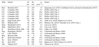
To calibrate these parameter choices, data on calving rate, ice thickness and water depth for a wide variety of tidewater glaciers in the Arctic were collected. The data set covers the full range of water levels (relative and absolute), velocities and ice thicknesses that are found in Arctic tidewater glaciers. Unfortunately, many studies report only width-averaged data on calving front geometry and calving rate, which are not suitable for our proposed relation which relies on local stresses on a flowline. Only a limited set of point data on calving front geometries are available from the published literature from which total ice cliff thickness, water depth and calving rate can be obtained. For the calibration, we used the values shown in Table 5 from diverse data sources.
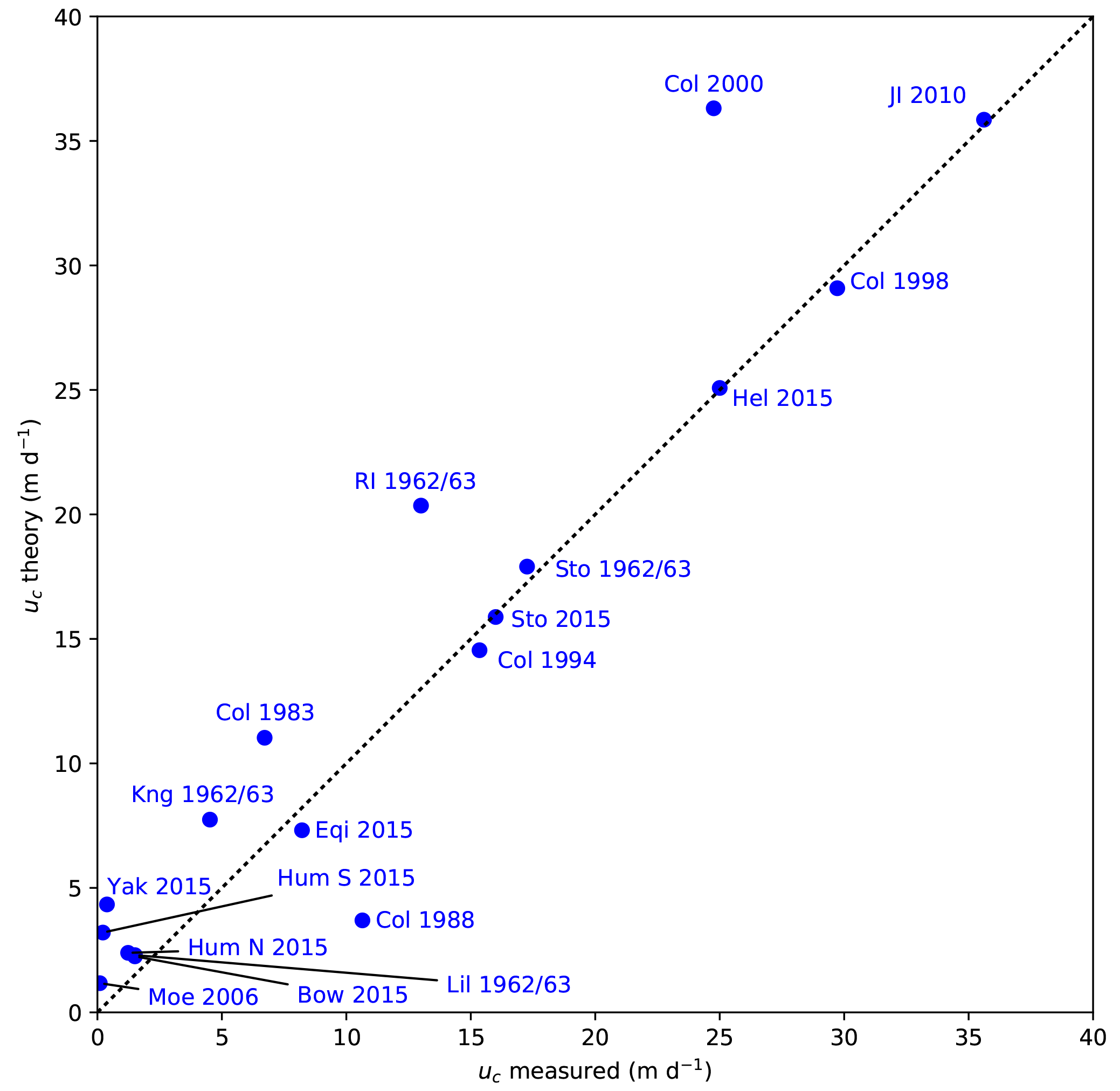
Contours of calving rates calculated with Eq. (22) are shown in Fig. 13 together with the maximum theoretical calving front height predicted by Bassis and Walker (2012). Figure 14 plots the same calving rate data against results from the parametrization. While a sizable spread of the data is visible, especially for low calving rates, the general agreement shows that the parametrization is well suited to estimate calving rates for this set of tidewater glaciers in the Arctic.
Note that the derivation of the parametrization is independent of the specific geometry or location of a tidewater glacier and thus the calibration is expected to be “global” and valid for any tidewater glacier.
This study improves our knowledge on the influence of geometry and water depth on the stress and flow regimes in the vicinity of the calving front and proposes a novel calving rate parametrization.
The magnitude of the stresses and flow speeds near a grounded vertical calving front are dominantly dependent on water depth and increase with decreasing water depth. Thus, the presence of water at the calving front has a strong stabilizing effect. Importantly, the extensional stress at the surface can be parametrized as a function of relative water level only. Further, we find that grounded tidewater glaciers with reclining calving faces have the potential to reach larger maximum stable heights than those with vertical calving fronts. Spatially uniform variations in basal sliding likely have a weaker effect than water depth and calving front slope on the stability, as the magnitude and location of the stress maximum show a small sensitivity to variations in bed slipperiness.
A simple calving rate parametrization was derived that was calibrated with calving rate data of a set of tidewater glaciers in the Arctic. This approach can be used to compute calving rates for grounded tidewater glaciers with relatively simple geometries when front thickness and water depth are known. The application of this parametrization in flow models of different complexity should be straightforward.
The present study lays the foundation for future, more detailed, studies of the calving process on more realistic geometries. Detailed analyses including time evolution, further processes such as frontal melt and water-filled crevasses, and data validation will be necessary for the implementation of improved calving parametrizations.
The libMesh library is a C++ framework for the numerical simulation of partial differential equations on serial and parallel platforms available at http://libmesh.github.io/ (Kirk et al., 2006). Data from this study can be made available from the authors upon request.
The distribution of longitudinal tensile stress at the surface can be fitted using stretched and scaled coordinates depending on relative water level ω:
The stress fit includes a taper towards the calving front which was chosen as an exponential. The full approximation to the stress curve is given by
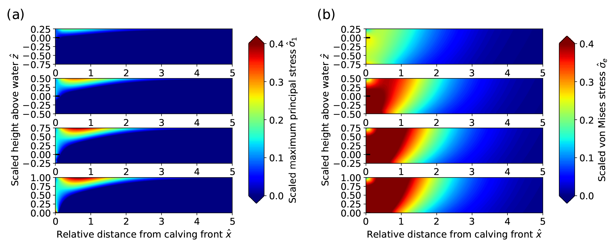
Figure B1 Stress distributions for varying water depth. (a) Scaled maximum principal stress distribution. (b) Scaled von Mises stress distribution.
The authors declare that they have no conflict of interest.
The authors wish to thank Jaime Otero and Jeremy Bassis for their reviews
and Douglas Benn, Joe Todd and Olivier Gagliardini for their comments that
helped considerably to improve this paper. This work was funded by the
Swiss National Science Foundation Grant 200021_156098.
Edited by: Olivier Gagliardini
Reviewed by: Jeremy Bassis and Jaime Otero
Amundson, J., Fahnestock, M., Truffer, M., Brown, J., Lüthi, M., and Motyka, R.: Ice mélange dynamics and implications for terminus stability, Jakobshavn Isbræ, Greenland, J. Geophys. Res., 115, F01005, https://doi.org/10.1029/2009JF001405, 2010. a
Balay, S., Buschelman, K., Eijkhout, V., Gropp, W. D., Kaushik, D., Knepley, M. G., McInnes, L. C., Smith, B. F., and Zhang, H.: PETSc Users Manual, Tech. Rep. ANL-95/11 – Revision 3.0.0, Argonne National Laboratory, available at: http://www.mcs.anl.gov/petsc (last access: 2 March 2017), 2008. a
Bassis, J. N. and Walker, C. C.: Upper and lower limits on the stability of calving glaciers from the yield strength envelope of ice, P. Roy. Soc. Lond. A Mat., 468, 913–931, https://doi.org/10.1098/rspa.2011.0422, 2012. a, b, c, d, e, f, g
Benn, D. I., Hulton, N. R., and Mottram, R. H.: `Calving laws', `sliding laws' and the stability of tidewater glaciers, Ann. Glaciol., 46, 123–130, 2007a. a, b
Benn, D. I., Warren, C. R., and Mottram, R. H.: Calving processes and the dynamics of calving glaciers, Earth-Sci. Rev., 82, 143–179, https://doi.org/10.1016/j.earscirev.2007.02.002, 2007b. a, b
Benn, D. I., Aström, J., Todd, J., Nick, F. M., Hulton, N. R., and Luckman, A.: Melt-undercutting and buoyancy-driven calving from tidewater glaciers: new insights from discrete element and continuum model simulations, J. Glaciol., 63, 691–702, 2017. a, b, c
Brown, C. S., Meier, M. F., and Post, A.: Calving speed of Alaska tidewater glaciers, with application to Columbia glacier, Tech. rep., US Geological survey professional paper 1258-C,, available at: https://pubs.er.usgs.gov/publication/pp1258C (last access: 22 January 2017), 1982. a, b
Carbonnell, M. and Bauer, A.: Exploitation des couvertures photographiques aériennes répétées du front des glaciers vêlants dans Disko Bugt et Umanak Fjord, Juin-Juillet 1964, Tech. Rep. 3, Expédition glaciologique internationale au Groenland (EGIG), tirage à part des Meddelelser om Grønland, Bd. 173, Nr. 5, København, Lunos, 1968. a, b, c, d
Carr, J., Stokes, C., and Vieli, A.: Recent progress in understanding marine-terminating Arctic outlet glacier response to climatic and oceanic forcing: twenty years of rapid change, Prog. Phys. Geog., 37, 436–467, https://doi.org/10.1177/0309133313483163, 2013. a
Carr, J., Vieli, A., Stokes, C., Jamieson, S., Palmer, S., Christoffersen, P., Dowdeswell, J., Nick, F., Blankenship, D., and Young, D.: Basal topographic controls on rapid retreat of Humboldt Glacier, nothern Greenland, J. Glaciol., 61, 137–150, https://doi.org/10.3189/2015JoG14J128, 2015. a, b
Cook, S., Rutt, I. C., Murray, T., Luckman, A., Zwinger, T., Selmes, N., Goldsack, A., and James, T. D.: Modelling environmental influences on calving at Helheim Glacier in eastern Greenland, The Cryosphere, 8, 827–841, https://doi.org/10.5194/tc-8-827-2014, 2014. a, b, c
Cowton, T., Sole, A., Nienow, P., Slater, D., Wilton, D., and Hanna, E.: Controls on the transport of oceanic heat to Kangerdlugssuaq Glacier, East Greenland, J. Glaciol., 62, 1167–118, https://doi.org/10.1017/jog.2016.117, 2016. a
Cuffey, K. and Paterson, W.: The Physics of Glaciers, Elsevier, Burlington, MA, USA, iSBN 978-0-12-369461-4, 2010. a, b
Duddu, R. and Waisman, H.: A temperature dependent creep damage model for polycrystalline ice, Mech. Mater., 46, 23–41, 2012. a, b, c
Duddu, R. and Waisman, H.: A non local continuum damage mechanics approach to simulation of creep fracture in ice sheets, Comput. Mech., 51, 961–974, 2013. a, b
Duddu, R., Bassis, J. N., and Waisman, H.: A numerical investigation of surface crevasse propagation in glaciers using nonlocal continuum damage mechanics, Geophys. Res. Lett., 40, 3064–3068, 2013. a, b
Greve, R. and Blatter, H.: Dynamics of Ice Sheets and Glaciers, Springer-Verlag, Heidelberg, iSBN 978-3-642-03414-5, 2009. a
Gudmundsson, G. H. and Raymond, M.: On the limit to resolution and information on basal properties obtainable from surface data on ice streams, The Cryosphere, 2, 167–178, https://doi.org/10.5194/tc-2-167-2008, 2008. a
Hanson, B. and Hooke, R. L.: Glacier calving: a numerical model of forces in the calving-speed/water-depth relation, J. Glaciol., 46, 188–196, 2000. a, b, c, d, e
Hayhurst, D. R.: Creep rupture under multi-axial states of stress, J. Mech. Phys. Solids, 20, 381–390, 1972. a
Howat, I. M., Box, J. E., Ahn, Y., Herrington, A., and McFadden, E. M.: Seasonal variability in the dynamics of marine terminating outlet glaciers in Greenland, J. Glaciol., 56, 601–613, https://doi.org/10.3189/002214310793146232, 2010. a
Joughin, I., Das, S. B., King, M. A., Smith, B. E., Howat, I. M., and Moon, T.: Seasonal speedup along the western flank of the Greenland Ice Sheet, Science, 320, 781–783, https://doi.org/10.1126/science.1153288, 2008. a
Kirk, B., Peterson, J. W., Stogner, R. H., and Carey, G. F.: libMesh:
a C++ Library for Parallel
Adaptive Mesh Refinement/Coarsening Simulations, Eng. Comput., 22, 237–254, https://doi.org/10.1007/s00366-006-0049-3, 2006. a
Krug, J., Weiss, J., Gagliardini, O., and Durand, G.: Combining damage and fracture mechanics to model calving, The Cryosphere, 8, 2101–2117, https://doi.org/10.5194/tc-8-2101-2014, 2014. a, b
Krug, J., Durand, G., Gagliardini, O., and Weiss, J.: Modelling the impact of submarine frontal melting and ice mélange on glacier dynamics, The Cryosphere, 9, 989–1003, https://doi.org/10.5194/tc-9-989-2015, 2015. a, b
Lea, J. M., Mair, D. W. F., Nick, F. M., Rea, B. R., van As, D., Morlighem, M., Nienow, P. W., and Weidick, A.: Fluctuations of a Greenlandic tidewater glacier driven by changes in atmospheric forcing: observations and modelling of Kangiata Nunaata Sermia, 1859–present, The Cryosphere, 8, 2031–2045, https://doi.org/10.5194/tc-8-2031-2014, 2014. a
Leysinger-Vieli, G. J.-M. C. and Gudmundsson, G. H.: On estimating length fluctuations of glaciers caused by changes in climatic forcing, J. Geophys. Res., 109, F01007, https://doi.org/10.1029/2003JF000027, 2004. a, b
Lliboutry, L.: Velocities, strain rates, stresses, crevassing and faulting on Glacier de Saint-Sorlin, French Alps, 1957–1976, J. Glaciol., 48, 125–141, 2002. a
Luckman, A., Benn, D. I., Cottier, F., Bevan, S., Nilsen, F., and Inall, M.: Calving rates at tidewater glaciers vary strongly with ocean temperature, Nat. Commun., 6, 8566, https://doi.org/10.1038/ncomms9566, 2015. a
Lüthi, M. P. and Vieli, A.: Multi-method observation and analysis of a tsunami caused by glacier calving, The Cryosphere, 10, 995–1002, https://doi.org/10.5194/tc-10-995-2016, 2016. a
Lüthi, M. P., Fahnestock, M., and Truffer, M.: Calving icebergs indicate a thick layer of temperate ice at the base of Jakobshavn Isbræ, Greenland, J. Glaciol., 55, 563–566, https://doi.org/10.3189/002214309788816650, 2009. a
Lüthi, M. P., Vieli, A., Moreau, L., Joughin, I., Reisser, M., Small, D., and Stober, M.: A century of geometry and velocity evolution at Eqip Sermia, West Greenland, J. Glaciol., 1–15, https://doi.org/10.1017/jog.2016.38, 2016. a, b, c
Meier, M. F. and Post, A.: Fast tidewater glaciers, J. Geophys. Res., 92, 9051–9058, 1987. a
Mobasher, M., Duddu, R., Bassis, J. N., and Waisman, H.: Modeling hydraulic fracture of glaciers using continuum damage mechanics, J. Glaciol., 62, 794–804, https://doi.org/10.1017/jog.2016.68, 2016. a, b
Motyka, R. J., Dryer, W. P., Amundson, J., Truffer, M., and Fahnestock, M.: Rapid submarine melting driven by subglacial discharge, LeConte Glacier, Alaska, Geophys. Res. Lett., 40, 1–6, https://doi.org/10.1002/grl.51011, 2013. a
Murray, T., Selmes, N., James, T., Edwards, S., Martin, I., O'Farwell, T., Aspey, R., Rutt, I., Nettles, M., and Baugé, T.: Dynamics of glacier calving at the ungrounded margin of Helheim Glacier, southeast Greenland, J. Geophys. Res., 120, 964–982, https://doi.org/10.1002/2015JF003531, 2015. a
Nick, F., Van der Veen, C., Vieli, A., and Benn, D.: A physically based calving model applied to marine outlet glaciers and implications for the glacier dynamics, J. Glaciol., 56, 781–794, 2010. a, b
Nick, F., Vieli, A., Vieli, A., Andersen, M. L., Joughin, I., Payne, A., Edwards, T., Pattyn, F., and van de Wal, R.: Future sea-level rise from Greenland's main outlet glaciers in a warming climate, Nature, 479, 235–238, https://doi.org/10.1038/nature12068, 2013. a, b
Nick, F. M., Vieli, A., Howat, I. M., and Joughin, I.: Large-scale changes in Greenland outlet glacier dynamics triggered at the terminus, Nat. Geosci., 2, 110–114, https://doi.org/10.1038/ngeo394, 2009. a
Nye, J. F.: The distribution of stress and velocity in glaciers and ice-sheets, P. Roy. Soc. Lond. A Mat., 239, 113–133, 1957. a, b
O'Leary, M. and Christoffersen, P.: Calving on tidewater glaciers amplified by submarine frontal melting, The Cryosphere, 7, 119–128, https://doi.org/10.5194/tc-7-119-2013, 2013. a
Otero, J., Navarro, F., Martin, C., Cuadrado, M., and Corcuera, M.: A three-dimentional calving model: numerical experiments on Johnsons Glacier, Livingston Island, Antarctica, J. Glaciol., 56, 200–214, https://doi.org/10.3189/002214310791968539, 2010. a
Otero, J., Navarro, F., Lapazaran, J. J., Welty, E., Puczko, D., and Finkelnbrug, R.: Modeling the controls on the front position of a tidewater glacier in Svalbard, Front. Earth Sci., 5, 200–214, 2017. a
Petlicki, M., Cieply, M., Jania, J. A., Prominska, A., and Kinnard, C.: Calving of a tidewater glacier driven by melting at the waterline, J. Glaciol., 61, 851–863, https://doi.org/10.3189/2015JoG15J062, 2015. a
Pfeffer, T.: A simple mechanism for irreversible tidewater glacier retreat, J. Geophys. Res., 112, F03S25, https://doi.org/10.1029/2006JF000590, 2007. a, b, c, d, e
Post, A., O'Neel, S., Motyka, R., and Streveler, G.: A complex relationship between calving glaciers and climate, EOS T. Am. Geophys. Un., 92, 305–306, https://doi.org/10.1029/2011EO370001, 2011. a
Pralong, A.: Ductile Crevassing, in: Glacier Science and Environmental Change, edited by: Knight, P. G., Blackwell Publishing, Oxford, 62 pp., 2006. a, b
Pralong, A. and Funk, M.: Dynamic damage model of crevasse opening and application to glacier calving, J. Geophys. Res., 110, B01309, https://doi.org/10.1029/2004JB003104, 2005. a, b, c, d, e
Pralong, A., Funk, M., and Lüthi, M. P.: A description of crevasse formation using continuum damage mechanics, Ann. Glaciol., 37, 77–82, 2003. a, b, c
Rignot, E., Fenty, I., Xu, Y., Cai, C., and Kemp, C.: Undercutting of marine-terminating glaciers in West Greenland, Geophys. Res. Lett., 42, 5909–5917, https://doi.org/10.1002/2015GL064236, 2015. a, b
Ryan, J. C., Hubbard, A. L., Box, J. E., Todd, J., Christoffersen, P., Carr, J. R., Holt, T. O., and Snooke, N.: UAV photogrammetry and structure from motion to assess calving dynamics at Store Glacier, a large outlet draining the Greenland ice sheet, The Cryosphere, 9, 1–11, https://doi.org/10.5194/tc-9-1-2015, 2015. a
Ryser, C., Lüthi, M., Andrews, L., Catania, G., Funk, M., Hawley, R., Hoffman, M., and Neumann, T.: Caterpillar-like ice motion in the ablation zone of the Greenland Ice Sheet, J. Geophys. Res.-Earth, 119, 2258–2271, https://doi.org/10.1002/2013JF003067, 2014. a
Straneo, F. and Heimbach, P.: North Atlantic warming and the retreat of Greenland's outlet glaciers, Nature, 504, 36–43, https://doi.org/10.1038/nature12854, 2013. a
Straneo, F., Heimbach, P., Sergienko, O., Hamilton, G., Catania, G., Griffies, S., Hallberg, R., Jenkins, A., Joughin, I., Motyka, R., Pfeffer, W. T., Price, S. F., Rignot, E., Scambos, T., Truffer, M., and Vieli, A.: Challenges to understand the dynamic response of Greenland's marine terminating glaciers to oceanic and atmospheric forcing, B. Am. Meteorol. Soc., 94, 1131–1144, https://doi.org/10.1175/BAMS-D-12-00100.1, 2013. a, b
Sugiyama, S., Sakakibara, D., Tsutaki, S., Maruyama, M., and Sawagaki, T.: Glacier dynamics near the calving front of Bowdoin Glacier, northwestern Greenland, J. Glaciol., 61, 223–223, https://doi.org/10.3189/2015JoG14J127, 2015. a
Todd, J. and Christoffersen, P.: Are seasonal calving dynamics forced by buttressing from ice mélange or undercutting by melting? Outcomes from full-Stokes simulations of Store Glacier, West Greenland, The Cryosphere, 8, 2353–2365, https://doi.org/10.5194/tc-8-2353-2014, 2014. a
Trüssel, B., Truffer, M., Hock, R., Motyka, R., Huss, M., and Zhang, J.: Runaway thinning of the low-elevation Yakutat Glacier, Alaska, and its sensitivity to climate change, J. Glaciol., 61, 65–75, https://doi.org/10.3189/2015JoG14J125, 2015. a
van den Broeke, M., Bamber, J., Ettema, J., Rignot, E., Schrama, E., van de Berg, W. J., van Meijgaard, E., Velicogna, I., and Wouters, B.: Partitioning recent Greenland mass loss, Science, 326, 984–986, https://doi.org/10.1126/science.1178176, 2009. a
Van der Veen, C. J.: Tidewater calving, J. Glaciol., 42, 375–385, 1996. a
Vaughan, D. G.: Relating the occurrence of crevasses to surface strain rates, J. Glaciol., 39, 255–266, 1993. a
Vieli, A. and Nick, F.: Understanding and modelling rapid dynamic changes of tidewater outlet glaciers: issues and implications, Surv. Geophys., 32, 437–458, https://doi.org/10.1007/s10712-011-9132-4, 2011. a
Vieli, A., Funk, M., and Blatter, H.: Flow dynamics of tidewater glaciers: a numerical modelling approach, J. Glaciol., 47, 595–606, 2001. a, b
Voytenko, D., Dixon, T. H., Howat, I. M., Gourmelen, N., Lembke, C., Werner, C. L., de la Peñ, S., and Oddsson, B.: Multi-year observations of Breidamerkurjökull, a marine-terminating glacier in southeastern Iceland, using terrestrial radar interferometry, J. Glaciol., 61, 42–54, https://doi.org/10.3189/2015JoG14J099, 2015. a
Waddington, E.: Life, death and afterlife of the extrusion flow theory, J. Glaciol., 200, 973–996, 2010. a