the Creative Commons Attribution 4.0 License.
the Creative Commons Attribution 4.0 License.
 | 29 Mar 2019
In situ observed relationships between snow and ice surface skin temperatures and 2 m air temperatures in the Arctic
Pia Nielsen-Englyst
Jacob L. Høyer
Kristine S. Madsen
Rasmus Tonboe
Gorm Dybkjær
Emy Alerskans
To facilitate the construction of a satellite-derived 2 m air temperature (T2 m) product for the snow- and ice-covered regions in the Arctic, observations from weather stations are used to quantify the relationship between the T2 m and skin temperature (Tskin). Multiyear data records of simultaneous Tskin and T2 m from 29 different in situ sites have been analysed for five regions, covering the lower and upper ablation zone and the accumulation zone of the Greenland Ice Sheet (GrIS), sea ice in the Arctic Ocean, and seasonal snow-covered land in northern Alaska. The diurnal and seasonal temperature variabilities and the impacts from clouds and wind on the T2 m–Tskin differences are quantified. Tskin is often (85 % of the time, all sites weighted equally) lower than T2 m, with the largest differences occurring when the temperatures are well below 0 ∘C or when the surface is melting. Considering all regions, T2 m is on average 0.65–2.65 ∘C higher than Tskin, with the largest differences for the lower ablation area and smallest differences for the seasonal snow-covered sites. A negative net surface radiation balance generally cools the surface with respect to the atmosphere, resulting in a surface-driven surface air temperature inversion. However, Tskin and T2 m are often highly correlated, and the two temperatures can be almost identical (<0.5 ∘C difference), with the smallest T2–Tskin differences around noon and early afternoon during spring, autumn and summer during non-melting conditions. In general, the inversion strength increases with decreasing wind speeds, but for the sites on the GrIS the maximum inversion occurs at wind speeds of about 5 m s−1 due to the katabatic winds. Clouds tend to reduce the vertical temperature gradient, by warming the surface, resulting in a mean overcast T2 m–Tskin difference ranging from −0.08 to 1.63 ∘C, with the largest differences for the sites in the low-ablation zone and the smallest differences for the seasonal snow-covered sites. To assess the effect of using cloud-limited infrared satellite observations, the influence of clouds on temporally averaged Tskin has been studied by comparing averaged clear-sky Tskin with averaged all-sky Tskin. To this end, we test three different temporal averaging windows: 24 h, 72 h and 1 month. The largest clear-sky biases are generally found when 1-month averages are used and the smallest clear-sky biases are found for 24 h. In most cases, all-sky averages are warmer than clear-sky averages, with the smallest bias during summer when the Tskin range is smallest.


The Arctic region is warming about twice as much as the global average because of Arctic amplification (Graversen et al., 2008). Greenland meteorological data show that the last decade (2000s) is the warmest since meteorological measurements of surface air temperatures started in the 1780s (Cappelen, 2016; Masson-Delmotte et al., 2012) and the period 1996–2014 yields an above-average warming trend compared to the past 6 decades (Abermann et al., 2017). The reason for the Arctic amplification is a number of positive feedback mechanisms, e.g. the lapse rate feedback, which is positive in high latitudes (Manabe and Wetherald, 1975) and the ice–albedo feedback (e.g. Arrhenius, 1896; Curry et al., 1995), which is driven by the retreat of Arctic sea ice, glaciers and terrestrial snow cover. The warming leads to a declining mass balance of the Greenland Ice Sheet (GrIS), contributing to global sea level rise. The increased mass loss of the GrIS partly comes from increased calving rates, while the other part is a result of increased surface melt (Rignot, 2006), which is driven by changes in the surface energy balance. Several studies have focussed on the assessment of current albedo trends and their possible further enhancement of the impact of atmospheric warming on the GrIS (e.g. Box et al., 2012; Stroeve et al., 2013; Tedesco et al., 2011), but recent studies have shown that uncorrected sensor degradation in MODIS Collection 5 data was contributing falsely to the albedo decline in the dry snow areas, while the decline in wet snow and ice areas is confirmed but at a lower magnitude than initially estimated (Casey et al., 2017). Future projections of the GrIS mass balance show that the surface melt is exponentially increasing as a function of the increase in projected surface air temperature (Franco et al., 2013). Further, the Arctic warming may contribute to mid-latitude weather events through its effects on the configuration of the jet stream (Cohen et al., 2014; Overland et al., 2015; Vihma, 2014; Walsh, 2014). It is therefore important to monitor the temperature of the Arctic to understand and predict the local as well as global effects of climate change. Current global surface temperature products are fundamental for the assessment of climate change (Stocker et al., 2014), but in the Arctic these data traditionally include only near-surface air temperatures from buoys and automatic weather stations (AWSs; Hansen et al., 2010; Jones et al., 2012; Rayner, 2003). However, in situ observations are rare and the available time series have gaps and/or limited duration. In particular, the Arctic land ice and sea ice regions are sparsely covered with in situ measurements due to the extreme weather conditions and low population density (Reeves Eyre and Zeng, 2017). The global surface temperature products are thus based on a limited number of observations in this very sensitive region. Consequently, crucial climatic signals and trends could be missed in the assessment of the Arctic climate changes.
Satellite observations in the thermal infrared (IR) have a large potential for improving the surface temperature products in the Arctic due to good spatial and temporal coverage. However, the variable retrieved from IR satellite observations is the clear-sky surface skin temperature (Tskin), whereas current global surface temperature products estimate the all-sky 2 m air temperature (T2 m; Hansen et al., 2010; Jones et al., 2012). An important step towards integrating the satellite observations and near-surface air temperature products is thus to assess the relationships between Tskin and T2 m and the role of clouds in this relationship as we do here.
A surface-based air temperature inversion is a common feature of the Arctic (Serreze et al., 1992; Zhang et al., 2011). The inversion exists because of a negative net radiation balance, leading to a cooling of the surface relative to the air above it, which mostly occurs when the absorbed incoming solar radiation is small (during winter and night). A few studies have investigated the temperature inversion in the ice regions for the lowest 2 m of the atmosphere, focusing on limited time periods and single locations, such as Summit, Greenland (Adolph et al., 2018; Hall et al., 2008), the South Pole (Hudson and Brandt, 2005) and the Arctic sea ice (Vihma and Pirazzini, 2005). Previously, work has been carried out to characterize the relationship between T2 m and land surface temperatures observed from satellites and identified land cover, vegetation fraction, and elevation as the dominating factors impacting this relationship (Good et al., 2017). Until now, no systematic studies had yet been made for the high-latitude ice sheets and over sea ice.
The difference between T2 m and Tskin is very important in validation studies of remotely sensed temperatures. Several studies have used T2 m observations for validating satellite Tskin products on the GrIS (Dybkjær et al., 2012; Hall et al., 2008; Koenig and Hall, 2010; Shuman et al., 2014) and over the Arctic sea ice (Dybkjær et al., 2012) and found that a significant part of the satellite versus in situ differences could be attributed to the difference between Tskin and T2 m. Conversely, Rasmussen et al. (2018) used satellite Tskin observations in a simple way to correct T2 m, which was used to force a coupled ocean and sea ice model, and obtained an improved snow cover.
In order to facilitate the integrated use of Tskin and T2 m from in situ observations, satellite observations and models, there is a need for a better understanding and characterization of the observed relationship. The aim of this paper is to bring further insight into this relationship, using in situ observations. This study extends the previous analyses to include multiyear observational records from 29 different sites located on the GrIS, on Arctic sea ice and in the coastal region of northern Alaska. The aim is to identify the key parameters influencing the temperature difference between the surface and 2 m height and to assess under which conditions Tskin is, or is not, a good proxy for T2 m and to quantify the differences. The findings are intended to aid the users of satellite data and to support the derivation of T2 m using satellite Tskin observations. An effort has therefore also been made to estimate a clear-sky bias of Tskin based on in situ observations. The paper is structured such that Sect. 2 describes the in situ data. Section 3 gives an introduction to the near-surface boundary conditions. The results are presented in Sect. 4 and conclusions are given in Sect. 5.
In situ observations have been collected from various sources and campaigns covering ice and snow surfaces in the Arctic. The focus has been on collecting in situ data with simultaneous observations of Tskin, derived from IR radiometers and T2 m measured with a shielded and ventilated thermometer about 2 m above the surface. Table 1 gives an overview of the data and the abbreviations used in this paper. The data have been divided into five different categories based on surface characteristics and location: accumulation area (ACC), upper–middle ablation zone (UAB) and lower ablation zone (LAB) of the GrIS, seasonal snow-covered (SSC) sites in northern Alaska, and Arctic sea ice (SICE) sites. All time series which cover multiple full years have been cut to cover an integer number of years (within 5 days), in order to avoid seasonal biases (see Table 1 for start date and end date for each site). The geographical distribution and elevations of all sites are shown in Fig. 1, while Fig. 2 shows the temporal data coverage. Observations from the sites in Table 1 include T2 m, wind speed, and shortwave- and longwave radiation. Measurement heights vary depending on the site and snow depth, but for this paper near-surface air temperatures are referred to as 2 m air temperature despite these variations. The impact of these height variations is discussed in Sect. 4.1. For all sites, Tskin has been derived from the longwave radiation measurements and the data have afterwards been filtered to exclude observations with Tskin>0 ∘C. Further details are provided for each data source in Sect. 2.1–2.6.
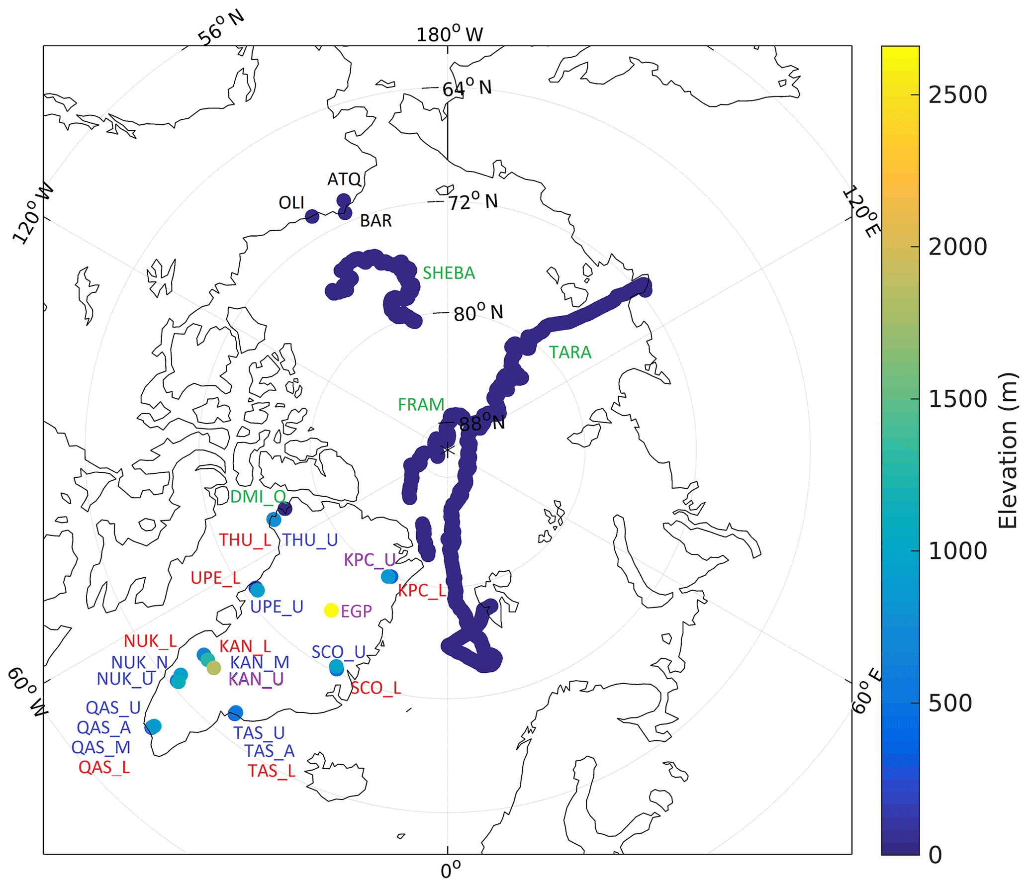
Figure 1Spatial coverage and elevation for each site included in this study. Each surface type group has been labelled with a different colour: ACC sites are purple, UAB sites are blue, LAB sites are red, SSC are black and SICE sites are green. The colour bar is elevation above sea level in metres.

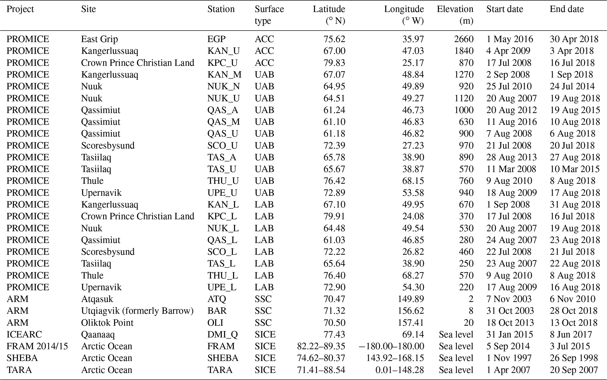
Table 1Observation sites used in this study covering the following surface types: accumulation zone (ACC), upper–middle ablation zone (UAB), lower ablation zone (LAB), seasonal snow cover (SSC) and sea ice (SICE).
2.1 PROMICE
Data have been obtained from the Programme for Monitoring of the Greenland Ice Sheet (PROMICE) provided by the Geological Survey of Denmark and Greenland (GEUS). PROMICE was initiated in 2007 by the Danish Ministry of Climate and Energy and operated by GEUS in collaboration with the National Space Institute at the Technical University of Denmark and Asiaq (Greenland Survey; e.g. Ahlstrøm et al., 2008). PROMICE collects in situ observations from a number of AWSs mostly located along the margin of the GrIS (Fig. 1). Each observational site has one or more stations, typically one located in the lower ablation zone close to the ice sheet margin and one or two located in the middle–upper ablation zone near the equilibrium line altitude. Exceptions are KAN_U and KPC_U located in the lower accumulation area and EGP, which is located in the upper accumulation area. All 22 PROMICE AWSs located on the GrIS have been used in this study. PROMICE Tskin has been calculated from upwelling longwave radiation, measured with a Kipp & Zonen CNR1 or CNR4 radiometer, assuming a surface longwave emissivity of 0.97 (van As, 2011). The air temperature is measured by a thermometer at a height of 2.7 m, while the wind speed is measured at about 3.1 m in height, if no snow is present. Snow accumulation during winter reduces the measurement height. Data where the surface albedo is less than 0.3 indicate that the snow and ice have disappeared and these data have been excluded to ensure that we only consider snow-/ice-covered surfaces. In this study, we use hourly averages of the data, provided by PROMICE.
2.2 ARM
The Atmospheric Radiation Measurement (ARM) program (Ackerman and Stokes, 2003; Stamnes et al., 1999) was established in 1989 and it provides data on the cloud and radiative processes at high latitudes. Three ARM sites from the North Slope of Alaska (NSA) are used in this study: Atqasuk (ATQ), Utqiagvik (formerly Barrow) (BAR) and Oliktok Point (OLI). The stations provide surface snow IR temperature measured using a Heitronics KT19.85 IR radiation pyrometer (Moris, 2006) and air temperature measured at 2 m in height. Wind speed is measured at 10 m in height. All measurements are provided with a sampling interval of 1 min. The ARM stations have seasonal snow coverage; i.e. the snow melts away in summer. As for the PROMICE stations, data with a surface albedo of less than 0.3 have been excluded. The data used here are thus biased towards autumn, winter and spring with 92 % of all observations being measured during the months of September–May (all three SSC sites weighted equally).
2.3 ICEARC
We use the ICEARC sea ice temperature and radiation data set from the Danish Meteorological Institute (DMI) field campaign in Qaanaaq. The DMI AWS is deployed on first-year sea ice in Qaanaaq and is funded by the European climate research project, ICE-ARC. The AWS was deployed for the first time in late January 2015 at the north side of the fjord Inglefield Bredning and recovered in early June before breakup of the fjord ice. The campaign has been repeated every year since then and the data used in this study are procured by fieldwork performed in the period of January–June 2015–2017. The AWS is equipped to measure snow surface IR temperature and air temperature at 1 and 2 m heights. In this study, the 1 m air temperature is used instead of the 2 m air temperature, as careful analysis of the 2 m air observations revealed anomalies that could arise from a systematic temperature-dependent error. Using the 1 m instead of 2 m air temperature observations will have an impact on the strength of the relationship with the Tskin observations, but the observations are included here as the dependency with other parameters, such as cloud cover and wind, is still important to assess. The data used here are snapshot measurements every 10 min (Høyer et al., 2017) and are referenced as DMI_Q in this paper.
2.4 SHEBA
The Surface Heat Budget of the Arctic (SHEBA) experiment was a multi-agency program led by the National Science Foundation and the Office of Naval Research. The data used in this study originate from deployment of a Canadian icebreaker, Des Groseilliers, in the Arctic ice pack 570 km northeast of Prudhoe Bay, Alaska, in 1997 (Uttal et al., 2002). During its year-long deployment, SHEBA provided atmospheric and sea ice measurements from the icebreaker and the surrounding frozen ice floe. The data used here contain hourly averaged data collected by the SHEBA Atmospheric Surface Flux Group (ASFG) and James C. Liljegren from the ARM project. The SHEBA ASFG installed a 20 m tall tower, which was used to obtain measurements of the surface energy budget, focusing on the turbulent heat fluxes and the near-surface boundary layer structure (Bretherton et al., 2000; Persson, 2002). The mast contains five different levels, varying in height from 2.2 to 18.2 m, on which temperature and humidity probes and a sonic anemometer are mounted. The air temperature and wind data used here originate from the lowest mounted instruments (2.2 m), which vary in height from 1.9 to 3 m depending on snow accumulation and snowmelt. Three different methods to measure surface temperature were deployed: a General Eastern thermometer, an Eppley radiometer and a Barnes radiometer, for which data are available over the period from April to September 2007. According to ASFG, the Eppley radiometer is the most reliable, though there are periods when the other two are also reasonable and one period (May) when the Eppley data may be slightly off (Persson, 2002). They provide an estimate of Tskin, which is based on slight corrections to the Eppley temperatures and the Barnes temperatures when Eppley was known to be wrong (Persson, 2002). We use the processed data from the SHEBA ASFG (Persson, 2002).
2.5 FRAM 2014/15
The scientific program of the FRAM 2014/15 expedition is carried out by the Nansen Center (NERSC) in co-operation with the Alfred Wegener Institute; Helmholtz Centre for Polar and Marine Research, Germany, University of Bergen; Bjerknes Center for Climate Research and Norwegian Meteorological Institute. FRAM 2014/15 is a Norwegian ice drift station deployed near the North Pole in August 2014 using a hovercraft as the logistic and scientific platform (Kristoffersen and Hall, 2014). This type of mission allows exploration of the Arctic Ocean not accessible to icebreakers and enables scientific field experiments, which require physical presence. By the end of March 2015 they had drifted 1450 km. During the drift with sea ice they obtained Tskin measurements using a Campbell Scientific IR120 (later corrected for sky temperature and surface emissivity) mounted on the hovercraft and near-surface air temperature measurements, with a sampling interval of 1 min.
2.6 TARA
Tara is a French polar schooner that was built to withstand the forces of Arctic sea ice. In late August 2006 Tara sailed to the Arctic Ocean, where she drifted for 15 months frozen into the sea ice. The TARA multidisciplinary experiment was part of the international polar year DAMOCLES (Developing Arctic Modelling and Observing Capabilities for Long-term Environmental Studies) program (Gascard et al., 2008; Vihma et al., 2008). Air temperature and wind speed were measured from a 10 m tall Aanderaa weather mast at heights of 1, 2, 5, and 10 m and wind direction was measured at 10 m in height. We use the air temperatures and wind speed measured at 2 m in height. They also deployed an Eppley broadband radiation mast with two sensors for longwave fluxes and two sensors for shortwave fluxes (upward and downward looking). The downward-looking IR sensor also provided Tskin from April to September 2007. The data used in this study are 10 min averages.
2.7 Radiometric observations of Tskin
The Tskin observations used in this study are all derived from radiometric observations, but with spectral characteristics that range from the Heitronics KT19.85 with a spectral response function of 9.5–11.5 µm to the Campbell Scientific IR120 with a 8–14 µm spectral window to broadband longwave observations from ∼4–40 µm. The emissivity of the ice surface varies for the different spectral windows for the radiometers and this will lead to a difference in observed Tskin as radiation from surfaces with emissivities <1 will include (one emissivity) reflected radiation from the sky. The radiation emitted from a cold sky during cloud-free conditions will thus result in a colder Tskin observation for surfaces with lower emissivities, compared to high-emissivity surfaces, and this may introduce a Tskin difference among radiometers with different spectral windows. However, ice and snow surfaces generally have very high emissivities, which reduce the effects from the reflected sky radiation. In Høyer et al. (2017), the difference in emissivity between the KT15.85 and the IR120 was modelled using an IR snow emissivity model with the spectral response functions for the two types of instruments (e.g. Dozier and Warren, 1982). This resulted in averaged emissivities of 0.998 for the KT15.85 and 0.996 for the IR120 spectral windows for a typical snow surface and an incidence angle of 25∘. Using the same approach for a broadband 4–40 µm spectrum resulted in an emissivity of 0.997. The high emissivities for all three instruments mean that the contributions from the sky are small. For realistic conditions in the Arctic, this introduces an average difference of 0.06 ∘C between the IR120 and the KT15.85 radiometer (which has a similar spectral response function as the KT19.85), with the IR120 being colder than the KT15.85 (Høyer et al., 2017). It is thus clear that the KT15.85 is closest to the true Tskin due to the high emissivity but also that these Tskin variations due to different spectral windows can be neglected.
Several of the stations (ATQ, BAR, OLI, DMI_Q, SHEBA and FRAM) used here observed both narrowband and wideband IR observations of the ice surface. The two types of Tskin have been calculated and compared for each of the stations. Figure 3 shows an example of a comparison of the two Tskin estimates from DMI_Q, showing a correlation of 0.99 and a bias of 0.69 ∘C when comparing the two Tskin estimates. There is a good relation between the two observations for the full range of temperatures, meaning that there are no temperature dependencies in the comparison. Considering all sites, a good agreement is found with a small mean difference between the two Tskin types of 0.06 ∘C and a mean root-mean-squared value of 0.96 ∘C. In the following we use the narrowband Tskin observations when available and the broadband at the other stations, and we assume that all the Tskin-derived observations have the same characteristics.
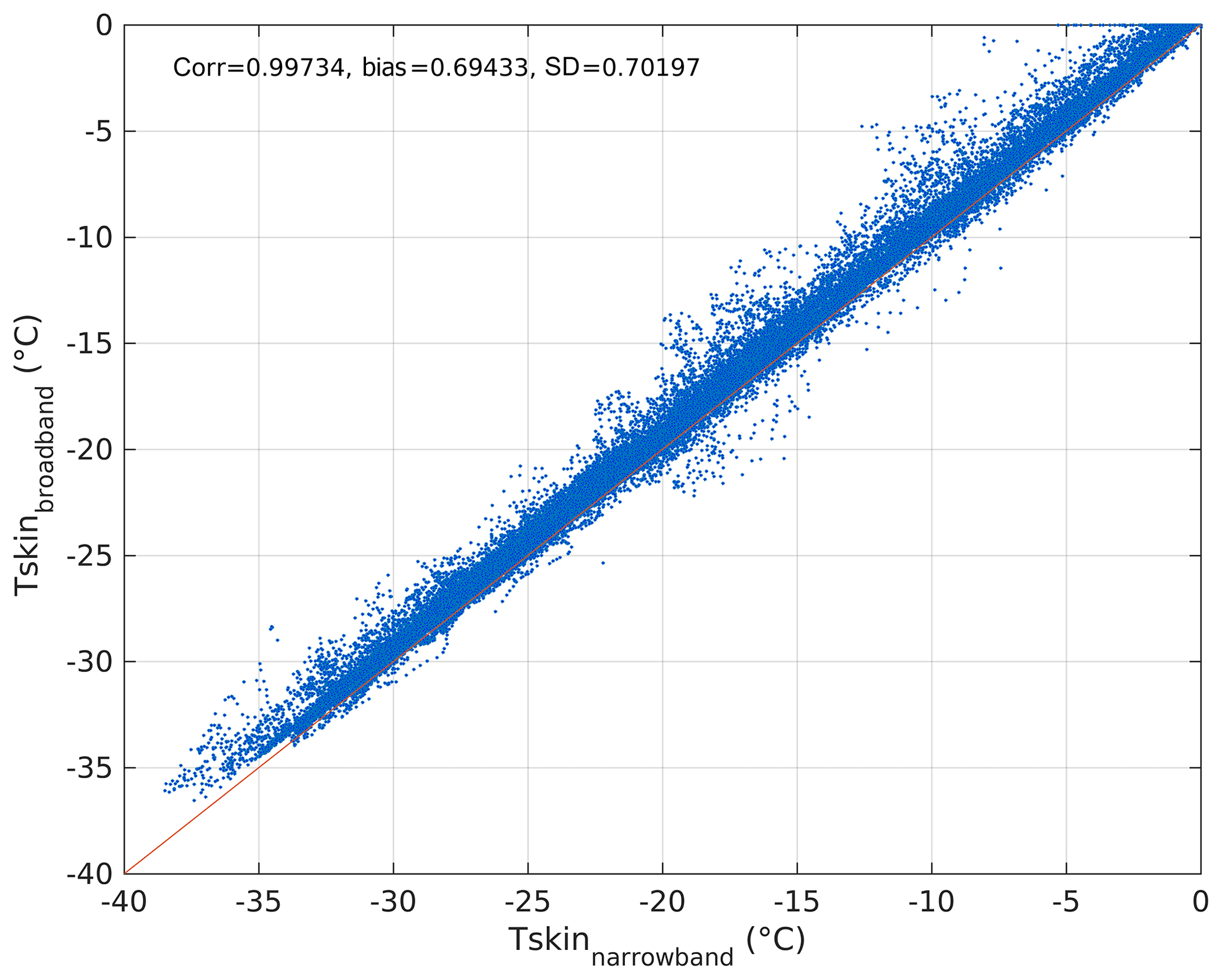
Figure 3Scatter plot of Tskin estimated from narrowband IR observations versus Tskin estimated from broadband IR observations for DMI_Q.
2.8 Longwave-equivalent cloud cover fraction
For all observation pairs, the longwave-equivalent cloud cover fraction (CCF) has been estimated based on the relationship between T2 m and downwelling longwave radiation (LWd), following the cloud cover estimation already included in the PROMICE data sets (van As, 2011; van As et al., 2005). It is based on the work of Swinbank (1963), who developed a simple approach for estimation of clear-sky (CCF =0) atmospheric longwave radiation as a function of T2 m:
where σ is the Stefan–Boltzmann constant. Overcast conditions (CCF =1) are assumed to occur when the observed LWd exceeds the blackbody radiation emitted from the surface, which is calculated using T2 m. The CCF for any observed T2 m and LWd pair from all individual observation sites is then calculated by linear interpolation of the observed LWd, between the theoretical clear-sky (from Eq. 1) and the overcast estimates. See van As (2011) for more details on the CCF calculation.
To perform an analysis of the Tskin and T2 m relationship and interpret the following results, it is important to consider the surface energy balance and the specific surface characteristics that apply in the Arctic. The surface temperature and surface melt are driven by the surface energy balance. The surface energy balance is the sum of the energy fluxes between the atmosphere and the snow–ice surface and the sub-surface land, snow–ice or ocean. The surface energy balance can be written as
where M is the net energy flux at the surface and SWd, SWu, LWd, LWu, SH, LH, and G represent the downwelling and reflected (at the surface) shortwave radiation, down- and upwelling longwave radiation, sensible and latent heat flux, and subsurface conductive heat flux, respectively. The energy fluxes have the unit watts per square metre. All fluxes are defined positive when energy is added to the surface. The surface is a skin layer, which is an infinitesimal thin layer without heat capacity, and there is an instantaneous balance among the different fluxes. This means that the elements in the surface energy balance are balanced and M equals 0 if there is no phase change (melt or refreeze). The warming or cooling of the medium below the surface affects the surface temperature through G and LH release when refreezing occurs. This affects the temperature of the medium and with that the temperature gradient close to the surface and thus G at the surface. The radiative budget of sea ice is dominated by net longwave radiation flux during much of the year. Even during summer the net shortwave radiation flux is on the same order of magnitude as the net longwave radiation flux because of extensive cloud cover, especially during late summer, and the high surface albedo of the snow (Maykut, 1986). However, SWd is the dominating source for ice melt in Greenland (van den Broeke et al., 2008; Box et al., 2012; van As et al., 2012), even though turbulent energy fluxes can dominate during shorter periods (Fausto et al., 2016). The latter is related to the fact that on average, the turbulent fluxes are an order of magnitude smaller than the radiation fluxes, and since the net radiation flux is small compared to the individual radiation fluxes, the variations in SH and LH fluxes are important for the total surface energy balance and thus the surface temperature. The turbulent mixing of the lower atmosphere increases as a function of wind speed (van As et al., 2005).
During clear-sky conditions, when SWd is negligible, LWu is higher than LWd. This results in a negative radiative balance cooling the surface and this drives a positive sensible heat flux. When the heat conduction flux from below the surface is limited on thick sea ice and on continental ice sheets, the negative radiation balance at the surface makes the surface temperature colder than the surface air temperature, resulting in a surface-based temperature inversion (Maykut, 1986). At low to moderate wind speeds, when turbulent mixing is limited, this creates a very stable stratification of the lower atmosphere. On a sloping surface, the surface air starts to flow downslope, driven by the existence of a horizontal temperature gradient and gravity. The generated winds are called inversion or katabatic winds and are characterised by stronger winds at more negative surface net radiation and a strong correlation between slope and wind direction (Lettau and Schwerdtfeger, 1967). In this paper, these winds will be referred to as katabatic winds. Clouds play a complex role in the Arctic surface energy budget. For example, they reflect SWd, leading to a cloud shortwave cooling effect, and absorb LWu and emit LWd, which tends to have a warming effect. In the Arctic, clouds have a predominantly warming effect on the surface (Intrieri, 2002; Walsh and Chapman, 1998) as the dry atmosphere, with lower emissivity and with absorptivity to LW radiation, enhances the cloud longwave warming effect, while the high surface albedo and the high solar zenith angles reduce the impact of the cloud shortwave cooling effect (Curry et al., 1996; Curry and Herman, 1985; Zygmuntowska et al., 2012).
4.1 Diurnal and seasonal temperature variability
The local air and surface temperature conditions in the Arctic are to a large extent influenced by the length of the day or night, with extreme variations depending on latitude and time of the year. In this study we will focus on the diurnal and seasonal temperature variations, as these are key temporal scales of variability and therefore important to understand when the aim is to derive T2 m from satellite observations. As an example of the large seasonal variations, Fig. 4 shows the 2014 monthly mean diurnal temperature variation in Tskin and T2 m at the upper PROMICE site in Kangerlussuaq, Greenland (KAN_U), during January, April, July and October. The seasonal variability in the diurnal temperature at KAN_U is representative of the conditions at the other stations, except for the general temperature level at each station, which changes with latitude and altitude. At KAN_U both Tskin and T2 m reach a maximum in July, while the coldest month is December (not shown) during 2014. During winter and polar night, Fig. 4 shows no clear diurnal cycle in T2 m or Tskin, and T2 m is higher than Tskin. However, during spring there is a strong diurnal cycle, with Tskin lower than T2 m at night and small T2 m–Tskin differences during daytime. The shadings indicate the standard deviations in T2 m and Tskin. The largest variability is found in spring and winter as a result of more frequent and rapid passages of cold and warm air masses in contrast to the summer months (Steffen, 1995). The summer temperature variability is moreover limited by the upper limit of 0 ∘C on Tskin during surface melt. Considering all months individually, there is high correlation between Tskin and T2 m, ranging from an average value of 0.92 in January to an average of 0.99 in July considering the entire time series of KAN_U, 2008–2018. The high correlations arise from hourly variability and daily cycles in temperatures that are seen in both temperature records. The correlation decreases for stations which have occasional surface melt, where Tskin is constrained to the freezing point of water. The presence of a lower Tskin compared to T2 m is a general phenomenon found for all stations. Tskin is thus lower than T2 m 85 % of the time, when all sites are weighted equally, whereas the opposite is true for only 13.7 % of the observation times.

Figure 4Mean diurnal variability of 2 m air temperature (T2 m) and skin temperature (Tskin) at KAN_U during the months: January, April, July and October 2014. The orange lines are the temperature difference T2 m–Tskin. The shadings indicate the standard deviations, which represent the variability in the monthly mean.
The large seasonal variations in Fig. 4 and the relationship between T2 m and Tskin are typical for all sites. Figure 5a shows the monthly mean Tskin for all sites and all years. EGP is by far the coldest site due to its high elevation, with a monthly mean Tskin of −42 ∘C in January and a maximum of −11 ∘C in July. All sites reach a maximum in Tskin in July, regardless of latitude. July is also the month with least variation in temperature among sites, where melt at most stations (exceptions are the ACC sites) constrains Tskin, while the winter months show a larger variance in Tskin among sites since local conditions dominate Tskin. The AWS data from the GrIS show the effect of altitude and latitude on Tskin, with the high-altitude sites being the coldest (EGP, KAN_U and KAN_M) together with the most northern sites (THU_U and KPC_U). The southern (e.g. QAS_A and QAS_U) and low-altitude sites (most LAB sites, TAS_U and TAS_A) are the warmest. The SICE sites are comparable in temperature with the coldest sites on the GrIS (except EGP) but are slightly warmer in summer and autumn.
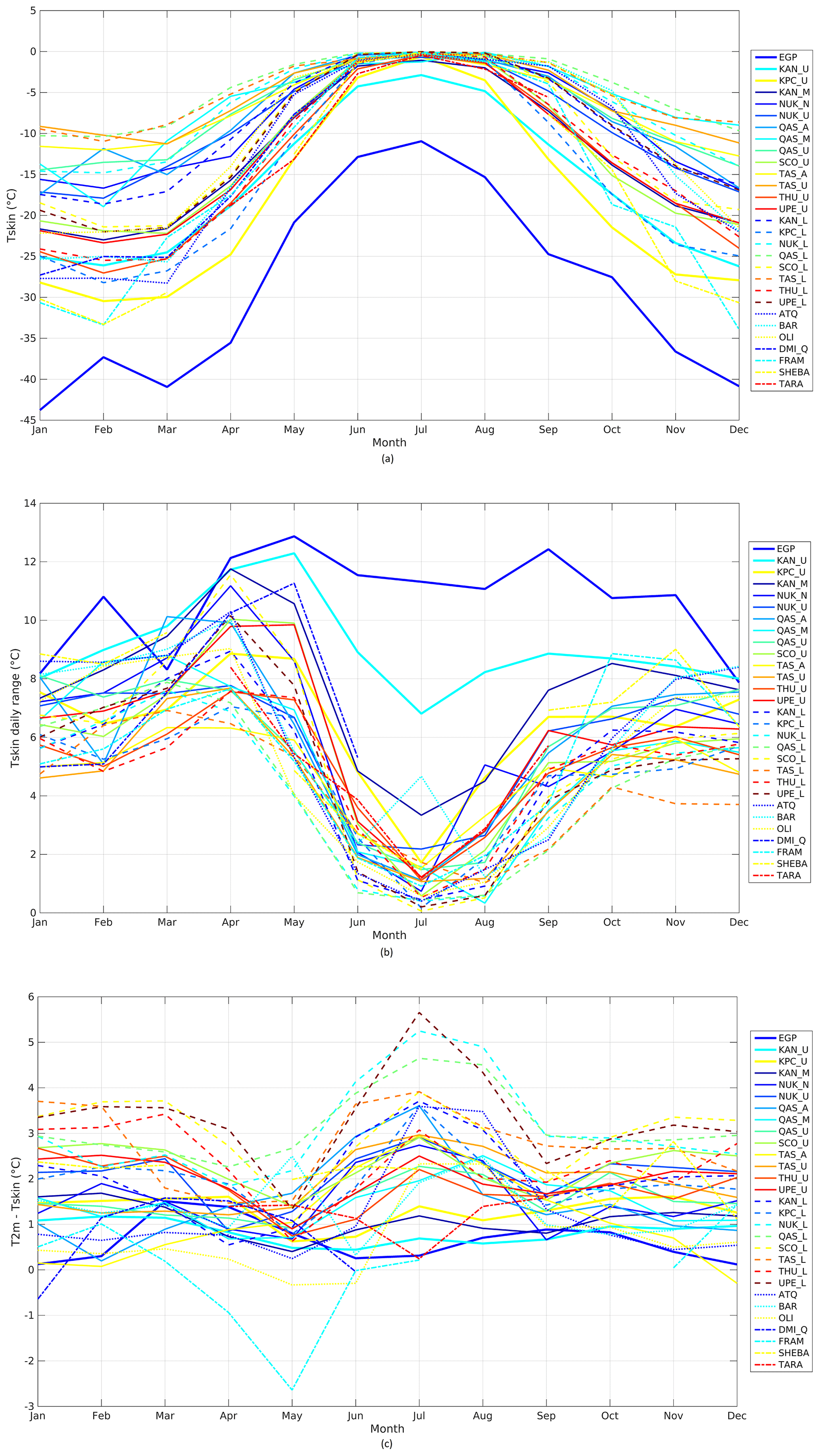
Figure 5Monthly mean Tskin (a), daily range in Tskin (b) and T2 m–Tskin difference (c) for all sites. Each surface type has its own line style or line width. See Table 1 for station locations and types.
Figure 5b shows the mean daily range (daily max–daily min difference) of Tskin as a function of month for all sites and all years. Again, the observations show a similar pattern across the diverse geographical locations. During summer, the high-elevation sites tend to have the largest daily range in Tskin, while the observations from LAB and SICE sites show the smallest daily range. This is mostly an effect of the warmer temperatures and the Tskin upper temperature limit at 0 ∘C, the melting point for ice. This constraint is seen during summer in almost all data records included in this study (exceptions are the ACC sites). Figure 5c shows the monthly mean difference between T2 m and Tskin for all observation sites as a function of time of year. The T2 m–Tskin differences observed in Fig. 5c have been averaged for each surface type category in Table 2, divided into summer months (June–August), winter months (December–February) and all available months. Note that DMI_Q is withheld from the averaging for the SICE sites to avoid systematic impacts from the 1 m height observations used from DMI_Q. In general, the ACC, SSC and SICE sites show the weakest inversion, while the UAB and LAB sites show the strongest inversion. For the ACC sites the weakest inversion is found during summer, while the UAB and LAB sites have the strongest inversion during summer. This is explained by the UAB and LAB sites having surface melt in contrast to the high-elevation ACC sites, where the surface warms but does not reach the upper limit at the melting point.
Table 2Overall 2 m air temperature and skin temperature differences (T2 m–Tskin, ∘C) for each surface type for different seasons and sky conditions. All months refer to the full time series as given in Table 1. The square brackets are the ranges of the T2 m–Tskin, differences for the stations included in each surface type category. The DMI_Q site is excluded from the SICE averages.
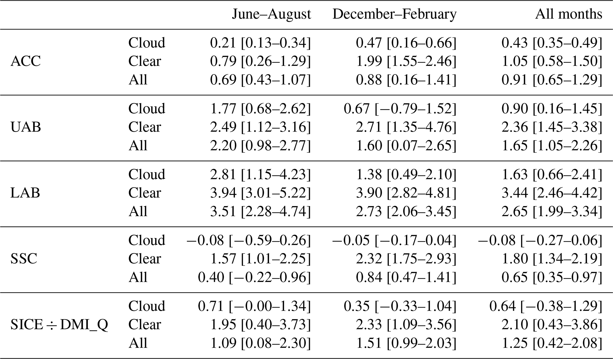
The SSC sites also experience melt, but the snow melts away in summer, which limits the time when Tskin is constrained to the melting point. It is difficult to interpret the seasonal dependencies for the SICE sites, as none of the individual sites cover an entire year. Figure 5 indicates both seasonal and daily variations in the observed Tskin and T2 m relationship. Figure 6a and b illustrate the mean diurnal and seasonal T2 m–Tskin differences for the ACC and LAB sites, respectively. The SSC and SICE sites have not been included as none of the individual sites have a continuous data record throughout the year. Figure 6a and b indicate that the winter months have very little diurnal variability in the T2 m–Tskin difference (as is also evident in Fig. 4), with an approximately constant difference of about 1.5–2.5 ∘C for the LAB sites and 0.5–1.5 ∘C for the ACC sites. During spring and summer the differences decrease at the ACC sites and the weakest vertical stratification is found around noon or early afternoon, where Tskin may even exceed T2 m slightly, resulting in an unstable stratification of the surface air column. For the LAB sites, the weakest stratification is found in spring and autumn, around noon and early afternoon. The summer months show large T2 m–Tskin differences due to the constrain of Tskin for melting surfaces, which is common to all LAB sites. At night the net radiation is typically negative, thus cooling the surface and resulting in a surface-based inversion for both surface types. The T2 m–Tskin differences are higher (especially in summer) at the LAB sites compared to the ACC sites, and the UAB sites have temperature differences in between. The reason for the higher temperature difference at the lower-altitude sites is the longer time periods with surface melt, which is due to higher temperatures.
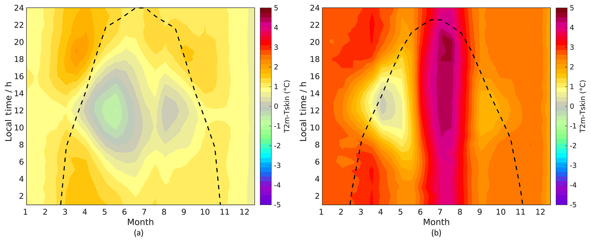
Figure 6Mean difference between 2 m air temperatures (T2 m) and skin temperatures (Tskin) for (a) ACC and (b) LAB sites as a function of time of year (with a bin size of 15 days) and local time of the day. The dotted lines indicate the maximum number of sunlight hours each month. All sites in each surface type category are weighted equally.
As mentioned in Sect. 2, the measurement height changes with snowfall and snowmelt and with the strength of the inversion measured. The PROMICE data include a height of the sensor boom, which can be used to determine the impact of using different measurement heights on our results. We reproduced the numbers in Table 2, based upon observations measured at a height of 1.9–2.1 m only and found over all all-sky, all-month differences less than 0.22 ∘C for all the different PROMICE regions. In addition, the screening did not change the conclusions regarding the impact of clouds and the seasonal behaviour of the T2 m–Tskin differences. Data from the other sites do not all include such information on the measurement height. For consistency, we therefore chose not to screen the PROMICE data. In addition, we chose not to perform an adjustment of the observations, as we estimate the uncertainty of such an adjustment to be equal to or larger than the uncertainty in the results obtained here.
4.2 Impact by wind
The surface wind speed is an important component in the near-surface thermal stratification since the turbulent mixing increases as a function of wind speed (Monin and Obukhov, 1954). Figure 7 shows how the wind regimes differ among the observation sites used in this study. In general, winds on the GrIS are strongest in winter and reach a minimum around July (see also Steffen and Box, 2001). The surface radiative cooling and the terrain play the primary role in the generation of the surface winds. The direction and strength of the prevailing surface winds are closely related to the direction and steepness of the slope and the strength of the inversion. Surface winds at the PROMICE sites generally have a high directional persistence (see Fig. 4 in van As et al., 2014), commonly blowing from inland, which is an indication that local winds are often of katabatic origin. High-elevation sites experience stronger winds due to the larger radiative cooling of the surface (provided a comparable surface slope is present; Fig. 7; van As et al., 2014). The SSC and SICE sites show less variability in wind speed on an annual basis. At these sites the wind is determined by large-scale synoptic conditions combined with local topography.
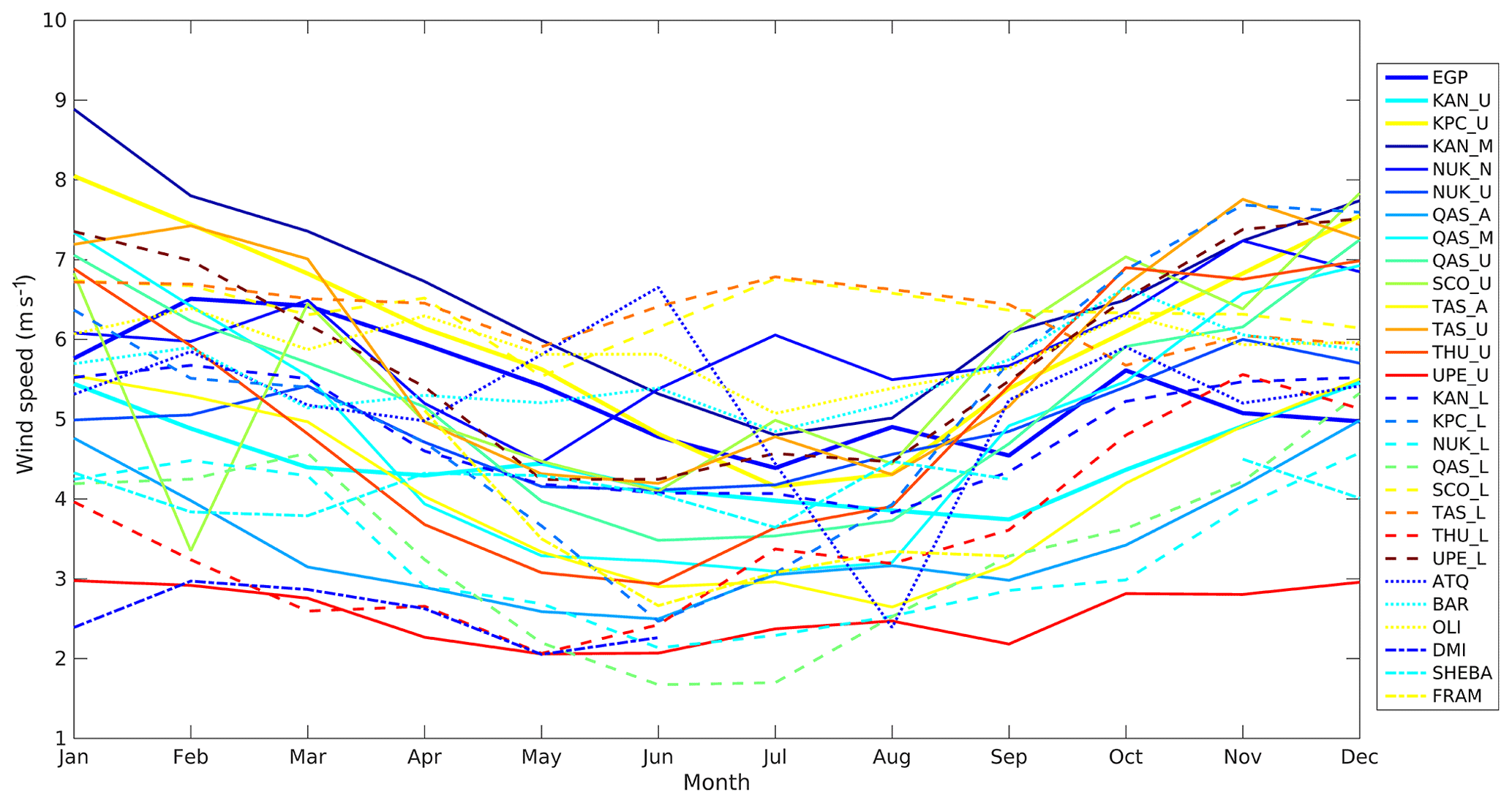
Figure 7Monthly mean wind speed (m s−1) for all sites. Each surface type has its own line style or line width. See Table 1 for station locations and types.
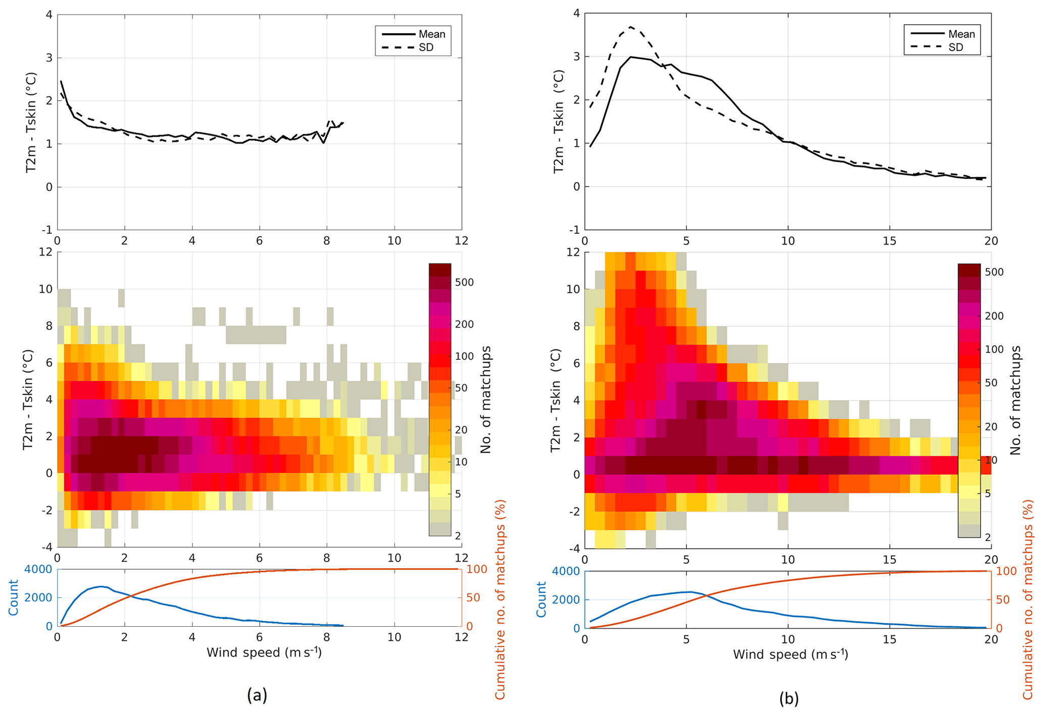
Figure 8The 2 m air temperature (T2 m) and skin temperature (Tskin) difference as a function of binned wind speed for (a) DMI_Q (SICE site) and (b) THU_U (UAB site). The wind speed bin size is 0.5 m s−1, the T2 m–Tskin bin size is 1 ∘C and only bins with more than 50 members are included. The upper plots show the standard deviation (dashed lines) and mean difference (solid lines). The middle plots show the number of members in each bin while the bottom plots show the number of members (blue lines) and the cumulative percentage of members (red lines) in each wind speed bin.
The expectation is that stronger inversions can develop in low wind speed conditions because of reduced turbulent mixing. Figure 8a and b show the T2 m–Tskin difference as a function of wind speed for selected sites. The top plots show the mean (solid lines) and standard deviation (dashed lines) of the T2 m–Tskin difference as a function of wind speed. Figure 8a shows data from the DMI_Q AWS on sea ice. As expected, the strongest temperature inversion occurs at low wind speeds, and larger wind speeds have larger turbulent mixing and thus smaller vertical temperature differences between Tskin and T2 m. However, data from THU_U (Fig. 8b) show that this relationship is more complex. The maximum inversion is reached at wind speeds from 3 to 5 m s−1, whereas the mean and standard deviation decrease for calm winds (<2.5 m s−1).
The wind dependencies shown in Fig. 8 are representative for all the stations in this paper, for which the SICE and the SSC sites resemble Fig. 8a and all the PROMICE stations have a wind dependency similar to Fig. 8b. The pattern of the PROMICE stations is explained by the combination of inversion and a surface slope that results in a flow, which reduces the strength of the inversion (its own forcing). For large wind speeds the inversion will be destroyed and calm winds can only occur when the inversion is close to zero (as the presence of inversion on sloping surfaces forces a wind). As a result there is an optimum in inversion strength and wind speed, which in this case is at wind speeds of 3–5 m s−1. This behaviour is also found by Adolph et al. (2018) at the Summit station on the GrIS. Miller et al. (2013) also found that the surface-based inversion intensity peaks at wind speeds ranging from 3 to 10 m s−1 at Summit based on microwave-radiometer-retrieved profiles. Furthermore, Hudson and Brandt (2005) show that at the South Pole the maximum inversion strength occurs at wind speeds of 3–5 m s−1. They investigated this using the model by Mahrt and Schwerdtfeger (1970) and their results supported the idea that the inversion forces an air flow, which can explain the “unexpected” location of the maximum in inversion strength. The nature of the surface winds and the directional constancy are highly comparable between the sloping surfaces of Antarctica and Greenland (van den Broeke et al., 1994; King and Turner, 1997) and in both cases the maximum inversion occurs at non-zero wind speeds.
4.3 Impact by clouds
The difference in LWd radiation between clear-sky and overcast conditions can result in large differences in both T2 m and Tskin due to the cloud effect on the surface radiation budget. As IR satellite Tskin can only be retrieved during clear-sky conditions, the assessment of the cloud effect on the average conditions is essential to facilitate the combination of satellite and in situ observations. In this section, we therefore assess the inversion strength as a function of the cloud cover and in the next section the clear-sky bias is estimated for all sites.
Clear-sky conditions are defined to be cases in which CCF <0.3, while overcast conditions are defined to have CCF >0.7. The frequency of clear-sky (overcast) observations is defined as the number of clear-sky (overcast) observations compared to the total number of observations. Figure 9 shows the frequency of clear-sky and overcast observations for each of the observation sites used in this study. The SSC and SICE sites and EGP all show a much larger frequency of overcast conditions compared to the frequency of clear-sky conditions. Also, the TAS_U, TAS_A and TAS_L sites located in the high-accumulation area (Ohmura and Reeh, 1991) of the southeastern part of the GrIS tend to have more overcast observations compared to clear-sky observations. There is a general tendency with more frequent overcast observations for increasing altitudes for the PROMICE sites. The ACC sites have a strong seasonal dependence with more clear-sky observations during summer and more overcast conditions during winter (not shown). A similar but much weaker seasonal cycle is seen for UAB. The LAB and SSC sites show limited seasonal variability, while the SICE sites have almost no clear-sky observations during the months from August to March (not shown).
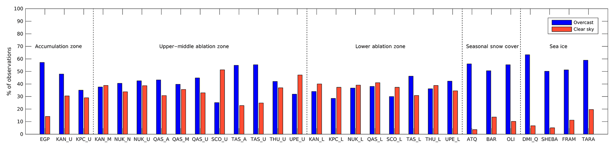
Figure 9Frequency of clear-sky and overcast observations as percentages of all observations for each site.
The relation between the inversion strength and CCF is shown in Fig. 10 for all sites. As expected, the inversion strength decreases for larger cloud cover fractions due to increasing LWd radiation. For each surface type category the average slope has been calculated based on linear fits to the graphs in Fig. 10: ACC ∘C %−1, UAB ∘C %−1, LAB ∘C %−1, SSC ∘C %−1 and SICE ∘C %−1, for which the uncertainties are given as 95 % confidence intervals on the slope values. The average r2 fit values for each surface type category are 0.25 (ACC sites), 0.76 (UAB sites), 0.83 (LAB sites), 0.55 (SSC sites) and 0.40 (SICE sites). Excluding ATQ and EGP (with very low r2 values of 0.013 and 0.0014, respectively) increases the average r2 to 0.83 and 0.38 for SSC and ACC sites, respectively. These results indicate that a linear approximation is a good assumption for UAB, LAB and SSC (excluding ATQ), whereas the ACC and SICE dependencies are further away from linear.
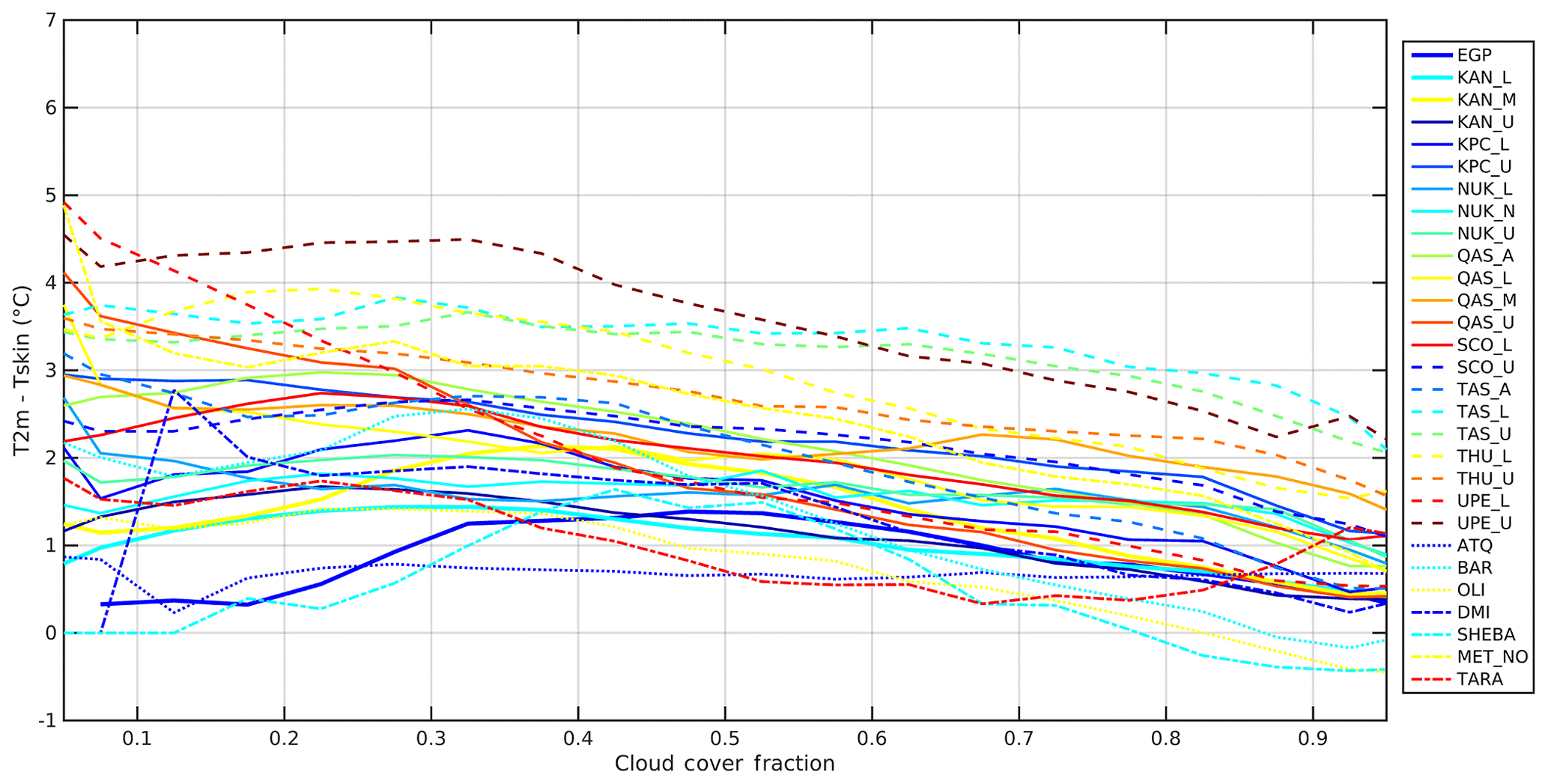
Figure 10The 2 m air temperature and skin temperature differences for all sites as a function of binned cloud cover fraction (CCF). The CCF bin size is 0.05, the T2 m–Tskin bin size is 1 ∘C and only bins with more than 50 members are considered. Each surface type has its own line style or line width.
Figure 11a and b show how the temperature differences at the ACC sites vary as a function of season and local time for clear-sky and overcast conditions, respectively. Clear-sky conditions show the largest stratification with temperature differences up to 2–3 ∘C during winter and night-time. Overcast conditions reduce the temperature gradient at all times, with the maximum temperature differences of about 1 ∘C. During summer around noon, overcast conditions usually lead to an unstable stratification of the order of −1 ∘C. An unstable stratification may also occur during clear-sky conditions and large solar insolation. This behaviour is common for all sites included in this study, but the strength of the inversion varies among the different sites. Table 2 also summarizes the impact of clouds on the T2 m–Tskin differences for each surface type category. For all surface types and for all times of the year, cloud cover tends to decrease the inversion strength.
To assess the impact of the different spectral characteristics of the used radiometers (broadband versus narrowband, as discussed in Sect. 2.7) on the observed Tskin, the T2 m–Tskin differences were calculated as a function of CCF for both narrow- and broadband Tskin for the sites containing both instruments (ATQ, BAR, OLI, DMI_Q, SHEBA and FRAM). The average slope for the above sites was estimated in both cases and resulted in a small difference in the slope from −0.017 to −0.020 ∘C %−1 for narrowband and broadband Tskin estimates, respectively.
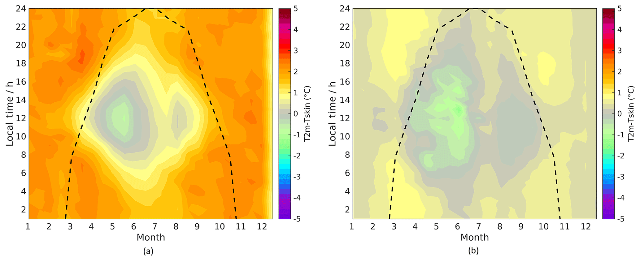
Figure 11Mean difference between 2 m air temperatures (T2 m) and skin temperatures (Tskin) for ACC sites in cases of (a) clear-sky and (b) overcast conditions. The dotted lines indicate the maximum number of sunlight hours each month. All sites in each surface type category are weighted equally.
4.4 Clear-sky bias
The most accurate surface temperature satellite observations are thermal IR observations that can only be utilized during clear-sky conditions. As the satellite IR observations thus have gaps resulting from cloud cover, the satellite Tskin products are often averages of the available satellite observations over a 1–3-day period (see e.g. Rasmussen et al., 2018). However, these satellite averages will differ from the all-sky average temperature since the Tskin is typically lower during clear-sky conditions compared to cloudy conditions. This difference is referred to as clear-sky bias. When using the averaged Tskin observations from satellites for monitoring or in combination with ocean, sea ice or atmospheric models, it is thus important to assess the impact off the different temporal averaging windows on the clear-sky bias. Hall et al. (2012) show monthly temperature maps from MODIS and discuss the fact that the monthly average temperatures (from satellites) are likely lower than the all-sky monthly average temperatures. Here, we use the in situ observations to estimate the clear-sky effects that satellite observations would introduce. We use a cloud mask derived from the longwave-equivalent cloud cover fraction and assume that it is equivalent to the cloud masks used for IR satellite processing. The clear-sky bias is assessed by comparing all available clear-sky Tskin observations (where clear sky has been defined as a CCF <0.3) with all available all-sky Tskin observations, averaged for different time windows: 24 h, 72 h and 1 month, for all sites. The three averaging windows were chosen to examine the clear-sky effect for previously used averaging windows in Rasmussen et al. (2018) (72 h) and when calculating monthly climatological values. The results are shown in Fig. 12. For most stations all-sky observations are warmer than clear-sky observations for all time windows and the difference tends to increase with increasing length of temporal averaging window. The larger clear-sky biases for longer temporal averaging windows arise from persistent cloud cover lasting for days. A clear-sky bias cannot be computed when using temporal averaging windows of shorter length than the duration of overcast conditions due to missing clear-sky observations. If however, a longer temporal averaging window is used, the Tskin observations during the overcast conditions (which tend to be warmer than during clear sky) will be included in the all-sky average. The result is a warmer all-sky Tskin for longer temporal averaging windows and thus a larger clear-sky bias. There is large variability among the stations, and at a few stations, such as EGP, KPC_U, ATQ, OLI and DMI_Q, the all-sky observations are colder than clear-sky observations using one or more of the temporal averaging windows. These positive clear-sky biases are very likely a result of seasonal differences in cloud cover.
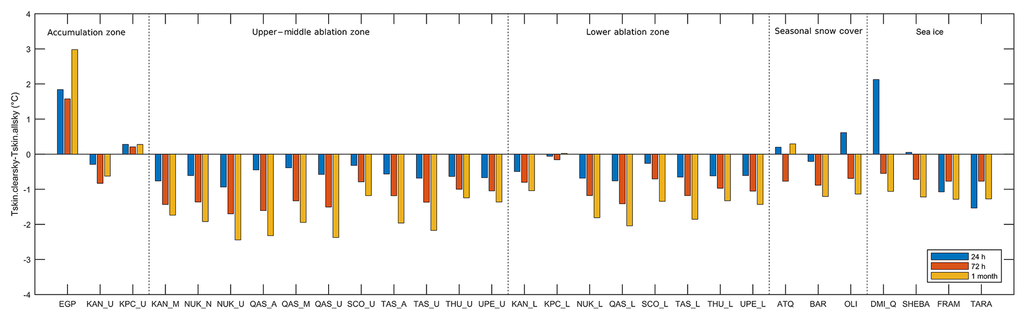
Figure 12Observed clear-sky biases (Tskin.clearsky–Tskin.allsky) averaged for different time intervals, for all sites (∘C).
Figure 13a and b show the monthly mean difference in the 24 h averaged clear-sky and all-sky Tskin for the ACC stations (a) and the LAB stations (b), together with the average number of hours with clear sky per day. For both groups of stations it is found that the 24 h averaged clear-sky bias is closest to zero during summer, which can partly be explained by the smaller daily Tskin range in summer (Fig. 5b). The UAB sites (not shown) look very similar to the LAB sites but with a slightly more pronounced seasonal cycle in the clear-sky bias. The figures have not been produced for the SSC and SICE sites as none of the individual sites included in these categories cover an entire season. Figure 13 also shows more hours with clear skies for LAB stations compared to ACC stations except for the period of May–July, when both surface groups on average have about 12 h with clear sky per day. For the ACC sites the number of hours with clear sky decreases to about 4 h per day during September–March. It is found that EGP has no clear-sky observations in December–February and at DMI_Q there are no clear-sky observations available for January–March, which means that the results in Fig. 12 are biased towards the months when a zero or positive clear-sky bias is observed. This very likely explains the positive clear-sky biases observed (in Fig. 12) for these stations. The 72 h and 1-month averaged clear-sky biases show the same seasonal variation as in Fig. 13, with the smallest biases in summer and largest biases in winter (not shown).
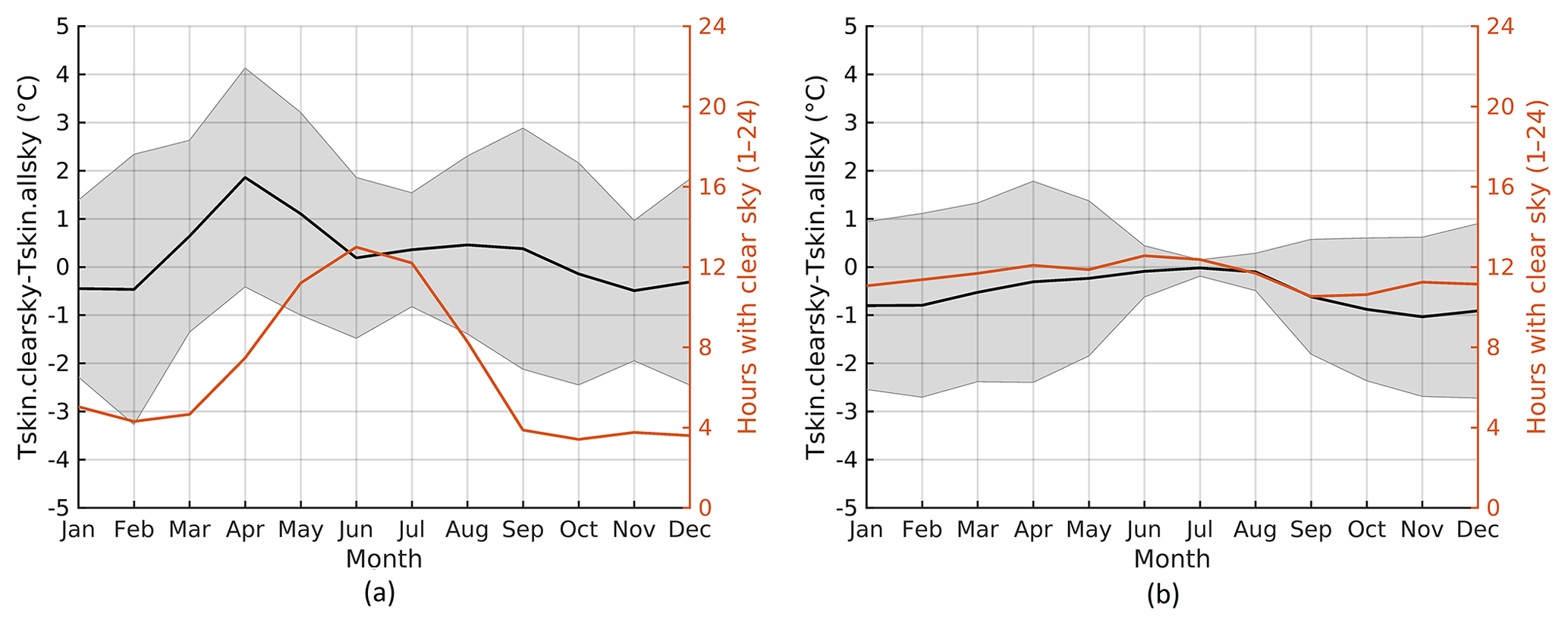
Figure 13Monthly mean differences between 24 h averaged clear-sky and all-sky skin temperatures for (a) ACC stations and (b) LAB stations. The orange lines show the 24 h average number of hours with clear sky (CCF <0.3) per day for each month. The grey bands show the monthly average of the daily standard deviations. All sites in each surface type category are weighted equally.
The observed clear-sky bias explains part of the cold bias observed in IR satellite retrievals of skin surface temperature compared to in situ skin surface temperatures as seen in Høyer et al. (2017) and Rasmussen et al. (2018). Another contribution to a satellite versus in situ cold bias is related to the fact that the satellite skin observations are compared to in situ observations measured at typically 2 m in height (Shuman et al., 2014). Temperature inversions in the lowest 2 m of the atmosphere will thus result in the satellite retrievals of surface temperature being colder than the in situ measurements at 2 m in height.
4.5 Relationship between Tskin and T2 m
Section 4.3 showed how clouds impact the T2 m and Tskin relationship, and Sect. 4.4 revealed how satellite Tskin is affected by clouds. With the aim of deriving T2 m based upon satellite Tskin observations, it is important to examine how the T2 m–Tskin difference is related to the skin temperature itself. The relationship with Tskin is shown in Fig. 14 in which the strength of the surface-based inversion is shown as a function of Tskin. All PROMICE sites show an almost linear trend towards weaker inversion strength for higher skin temperatures with the steepest slope of the curve for low-elevation sites. The average slopes of the linear fits of the graphs in Fig. 14 for all categories are found to ACC , UAB , LAB , SSC and SICE , for which the uncertainty estimates are given as 95 % confidence intervals on the slopes. The average r2 fit values for each surface type category are 0.76 (ACC sites), 0.77 (UAB sites), 0.86 (LAB sites), 0.54 (SSC sites) and 0.51 (SICE sites). The numbers demonstrate that the linear relationship is a better assumption when using Tskin compared to cloud cover fraction. The results of this section show that the slopes are similar within each region but tend to vary from region to region. This indicates that Tskin and T2 m relationship models can be derived on a regional level using Tskin for situations in which the cloud cover and longwave radiation are not available, such as the case with satellite observations.
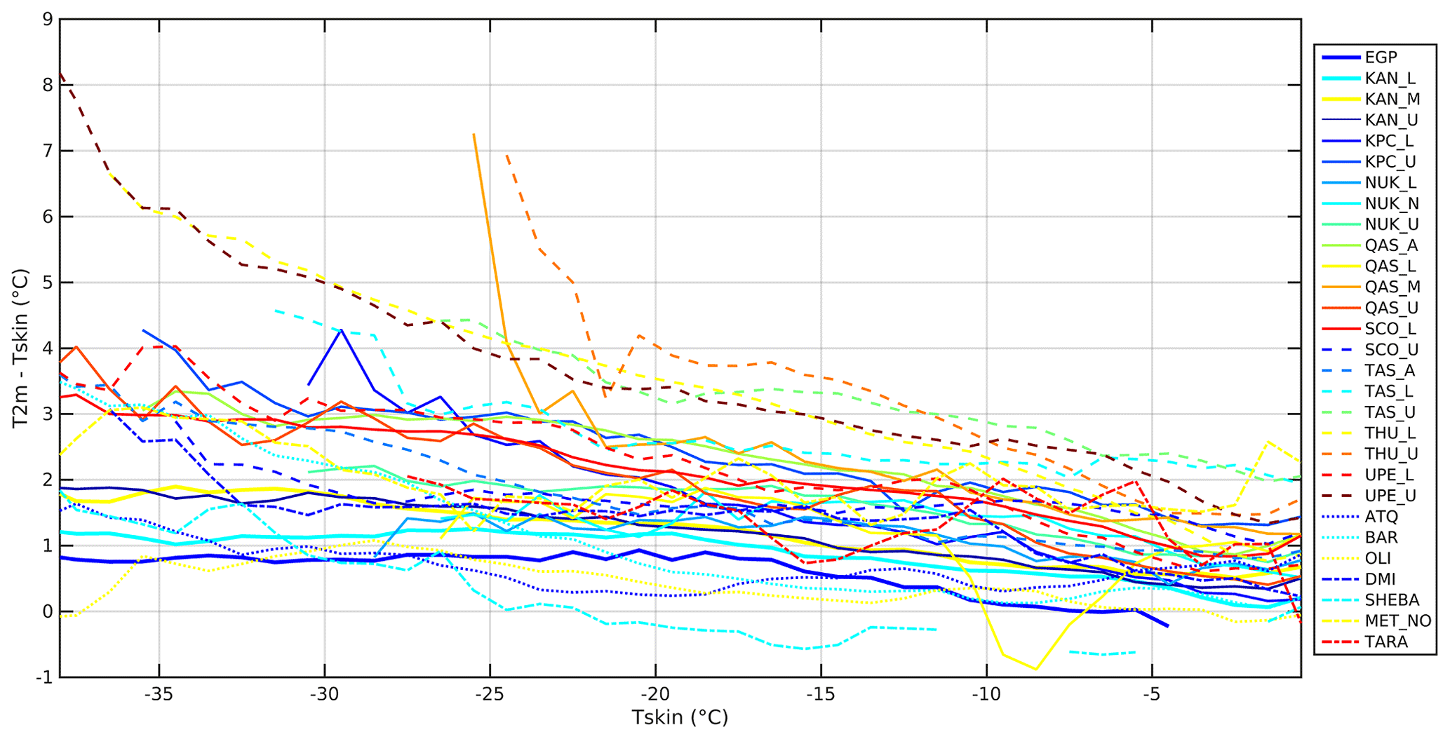
Figure 14Mean 2 m air temperature and skin temperature differences (T2 m–Tskin) for all sites as a function of binned skin temperature (Tskin). The Tskin bin size is 1 ∘C, the T2 m–Tskin bin size is 1 ∘C and only bins with more than 50 members are considered. Each surface type has its own line style or line width.
As in Sect. 4.3, the impact of the different spectral characteristics of the radiometers on the above results has been assessed. The T2 m–Tskin differences were calculated for both types of radiometers as a function of Tskin for the sites containing both instruments (ATQ, BAR, OLI, DMI_Q, SHEBA and FRAM). Again, the difference in the average slope was small, from −0.046 to −0.055 for narrow- and broadband Tskin estimates, respectively.
Coincident in situ skin temperature (Tskin) and 2 m air temperatures (T2 m) from 29 sites in the Arctic region have been analysed to assess the variability and the factors controlling the Tskin and T2 m variations. The aim is to facilitate the combined use of satellite-observed Tskin and traditional observations of T2 m. The extensive data set used in this study represents a wide range of conditions including all-year observations from Arctic sea ice, land ice in northern Alaska, and low- and high-altitude land ice covering the lower, middle and upper ablation zones and the accumulation region of the Greenland Ice Sheet (GrIS). It has been found that for each region there is a good correspondence between the Tskin and T2 m and that the main factors influencing the relationship between Tskin and T2 m are seasonal variations, wind speed and cloud cover.
Considering all surface type categories, the mean T2 m–Tskin difference is on average 0.65–2.65 ∘C, with the strongest inversion at the sites located in the lower ablation zone and the weakest inversion at the sea ice sites. Inversions are predominantly found during winter (low-sun and polar night periods), which allows for a strong radiative cooling at the surface. Smaller T2 m–Tskin differences dominate around noon and early afternoon in spring and summer, when the sun is warming the surface but no melting occurs. This is in agreement with Adolph et al. (2018), who found large T2 m–Tskin differences during night-time and small differences during the peak solar irradiance at Summit, GrIS (see Fig. 5 in Adolph et al., 2018). During local noon in spring, autumn and summer (during non-melting conditions), satellite-observed skin temperatures will therefore have the best agreement with the T2 m.
Increasing wind speeds are expected to decrease the inversion strength through increased turbulence and mixing of warmer air towards the surface. This is seen at the ARM sites and the Arctic sea ice sites, where the strongest inversion occurs at calm winds. Conversely, the inversion strength decreases with increasing wind speed. The relationship is more complicated over a sloping terrain with the maximum inversion strength at winds of 3–5 m s−1 for all the GrIS sites. This feature has previously been identified by others for Antarctica (Hudson and Brandt, 2005) and at Summit, GrIS (Adolph et al., 2018; Miller et al., 2013), and can be explained by the presence of a katabatic wind driven by the surface temperature inversion over a sloping terrain. The katabatic wind reduces the inversion strength, and as a result there is an optimum in inversion strength and wind speed.
The analysis of the impact of clouds showed an almost linear relationship between cloud cover fraction (CCF) and the T2 m–Tskin difference, with a trend towards zero with increasing CCF, for most sites (Fig. 10). Considering all surface type categories, the T2 m–Tskin difference decreases from an all-sky mean value ranging from 0.65 to 2.65 ∘C to a difference ranging from −0.08 to 1.63 ∘C for observations with a CCF above 0.7. Conversely, the T2 m–Tskin difference increases to the range of 1.05–3.44 ∘C by only considering observations with CCFs below 0.3. The smaller inversion strength under cloudy conditions is explained by the fact that clouds have a predominantly warming effect on the surface in the Arctic (Intrieri, 2002; Walsh and Chapman, 1998). In situations in which the cloud cover and longwave radiation are not available, the T2 m–Tskin relationship can be quantified by using the Tskin. We have found an almost linear relationship between the inversion strength and the skin temperatures, with weaker inversions for higher Tskin. This is in agreement with Adolph et al. (2018), who found larger T2 m–Tskin differences at lower temperatures at the Summit station during summer.
In order to facilitate the construction of a satellite-derived T2 m product, the influence of clouds on temporally averaged Tskin has been assessed. This has been performed by comparing clear-sky Tskin observations with all-sky Tskin observations averaged over different time intervals: 24 h, 72 h and 1 month. In general, the clear-sky average is colder than the all-sky average with increasing bias with the length of the averaging time interval. The clear-sky bias is smaller during summer than winter for all averaging windows. This is also reported by Comiso (2000), who finds a monthly mean clear-sky bias of about −0.3 ∘C during summer (January) and −0.5 ∘C during winter (July) at Antarctic stations. The seasonal variation in clear-sky bias in combination with differences in frequency and timing of clear-sky observations lead to differences among the stations. The average positive clear-sky bias at EGP, for example, is thus a result of persistent cloud cover during winter months and predominantly clear sky in summer months, when the clear-sky bias is small or positive.
The assessment of the T2 m–Tskin differences and the identification of the main variables that control the variability are important findings when developing a statistical model to estimate the T2 m from satellite Tskin observations. In addition, the findings in the diurnal and seasonal variations in the T2 m–Tskin differences are valuable when validating the satellite Tskin against T2 m observations. All the identified parameters can be derived from either the satellite retrievals themselves or from numerical weather prediction (NWP) analysis. The generation of a daily satellite-derived T2 m product for the polar regions using a statistical model is thus facilitated with these results, which is the focus of current developments. Such a satellite-derived product can be independent of other existing surface temperature products and NWP reanalysis and can therefore contribute significantly to improvements in Arctic climate change monitoring and assessment.
The PROMICE data can be accessed through http://www.promice.dk (last access: 16 November 2018). The ARM data are available at https://www.archive.arm.gov/discovery/\#v/results/s/s::co (last access: 21 December 2018). The SHEBA data are available from https://atmos.uw.edu/~roode/SHEBA.nc.readme.html (last access: 28 November 2017), while the DMI ICEARC data are available through the https://doi.org/10.6084/m9.figshare.7831526 (Høyer et al., 2019). The Tara data are provided through personal communication with Timo Palo from the TARA expedition. Similarly, data from the FRAM 2014/15 expedition can be obtained through personal communication with Steinar Eastwood from the Norwegian Meteorological Institute.
PNE, KSM, RT, GD and EA compiled the in situ data. PNE, JLH and KSM designed the experiments and PNE carried them out. PNE prepared the paper with contributions from all authors.
The authors declare that they have no conflict of interest.
This study was carried out as a part of the European Union Surface
Temperatures for All Corners of Earth (EUSTACE), which is financed by the
European Union's Horizon 2020 Programme for Research and Innovation, under
grant agreement no. 640171. The aim of EUSTACE is to provide a spatially
complete daily field of air temperatures since 1850 by combining satellite
and in situ observations. The author would like to thank the data providers.
Data were provided by PROMICE, which is funded by the Danish Ministry of
Climate, Energy and Building, operated by the Geological Survey of Denmark
and Greenland and conducted in collaboration with the National Space
Institute (DTU Space) and Asiaq (Greenland Survey). Data were also obtained
from the Atmospheric Radiation Measurement (ARM) Climate Research Facility, a
U.S. Department of Energy Office of Science user facility sponsored by the
Office of Biological and Environmental Research. We thank our colleagues in
the SHEBA Atmospheric Surface Flux Group, Ed Andreas, Chris Fairall, Peter
Guest and Ola Persson for help collecting and processing the data. The
National Science Foundation supported this research with grants to the U.S.
Army Cold Regions Research and Engineering Laboratory, NOAA's Environmental
Technology Laboratory, and the Naval Postgraduate School. Data were also
provided by Timo Palo from the TARA expedition, supported by the European
Commission 6th Framework Integrated Project DAMOCLES and in part by the
Academy of Finland through the CACSI project. We thank Steinar Eastwood from
the Norwegian Meteorological Institute for providing us with data from the
FRAM 2014/15 expedition. Finally, we would like to thank the anonymous
reviewers for their careful reading and their insightful suggestions and
comments, which substantially improved this paper.
Edited by: John Yackel
Reviewed by: three anonymous referees
Abermann, J., Hansen, B., Lund, M., Wacker, S., Karami, M., and Cappelen, J.: Hotspots and key periods of Greenland climate change during the past six decades, Ambio, 46, 3–11, https://doi.org/10.1007/s13280-016-0861-y, 2017.
Ackerman, T. P. and Stokes, G. M.: The Atmospheric Radiation Measurement Program, Phys. Today, 56, 38–44, https://doi.org/10.1063/1.1554135, 2003.
Adolph, A. C., Albert, M. R., and Hall, D. K.: Near-surface temperature inversion during summer at Summit, Greenland, and its relation to MODIS-derived surface temperatures, The Cryosphere, 12, 907–920, https://doi.org/10.5194/tc-12-907-2018, 2018.
Ahlstrøm, A., van As, D., Citterio, M., Andersen, S., Fausto, R., Andersen, M., Forsberg, R., Stenseng, L., Lintz Christensen, E., and Kristensen, S. S.: A new Programme for Monitoring the Mass Loss of the Greenland Ice Sheet, Geol. Surv. Den. Greenl., 15, 61–64, 2008.
Arrhenius, S.: XXXI. On the influence of carbonic acid in the air upon the temperature of the ground, The London, Edinburgh, and Dublin Philosophical Magazine and Journal of Science, 41, 237–276, https://doi.org/10.1080/14786449608620846, 1896.
Box, J. E., Fettweis, X., Stroeve, J. C., Tedesco, M., Hall, D. K., and Steffen, K.: Greenland ice sheet albedo feedback: thermodynamics and atmospheric drivers, The Cryosphere, 6, 821–839, https://doi.org/10.5194/tc-6-821-2012, 2012.
Bretherton, C. S., Roode, S. R. de, Jakob, C., Andreas, E. L., Intrieri, J., Moritz, R. E. ,and Persson, O. G.: A comparison of the ECMWF forecast model with observations over the annual cycle at SHEBA, unpublished manuscript, 2000.
Cappelen, J.: Greenland – DMI Historical Climate Data Collection 1784–2015, Danish Meteorological Institute, Copenhagen, Denmark, 2016.
Casey, K. A., Polashenski, C. M., Chen, J., and Tedesco, M.: Impact of MODIS sensor calibration updates on Greenland Ice Sheet surface reflectance and albedo trends, The Cryosphere, 11, 1781–1795, https://doi.org/10.5194/tc-11-1781-2017, 2017.
Cohen, J., Screen, J. A., Furtado, J. C., Barlow, M., Whittleston, D., Coumou, D., Francis, J., Dethloff, K., Entekhabi, D., Overland, J., and Jones, J.: Recent Arctic amplification and extreme mid-latitude weather, Nat. Geosci., 7, 627–637, https://doi.org/10.1038/ngeo2234, 2014.
Comiso, J. C.: Variability and Trends in Antarctic Surface Temperatures from In Situ and Satellite Infrared Measurements, J. Climate, 13, 1674–1696, https://doi.org/10.1175/1520-0442(2000)013<1674:VATIAS>2.0.CO;2, 2000.
Curry, J. A. and Herman, G. F.: Infrared Radiative Properties of Summertime Arctic Stratus Clouds, J. Clim. Appl. Meteorol., 24, 525–538, https://doi.org/10.1175/1520-0450(1985)024<0525:IRPOSA>2.0.CO;2, 1985.
Curry, J. A., Schramm, J. L., and Ebert, E. E.: Sea Ice-Albedo Climate Feedback Mechanism, J. Climate, 8, 240–247, https://doi.org/10.1175/1520-0442(1995)008<0240:SIACFM>2.0.CO;2, 1995.
Curry, J. A., Schramm, J. L., Rossow, W. B., and Randall, D.: Overview of Arctic Cloud and Radiation Characteristics, J. Climate, 9, 1731–1764, https://doi.org/10.1175/1520-0442(1996)009<1731:OOACAR>2.0.CO;2, 1996.
Dozier, J. and Warren, S. G.: Effect of viewing angle on the infrared brightness temperature of snow, Water Resour. Res., 18, 1424–1434, https://doi.org/10.1029/WR018i005p01424, 1982.
Dybkjær, G., Tonboe, R., and Høyer, J. L.: Arctic surface temperatures from Metop AVHRR compared to in situ ocean and land data, Ocean Sci., 8, 959–970, https://doi.org/10.5194/os-8-959-2012, 2012.
Fausto, R. S., van As, D., Box, J. E., Colgan, W., Langen, P. L., and Mottram, R. H.: The implication of nonradiative energy fluxes dominating Greenland ice sheet exceptional ablation area surface melt in 2012: High melt rates in the South Greenland, Geophys. Res. Lett., 43, 2649–2658, https://doi.org/10.1002/2016GL067720, 2016.
Franco, B., Fettweis, X., and Erpicum, M.: Future projections of the Greenland ice sheet energy balance driving the surface melt, The Cryosphere, 7, 1–18, https://doi.org/10.5194/tc-7-1-2013, 2013.
Gascard, J.-C., Festy, J., le Goff, H., Weber, M., Bruemmer, B., Offermann, M., Doble, M., Wadhams, P., Forsberg, R., Hanson, S., Skourup, H., Gerland, S., Nicolaus, M., Metaxian, J.-P., Grangeon, J., Haapala, J., Rinne, E., Haas, C., Wegener, A., Heygster, G., Jakobson, E., Palo, T., Wilkinson, J., Kaleschke, L., Claffey, K., Elder, B., and Bottenheim, J.: Exploring Arctic Transpolar Drift During Dramatic Sea Ice Retreat, Eos T. Am. Geophys. Un., 89, 21–22, https://doi.org/10.1029/2008EO030001, 2008.
Good, E. J., Ghent, D. J., Bulgin, C. E., and Remedios, J. J.: A spatiotemporal analysis of the relationship between near-surface air temperature and satellite land surface temperatures using 17 years of data from the ATSR series, J. Geophys. Res.-Atmos., 122, 9185–9210, https://doi.org/10.1002/2017JD026880, 2017.
Graversen, R. G., Mauritsen, T., Tjernström, M., Källén, E., and Svensson, G.: Vertical structure of recent Arctic warming, Nature, 451, 53–56, https://doi.org/10.1038/nature06502, 2008.
Hall, D. K., Box, J., Casey, K., Hook, S., Shuman, C., and Steffen, K.: Comparison of satellite-derived and in-situ observations of ice and snow surface temperatures over Greenland, Remote Sens. Environ., 112, 3739–3749, https://doi.org/10.1016/j.rse.2008.05.007, 2008.
Hall, D. K., Comiso, J. C., DiGirolamo, N. E., Shuman, C. A., Key, J. R., and Koenig, L. S.: A Satellite-Derived Climate-Quality Data Record of the Clear-Sky Surface Temperature of the Greenland Ice Sheet, J. Climate, 25, 4785–4798, https://doi.org/10.1175/JCLI-D-11-00365.1, 2012.
Hansen, J., Ruedy, R., Sato, M., and Lo, K.: Global surface temperature change, Rev. Geophys., 48, RG4004, https://doi.org/10.1029/2010RG000345, 2010.
Høyer, J. L., Dybkjær, G., Tonboe, R., and Nielsen-Englyst, P.: DMI Qaanaaq Ice Observatory AWS observations (2015–2017), https://doi.org/10.6084/m9.figshare.7831526.v1, 2019.
Høyer, J. L., Lang, A. M., Tonboe, R., Eastwood, S., Wimmer, W., and Dybkjær, G.: Towards field intercomparison experiment (FICE) for ice surface temperature (ESA Tech. Rep. FRM4STS OP-40), available at: http://www.frm4sts.org/wp-content/uploads/sites/3/2017/12/OFE-OP-40-TR-5-V1-Iss-1-Ver-1-Signed.pdf (last access: 15 May 2018), 2019.
Hudson, S. R. and Brandt, R. E.: A Look at the Surface-Based Temperature Inversion on the Antarctic Plateau, J. Climate, 18, 1673–1696, https://doi.org/10.1175/JCLI3360.1, 2005.
Intrieri, J. M.: An annual cycle of Arctic surface cloud forcing at SHEBA, J. Geophys. Res., 107, 8039, https://doi.org/10.1029/2000JC000439, 2002.
Jones, P. D., Lister, D. H., Osborn, T. J., Harpham, C., Salmon, M., and Morice, C. P.: Hemispheric and large-scale land-surface air temperature variations: An extensive revision and an update to 2010, J. Geophys. Res., 117, D05127, https://doi.org/10.1029/2011JD017139, 2012.
King, J. C. and Turner, J.: Antarctic Meteorology and Climatology, Cambridge University Press, Cambridge, 1997.
Koenig, L. S. and Hall, D. K.: Comparison of satellite, thermochron and air temperatures at Summit, Greenland, during the winter of 2008/09, J. Glaciol., 56, 735–741, https://doi.org/10.3189/002214310793146269, 2010.
Kristoffersen, Y. and Hall, J.: Hovercraft as a Mobile Science Platform Over Sea Ice in the Arctic Ocean, Oceanography, 27, 170–179, https://doi.org/10.5670/oceanog.2014.33, 2014.
Lettau, H. H. and Schwerdtfeger, W.: Dynamics of the surface-wind regime over the interior of Antarctica, Antarct. J. US, 2, 155–158, 1967.
Mahrt, L. J. and Schwerdtfeger, W.: Ekman spirals for exponential thermal wind, Bound.-Lay. Meteorol., 1, 137–145, https://doi.org/10.1007/BF00185735, 1970.
Manabe, S. and Wetherald, R. T.: The Effects of Doubling the CO2 Concentration on the climate of a General Circulation Model, J. Atmos. Sci., 32, 3–15, https://doi.org/10.1175/1520-0469(1975)032<0003:TEODTC>2.0.CO;2, 1975.
Masson-Delmotte, V., Swingedouw, D., Landais, A., Seidenkrantz, M.-S., Gauthier, E., Bichet, V., Massa, C., Perren, B., Jomelli, V., Adalgeirsdottir, G., Hesselbjerg Christensen, J., Arneborg, J., Bhatt, U., Walker, D. A., Elberling, B., Gillet-Chaulet, F., Ritz, C., Gallée, H., van den Broeke, M., Fettweis, X., de Vernal, A., and Vinther, B.: Greenland climate change: from the past to the future: Greenland climate change, WIREs Clim Change, 3, 427–449, https://doi.org/10.1002/wcc.186, 2012.
Maykut, G. A.: The Surface Heat and Mass Balance, in: The Geophysics of Sea Ice, edited by: Untersteiner, N., Springer US, Boston, MA, 395–463, 1986.
Miller, N. B., Turner, D. D., Bennartz, R., Shupe, M. D., Kulie, M. S., Cadeddu, M. P., and Walden, V. P.: Surface-based inversions above central Greenland, J. Geophys. Res.-Atmos., 118, 495–506, https://doi.org/10.1029/2012JD018867, 2013.
Monin, A. S. and Obukhov, A. M.: Basic Laws of Turbulent Mixing in the Surface Layer of the Atmosphere, Contributions of the Geophysical Institute, Slovak Academy of Sciences, USSR 151.163, 1954.
Moris, V. R.: Infrared Thermometer (IRT) Handbook Atmospheric Radiation Measurement publication ARM TR-015, U.S. Department of Energy, available at: https://www.arm.gov/instruments/irt (last access: June 2018), 2006.
Ohmura, A. and Reeh, N.: New precipitation and accumulation maps for Greenland, J. Glaciol., 37, 140–148, https://doi.org/10.3189/S0022143000042891, 1991.
Overland, J., Francis, J. A., Hall, R., Hanna, E., Kim, S.-J., and Vihma, T.: The Melting Arctic and Midlatitude Weather Patterns: Are They Connected?, J. Climate, 28, 7917–7932, https://doi.org/10.1175/JCLI-D-14-00822.1, 2015.
Persson, P. O. G.: Measurements near the Atmospheric Surface Flux Group tower at SHEBA: Near-surface conditions and surface energy budget, J. Geophys. Res., 107, 8045, https://doi.org/10.1029/2000JC000705, 2002.
Rasmussen, T. A. S., Høyer, J. L., Ghent, D., Bulgin, C. E., Dybkjaer, G., Ribergaard, M. H., Nielsen-Englyst, P., and Madsen, K. S.: Impact of Assimilation of Sea-Ice Surface Temperatures on a Coupled Ocean and Sea-Ice Model, J. Geophys. Res.-Oceans, 123, 2440–2460, https://doi.org/10.1002/2017JC013481, 2018.
Rayner, N. A.: Global analyses of sea surface temperature, sea ice, and night marine air temperature since the late nineteenth century, J. Geophys. Res., 108, 4407, https://doi.org/10.1029/2002JD002670, 2003.
Reeves Eyre, J. E. J. and Zeng, X.: Evaluation of Greenland near surface air temperature datasets, The Cryosphere, 11, 1591–1605, https://doi.org/10.5194/tc-11-1591-2017, 2017.
Rignot, E.: Changes in the Velocity Structure of the Greenland Ice Sheet, Science, 311, 986–990, https://doi.org/10.1126/science.1121381, 2006.
Serreze, M. C., Schnell, R. C., and Kahl, J. D.: Low-Level Temperature Inversions of the Eurasian Arctic and Comparisons with Soviet Drifting Station Data, J. Climate, 5, 615–629, https://doi.org/10.1175/1520-0442(1992)005<0615:LLTIOT>2.0.CO;2, 1992.
Shuman, C. A., Hall, D. K., DiGirolamo, N. E., Mefford, T. K., and Schnaubelt, M. J.: Comparison of Near-Surface Air Temperatures and MODIS Ice-Surface Temperatures at Summit, Greenland (2008–13), J. Appl. Meteorol. Clim., 53, 2171–2180, https://doi.org/10.1175/JAMC-D-14-0023.1, 2014.
Stamnes, K., Ellingson, R. G., Curry, J. A., Walsh, J. E., and Zak, B. D.: Review of Science Issues, Deployment Strategy, and Status for the ARM North Slope of Alaska–Adjacent Arctic Ocean Climate Research Site, J. Climate, 12, 46–63, https://doi.org/10.1175/1520-0442-12.1.46, 1999.
Steffen, K.: Surface energy exchange at the equilibrium line on the Greenland ice sheet during onset of melt, Ann. Glaciol., 21, 13–18, https://doi.org/10.3189/S0260305500015536, 1995.
Steffen, K. and Box, J.: Surface climatology of the Greenland Ice Sheet: Greenland Climate Network 1995-1999, J. Geophys. Res., 106, 33951–33964, https://doi.org/10.1029/2001JD900161, 2001.
Stocker, T. F., Qin, D., Plattner, G.-K., Tignor, M., Allen, S. K., Boschung, J., Nauels, A., Xia, Y., Bex, V., and Midgley, P. M. (Eds.): Climate Change 2013 – The Physical Science Basis: Working Group I Contribution to the Fifth Assessment Report of the Intergovernmental Panel on Climate Change, Cambridge University Press, Cambridge, 2014.
Stroeve, J., Box, J. E., Wang, Z., Schaaf, C., and Barrett, A.: Re-evaluation of MODIS MCD43 Greenland albedo accuracy and trends, Remote Sens. Environ., 138, 199–214, https://doi.org/10.1016/j.rse.2013.07.023, 2013.
Swinbank, W. C.: Long-wave radiation from clear skies, Q. J. Roy. Meteor. Soc., 89, 339–348, https://doi.org/10.1002/qj.49708938105, 1963.
Tedesco, M., Fettweis, X., van den Broeke, M. R., van de Wal, R. S. W., Smeets, C. J. P. P., van de Berg, W. J., Serreze, M. C., and Box, J. E.: The role of albedo and accumulation in the 2010 melting record in Greenland, Environ. Res. Lett., 6, 014005, https://doi.org/10.1088/1748-9326/6/1/014005, 2011.
Uttal, T., Curry, J. A., Mcphee, M. G., Perovich, D. K., Moritz, R. E., Maslanik, J. A., Guest, P. S., Stern, H. L., Moore, J. A., Turenne, R., Heiberg, A., Serreze, M. C., Wylie, D. P., Persson, O. G., Paulson, C. A., Halle, C., Morison, J. H., Wheeler, P. A., Makshtas, A., Welch, H., Shupe, M. D., Intrieri, J. M., Stamnes, K., Lindsey, R. W., Pinkel, R., Pegau, W. S., Stanton, T. P., and Grenfeld, T. C.: Surface Heat Budget of the Arctic Ocean, B. Am. Meteorol. Soc., 83, 255–275, https://doi.org/10.1175/1520-0477(2002)083<0255:SHBOTA>2.3.CO;2, 2002.
van As, D.: Warming, glacier melt and surface energy budget from weather station observations in the Melville Bay region of northwest Greenland, J. Glaciol., 57, 208–220, https://doi.org/10.3189/002214311796405898, 2011.
van As, D., Broeke, M. van den, Reijmer, C., and van de Wal, R.: The Summer Surface Energy Balance of the High Antarctic Plateau, Bound.-Lay. Meteorol., 115, 289–317, https://doi.org/10.1007/s10546-004-4631-1, 2005.
van As, D., Hubbard, A. L., Hasholt, B., Mikkelsen, A. B., van den Broeke, M. R., and Fausto, R. S.: Large surface meltwater discharge from the Kangerlussuaq sector of the Greenland ice sheet during the record-warm year 2010 explained by detailed energy balance observations, The Cryosphere, 6, 199–209, https://doi.org/10.5194/tc-6-199-2012, 2012.
van As, D., Fausto, R., Steffen, K., Ahlstrøm, A., Andersen, S. B., Andersen, M. L., Box, J., Charalampidis, C., Citterio, M., Colgan, W. T., Edelvang, K., Larsen, S. H., Nielsen, S., Martin, V., and Weidick, A.: Katabatic winds and piteraq storms: Observations from the Greenland ice sheet, Geol. Surv. Den. Greenl., 31, 83–86, 2014.
van den Broeke, M., Duynkerke, P., and Oerlemans, J.: The observed katabatic flow at the edge of the Greenland ice sheet during GIMEX-91, Global Planet. Change, 9, 3–15, https://doi.org/10.1016/0921-8181(94)90003-5, 1994.
van den Broeke, M., Smeets, P., Ettema, J., van der Veen, C., van de Wal, R., and Oerlemans, J.: Partitioning of melt energy and meltwater fluxes in the ablation zone of the west Greenland ice sheet, The Cryosphere, 2, 179–189, https://doi.org/10.5194/tc-2-179-2008, 2008.
Vihma, T.: Effects of Arctic Sea Ice Decline on Weather and Climate: A Review, Surv. Geophys., 35, 1175–1214, https://doi.org/10.1007/s10712-014-9284-0, 2014.
Vihma, T. and Pirazzini, R.: On the Factors Controlling the Snow Surface and 2-m Air Temperatures Over the Arctic Sea Ice in Winter, Bound.-Lay. Meteorol., 117, 73–90, https://doi.org/10.1007/s10546-004-5938-7, 2005.
Vihma, T., Jaagus, J., Jakobson, E., and Palo, T.: Meteorological conditions in the Arctic Ocean in spring and summer 2007 as recorded on the drifting ice station Tara, Geophys. Res. Lett., 35, L18706, https://doi.org/10.1029/2008GL034681, 2008.
Walsh, J. E.: Intensified warming of the Arctic: Causes and impacts on middle latitudes, Global Planet. Change, 117, 52–63, https://doi.org/10.1016/j.gloplacha.2014.03.003, 2014.
Walsh, J. E. and Chapman, W. L.: Arctic Cloud–Radiation–Temperature Associations in Observational Data and Atmospheric Reanalyses, J. Climate, 11, 3030–3045, https://doi.org/10.1175/1520-0442(1998)011<3030:ACRTAI>2.0.CO;2, 1998.
Zhang, Y., Seidel, D. J., Golaz, J.-C., Deser, C., and Tomas, R. A.: Climatological Characteristics of Arctic and Antarctic Surface-Based Inversions, J. Climate, 24, 5167–5186, https://doi.org/10.1175/2011JCLI4004.1, 2011.
Zygmuntowska, M., Mauritsen, T., Quaas, J., and Kaleschke, L.: Arctic Clouds and Surface Radiation – a critical comparison of satellite retrievals and the ERA-Interim reanalysis, Atmos. Chem. Phys., 12, 6667–6677, https://doi.org/10.5194/acp-12-6667-2012, 2012.