An efficient surface energy–mass balance model for snow and ice

Born, Andreas; Imhof, Michael A.; Stocker, Thomas F.

doi:https://doi.org/10.5194/tc-13-1529-2019

Articles | Volume 13, issue 5

https://doi.org/10.5194/tc-13-1529-2019

Articles | Volume 13, issue 5

Research article

28 May 2019

Research article |

| 28 May 2019

An efficient surface energy–mass balance model for snow and ice

Andreas Born, Michael A. Imhof, and Thomas F. Stocker

Abstract

A comprehensive understanding of the state and dynamics of the land cryosphere and associated sea level rise is not possible without taking into consideration the intrinsic timescales of the continental ice sheets. At the same time, the ice sheet mass balance is the result of seasonal variations in the meteorological conditions. Simulations of the coupled climate–ice-sheet system thus face the dilemma of skillfully resolving short-lived phenomena, while also being computationally fast enough to run over tens of thousands of years.

As a possible solution, we present the BErgen Snow SImulator (BESSI), a surface energy and mass balance model that achieves computational efficiency while simulating all surface and internal fluxes of heat and mass explicitly, based on physical first principles. In its current configuration it covers most land areas of the Northern Hemisphere. Input data are daily values of surface air temperature, total precipitation, and shortwave radiation. The model is calibrated using present-day observations of Greenland firn temperature, cumulative Greenland mass changes, and monthly snow extent over the entire domain. The results of the calibrated simulations are then discussed. Finally, as a first application of the model and to illustrate its numerical efficiency, we present the results of a large ensemble of simulations to assess the model's sensitivity to variations in temperature and precipitation.

Download & links

Article (PDF, 8762 KB)

Supplement (103 KB)

Download & links

Article (8762 KB)
Supplement (103 KB)
BibTeX
EndNote

How to cite

How to cite.

Dates

Received: 12 Oct 2018 – Discussion started: 29 Oct 2018 – Revised: 30 Apr 2019 – Accepted: 10 May 2019 – Published: 28 May 2019

1 Introduction

Polar ice sheets are an important component of the earth system with far-reaching impacts on global climate. Changes in their volume over glacial–interglacial cycles are the primary drivers of sea level changes (Spratt and Lisiecki, 2016). The current global ice volume on land is equivalent to about 66 m of sea level rise (Vaughan et al., 2013). Furthermore, ice sheets radically change the topography and therefore have a profound influence on the atmospheric circulation (Li and Battisti, 2008; Liakka et al., 2016). There is thus a great interest in simulating the dynamic changes in ice sheets over time. One of the fundamental issues that these efforts need to address is the large discrepancy between the typical response times of the flow of ice, on the order of millennia for ice sheets of continental size, and the diurnal to seasonal timescale on which relevant processes at the snow surface change the energy and mass balance. The long-term mass balance may be notably reduced when subject to interannual variability in the forcing because of its highly non-linear response to deviations from the climatological average (Mikkelsen et al., 2018). This effect is exacerbated by the fact that even initially very small changes in the surface mass balance accelerate over time due to the ice–elevation feedback, leading to the complete loss of ice in certain regions (Born and Nisancioglu, 2012). In addition, the loss of ice causes profound changes in the local atmospheric circulation, which feed back into the energy and mass balance (Merz et al., 2014 a, b). This complexity calls for the bidirectional coupling of ice sheet and climate models. However, the large difference in characteristic timescales and therefore simulation time means that modern comprehensive climate models are prohibitively expensive to run for periods that are relevant for ice sheets. While the interpolation of time slice simulations is a viable alternative (e.g. Abe-Ouchi et al., 2013), climate models of reduced complexity provide a solution that foregoes the problematic temporal interpolation and achieves a more direct coupling (Bonelli et al., 2009; Robinson et al., 2011).

The interface for this coupling between ice and climate is provided by surface mass balance (SMB) models of different complexities, ranging from empirical temperature index models, also known as positive degree day (PDD) models (Reeh, 1991; Ohmura, 2001), to comprehensive physical energy balance models that resolve the snow surface at millimetre scale and with an evolving snow grain microstructure (Bartelt and Lehning, 2002). While empirical models that calculate the mass balance from fields of air temperature and precipitation alone perform adequately in specific regions and stable climate (Hock, 2003), their results become unreliable for large regions with spatially heterogenic and temporally varying climatic conditions (Bougamont et al., 2007; van de Berg et al., 2011; Robinson and Goelzer, 2014; Gabbi et al., 2014; Plach et al., 2018). More sophisticated models can potentially simulate the SMB with higher fidelity by explicitly calculating the important effects of short- and longwave radiation, vertical heat transport in the snow, aging, and albedo changes at the snow surface, the densification of the snow with depth, and the retention of liquid water (Greuell, 1992; Greuell and Konzelmann, 1994; Bougamont et al., 2005; Pellicciotti et al., 2005; Reijmer and Hock, 2008; Vionnet et al., 2012; Reijmer et al., 2012; Steger et al., 2017). However, the accurate simulation of these processes demands far greater detail on meteorological conditions than is available from coarse climate models or reconstructions of palaeoclimate, and their high level of detail makes these models too slow for long-term simulations.

In this study we present the BErgen Snow SImulator (BESSI), an efficient surface energy and mass balance model designed for use with coarse-resolution earth system models. The main development objectives were to include all relevant physical mechanisms with a reasonable degree of realism, albeit without overwhelming the forcing fields available from simplified climate models, and to achieve a computational speed that matches that of climate models capable of running simulations over multiple glacial cycles (Ritz et al., 2011). This work is motivated by the development of efficient SMB models that aim to balance the representation of relevant physics with numerical efficiency and manageable prerequisites for the input data. A common simplification is the reduction to a single snow layer and the parameterization of processes shorter than a single day (Robinson et al., 2010; Krapp et al., 2017). BESSI simulates the snow and firn on 15 layers to cover the maximum depth of seasonal temperature variability, approximately 15 m. Additional layers would provide only a marginal benefit at a significantly higher computational cost. In addition to the full energy balance at the surface, adding a vertical dimension to the model allows for the explicit simulation of vertical heat diffusion, the percolation of liquid water from melting and rain, refreezing of this liquid water and internal accumulation, and a realistic representation of firn densification due to overburden pressure and refreezing. A relatively thin surface layer can more accurately simulate short-term variations in temperature, so that splitting the snowpack into multiple layers also improves the realism of mass and energy exchanges with the atmospheric boundary layer. Input fields are the shortwave radiation, air temperature, and precipitation. The numerical performance for simulations of the Northern Hemisphere with 40 km resolution is 300 model years per hour on a single modern CPU.

Section 2 describes the model and how physical processes are simulated, as well as their temporal and spatial discretization. This section also contains information on the climatic forcing and the model domain. Section 3 discusses the conservation of mass and energy in the model and presents simulations designed to constrain the uncertainty of poorly known parameters using modern observations. Section 4 presents some key characteristics of BESSI, followed by applying the calibrated model to assess the trend and non-linearity of the SMB with respect to anomalous temperatures in Sect. 5. We conclude our results in the final section, Sect. 6.

2 Model description

2.1 Model domain and discretization

The model domain is a square centred on the North Pole, discretized as a 40 km equidistant grid based on a stereographic projection (Fig. 1). Each horizontal axis has 313 grid cells. This grid is identical to the one used in the fast ice sheet model IceBern2D, into which BESSI is integrated as a subroutine (Neff et al., 2016). However, ice dynamics are disabled in all simulations shown here. Bedrock data are taken from the ETOPO1 dataset (Amante and Eakins, 2009) and bilinearly interpolated onto the new grid.

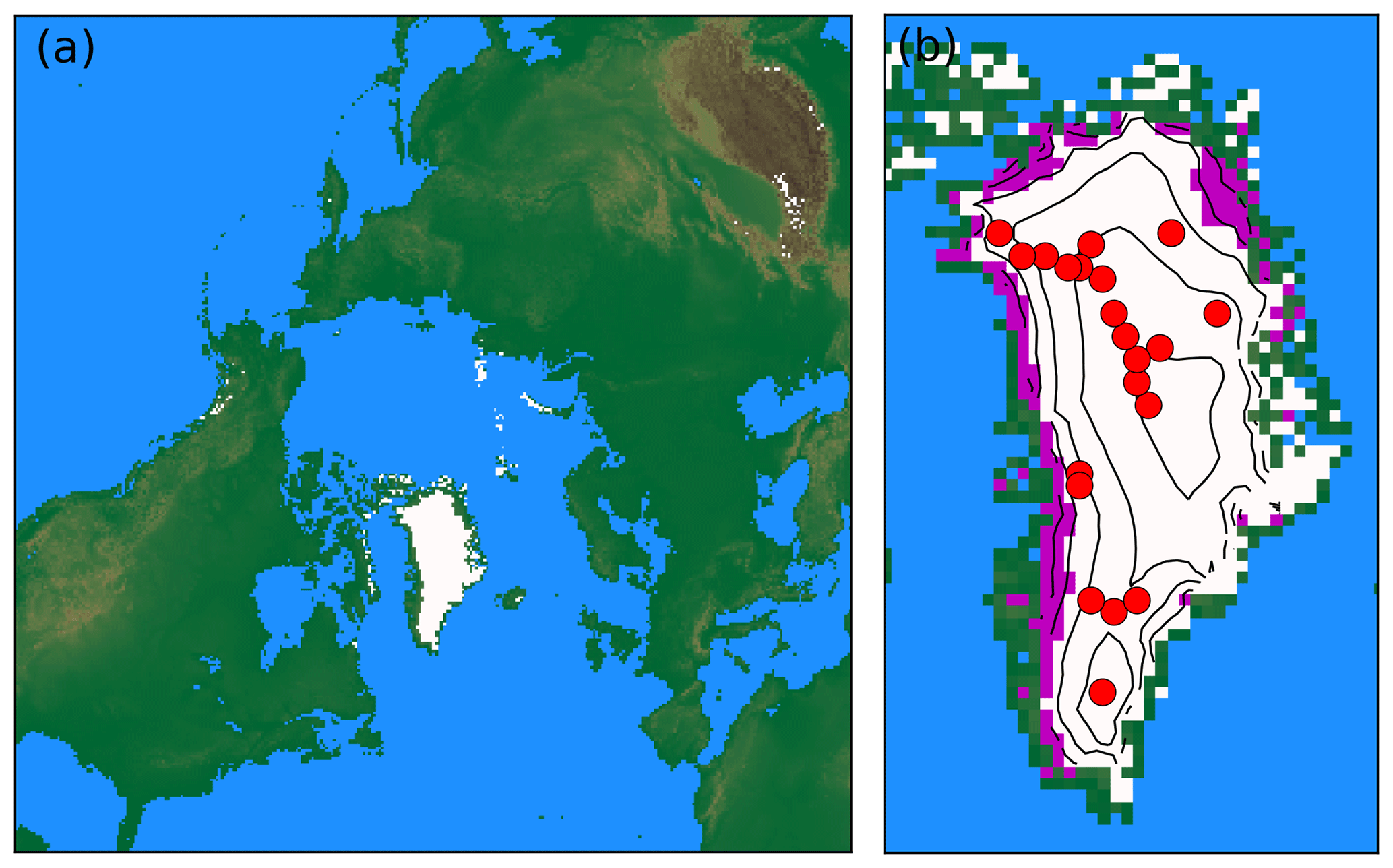
https://www.the-cryosphere.net/13/1529/2019/tc-13-1529-2019-f01

Figure 1(a) Model domain used in this study and topography based on the ETOPO1 dataset (Amante and Eakins, 2009). White areas illustrate regions with a net positive mass balance in simulation BEST_T (Sect. 3.2). (b) In addition to panel (a) magenta colours show net negative mass balance and contour lines show elevation over ice, with a spacing of 500 m. The red dots indicate locations of firn temperature measurements (Table ).

Download

https://www.the-cryosphere.net/13/1529/2019/tc-13-1529-2019-f02

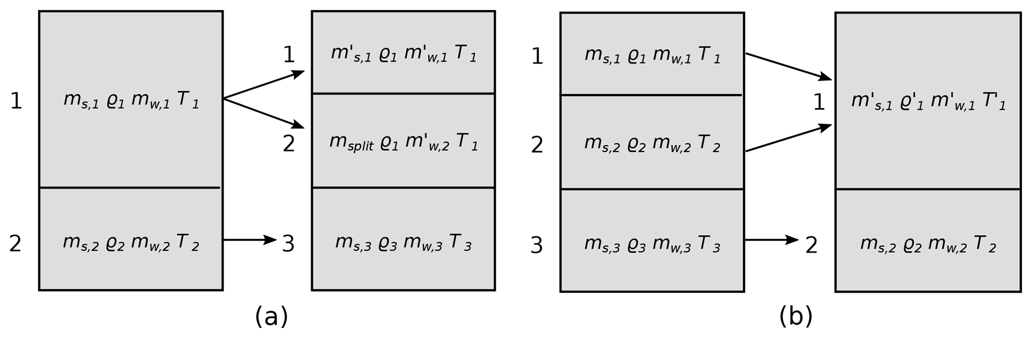
Figure 2(a) Splitting of a box that exceeds the maximum snow mass m_max. (b) Merging of two boxes in case the mass of the uppermost box falls below m_min.

Download

The vertical dimension is implemented on a mass-following dynamical grid with a given maximum number of vertical layers, n_layers. This number can in principle be chosen freely but is constant at 15 throughout this study. However, not all layers are filled at all locations at all time steps. Precipitation fills the uppermost box until it reaches the threshold value of m_max=500 kg m⁻². At this point, the box is split into two such that the lower part contains m_split=300 kg m⁻² of snow and the upper one the remaining mass. To accommodate the new subsurface grid box, the entire snow column below the former surface is shifted one grid box downward (Fig. 2a). After the split, temperature and density do not change, and the liquid water is distributed using the same ratios as for the snow mass. In case all n_layers boxes were full before the split, the two lowest boxes are merged into one.

Similarly, if the snow mass in the surface box sinks below m_min=100 kg m⁻², it is combined with the second box, if there is one (Fig. 2b). Should the combined weight be at more than twice as heavy as m_split, the mass is transferred only partially so that the surface box does not become more heavy than m_split.

Of the four variables that are simulated prognostically on the grid, snow mass m_s, liquid water m_w, density of snow ρ_s, and snow temperature T_s, liquid water is the only one that is regularly exchanged between boxes, disregarding the relatively seldom merging or splitting of boxes (Fig. 3). This simplifies the model formulation, because the advection equation does not have to be solved and it avoids spurious fluxes of heat and other tracers due to numerical diffusion. For the same reason, boxes with a depth index of 2 to 14 can only contain masses above m_split=300 kg m⁻², where liquid water refreezes. A conceptually similar vertical grid is used in the isochronal ice sheet model of Born (2017). Horizontal interactions between columns are not simulated.

https://www.the-cryosphere.net/13/1529/2019/tc-13-1529-2019-f03

Figure 3Set-up of snow layers with fluxes of energy and mass and snow quantities in one snow column.

Download

The surface box exchanges energy with the atmosphere (Q_SF) in the form of sensible, latent, and radiative heat. It receives mass as either rain (Δ m_r) or snow (Δ m_s). Temperature diffuses through the layers (Q_TD), and the snowpack densifies with time and rising overburden pressure. Meltwater and rain percolate (Δm_w) and may freeze again, which leads to internal accumulation. Water leaving the lowest grid cell is treated as run-off. Lists of all model variables and constants are found in Tables 1 and 2.

Table 1Table with all symbols used in the model.

Download Print Version | Download XLSX

Table 2Table of physical constants and model constants. The tuning parameters have their tested values listed in brackets.

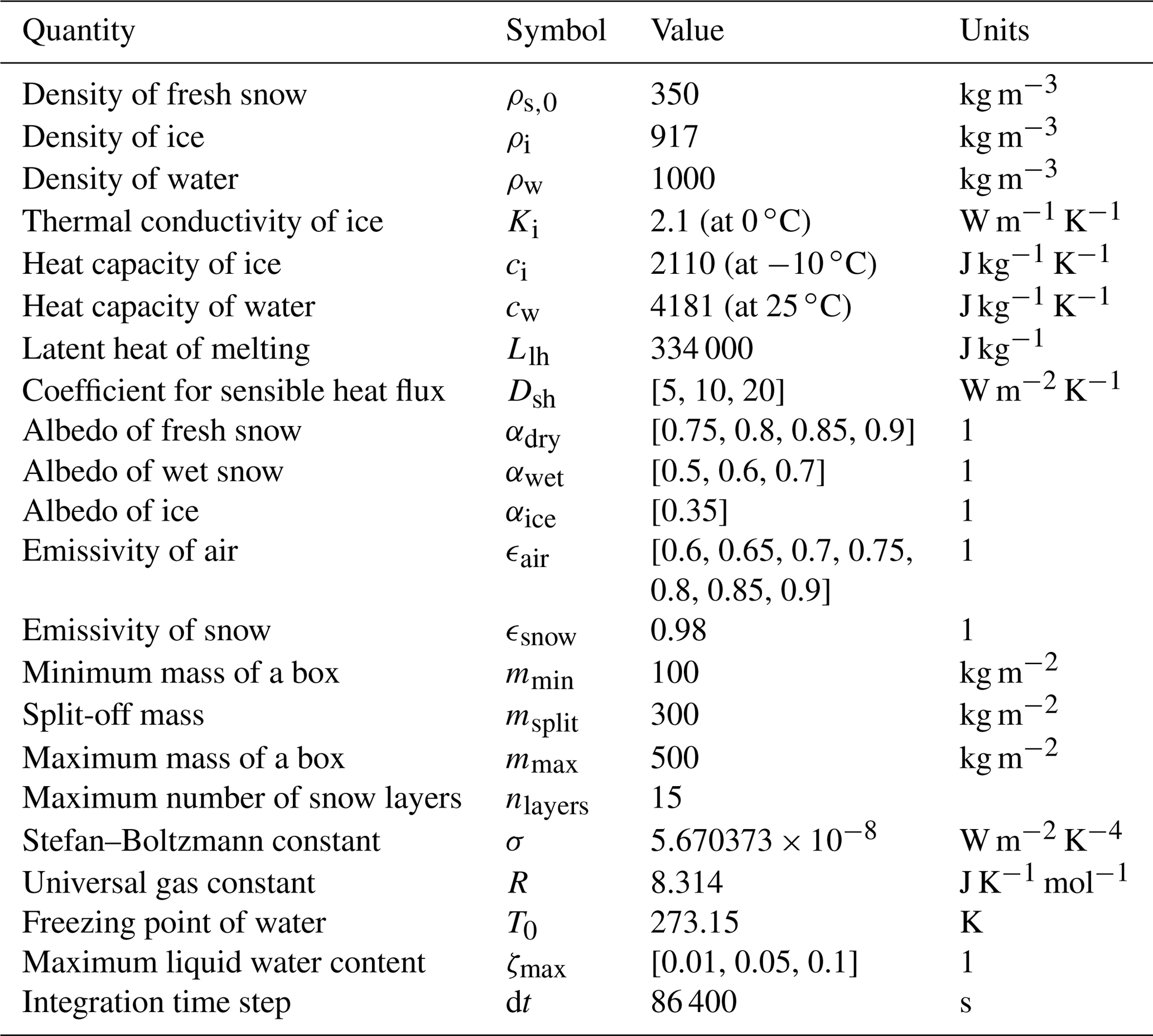
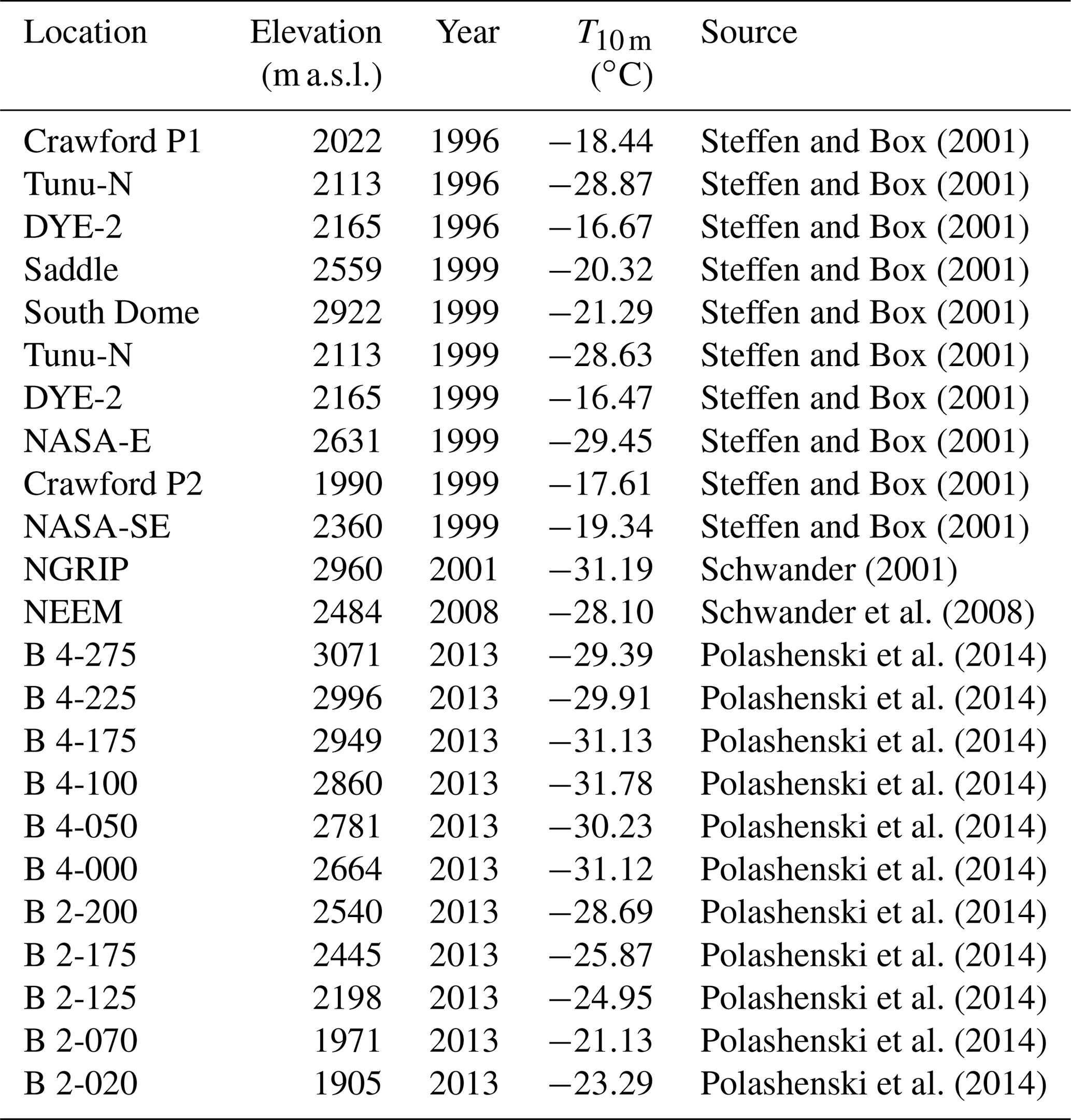
Download Print Version | Download XLSX

Table 3Measurements of annual average firn temperatures at a depth of 10 m (see map in Fig. 1).

Download Print Version | Download XLSX

2.2 Firnification

As the snow accumulates it becomes denser due to the growing overburden pressure. We follow Schwander et al. (1997) for the firnification of snow. Because the densification processes differ for densities above and below 550 kg m⁻³, two different models are used. The equations used here were calibrated for dry snow; nevertheless, we apply them to wet snow too.

Below 550 kg m⁻³, the rate of snow densification is proportional to the accumulation rate A in units kg m⁻² s⁻¹ and a temperature-dependent variable k₀ (Herron and Langway, 1980):

\begin{matrix} (1) & \frac{\partial ρ_{s}}{\partial t} = k_{0} A (ρ_{i} - ρ_{s}), \end{matrix}

where

\begin{matrix} (2) & k_{0} = 0.011 m^{2} {kg}^{- 1} \exp (\frac{- 10 160 J {mol}^{- 1}}{R \cdot T_{s}}) . \end{matrix}

By modifying the original parameterization for dry snow, here both snowfall and rain count toward the accumulation.

Densification beyond 550 kg m⁻³ follows Barnola et al. (1991). This model is more physical because it takes into account the overburden pressure and not only the implied change in pressure due to accumulation. Here, the density change is given by

\begin{matrix} (3) & \frac{\partial ρ_{s}}{\partial t} = k_{1} ρ_{s} f \cdot Δ p^{3}, \end{matrix}

where

\begin{matrix} (4) & k_{1} = 25 400 {MPa}^{- 3} s^{- 1} \exp (\frac{- 6 \cdot 10^{4} J {mol}^{- 1}}{R \cdot T_{s}}) . \end{matrix}

As k₀ above, k₁ is an empirical, temperature-dependent variable. Δp is the pressure difference between the overburden pressure and the inside gas pressure. The latter one only occurs after bubble close-off and thus is not relevant here. f is a dimensionless factor, which for densities ρ_s between 550 and 800 kg m⁻³ f is given by

\begin{matrix} (5) & \log_{10} (f) = β {(\frac{ρ_{s}}{ρ_{i}})}^{3} + γ {(\frac{ρ_{s}}{ρ_{i}})}^{2} + δ (\frac{ρ_{s}}{ρ_{i}}) + ϵ, \end{matrix}

with the empirical dimensionless parameters $β = - 29.166$ , γ=84.422, $δ = - 87.425$ , and ϵ=30.673. Finally, although this case rarely applies in the current configuration with 15 vertical layers, for densities ρ_s above 800 kg m⁻³ f is equal to

\begin{matrix} (6) & f = \frac{3}{16} (1 - (\frac{ρ_{s}}{ρ_{i}})) / {(1 - {(1 - (\frac{ρ_{s}}{ρ_{i}}))}^{1 / 3})}^{3} . \end{matrix}

2.3 Energy balance

2.3.1 Surface energy flux

The surface energy balance takes into account five different ways of exchanging energy with the atmosphere: net shortwave radiation Q_sw, thermal longwave radiation Q_lw, sensible heat exchange with the atmosphere Q_sh, heat transport by precipitation Q_p, and exchange of latent heat due to refreezing or melting of rain and meltwater Q_lh. Note that refreezing is not exclusive to the surface. The equation for the change in temperature of the surface box due to surface fluxes then reads

\begin{matrix} (7) & c_{i} m_{s, 1} \frac{\partial T_{s}}{\partial t} |_{surface} = Q_{sw} + Q_{lw} + Q_{sh} + Q_{p} + Q_{lh}, \end{matrix}

with the mass per area of the surface box m_s,1 and the heat capacity of ice c_i.

Shortwave radiation: Shortwave radiation depends only on the snow albedo (α_snow) and the incoming shortwave radiation at the bottom of the atmosphere (S_BOA), which is an input parameter provided by the climate forcing:

\begin{matrix} (8) & Q_{sw} = (1 - α_{snow}) S_{BOA} . \end{matrix}

The albedo of snow changes considerably when melting occurs and thus has an impact on how much energy of the incoming solar radiation at the bottom of the atmosphere, S_BOA, is absorbed by the surface of the snow cover. This is taken into account by using two different values for α_snow, α_dry for dry snow with temperatures below the freezing point and α_wet for wet snow with a temperature T_s=0 ^∘C. A wide range of values is plausible depending on the surface conditions: 0.7–0.98 for dry snow, 0.46–0.7 for wet snow, and for ice 0.3–0.46 (Paterson, 1999). See Table 2 for values tested.

Longwave radiation: The net longwave radiation at the snow surface is the difference between the downward directed part from the atmosphere and the upward radiation emitted by the snow:

\begin{matrix} (9) & Q_{lw} = σ (ϵ_{air} T_{air}^{4} - ϵ_{snow} T_{s}^{4}), \end{matrix}

where σ is the Stefan–Boltzmann constant, ϵ_air is the emissivity of air, and ϵ_snow is the emissivity of snow. T_air is the air temperature as provided as a boundary condition from the climate forcing. The emissivity of snow is ϵ_snow=0.98. Clouds and air humidity generally have a large impact on the net longwave radiation balance due to their high emissivity in the infrared spectrum but also the air temperature influences the emissivity of air. This is reflected in the great spread of measured values for ϵ_air. Busetto et al. (2013) suggest ϵ_air values between 0.4 and 0.7 under the very dry conditions on the Antarctic Ice Sheet, while measurements in Greenland suggest that ϵ_air takes values between 0.7 and 0.9 (Greuell, 1992; Paterson, 1999). In general, not only the near-surface air temperature is relevant for this energy flux, but also air temperatures higher up in the atmosphere. We acknowledge that one global value for ϵ_air is likely an oversimplification. However, the alternatives are using either the longwave downward radiation or the three-dimensional temperature and humidity fields and cloudiness as climate boundary conditions, which are not readily available from coarse-resolution climate model that BESSI is designed to be coupled with.

Sensible heat flux: The bulk coefficient for the sensible heat flux D_sh is (Braithwaite, 2009):

\begin{matrix} (10) & D_{sh} = 1.29 \times 10^{- 2} K^{- 1} \cdot A p u, \end{matrix}

where u is the wind speed, p the average atmospheric pressure, and A and empirical, dimensionless transfer coefficient. A takes values between 1.4 and $3.6 \times 10^{- 3}$ . Assuming an air pressure of p of 10⁵ Pa and a wind speed of 5 m s⁻¹, D_sh takes values between 9 and 23 W m⁻² K⁻¹. The net sensible heat flux is given by the following:

\begin{matrix} (11) & Q_{sh} = D_{sh} (T_{air} - T_{s}) . \end{matrix}

Heat transport with precipitation: Snow and rain falling onto the snow generally do not have the same temperature as the firn and thus represent a heat sink or source.

\begin{array}{l} (12) & Q_{p, rain} = P \cdot ρ_{w} c_{w} (T_{air} - T_{0}), \\ (13) & Q_{p, snow} = P \cdot ρ_{w} c_{i} (T_{air} - T_{s}), \end{array}

where P is the precipitation and ρ_w the density of water. c_w and c_i are the heat capacities of water and ice. T₀ is the freezing temperature of water at sea level. This sensible heat of the precipitation only influences the surface box of the snow column. The latent heat due to freezing and melting may affect deeper layers as well and is therefore treated separately and described below.

Latent heat flux: The heat released by the melting of snow or freezing of water is as follows:

\begin{array}{l} (14) & Q_{lh, melt} = - L_{lh} \cdot m_{s}, \\ (15) & Q_{lh, refreeze} = L_{lh} \cdot m_{w}, \end{array}

where L_lh is the specific heat of fusion. While melting may only occur at the surface, freezing of liquid water is allowed to take place everywhere in the snow column.

2.3.2 Diffusion of heat

Below the surface, heat is transported by diffusion and as latent heat in liquid water. Temperature differences between the vertical layers cause diffusion of heat:

\begin{matrix} (16) & c_{i} ρ_{s} \frac{\partial T_{s}}{\partial t} = \frac{\partial}{\partial z} (K (ρ_{s}) \frac{\partial T_{s}}{\partial z}), \end{matrix}

where K(ρ_s) is the thermal conductivity of snow as a function of the density of snow (Yen, 1981):

\begin{matrix} (17) & K (ρ_{s}) = K_{i} {(\frac{ρ_{s}}{ρ_{w}})}^{1.88} . \end{matrix}

However, this approximation does not account for the effects of liquid water or the influence of the snow structure.

2.4 Mass balance

2.4.1 Surface accumulation and ablation

Accumulation: Depending on the air temperature at each time step, either snow or rain falls on the top grid cell. Generally all precipitation that falls below the freezing point of water is considered to be snow with a temperature equal to that of the air. Snowfall is directly added to the mass of the first grid box as

\begin{matrix} (18) & \frac{\partial m_{s, 1}}{\partial t} = P \cdot ρ_{w} . \end{matrix}

Precipitation at time steps with an air temperature above 0 ^∘C is treated as rain with air temperature and is added to the water content of the surface box:

\begin{matrix} (19) & \frac{\partial m_{w, 1}}{\partial t} = P \cdot ρ_{w} . \end{matrix}

The temperature difference between rain and the freezing point causes an energy flux into the snow cover as detailed in Sect. 2.3.1. All water in the pore volume of the snow has an assumed temperature of 0 ^∘C. Sublimation and windborne redistribution of snow are not included. While they are usually negligible in regions of relatively high accumulation, sublimation in central Greenland is estimated to be 12 %–23 % of the precipitation under present-day conditions (Box and Steffen, 2001).

Ablation: If the net incoming energy at the surface warms the surface layer to temperatures above the melting point, the temperature is kept at 0 ^∘C and the excess heat is used to melt snow (Eq. 14). Should the top layer melt entirely, the remaining energy is used to heat the next layer to 0 ^∘C and then melt it. This process is repeated until the entire melt energy is consumed. The resulting meltwater is added to the liquid water mass m_w of the corresponding layers. In the case that the entire snow column melts, the remaining energy is used to melt ice. Bare ice is also assumed to be at 0 ^∘C. Water from melted ice is treated as run-off and removed from the model immediately.

2.4.2 Percolation and refreezing of water

Percolation: Water may fill the pore volume in the snow up to a certain maximum fraction ζ_max (Greuell, 1992). Water in excess of this maximum percolates downwards to the next box where the same fraction applies. Water that leaves the lowest active box is deemed to be run-off and removed from the model. The fractional liquid water content of a grid cell is calculated as follows:

\begin{matrix} (20) & ζ = \frac{m_{w}}{m_{s}} \frac{1}{ρ_{w} \cdot (\frac{1}{ρ_{s}} - \frac{1}{ρ_{i}})} . \end{matrix}

For snow densities close to that of ice ρ_i, numerical problems arise due to division by (almost) zero. Thus, all water percolates downwards if the grid cells density satisfies $ρ_{s} > ρ_{i} - 10$ kg m⁻³. This happens in areas with a lot of rain and meltwater that freezes again during the winter. Measurements at the ETH camp in Greenland suggest a value of 0.1 for ζ_max, but lower values are also used (Greuell, 1992).

Refreezing: If water percolates into colder layers or when temperatures decrease, it may freeze again, leading to internal accumulation. Since the time steps are relatively long and the pores in the firn are rather small, we assume that the liquid water is in thermodynamic equilibrium with the surrounding snow. If the snow is not cold enough, it is possible that water freezes only partly. In this case the snow is heated to 0 ^∘C and the energy $(T_{0} - T_{s}) \cdot c_{i} \cdot m_{s}$ is used to freeze the corresponding amount of water (Eq. 15). If all water freezes and the snow has now the following temperature

\begin{matrix} (21) & T_{s}^{'} = \frac{m_{w} \cdot L_{lh} / c_{i} + T_{0} \cdot m_{w} + T_{s} \cdot m_{s}}{m_{w} + m_{s}} . \end{matrix}

In both cases, snow density ρ_s, mass m_s, and the mass of water m_w are adjusted accordingly, conserving the volume of the grid box.

2.4.3 Surface mass balance for the ice model

If the total mass of the entire snow column exceeds $m_{column} = 1.5 \cdot m_{split} \cdot n_{layers}$ at the end of the year, the surplus mass is removed from the bottom and transferred to the ice model. The factor of 1.5 is applied so that snow is rarely removed from the second lowest layer and only in snow columns where significant amounts of refreezing occurs. In perennially cold areas the lowest grid box grows very thick. Transferring the surplus accumulation from each snow column results in an even field of accumulation being passed on to the ice model, in contrast to passing full boxes whenever they reach a certain threshold. This avoids numerical instabilities in the ice dynamics code.

2.5 Climate input data

BESSI only requires precipitation, shortwave radiation at the bottom of the atmosphere, and surface air temperature as boundary conditions. With the exception of Sect. 5, these fields are taken from the ERA-Interim climate reanalysis (Dee et al., 2011). The forcing consists of daily averages for 38 years, from 1979 to 2016. Since the climate forcing data are not referenced to the same topography as the one in BESSI, the temperature field is corrected with a constant lapse rate of 0.0065 K m⁻¹. Shortwave radiation and precipitation are not corrected, although changes in elevation modify the optical depth of the atmosphere and the transport of moisture. The temporal resolution of the input data is 365 time steps per year. The model has also been tested with a longer time step of 96 per year, which corresponds to the time step of the Bern3D coarse-resolution climate model (Ritz et al., 2011). The longer time step produces good results, but they have not been tested thoroughly and are therefore not included here.

2.6 Numerical implementation

BESSI is implemented in FORTRAN90 as a subroutine of the ice sheet model IceBern2D (Neff et al., 2016). The decision tree and calculation flow at each time step is shown in Fig. 4. The model iterates through all grid cells on land with a time step of 1 day. At every time step, calculations are executed for every active snow layer if not specified otherwise.

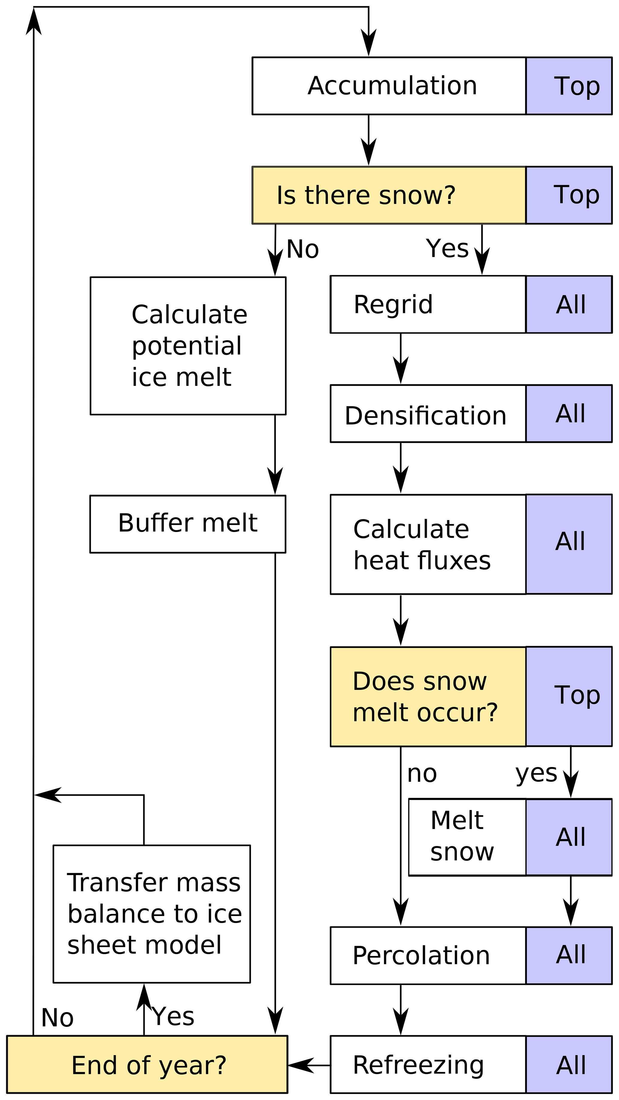
https://www.the-cryosphere.net/13/1529/2019/tc-13-1529-2019-f04

Figure 4Decision tree at each time step. The blue boxes denote whether the process or question concerns only the top layer or all layers.

Download

The first step during every iteration is accumulation at the surface. Depending on the air temperature either snow or rain is accumulated and added to the corresponding mass variable of the surface box (Sect. 2.4.1). The accompanying heat transport is stored as an energy flux which will be used later during the time step along with all other energy fluxes. At grid boxes where there is no snow present after this step, the potential melt of ice is calculated with the energy that enters a hypothetical ice layer during that time step. In these grid boxes, the time step ends here.

Where there is snow present, the layers are regridded if necessary (Sect. 2.1), and the densification is calculated (Sect. 2.2). In order to save calculation time, only columns with three and more layers of snow are densified. Most cells that only carry seasonal snow do not need more than two active snow boxes, and densification is negligible where the snow disappears completely every year.

The surface energy balance and diffusion within the snow (Eqs. 7 and 16) are solved in a single step using an implicit leapfrog scheme. However, this may heat the snow to temperatures above 0 ^∘C. When this happens, the result is discarded and the calculation is repeated without surface heat flux but with a fixed surface snow temperature of 0 ^∘C. The energy necessary to heat the surface box to the melting point is subtracted from the available melting energy to ensure energy conservation. Melting only occurs at the surface and the corresponding amount is added to the water mass of the uppermost box. However, if the surface layer melts completely, the mass-following grid is adjusted accordingly so that more than one snow layer may melt in one time step.

Now, the percolation of the liquid water in the snow layers is calculated. This includes both meltwater and rain. The routine starts at the top box and works down through all active boxes. Water only travels downwards and at the end of this step no grid box contains more water than the fraction ζ_max of the pore volume (Sect. 2.4.2). Some of the percolated water may refreeze in the snow. This process can accelerate the densification process of the firn and it modifies the heat profile.

Finally, excess mass is removed from the bottom of the snow column at the end of each model year and combined with the accumulated potential melt from the beginning of all time steps to calculate the mass balance for the ice model. The integrated balance is transferred to the ice model. From here on the procedure is repeated with the input parameters from the next time step.

3 Model assessment and calibration

3.1 Conservation of mass and heat

In order to verify energy and mass conservation in BESSI, all mass and energy fluxes into and out of the snow cover are summed up separately (diagnosed) and compared with the effective changes in snow mass and snow energy content simulated by the model. This is done in a simulation that is forced with climatological daily averages created from the 1979–2016 ERA-Interim climatology. The snow model is well equilibrated after 5000 model years. There are $15 \cdot 313 \cdot 313 \approx 1.5 \times 10^{6}$ grid cells on the model domain, each being calculated at FORTRAN double precision of 10⁻¹⁶. Thus the maximum relative error of total mass and energy fluxes on the entire domain with 64 bit machine precision should not be larger than $1.5 \times 10^{6} \cdot 10^{- 16} \approx 10^{- 10}$ .

https://www.the-cryosphere.net/13/1529/2019/tc-13-1529-2019-f05

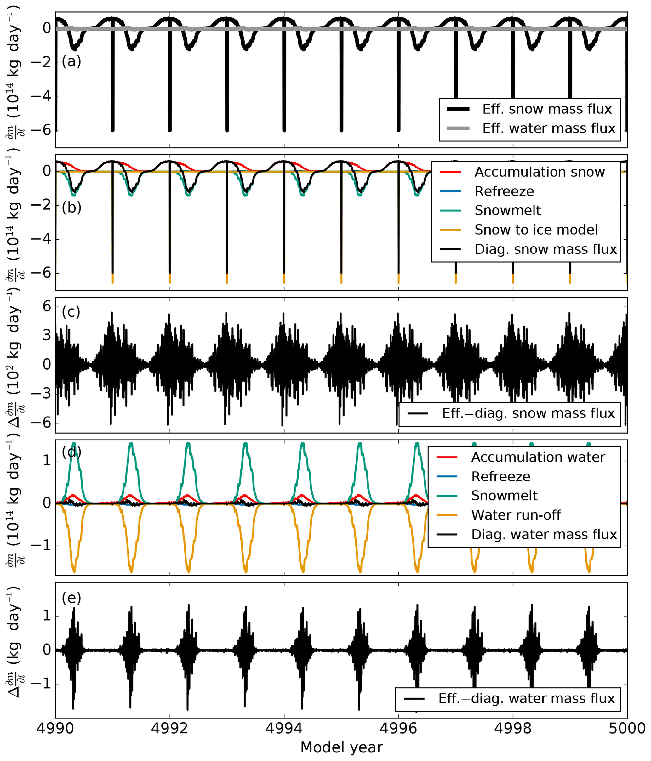
Figure 5Total mass fluxes summed up over the entire model domain 5000 years after initialization. (a) Effective changes in snow and water mass inside the snow model. (b) Diagnosed fluxes in snow mass with all its contributing terms. (c) Effective minus diagnosed snow mass fluxes. (d) Diagnosed fluxes in water mass with all its contributing terms. (e) Effective minus diagnosed water mass fluxes.

Download

Conservation of mass: Mass is added to the snow cover as snow and rain. The model loses mass by percolation of water out of the lowest active box or by passing mass to the ice model. The comparison of effective changes in the amount of snow and water in the model domain and the sum of the components of mass fluxes show that the relative error is largest during winter and spring when the snow mass is at its maximum but never above 10⁻¹² (Fig. 5). Over the 5000-year simulation time, the average unaccounted mass flux for the entire model domain is −2.09 kg a⁻¹. For liquid water, the relative error is less than 10⁻¹³ with an average loss of −1.23 kg a⁻¹ for the entire domain. Thus, we conclude that the model conserves mass within computational accuracy.

Conservation of energy: The energy fluxes into and out of the snow model comprise surface energy fluxes and latent heat of snow and rain, by snow and water that leave the model at the lower boundary. Internal fluxes such as the thermal diffusion and the redistribution of latent heat by the liquid water must not change the energy content.

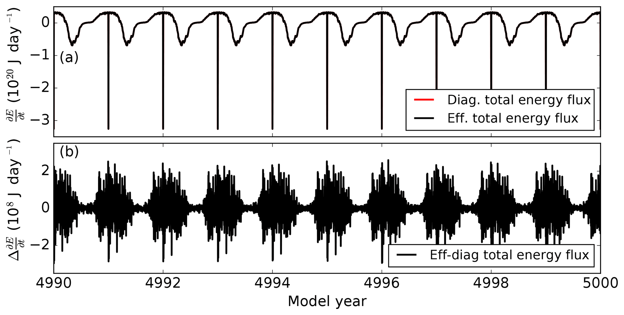
https://www.the-cryosphere.net/13/1529/2019/tc-13-1529-2019-f06

Figure 6Total energy fluxes integrated over the entire model domain after 5000 model years. (a) Diagnosed and effective total energy flux, the former being covered by the latter. (b) Observed minus diagnosed total energy flux. Abrupt changes in the time series are due to energy (and mass) transfer to the ice sheet model (compare Fig. 5b).

Download

Indeed, the relative error between the observed changes in heat content and the sum of the fluxes at the upper and lower boundaries is 10⁻¹² and thus also conserved to machine precision (Fig. 6). The average loss of heat is −167 917.7 J a⁻¹, equivalent to melting of about 0.5 kg of ice.

3.2 Model calibration

To reduce the parametric uncertainty of BESSI, a large ensemble of simulations is carried out based on the five most uncertain parameters. The calibration uses observations of the annual mean 10 m firn temperature from Greenland, annual cumulative Greenland mass loss data, and the monthly extent of the snow cover of the entire model domain. This selection is made to assess both the energy and mass balance of the model, for both perennially and seasonally snow-covered regions.

To calibrate the flux of heat we compare the model results with 23 firn temperature measurements from Greenland that were taken between 1996 and 2013 (Table ). A similar approach was taken by Steger et al. (2017) with the measurements of Polashenski et al. (2014). Here we extend this data set with firn temperature measurements from Steffen and Box (2001), Schwander (2001), and Schwander et al. (2008) to achieve a broader spatial and temporal coverage of the Greenland ice sheet. The 10 m firn temperature measurements of Steffen and Box (2001) are part of the Greenland Climate Network (GC-Net) and not maintained regularly, thus leading to poor control over the depth of the firn temperature sensors. Therefore, only a selection of measurements is used that were taken less than 3 years after activation of the measurement site. Two additional measurements were included from the North Greenland Ice Core Project (NGRIP) and the North Greenland Eemian Ice Drilling (NEEM) sites (Schwander, 2001; Schwander et al., 2008). Although these were taken in summer, they are interpreted to be representative of the annual average because the 10 m temperatures of GC-Net vary by less than 0.5 ^∘C over the annual cycle.

The seasonal snow cover is compared with satellite data from January 1979 to December 2016 (Northern Hemisphere EASE-Grid 2.0 Weekly Snow Cover and Sea Ice Extent, Version 4; Brodzik and Armstrong, 2013). The weekly data are downsampled to a monthly resolution and interpolated onto the grid of BESSI. In the model, a grid cell is counted as covered with snow when the snow mass per area m_s is more than 25 kg m⁻², about 1 cm of fresh snow.

Changes in the total mass of the Greenland ice sheet are compared with measurements from the Gravity Recovery and Climate Experiment (GRACE; Watkins et al., 2015; Wiese et al., 2016). Observed changes in surface mass balance are calculated by subtracting the estimated increase in calving since 1996 (van den Broeke et al., 2016). We used cumulative annual averages for the years 2002 to 2018.

The five model parameters that are chosen to define the ensemble are the bulk coefficient for sensible heat flux D_sh, the albedo of dry snow α_dry, the albedo of wet snow α_wet, the air emissivity ϵ_air and the maximum water content ratio of the pore volume ζ_max. Each parameter is perturbed within its realistic range (Table 2) for a total of 756 simulations.

All simulations are forced with daily average data from the ERA-Interim climate reanalysis for the period 1979–2016 (Sect. 2.5). For each parameter combination BESSI is initialized with snow by applying the climatic forcing of the years 1979–1998 forward and backward 6 times. The last 18 years are not used for the initialization because of their warming trend. The aim of the initialization sequence is to attain a firn that most closely resembles conditions at the beginning of the year 1979. After these 240 years of initialization BESSI is fully equilibrated in the sense that all snow columns with a positive mass balance are filled with snow and forward mass to the ice sheet domain of the model. Subsequently, the years from 1979 to 2016 are simulated.

The quality of all simulations is quantified by calculating the root-mean-square error (RMSE) of the modelled data:

\begin{matrix} (22) & {RMSE}_{X} = \sqrt{\frac{1}{i} \sum_{x = 1}^{i} {(X_{model, i} - X_{obs, i})}^{2}}, \end{matrix}

where i is the number of observations, and $X_{model, i} - X_{obs, i}$ is the difference between simulated and observed data. The number of observations i corresponds to the number of borehole sites (RMSE_T, 23), the years of mass loss measurements (RMSE_m, 16), and the total number of grid points in the domain multiplied by the number of months in the observational record for the snow cover observations (RMSE_A, 43 498 236).

https://www.the-cryosphere.net/13/1529/2019/tc-13-1529-2019-f07

Figure 7RMSE for monthly snow area A (top row), Greenland borehole temperature T (middle row; note the broken vertical scale), and Greenland mass balance m (bottom row), for five model parameters. Dark grey ranges contain 50 % of the ensemble simulations; light grey is 90 %. The horizontal black line shows the median.

Download

Table 4 lists the parameter values that lead to the best agreement with observations, i.e. the average values of the 10 simulations with lowest RMSE. The ideal parameters for all three metrics are reasonably close, with the exception of the bulk transfer coefficient for sensible heat D_sh. Additional detail can be found in the distributions of RMSE for single parameters (Fig. 7). The atmospheric emissivity ϵ_air has a pronounced effect on the width and the median of the distributions, with a clear minimum within the range of tested values. This minimum is at lower values for the firn temperature than for the extent of the seasonal snow cover or the Greenland mass balance, probably because the firn temperatures have a regional bias to high-altitude regions on Greenland where relatively dry and thin air reduce the downward flux of longwave radiation.

Table 4Parameter combinations averaged over the 10 simulations with lowest RMSE for monthly snow area TOP_A, Greenland borehole temperature TOP_T, and Greenland mass balance TOP_m, and the single simulation with the lowest RMSE for each metric (BEST_X).

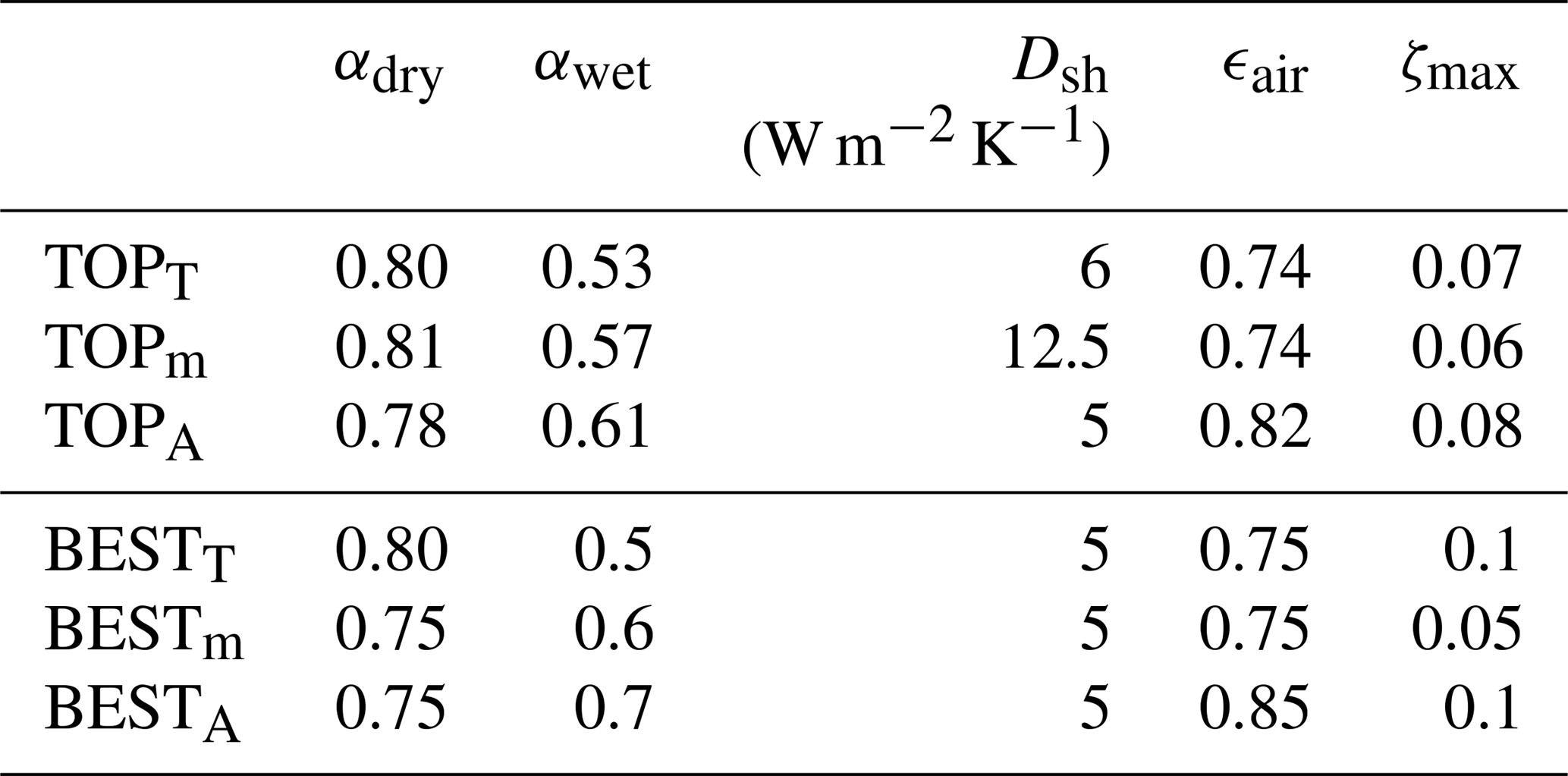
Download Print Version | Download XLSX

D_sh does not have a clear optimum value within the range of tested values. This indicates that higher values are possible, perhaps due to wind speeds that exceed the 5 m s⁻¹ that were postulated for the estimate of D_sh above. The reduction in the spread for higher values of D_sh suggests that other forms of heat exchange with the atmosphere become comparably less relevant.

4 Comparison with observations

In this section we analyse one simulation in more detail and compare it to some key observations. The simulation chosen is the one with the lowest RMSE for the borehole temperature, BEST_T, unless explicitly specified otherwise (Table 4). Regions of net positive mass balance in BESSI compare well to glaciated areas, including ice caps in the Canadian and Russian Arctic, southeast Iceland, southeast Alaska, Svalbard, and the Pamir and Karakoram ranges (Fig. 1). Regions where the glaciation is below the grid size of the model are not reproduced, such as the European Alps, the Caucasus Mountains and the coastal parts of Scandinavia.

BESSI simulates the seasonal snow cover with adequate accuracy, including intermittent snow events such as the one that covered central Europe in mid-December 2012 (Fig. 8). During the melting season, large parts of the snow contain liquid water. On Greenland, liquid water starts to appear at the margins in early summer (Fig. 8b) and gradually moves to higher elevations. At the beginning of the cold season, water that is close to the surface freezes again, but above 2000 m elevation this process is slower due to the thermal insulation of the relatively thick firn which leads to two banded regions of liquid water, most notably in west Greenland (Fig. 8c). In some regions the water never freezes so that water is present even at the end of the cold season (Fig. 8a). This mechanism and the region in which it occurs are captured realistically by BESSI when compared to more sophisticated models and observations (Forster et al., 2014). However, BESSI probably underestimates the extent of the so-called perennial firn aquifer, because it only simulates the upper 15 m of the firn column.

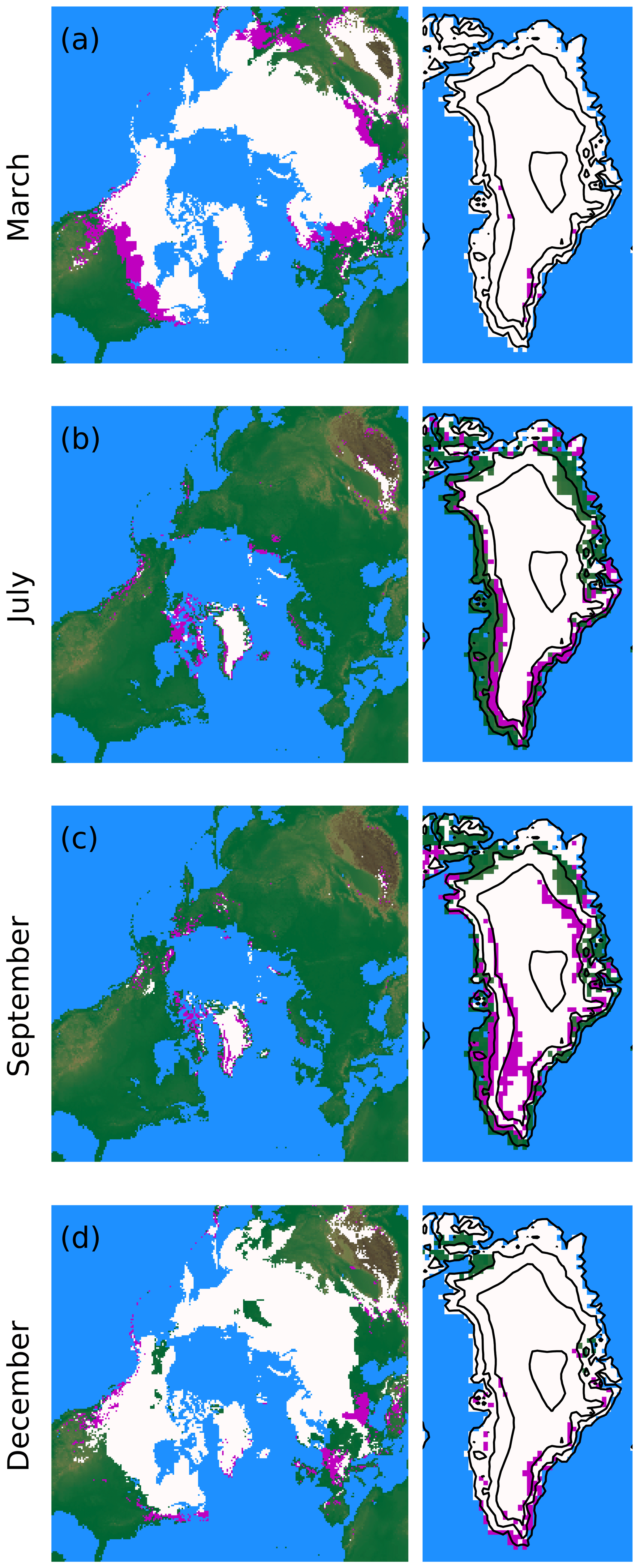
https://www.the-cryosphere.net/13/1529/2019/tc-13-1529-2019-f08

Figure 8Seasonal snow extent for the year 2012, simulation BEST_T. White areas contained at least 25 kg m⁻¹ snow at the middle of the respective month. Magenta highlights the presence of liquid water at any depth in the firn column. Contour levels show elevation with a spacing of 1000 m in the right column. Meltwater in the firn does not freeze immediately at the beginning of the winter season, which leads to the two bands of liquid water in west Greenland in September. Some regions never freeze all meltwater so that liquid water is present year round.

Download

https://www.the-cryosphere.net/13/1529/2019/tc-13-1529-2019-f09

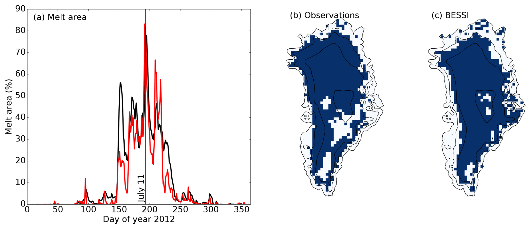
Figure 9Melt extent of the year 2012, simulation BEST_T. (a) Fractional melt area from observations (red) and BESSI (black), (b) observed melt area on 11 July, (c) same as panel (a) for BESSI.

Download

Although the model is designed for efficiency and simulations over multiple millennia, short-term events are represented with reasonable accuracy as well. Most of the surface of the Greenland ice sheet experienced melting during the extreme melt season of 2012. BESSI cannot directly capture these melt events of relatively short duration, because its surface grid box is about 1 m thick and layers of melt are typically only a few centimetres thick. To accommodate this fact but nevertheless be able to qualitatively compare our simulation with observations, we define a melt day as the surface temperature in the model exceeding −5 ^∘C. Using this metric, BESSI agrees well with microwave radiometry observations (Fig. 9) (Mote, 2014).

The firnification process also compares well with the few available observations (Fig. 10). The version used here is limited to 15 vertical layers for efficiency and so only represents the approximately linear increase in firn density. However, a version of BESSI with an extended bottom also captures the curvature in the depth-density profile at around 550 kg m⁻³ (not shown). The mismatch of the density at the surface is due to the density of the newly accumulated snow, which is fixed in the model.

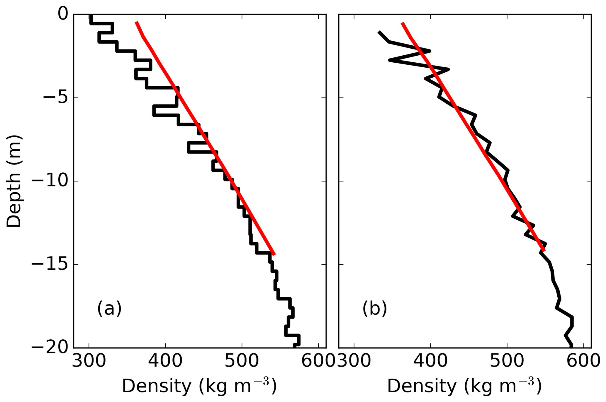
https://www.the-cryosphere.net/13/1529/2019/tc-13-1529-2019-f10

Figure 10Modelled firn densities (BEST_T) at NGRIP (a) and NEEM (b) in red. Firn measurements of Schwander (2001) and Schwander et al. (2008) in black.

Download

https://www.the-cryosphere.net/13/1529/2019/tc-13-1529-2019-f11

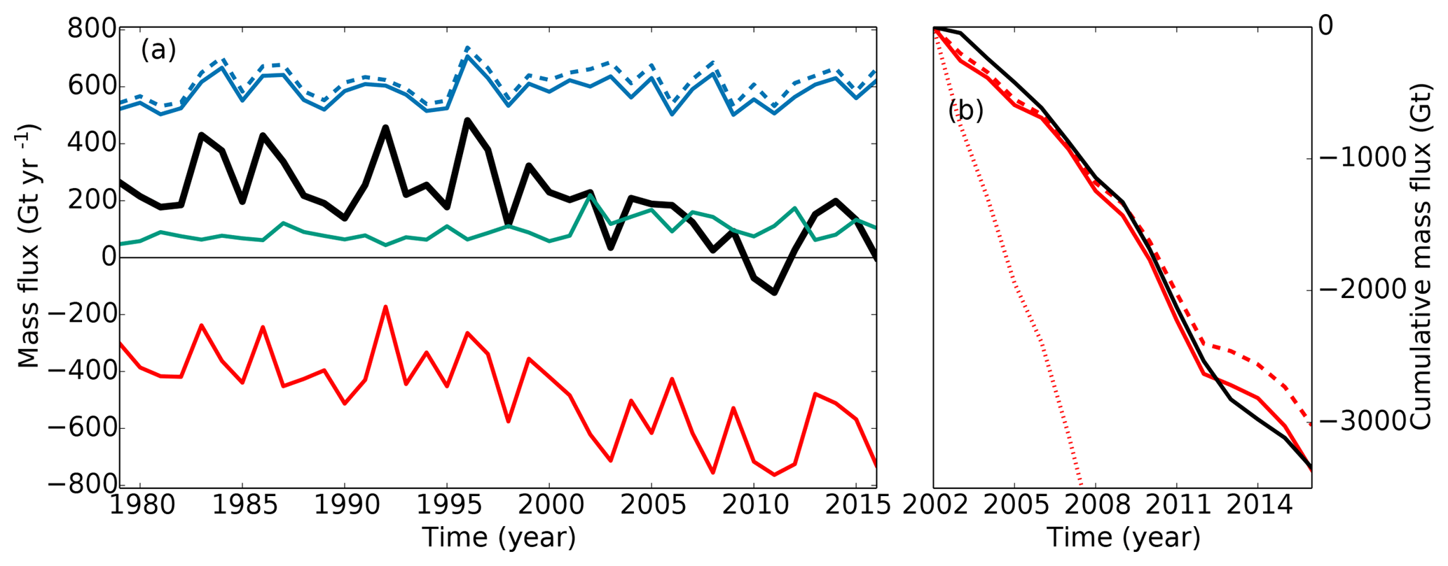
Figure 11Surface mass balance as simulated by BEST_m. (a) Total surface mass balance (black) and its components: accumulation (blue), total precipitation (blue dashed), melting (red), and refreezing (green). (b) Cumulative annual mass balance for GRACE (black), BEST_m (red), BEST_T (red dashed), and BEST_A (red dotted).

Download

Comparison of the simulated surface mass balance with more complex models reveals both good agreement as well as shortcomings (Fig. 11a). Here, we show results from the simulation BEST_m, which best reproduces the calving-corrected estimate of cumulative mass changes from GRACE (Fig. 11b). Surface melting increased from 400 Gt yr⁻¹ in 1990 to 700 Gt yr⁻¹ in 2015, while accumulation remained largely stable and refreezing increased slightly. These results and interannual variations are in good agreement with the comprehensive regional atmosphere and snow surface model RACMO2.3 (van den Broeke et al., 2016). However, while the absolute values for the total surface mass balance and the amount of melting are accurate, the total surface mass balance is 200 Gt yr⁻¹ below that of the comprehensive model. We attribute this to two factors, the lower total precipitation in the ERA-Interim dataset than in RACMO2.3, which accounts for approximately 100 Gt yr⁻¹ of the difference, and because BESSI greatly underestimates the amount of refreezing, an additional 100–150 Gt yr⁻¹ difference. A similar conclusion is drawn from the comparison of surface mass balance fields with the regional climate model MAR where the difference is especially notable for warm climate anomalies (Plach et al., 2018, Figs. 7 and 12). This result and the clear latitudinal bias of BESSI suggest that this mismatch in refreezing is due to the missing representation of the diurnal melt–freeze cycle, that was found to have a strong latitudinal pattern due to the solar elevation angle (Krebs-Kanzow et al., 2018). It is worth noting that BESSI simulates a much more positive surface mass balance with different parameter combinations, at the cost of a reduced agreement with the cumulative mass balance.

In spite of the mismatch of the total mass balance, the regional structure is captured well in comparison with RACMO2.3 (Fig. 12). The highest values of net accumulation are found in the southeast with gradually lower accumulation toward the north due to less precipitation. Net mass loss is concentrated on the western and northeastern margins, where melting extends far into the interior of the ice sheet. The narrow ablation zone in the southeast is not well reproduced because of the coarse grid. In response to the warming in recent years, the mass balance strongly decreased around the margins and slightly increased in the interior. The decrease is the result of a strongly increased melting and lower refreezing at relatively low elevations where the snow was at its water-holding capacity and refreezing potential already before the warming. As seen before, refreezing increases somewhat in recent years but not to the extent that is simulated by RACMO2.3. The regional distribution of refreezing is in good agreement with the more complex model.

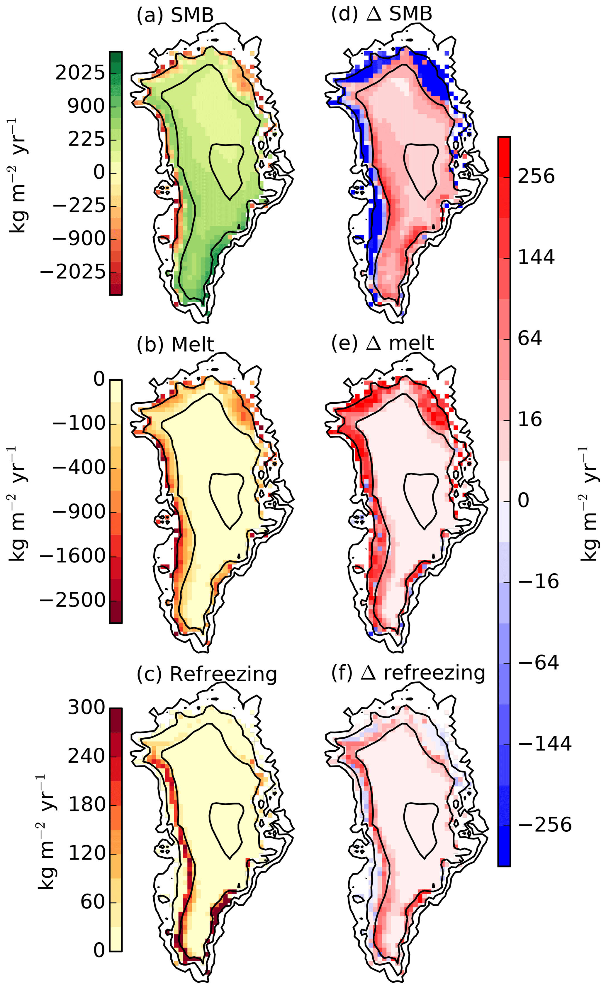
https://www.the-cryosphere.net/13/1529/2019/tc-13-1529-2019-f12

Figure 12Surface mass balance as simulated by BEST_m. Panels (a), (b), and (c) show the 1979–1990 average, panels (d), (e), (f) the difference 1991–2016 minus 1979–1990. Note the non-linear colour scales.

Download

Simulation BEST_T also shows a good agreement with GRACE in spite of being tuned to the Greenland borehole temperatures. Lastly, simulation BEST_A fails this test with a much too negative mass balance. The comparison of the model parameters (Table 4) shows that the main difference between the three simulations is the value of ϵ_air, which is 0.75 for the simulations optimized for the Arctic climate of Greenland (BEST_m, BEST_T) and 0.85 for BEST_A. The latter is sensitive to the extent of the seasonal snow cover, which mostly depends on the midlatitudes, where the atmosphere contains more moisture and clouds. The distribution of RMSE_A clearly shows a minimum at higher values of ϵ_air than for RMSE_T or RMSE_m (Fig. 7).

5 Non-linearity of the surface mass balance

It is generally accepted that the mass balance–temperature relationship has a negative curvature, meaning that positive temperature anomalies result in a stronger reduction of the mass balance than a corresponding temperature anomaly of the opposite sign would increase the mass balance (Fettweis et al., 2008; Mikkelsen et al., 2018). However, a higher air temperature also increases its capacity to hold and transport moisture, resulting in higher precipitation rates that may increase accumulation and thus counteract the more intense melting.

The numerical efficiency of BESSI allows for relatively fast calculations of large ensembles. Here we take advantage of this feature to quantify the reproduction of the non-linear characteristics of the surface mass balance. BESSI is initialized in the same way as before, where the forcing with the ERA-Interim climate reanalysis data from 1979 to 1998 is run 6 times forward and backward. After that, the model is run for the years 1979 to 1999, where a climate anomaly is added to the final year. This anomaly is defined by the annual average temperature difference over Greenland of a given year in a simulation of the Community Earth System Model version 1 (CESM1) with respect to the reference period 1950–1979 in the same simulation. The CESM1 simulation ran with full historic forcing from the year 850 to 2100 (Lehner et al., 2015), from which we use every fifth year between 1400 and 1995 here, and every year from 2000, to achieve a relatively even coverage of the temperature anomaly range. The simulations with BESSI may either use both the temperature and precipitation anomalies (ΔT and ΔP) or the temperature anomalies alone (ΔT only), which results in a total of 442 simulations with a temperature anomaly range from −5 to +7.5^∘. In addition, we also run 17 simulations with spatially uniform temperature anomalies from −8 to +8^∘. The shortwave radiation is unperturbed and all simulations in this ensemble use the BEST_T parameter settings.

As expected, the surface mass balance becomes increasingly negative for higher temperatures in the absence of accompanying factors, creating a curve with negative curvature (Fig. 13, green). Although more complex in their spatial structure, the same finding applies to temperature anomalies derived from CESM1 (red). Finally, if both temperature and the corresponding precipitation anomalies are applied, the picture is less clear, as the points on the ΔT–ΔSMB plane are more dispersed. The curvature remains negative but the SMB may increase for small perturbations (black).

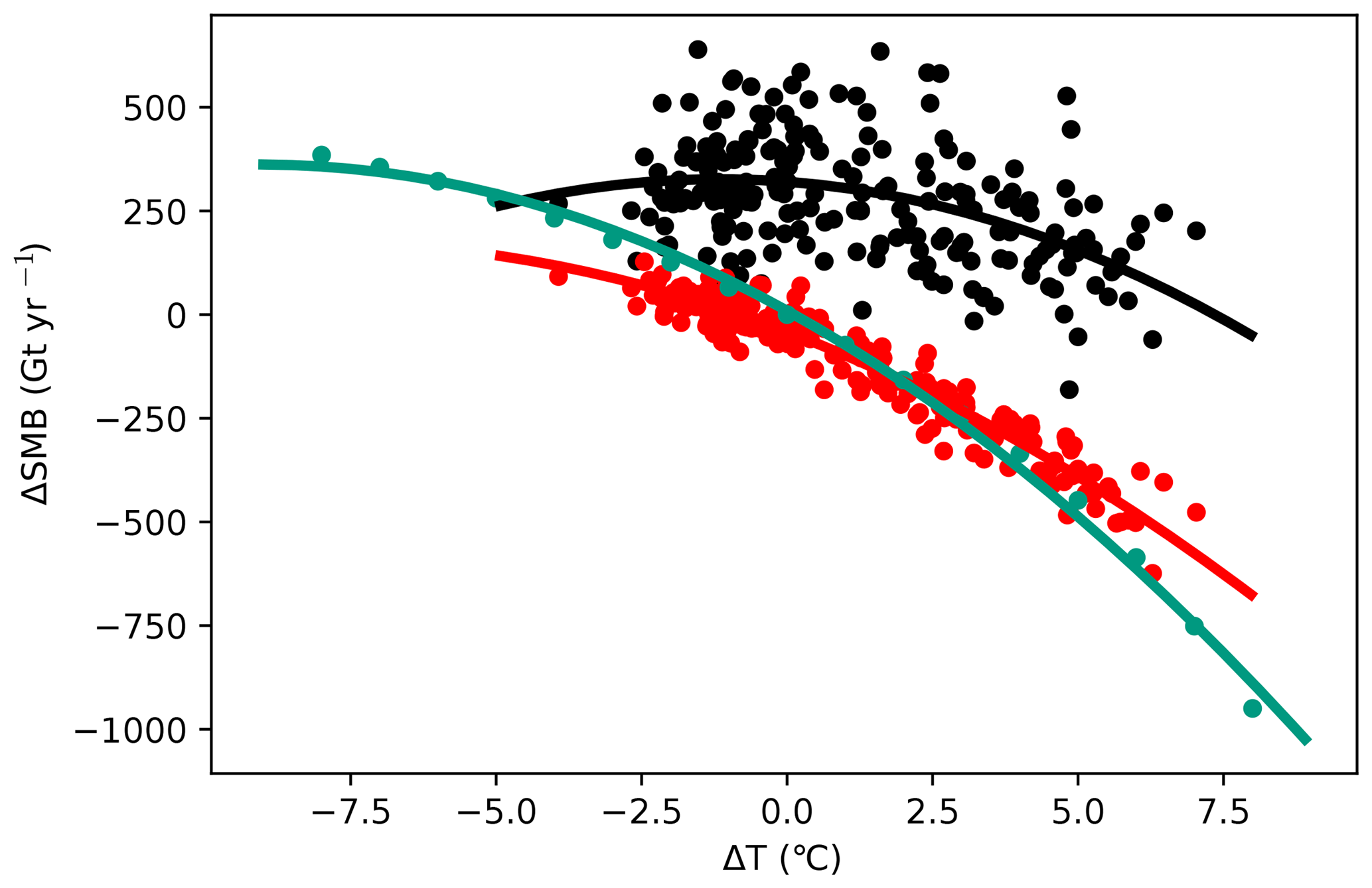
https://www.the-cryosphere.net/13/1529/2019/tc-13-1529-2019-f13

Figure 13Change in surface mass balance as a function of anomalous annual average temperature over Greenland. Colours represent a spatially uniform temperature anomaly (green), a temperature pattern derived from a particular simulation year of a climate model (red), and the same temperature anomaly accompanied with the corresponding precipitation anomaly (black). Curves represent a least-squares regression of order two.

Download

https://www.the-cryosphere.net/13/1529/2019/tc-13-1529-2019-f14

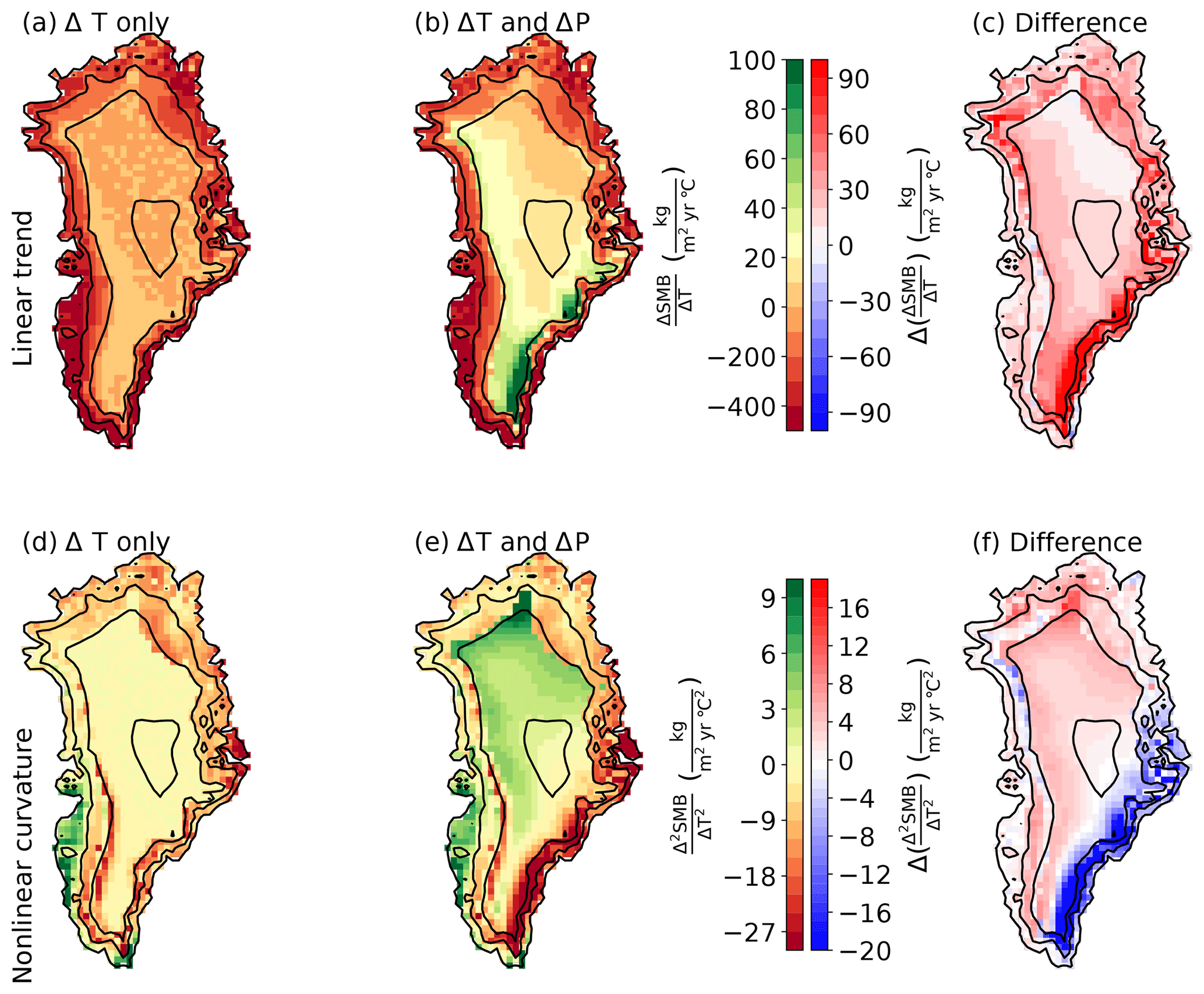
Figure 14Spatial distribution of linear trend (a, b) and curvature (d, e) of the SMB anomalies as a function of perturbations in the annual mean temperature for simulations that were perturbed with the temperature anomalies alone (a, d), simulations that were perturbed by both anomalous temperature and corresponding precipitation (b, e), and the respective differences (c, f).

Download

Repeating the parabolic regression for each surface grid point yields maps for the linear trend and curvature (Fig. 14). The simulations with a constant temperature offset are not included in this analysis. The linear trend of the SMB is negative everywhere on Greenland in the case that BESSI is forced only with anomalous temperatures. If the corresponding anomalies in precipitation are also taken into account, regions on the southeastern and western upper margins show an increase in mass balance with higher temperatures. This is because warm temperatures in these regions are often caused by the influx of relatively moist oceanic air masses. Similarly, the curvature of the temperature–SMB curve is negative everywhere on the ice sheet for temperature anomalies, whereas the combination of anomalous temperature and precipitation forcing results in positive curvatures in the interior. Interestingly, the largest negative curvature coincides with the region of positive trend, indicating that relatively small temperature anomalies cause an increase in SMB. The trend inverses quickly as soon as a certain threshold is passed. A similar pattern is seen for the integrated mass balance of the entire ice sheet (Fig. 13, black), which has important consequences for the stability of the ice sheet in a warmer climate.

6 Discussion and conclusions

We developed and calibrated the new surface energy and mass balance model BESSI that is optimized for long simulation times and for coupling with intermediate complexity climate models. The model domain includes all land areas in the Northern Hemisphere that were glaciated during the Pleistocene ice ages, at a lateral resolution of 40 km. The model has 15 vertical layers on a mass-following grid that covers the upper 15 m, approximately. With its three-dimensional domain, the physically accurate representation of surface energy fluxes, internal diffusion of heat, and the explicit tracking of liquid water and refreezing, BESSI combines features of complex SMB models (Reijmer and Hock, 2008; Steger et al., 2017) with a relatively coarse vertical resolution and a long time step. While it cannot match the numerical speed of empirical or more heavily parameterized models (Reeh, 1991; Robinson et al., 2010), BESSI simulates multiple centuries per hour on a modern personal computer, which fulfils our goal of developing a model that is capable of simulating multiple glacial cycles within a defensible amount of time. Although not included here, preliminary tests with an asynchronous time step promise to increase the speed by another order of magnitude. For this, the computation in regions with only seasonal snow and without liquid water is carried out only once every 50 years.

The simulated seasonal snow cover agrees well with satellite observations. Ice caps are reproduced well in different climate zones ranging from dry Arctic conditions in northern Greenland and on Svalbard to maritime climate on Iceland and in southeast Alaska and to the semi-arid continental climate of the Karakoram mountains. This demonstrates the robustness of the model to different boundary conditions and encourages future simulations with glacial climate. The surface energy and mass balance of the GrIS compare well to estimates from remote sensing.

The computational efficiency of the model enables large ensembles of simulations for calibration or to test the sensitivity to changes in the boundary conditions. As an example, we tested how the surface mass balance over Greenland depends on variations in surface air temperature, and the combined effect of when these temperature anomalies are accompanied by meteorologically coherent variations in precipitation. One key result is that such an increase in temperature does not lead to a decrease in net accumulation in all regions because the warmth comes from moist air masses that also bring snow. In addition to this positive linear trend, large parts of the interior of the GrIS have a positive curvature for the mass balance–temperature relationship. This means that, contrary to previous findings that only considered variability in temperature regardless of their meteorological implications (Mikkelsen et al., 2018), forcing the model with a variable climate may lead to a higher net accumulation compared to forcing with the climatological average.

The calibration revealed that the parameters for the atmospheric emissivity ϵ_air and the exchange of sensible heat D_sh have a strong influence on the model's performance. This is not ideal because both parameters simplify spatially heterogeneous processes with a globally uniform single value. This result points to some of the necessary compromises to build a fast model: a better representation of the sensible heat flux requires information on wind speed and a more realistic simulation of the downward longwave radiation are not possible without detailed information on the cloud cover and atmospheric moisture content. However, following our design goal to develop a model for simulations over multiple glacial cycles, these forcing fields were deliberately excluded, because for periods as far back as the last ice age they are only available from simulations of general circulation climate models. The computational cost of these climate models makes long simulation times infeasible. For the same reason, the physical processes of sublimation and windborne redistribution of snow are not included in BESSI.

Comparison with comprehensive models of the regional atmosphere and snow mass balance for Greenland showed that BESSI underestimates refreezing by a factor of 2, which leads to a negative bias in the total surface mass balance. This may be due to the relatively long time step of our model that neglects diurnal variations in temperature, as suggested recently by Krebs-Kanzow et al. (2018). It is possible that, although the model captures relative changes in mass balance due to the recent warming and interannual variability with reasonable detail in its current setting, the refreezing bias forces other model parameters to adopt values that negatively impact the model's sensitivity for longer simulations and under different boundary conditions. A more detailed study of the Greenland mass balance and its components will address these issues in the future.

Code availability

The source code of BESSI is available in the Supplement.

Supplement

The supplement related to this article is available online at: https://doi.org/10.5194/tc-13-1529-2019-supplement.

Author contributions

AB and MAI developed the model code with advice from TFS. AB and MAI designed and performed the experiments, analysed the output, and wrote the manuscript. TFS provided valuable input to the discussion at all stages.

Competing interests

The authors declare that they have no conflict of interest.

Acknowledgements

We are grateful to Jakob Schwander for his help with the firnification model and for providing snow density data for the NGRIP and NEEM sites. Reviews by Uta Krebs-Kanzow and Mario Krapp helped improve the quality of this study. Andreas Born is supported by a Starting Grant from the Bergen Research Foundation. Thomas F. Stocker acknowledges support by the Swiss National Science Foundation, project 200020-172745. Michael A. Imhof is supported by the Swiss National Science Foundation, project 200021-162444.

Financial support

This research has been supported by the Bergen Research Foundation and the Swiss National Science Foundation (grant nos. 200020-172745 and 200021-162444).

Review statement

This paper was edited by Alexander Robinson and reviewed by Uta Krebs-Kanzow and one anonymous referee.

References

Abe-Ouchi, A., Saito, F., Kawamura, K., Raymo, M. E., Okuno, J., Takahashi, K., and Blatter, H.: Insolation-driven 100,000-year glacial cycles and hysteresis of ice-sheet volume, Nature, 500, 190–193, https://doi.org/10.1038/nature12374, 2013. a

Amante, C. and Eakins, B. W.: ETOPO1 1 Arc-Minute Global Relief Model: Procedures, Data Sources and Analysis, Tech. rep., NOAA Technical Memorandum NESDIS NGDC-24, https://doi.org/10.7289/V5C8276M, 2009. a, b

Barnola, J. M., Pimienta, P., Raznaud, D., and Korotkevich, Y. S.: CO₂ climate relationship as deduced from the Vostok ice core: a reexamination based on new measurements and on a reevaluation of the air dating, Tellus, 43, 83–90, https://doi.org/10.1034/j.1600-0889.1991.t01-1-00002.x, 1991. a

Bartelt, P. and Lehning, M.: A physical SNOWPACK model for the Swiss avalanche warning Part I: numerical model, Cold Reg. Sci. Technol., 35, 123–145, 2002. a

Bonelli, S., Charbit, S., Kageyama, M., Woillez, M.-N., Ramstein, G., Dumas, C., and Quiquet, A.: Investigating the evolution of major Northern Hemisphere ice sheets during the last glacial-interglacial cycle, Clim. Past, 5, 329–345, https://doi.org/10.5194/cp-5-329-2009, 2009. a

Born, A.: Tracer transport in an isochronal ice sheet model, J. Glaciol., 63, 22–38, https://doi.org/10.1017/jog.2016.111, 2017. a

Born, A. and Nisancioglu, K. H.: Melting of Northern Greenland during the last interglaciation, The Cryosphere, 6, 1239–1250, https://doi.org/10.5194/tc-6-1239-2012, 2012. a

Bougamont, M., Bamber, J. L., and Greuell, W.: A surface mass balance model for the Greenland Ice Sheet, J. Geophys. Res., 110, 1–13, https://doi.org/10.1029/2005JF000348, 2005. a

Bougamont, M., Bamber, J. L., Ridley, J. K., Gladstone, R. M., Greuell, W., Hanna, E., Payne, A. J., and Rutt, I.: Impact of model physics on estimating the surface mass balance of the Greenland ice sheet, Geophys. Res. Lett., 110, F04018, https://doi.org/10.1029/2007GL030700, 2007. a

Box, J. E. and Steffen, K.: Sublimation weather on the Greenland ice sheet from automated station observations, J. Geophys. Res., 106, 33965–33981, https://doi.org/10.1029/2001JD900219, 2001. a

Braithwaite, R. J.: Calculation of sensible-heat flux over a melting ice surface using simple climate data and daily measurements of ablation, Ann. Glaciol., 50, 9–15, https://doi.org/10.3189/172756409787769726, 2009. a

Brodzik, M. J. and Armstrong, R.: Northern Hemisphere EASE-Grid 2.0 Weekly Snow Cover and Sea Ice Extent, Version 4. Boulder, Colorado USA. NASA National Snow and Ice Data Center Distributed Active Archive Center, https://doi.org/10.5067/P7O0HGJLYUQU, 2013. a

Busetto, M., Lanconelli, C., Mazzola, M., Lupi, A., Petkov, B., Vitale, V., Tomasi, C., Grigioni, P., and Pellegrini, A.: Parameterization of clear sky effective emissivity under surface-based temperature inversion at Dome C and South Pole, Antarctica, Antarct. Sci., 25, 697–710, https://doi.org/10.1017/S0954102013000096, 2013. a

Dee, D. P., Uppala, S. M., Simmons, A. J., Berrisford, P., Poli, P., Kobayashi, S., Andrae, U., Balmaseda, M. A., Balsamo, G., Bauer, P., Bechtold, P., Beljaars, A. C. M., van de Berg, L., Bidlot, J., Bormann, N., Delsol, C., Dragani, R., Fuentes, M., Geer, A. J., Haimberger, L., Healy, S. B., Hersbach, H., Hólm, E. V., Isaksen, L., Kållberg, P., Köhler, M., Matricardi, M., McNally, A. P., Monge-Sanz, B. M., Morcrette, J.-J., Park, B.-K., Peubey, C., de Rosnay, P., Tavolato, C., Thépaut, J.-N., and Vitart, F.: The ERA-Interim reanalysis: configuration and performance of the data assimilation system, Q. J. Roy. Meteor. Soc., 137, 553–597, https://doi.org/10.1002/qj.828, 2011. a

Fettweis, X., Franco, B., Tedesco, M., van Angelen, J. H., Lenaerts, J. T. M., van den Broeke, M. R., and Gallée, H.: Estimating the Greenland ice sheet surface mass balance contribution to future sea level rise using the regional atmospheric climate model MAR, The Cryosphere, 7, 469–489, https://doi.org/10.5194/tc-7-469-2013, 2013. a

Forster, R. R., Box, J. E., van den Broeke, M. R., Miège, C., Burgess, E. W., van Angelen, J. H., Lenaerts, J. T. M., Koenig, L. S., Paden, J., Lewis, C., Gogineni, S. P., Leuschen, C., and Mcconnell, J. R.: Extensive liquid meltwater storage in firn within the Greenland ice sheet, Nat. Geosci., 7, 95–98, https://doi.org/10.1038/ngeo2043, 2014. a

Gabbi, J., Carenzo, M., Pellicciotti, F., Bauder, A., and Funk, M.: A comparison of empirical and physically based glacier surface melt models for long-term simulations of glacier response, J. Glaciol., 60, 1140–1154, https://doi.org/10.3189/2014JoG14J011, 2014. a

Greuell, W.: Nummerical Modelling of the Energy Balance and the Englacial Temperature at the ETH Camp, West Greenland, Zürcher Geographische Schriften, 51, 1–81, 1992. a, b, c, d

Greuell, W. and Konzelmann, T.: Numerical modelling of the energy balance and the englacial temperature of the Greenland Ice Sheet. Calculations for the ETH-Camp location (West Greenland, 1155 m a.s.l.), Global Planet. Change, 9, 91–114, https://doi.org/10.1016/0921-8181(94)90010-8, 1994. a

Herron, M. M. and Langway Jr., C. C.: Firn densification: an empirical model, J. Glaciol., 25, 373–385, https://doi.org/10.3189/S0022143000015239, 1980. a

Hock, R.: Temperature index melt modelling in mountain areas, J. Hydrol., 282, 104–115, https://doi.org/10.1016/S0022-1694(03)00257-9, 2003. a

Krapp, M., Robinson, A., and Ganopolski, A.: SEMIC: an efficient surface energy and mass balance model applied to the Greenland ice sheet, The Cryosphere, 11, 1519–1535, https://doi.org/10.5194/tc-11-1519-2017, 2017. a

Krebs-Kanzow, U., Gierz, P., and Lohmann, G.: Brief communication: An ice surface melt scheme including the diurnal cycle of solar radiation, The Cryosphere, 12, 3923–3930, https://doi.org/10.5194/tc-12-3923-2018, 2018. a, b

Lehner, F., Joos, F., Raible, C. C., Mignot, J., Born, A., Keller, K. M., and Stocker, T. F.: Climate and carbon cycle dynamics in a CESM simulation from 850 to 2100 CE, Earth Syst. Dynam., 6, 411–434, https://doi.org/10.5194/esd-6-411-2015, 2015. a

Li, C. and Battisti, D. S.: Reduced Atlantic storminess during last glacial maximum: Evidence from a coupled climate model, J. Climate, 21, 3561–3579, https://doi.org/10.1175/2007JCLI2166.1, 2008. a

Liakka, J., Löfverström, M., and Colleoni, F.: The impact of the North American glacial topography on the evolution of the Eurasian ice sheet over the last glacial cycle, Clim. Past, 12, 1225–1241, https://doi.org/10.5194/cp-12-1225-2016, 2016. a

Merz, N., Born, A., Raible, C. C., Fischer, H., and Stocker, T. F.: Dependence of Eemian Greenland temperature reconstructions on the ice sheet topography, Clim. Past, 10, 1221–1238, https://doi.org/10.5194/cp-10-1221-2014, 2014a. a

Merz, N., Gfeller, G., Born, A., Raible, C., Stocker, T., and Fischer, H.: Influence of ice sheet topography on Greenland precipitation during the Eemian interglacial, J. Geophys. Res., 119, 10749–10768, https://doi.org/10.1002/2014JD021940, 2014b. a

Mikkelsen, T. B., Grinsted, A., and Ditlevsen, P.: Influence of temperature fluctuations on equilibrium ice sheet volume, The Cryosphere, 12, 39–47, https://doi.org/10.5194/tc-12-39-2018, 2018. a, b, c

Mote, T. L.: MEaSUREs Greenland Surface Melt Daily 25km EASE-Grid 2.0, Version 1. Boulder, Colorado USA. NASA National Snow and Ice Data Center Distributed Active Archive Center, https://doi.org/10.5067/MEASURES/CRYOSPHERE/nsidc-0533.001, 2014. a

Neff, B., Born, A., and Stocker, T. F.: An ice sheet model of reduced complexity for paleoclimate studies, Earth Syst. Dynam., 7, 397–418, https://doi.org/10.5194/esd-7-397-2016, 2016. a, b

Ohmura, A.: Physical Basis for the Temperature-Based Melt-Index Method, J. Appl. Meteorol., 40, 753–761, https://doi.org/10.1175/1520-0450(2001)040<0753:PBFTTB>2.0.CO;2, 2001. a

Paterson, W. S. B.: Physics of Glaciers, Butterworth-Heinemann, Oxford, UK and Woburn, MA, USA, 1999. a, b

Pellicciotti, F., Brock, B., Strasser, U., Burlando, P., Funk, M., and Corripio, J.: An enhanced temperature-index glacier melt model including the shortwave radiation balance: development and testing for Haut Glacier d'Arolla, Switzerland, J. Glaciol., 51, 573–587, https://doi.org/10.3189/172756505781829124, 2005. a

Plach, A., Nisancioglu, K. H., Le clec'h, S., Born, A., Langebroek, P. M., Guo, C., Imhof, M., and Stocker, T. F.: Eemian Greenland SMB strongly sensitive to model choice, Clim. Past, 14, 1463–1485, https://doi.org/10.5194/cp-14-1463-2018, 2018. a, b

Polashenski, C., Courville, Z., Benson, C., Wagner, A., Chen, J., Wong, G., Hawley, R., and Hall, D.: Observations of pronounced Greenland ice sheet firn warming and implications for runoff production, Geophys. Res. Lett., 41, 4238–4246, https://doi.org/10.1002/2014GL059806, 2014. a, b, c, d, e, f, g, h, i, j, k, l

Reeh, N.: Parameterization of melt rate and surface temperature on the Greenland Ice Sheet, Polarforschung, 59, 113–128, 1991. a, b

Reijmer, C. and Hock, R.: Internal accumulation on Storglaciären, Sweden, in a multi-layer snow model coupled to a distributed energy and mass balance model, J. Glaciol., 54, 61–72, https://doi.org/10.3189/002214308784409161, 2008. a, b

Reijmer, C. H., van den Broeke, M. R., Fettweis, X., Ettema, J., and Stap, L. B.: Refreezing on the Greenland ice sheet: a comparison of parameterizations, The Cryosphere, 6, 743–762, https://doi.org/10.5194/tc-6-743-2012, 2012. a

Ritz, S. P., Stocker, T. F., and Joos, F.: A Coupled Dynamical Ocean–Energy Balance Atmosphere Model for Paleoclimate Studies, J. Climate, 24, 349–375, https://doi.org/10.1175/2010JCLI3351.1, 2011. a, b

Robinson, A. and Goelzer, H.: The importance of insolation changes for paleo ice sheet modeling, The Cryosphere, 8, 1419–1428, https://doi.org/10.5194/tc-8-1419-2014, 2014. a

Robinson, A., Calov, R., and Ganopolski, A.: An efficient regional energy-moisture balance model for simulation of the Greenland Ice Sheet response to climate change, The Cryosphere, 4, 129–144, https://doi.org/10.5194/tc-4-129-2010, 2010. a, b

Robinson, A., Calov, R., and Ganopolski, A.: Greenland ice sheet model parameters constrained using simulations of the Eemian Interglacial, Clim. Past, 7, 381–396, https://doi.org/10.5194/cp-7-381-2011, 2011. a

Schwander, J.: Firn Air Sampling Field Report NORTH GRIP 2001, Tech. rep., University of Bern, Bern, Switzerland, 2001. a, b, c, d

Schwander, J., Sowers, T., Barnola, J.-M., Blunier, T., Fuchs, A., and Malaize, B.: Age scale of the air in the summit ice: Implication for glacial-interglacial temperature change, J. Geophys. Res., 102, 19483–19493, https://doi.org/10.1029/97JD01309, 1997. a

Schwander, J., Sowers, T., Blunier, T., and Petrenko, V.: Firn Air Sampling Field Report NEEM 2008, Tech. rep., University of Bern, Bern, Switzerland, 2008. a, b, c, d

Spratt, R. M. and Lisiecki, L. E.: A Late Pleistocene sea level stack, Clim. Past, 12, 1079–1092, https://doi.org/10.5194/cp-12-1079-2016, 2016. a

Steffen, K. and Box, J.: Surface climatology of the Greenland ice sheet: Greenland Climate Network 1995-1999, J. Geophys. Res., 106, 33951–33964, https://doi.org/10.1029/2001JD900161, 2001. a, b, c, d, e, f, g, h, i, j, k, l

Steger, C. R., Reijmer, C. H., and van den Broeke, M. R.: The modelled liquid water balance of the Greenland Ice Sheet, The Cryosphere, 11, 2507–2526, https://doi.org/10.5194/tc-11-2507-2017, 2017. a, b, c

van de Berg, W. J., van den Broeke, M., Ettema, J., van Meijgaard, E., and Kaspar, F.: Significant contribution of insolation to Eemian melting of the Greenland ice sheet, Nat. Geosci., 4, 679–683, https://doi.org/10.1038/ngeo1245, 2011. a

van den Broeke, M. R., Enderlin, E. M., Howat, I. M., Kuipers Munneke, P., Noël, B. P. Y., van de Berg, W. J., van Meijgaard, E., and Wouters, B.: On the recent contribution of the Greenland ice sheet to sea level change, The Cryosphere, 10, 1933–1946, https://doi.org/10.5194/tc-10-1933-2016, 2016. a, b

Vaughan, D. G., Comiso, J. C., Allison, I., Carrasco, J., Kaser, G., Kwok, R., Mote, P., Murray, T., Paul, F., Ren, J., Rignot, E., Solomina, O., Steffen, K., and Zhang, T.: Observations: Cryosphere, in: Climate Change 2013: The Physical Science Basis. Contribution of Working Group I to the Fifth Assessment Report of the Intergovernmental Panel on Climate Change, edited by: Stocker, T. F., Qin, D., Plattner, G.-K., Tignor, M., Allen, S. K., Boschung, J., Nauels, A., Xia, Y., Bex, V., and Midgley, P. M., 317–382, Cambridge University Press, Cambridge, UK and New York, NY, USA, 2013. a

Vionnet, V., Brun, E., Morin, S., Boone, A., Faroux, S., Le Moigne, P., Martin, E., and Willemet, J.-M.: The detailed snowpack scheme Crocus and its implementation in SURFEX v7.2, Geosci. Model Dev., 5, 773–791, https://doi.org/10.5194/gmd-5-773-2012, 2012. a

Watkins, M. M., Wiese, D. N., Yuan, D.-N., Boening, C., and Landerer, F. W.: Improved methods for observing Earth's time variable mass distribution with GRACE using spherical cap mascons, J. Geophys. Res.-Sol. Ea., 120, 2648–2671, https://doi.org/10.1002/2014JB011547, 2015. a

Wiese, D. N., Yuan, D.-N., Boening, C., Landerer, F. W., and Watkins, M. M.: JPL GRACE Mascon Ocean, Ice, and Hydrology Equivalent Water Height RL05M.1 CRI Filtered Version 2, PO.DAAC, CA, USA, https://doi.org/10.5067/TEMSC-2LCR5, 2016. a

Yen, Y.-C.: Review of thermal properties of snow, ice and sea ice, Tech. rep., Hanover, New Hampshire, USA, 1981. a

Articles

Short summary

We present a new numerical model to simulate the surface energy and mass balance of snow and ice. While similar models exist and cover a wide range of complexity from empirical models to those that simulate the microscopic structure of individual snow grains, we aim to strike a balance between physical completeness and numerical efficiency. This new model will enable physically accurate simulations over timescales of hundreds of millennia, a key requirement of investigating ice age cycles.