the Creative Commons Attribution 4.0 License.
the Creative Commons Attribution 4.0 License.
 | 22 Jan 2019
The optical characteristics and sources of chromophoric dissolved organic matter (CDOM) in seasonal snow of northwestern China
Jun Liu
Chromophoric dissolved organic matter (CDOM) plays an important role in the global carbon cycle and energy budget but is rarely studied in seasonal snow. A field campaign was conducted across northwestern China from January to February 2012, and surface snow samples were collected at 39 sites in Xinjiang and Qinghai provinces. Absorption and fluorescence spectroscopies, along with chemical analysis, were used to investigate the optical characteristics and potential sources of CDOM in seasonal snow. The abundance of CDOM, shown as the absorption coefficient at 280 nm, aCDOM(280), and the spectral slope from 275 to 295 nm (S275−295) ranged from 0.15 to 10.57 m−1 and 0.0129 to 0.0389 nm−1. The highest average aCDOM(280) (2.30±0.52 m−1) was found in Qinghai, and the lowest average S275−295 (0.0188±0.0015 nm−1) indicated that the snow CDOM in this region had a strongly terrestrial characteristic. The lower values of aCDOM(280) were found at sites located to the north of the Tianshan Mountains and northwestern Xinjiang along the border of China (0.93±0.68 m−1 and 0.80±0.62 m−1). Parallel factor (PARAFAC) analysis identified three types of fluorophores that were attributed to two humic-like substances (HULIS, C1 and C2) and one protein-like material (C3). C1 was mainly from soil HULIS, C3 was a type of autochthonously labile organic matter, while the potential sources of C2 were complex, including soil, microbial activity, anthropogenic pollution, and biomass burning. Furthermore, the regional variations of sources for snow CDOM were assessed by analyses of chemical species (e.g., soluble ions), fluorescent components, and air mass backward trajectories combined with satellite-derived active-fire locations.
- Article
(5778 KB) - Full-text XML
-
Supplement
(1014 KB) - BibTeX
- EndNote


Dissolved organic matter (DOM) is widely distributed in natural aquatic ecosystems and plays a key role in the global carbon cycle (Massicotte et al., 2017). Chromophoric dissolved organic matter (CDOM), widely known as the light-absorbing constituent of DOM, can absorb light from ultraviolet to visible (UV–vis) wavelengths (Bricaud et al., 1981). Owing to its light-absorbing properties, CDOM is important in biological processes (Seekell et al., 2015; Thrane et al., 2014), photochemical processes (Helms et al., 2013; Vaehaetalo and Wetzel, 2004), and the energy budget (Hill and Zimmerman, 2016; Pegau, 2002) in natural water bodies.
Compared to the aquatic environments, there were only limited studies evaluating DOM in the cryosphere. Whereas the global glacier ecosystem is a large organic carbon pool and exports approximately 1.04±0.18 TgC yr−1 of dissolved organic carbon into freshwater and marine environments (Hood et al., 2015). In addition, the glacier-derived DOM shows high bioavailability and can be a source of labile organic matter for downstream ecosystems (Hood et al., 2009; Lawson et al., 2014; Singer et al., 2012). The DOM in snow and ice originates from in situ processes (autochthonous) such as microbial activity (Anesio et al., 2009) and is imported from the surrounding terrestrial environments (allochthonous), including soil, vegetation (Bhatia et al., 2010), and anthropogenic activity (Stubbins et al., 2012).
Snowfall is an important carbon and nutrient input for land ecosystems (Mladenov et al., 2012) and a crucial freshwater reservoir (Jones, 1999). Snowpack is also an active field for photochemical (Beine et al., 2011; Domine et al., 2013) and biological processes (Liu et al., 2009; Lutz et al., 2016). Unlike the aquatic environments, high surface albedo is the most obvious physical property of snow (IPCC, 2013). Once light-absorbing impurities are deposited on the snow surface, the albedo can be significantly reduced, and the regional and global climate are further affected (Hadley and Kirchstetter, 2012). Several field campaigns covering the Arctic, Russia, North America, and northern China have been conducted to measure insoluble light-absorbing particles (ILAPs) in snow, for instance black carbon (BC), insoluble organic carbon (ISOC), and mineral dust (MD) (Doherty et al., 2010, 2014, 2015; Huang et al., 2011; Pu et al., 2017; Wang et al., 2013, 2015, 2017; Warren and Wiscombe, 1980; Ye et al., 2012; Y. Zhou et al., 2017). However, these studies neglected CDOM, which is rarely studied in snow but has been proven to be an effective light absorber whether in the atmosphere (i.e., brown carbon, BrC) (Hecobian et al., 2010) or in water bodies (Bricaud et al., 1981). To constrain the photochemistry of snow soluble chromophores, Anastasio and Robles (2007) first quantified the light absorption of dissolved chromophores in melted snow samples from the Arctic and Antarctica. They found that in addition to and H2O2, approximately half of the light absorption at 280 nm and above was due to unknown chromophores, probably organics. After that, Beine et al. (2011) analyzed more than 500 snow samples collected in Alaska. They exhibited slight contributions of H2O2 and to the total absorption within 300–450 nm (combined <9 %), while humic-like substances (HULIS), which are a type of macromolecular organic matter defined for aerosol with certain similar chemical properties to terrestrial and aquatic humic and fulvic substances (Graber and Rudich, 2006), and unknown chromophores each accounted for approximately half of the total absorption. Recently, several studies have started to focus on the optical properties and radiative forcing of CDOM in glaciers on the Tibetan Plateau. Yan et al. (2016) measured the mass absorption cross section (MAC) of CDOM in snow (1.4±0.4 m2 g−1 at 365 nm) at Laohugou Glacier, northern Tibetan Plateau, and further calculated the radiative forcing of CDOM, which accounted for approximately 10 % relative to that of BC. Niu et al. (2018) showed quite a high MAC value of CDOM (6.31±0.34 m2 g−1 at 365 nm) in snow and ice samples collected on Mt. Yulong, southeastern Tibetan Plateau. Moreover, it is surprising that the light absorption of CDOM within 330 to 400 nm was approximately 4 times higher than that of BC, although with high uncertainty. In above studies, CDOM showed significant effects on the energy budget of surface snow and ice on glaciers. Until now, the study of CDOM in snow and ice is still in its infancy, and much more work is imperative to improve our understanding of it. In northern China, snowpack is affected by more anthropogenic activities or sunlight than those at higher elevation or latitude, thus the effects of CDOM may be more remarkable. Therefore, we conducted a large field campaign to investigate the CDOM in seasonal snow of northwestern China from January to February 2012.
UV–vis absorption and fluorescence spectroscopies are both rapid and effective methods for characterizing the optical properties and sources of CDOM. The absorption coefficient at a certain wavelength within the UV band, for instance, 254, 280, or 350 nm (Spencer et al., 2012; Zhang et al., 2010, 2011), usually serves as an indicator of CDOM abundance. The absorption spectrum of CDOM decreases approximately exponentially with increasing wavelength (Helms et al., 2008), and is usually described by the spectral slope (S) (Twardowski et al., 2004). Helms et al. (2008) used the spectral slope between 275 and 295 nm (S275−295) to investigate the molecular weight and sources of CDOM (terrestrial or marine origin), i.e., lower S275−295 corresponds to CDOM with a higher molecular weight and a more obviously terrestrial characteristic. Fluorescence excitation–emission matrix (EEM) has been widely used to identify the sources and compositions (humic-like or protein-like) of fluorescent DOM (FDOM) in natural waterbodies (Birdwell and Engel, 2010; Coble, 1996; Zhao et al., 2016), rainwater (Y. Q. Zhou et al., 2017), fog water (Birdwell and Valsaraj, 2010), and aerosols (Duarte et al., 2004; Lee et al., 2013; Mladenov et al., 2011). To precisely extract useful information from the large data set of EEMs, Bro (1997) successfully applied parallel factor (PARAFAC) analysis to decompose EEMs into several independent fluorescent components. Due to the great advantages of PARAFAC analysis in interpreting the results of EEMs, this has been the mainstream approach in recent natural CDOM studies (Murphy et al., 2013). However, the application of EEM combined with PARAFAC analysis in the cryosphere is scarce. Therefore, we try to employ it to characterize the snow CDOM.
In this study, for the first time, with the aim of presenting a comprehensive understanding of CDOM in seasonal snow across northwestern China, UV–vis absorption and fluorescence spectroscopies along with chemical analysis were applied to investigate the abundances, optical properties, and potential sources of CDOM as well as their spatial distributions.
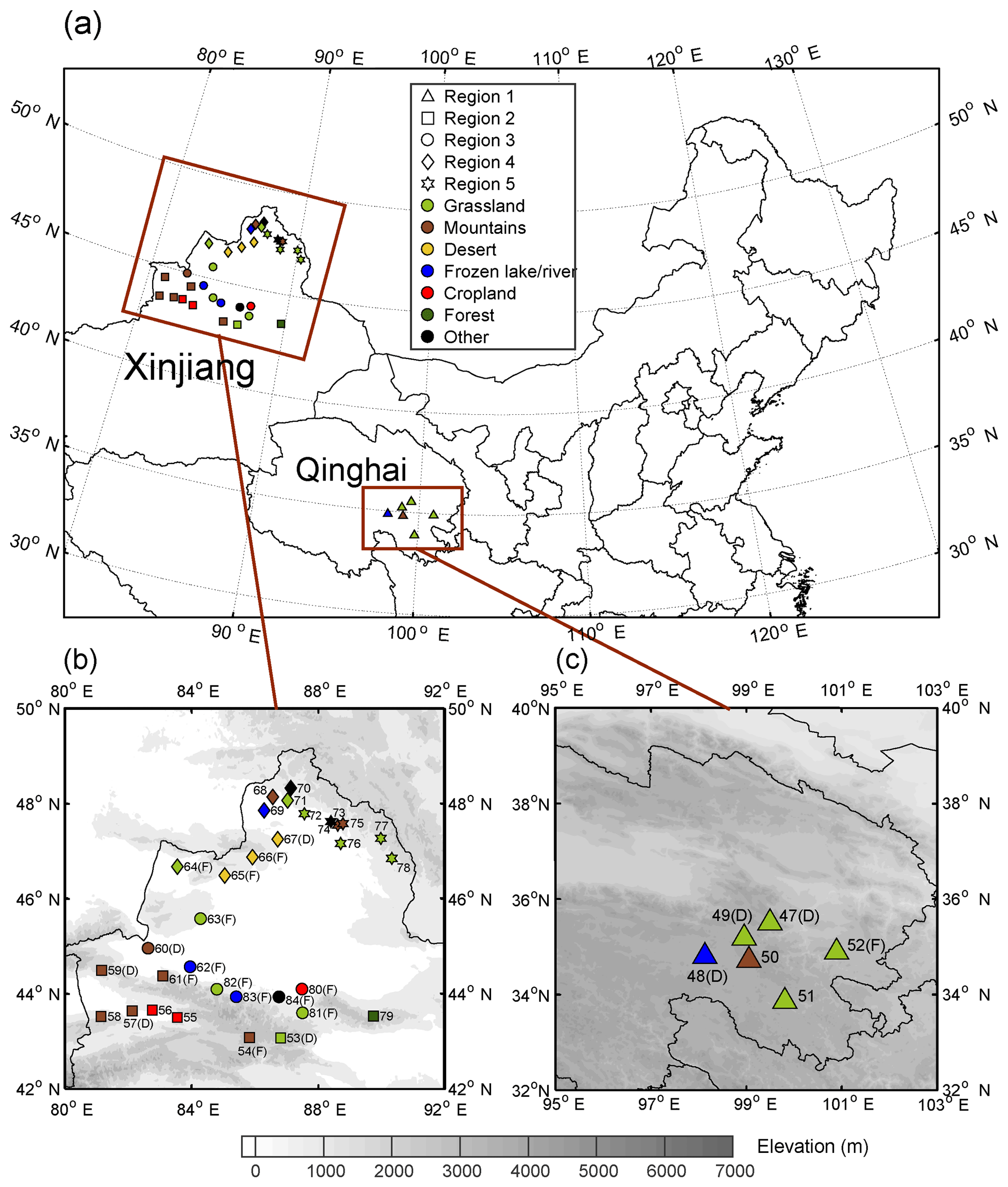
Figure 1(a) Location of study area and sample site distribution across northwestern China. The site numbers and regional groupings are shown in panel (b) for Xinjiang and (c) for Qinghai. Sample sites are divided into five groups indicated by different symbols, and the land cover types are represented in different colors, as shown in the legend in panel (a). The D indicates that the sample was collected from a snow drift, and the F indicates that the sample was fresh snow. The elevation is shown in the contour plot.
2.1 Sample collection
During January to February 2012, snow samples were collected at 7 sites in Qinghai and 32 sites in Xinjiang, northwestern China. The distribution of sample sites, which are numbered chronologically, is shown in Fig. 1. Based on Pu et al. (2017), these sites were separated into five regions by their geographical distribution to investigate the spatial variations of light absorption and fluorescence properties, as well as the potential sources of CDOM. Region 1 is in the southeastern part of Qinghai at high altitude, and other regions are in Xinjiang. Region 2 is along the Tianshan Mountains; region 3 is located to the north of the Tianshan Mountains and close to the industrial city belt in central Xinjiang. Regions 4 and 5 are in northwestern and northeastern Xinjiang, and both are along the border of China.
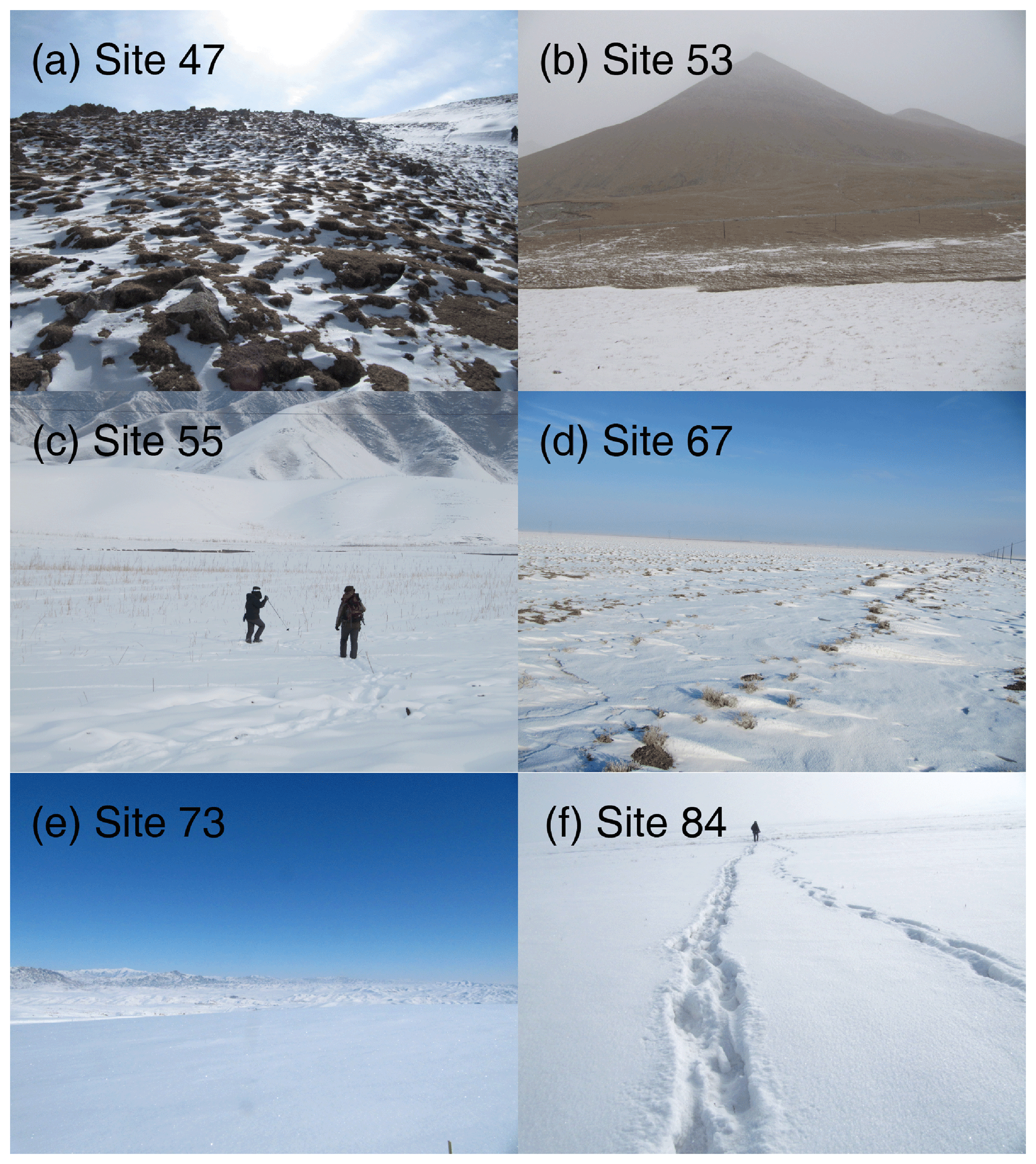
The sample sites were chosen to be upwind and far enough away from roads, railways, cities, and villages to minimize the effects of local pollution. Hence, the collected samples can be representative of a wide range of areas. Pictures of several sample sites are shown in Fig. 2. Snow samples were collected every 5 cm from top to bottom at each site. If there was a melt layer or fresh snow on the top layer, such a sample was collected individually. A pair of two adjacent vertical profiles of snow (left and right samples) to assess the variability of the same snowpack and to enhance the accuracy of the measurements. During this campaign, 13 fresh snow samples that had fallen during the sampling time were collected. In addition, at some sites, the snow was thin and patchy and the wind was strong; hence, these samples were gathered from snow drifts and were potentially influenced by the deposition of local soil dust (Ye et al., 2012). More details on the sampling methods have been reported previously (Doherty et al., 2010; Wang et al., 2013; Ye et al., 2012).
After being returned to the laboratory in Lanzhou University, all the samples were stored in a freezer at −20 ∘C or lower for subsequent analyses. However, some previous studies indicated that the freeze–thaw process may lead to biases of the optical properties for DOM samples. For instance, Fellman et al. (2008) reported that there was a decrease in specific ultraviolet absorbance (SUVA) for stream water DOM after frozen, with a median of approximately 8 %. A study of peatland DOM found that the change in light absorption at 254 nm after freeze and thaw was less than 5 % of the median (Peacock et al., 2015). Thieme et al. (2016) assessed the changes in fluorescence properties for several types of DOM sample. The results showed the decreased relative percentages of terrestrial humic-like fluorophores (−3 % on average) and humification index (HIX, −2 % on average), and the increased percentage of fluvic-like fluorophore (+6 % on average). Other studies have also shown that the optical properties (light absorption and fluorescence) of several types of DOM were not affected significantly by freezing, such as those in ocean water, pore water, spring, and cave water (Birdwell and Engel, 2010; Del Castillo and Coble, 2000; Otero et al., 2007; Yamashita et al., 2010). As discussed above, the freeze–thaw process may influence the relative contributions of PARAFAC components slightly, while the effects on aCDOM(280) and fluorescence indices can be neglected.
2.2 Fluorescence measurement
The snow samples were first melted under room temperature. Then, the meltwater samples were filtrated using 0.22 µm PTFE syringe filters (Jinteng, Tianjin, China) and stored in pre-baked glass vials (450 ∘C for 4 h) at 4 ∘C in a freezer. All the samples were measured for UV–vis and fluorescence spectroscopies within 24 h after filtration. The ultrapure water (18.2 MΩ cm) filtrated by the PTFE syringe filters exhibited no clear fluorescence signal.
The EEMs (n=78) of surface snow samples were measured by an Aqualog spectrofluorometer system (Horiba Scientific, NJ, USA) in a 1 cm quartz cell. The scanning ranges were 240 to 600 nm in 5 nm intervals for excitation and 250 to 825 nm in 4.65 nm (8 pixels) intervals for emission, with the integrating time of 5 s. An ultrapure water blank was subtracted to remove the water Raman scatter peaks.
The inner filter effect (IFE) of EEM was corrected using the method shown in Kothawala et al. (2013). The fluorescence intensities were calibrated by the Raman peak of ultrapure water reference at a 350 nm excitation wavelength following the method presented by Lawaetz and Stedmon (2009). The Rayleigh scatter peaks were addressed by the EEMscat MATLAB toolbox (version 3) using an interpolation algorithm (Bahram et al., 2006).
PARAFAC is a multi-way method for modeling the data with three- or higher-order arrays (Murphy et al., 2013). For EEMs, the three dimensions are samples, excitation, and emission wavelengths. PARAFAC analysis can decompose the EEMs into several components with clear chemical interpretations. The details about the theory of PARAFAC analysis can be found in the Supplement. In this study, PARAFAC analysis was performed using the DOMFluor toolbox (version 1.7, Stedmon and Bro, 2008) in MATLAB. In addition, because the emission signals were mainly in the range of 250–650 nm, those at longer wavelengths were weak and more likely to be noises; hence, the emission wavelengths longer than 650 nm were not considered in the model. According to the analysis of residual error, split-half method, and visual inspection, the three-component PARAFAC model was selected. The residual error decreased distinctly when the component number increased from two to three and from four to five (Fig. S1). Combined with the split-half analysis for 2- to 7-component models, only 2- and 3-component models were validated with the S4C4T2 split scheme (Murphy et al., 2013). Therefore, the 3-component model was chosen here. The fluorescence intensity of each fluorescent component was expressed as Fmax in Raman unit (RU) (Stedmon and Markager, 2005b). The relative contributions of intensities for three components to the total fluorescence are given as %C1–%C3 hereinafter. In addition, three fluorescence-derived indices are widely used to identify the potential sources of CDOM. Zsolnay et al. (1999) presented HIX to describe the relative humification of DOM. The fluorescence index (FI) is used to identify the sources of DOM from terrestrial or microbial origins (McKnight et al., 2001), and the biological index (BIX) can be an indicator of autochthonous productivity (Huguet et al., 2009). These three indices are calculated by the following formulas:
where I is the fluorescence intensity, and Ex and Em are short for the excitation and emission wavelengths. We note that the wavelengths used in the calculation were changed slightly (1 nm or less) due to different instruments.
2.3 UV–vis absorption measurement
The UV–vis absorption spectra (n=78) of snow samples were derived from 240 to 600 nm in 5 nm intervals, while the fluorescence measurements were conducted by an Aqualog spectrofluorometer system, and an ultrapure water blank was used as a reference. The absorbance of CDOM was assumed to be zero above 550 nm, and the average absorbance between 550 and 600 nm was subtracted from the whole spectrum to correct the baseline shifts and scattering effects of the measurement. The absorbances of samples were converted to absorption coefficients using the following equation:
where A is the absorbance, λ is the wavelength, L is the path length of cuvette (0.01 m), and aCDOM is the absorption coefficient (m−1). The abundance of CDOM is presented by the absorption coefficient at 280 nm, aCDOM(280) (Zhang et al., 2010). The S275−295 was determined both by a log-transform linear regression and an exponential regression. The variation of these two methods was approximately 3 % on average. Linear regression has been frequently used to calculate S275−295 (Fichot and Benner, 2012; Helms et al., 2008; Yang et al., 2013), and in this study, showed higher R2 values than exponential regression. Therefore, the results of linear regression were adopted here. Additionally, if the difference in S275−295 between the linear and exponential methods was higher than 10 %, indicating a high uncertainty for absorption measurement, such data were removed. The absorption Ångström exponent (AAE) is used to describe the wavelength dependence of light absorption for aerosol (Bond, 2001), which has also been applied to characterize the ILAPs and CDOM in snow and ice (Doherty et al., 2010; Niu et al., 2018; Wang et al., 2013; Yan et al., 2016). The AAEs were calculated using power-law regression in the wavelength range of 240 to 550 nm, as follows:
where K is a constant related to DOM concentration. The R2 of all regressions (S275−295 and AAE) were higher than 0.9 and most of them were higher than 0.95.
Because the light absorption within the visible wavelengths of some samples were below the detection limit of the spectrophotometer, 19 of 39 samples were available for the calculations of AAE.
Note that the left samples of sites 51b and 58, which showed abnormal absorption and fluorescence spectra compared to other samples, were supposed to be contaminated, and thereby these two samples were not considered for the absorption and fluorescence analyses.
2.4 Soluble ions
The major soluble ions of meltwater samples were analyzed with an ion chromatograph (Dionex, Sunnyvale, CA, USA) using an AS11 column for the anions , , Cl−, and F− and a CS12 column for the cations Na+, K+, Ca2+, Mg2+, and . The soluble ions showed no obvious differences between filtered and unfiltered samples (Pu et al., 2017). According to Pio et al. (2007), the K+ can be separated into three fractions: sea salt (ss), dust, and others (the fraction not related to sea salt and mineral dust, nss-ndust). The nss-ndust-K+ is a good marker for biomass burning (Pio et al., 2007). The Ca2+ concentrations of our samples were mostly higher than that of Na+, leading to much larger mass ratios of than that in seawater (0.038) (Pio et al., 2007). Therefore, Ca2+ is dominated by the dust fraction and not corrected to nss-Ca2+ in this study. nss-ndust-K+ is calculated using the following formulas (Pio et al., 2007):
In Eq. (7), 0.038 is the mass ratio of in seawater (Pio et al., 2007). In Eq. (8), the lowest mass ratio of of our samples (0.14) is used to evaluate the dust fraction of Na+. Similarly, the lowest mass ratio of (0.028) is used in Eq. (9) to calculate the dust fraction of K+.
2.5 Hierarchical cluster analysis
A hierarchical cluster analysis was used to classify the samples based on the relative abundances of three PARAFAC components. Euclidean distance was used to estimate the distances between samples. Before determining the clustering method, the cophenetic correlation coefficients, criteria for assessing the efficiency of clustering methods (Saracli et al., 2013), for the cluster trees created by different methods were calculated, including unweighted average, weighted average, centroid, farthest neighbor, shortest neighbor, weighted center of mass, and Ward's methods. Finally, the unweighted average method was chosen due to the highest cophenetic correlation coefficients. A total of four clusters were determined and labeled as clusters A–D.
2.6 Air mass backward trajectories and active-fire data
Air mass backward trajectory has been widely used to identify the sources of air pollution (Stein et al., 2015) and also successfully applied to studies of impurities in snow (Hegg et al., 2010; Wang et al., 2015; Zhang et al., 2013). In this study, 72 h air mass backward trajectories were conducted by the HYbrid Single-Particle Lagrangian Integrated Trajectory (HYSPLIT) model (version 4, http://ready.arl.noaa.gov/HYSPLIT.php, last access: 5 April 2018). The model was run at 500 m above ground level (a.g.l.) 4 times a day for a period of 30 days preceding the sampling date at a given site. Using a satellite map of fire locations, the backward trajectories that pass through the satellite-derived fire locations can be identified as the sources of biomass-burning particles to the receptor sites (Antony et al., 2014; Hegg et al., 2010; Zhang et al., 2013). We used the active-fire data from the Moderate Resolution Imaging Spectroradiometer (MODIS) Collection 6 (MCD14DL, 2018) and the Visible Infrared Imaging Radiometer Suite (VIIRS) (VNP14IMGTDL_NRT, 2018) to capture potential fire location distributions. The data are available online: http://earthdata.nasa.gov/firms (last access: 2 October 2018).

Figure 3aCDOM(280) and S275−295 for sites in (a, c) Xinjiang and (b, d) Qinghai. The five regions are indicated by different symbols (same as Fig. 1).
3.1 The absorption characteristics of CDOM (aCDOM(280), S275−295, and AAE)
The distributions of aCDOM(280) and S275−295 are shown in Fig. 3, and the corresponding values are summarized in Table 1. aCDOM(280) ranged widely from 0.15 to 10.57 m−1 with an average of 1.69±1.80 m−1 (mean ± standard deviation). The highest value appeared at site 67 (10.57 m−1), followed by sites 53, 79, and 47 (5.25, 3.13, and 3.11 m−1). Most of these samples were collected from snow drifts. These values were higher than the aCDOM(280) of CDOM in snow, ice, and cryoconite on the Tibetan Plateau (typically lower than 2.0 m−1) (Feng et al., 2016, 2017). The lowest value was found at site 66 (0.15 m−1), followed by sites 70, 82, 73, and 83 (0.21, 0.23, 0.30, and 0.31 m−1), and these values were comparable with the absorption of soluble species in Alaskan snow with typical values of 0.1–0.15 m−1 at 250 nm (Beine et al., 2011). Some of these samples comprised freshly fallen snow and some were collected at remote sites that were far from pollution sources (Pu et al., 2017). The values of S275−295 ranged from 0.0129 to 0.0389 nm−1 with an average of 0.0243±0.0073 nm−1. S275−295 has never been reported in the terrestrial snow and ice samples before but is widely measured in the aquatic environments. For example, Hansen et al. (2016) summarized the S275−295 for oceanic and terrestrial water systems. The values are in the range of 0.020–0.030 nm−1 for ocean, 0.010–0.020 nm−1 for coastal water, and 0.012–0.023 nm−1 for rivers and wetlands. The S275−295 in this study covered the typical values in different types of natural water bodies, indicating complex compositions and sources of CDOM in seasonal snow across northwestern China. The AAEs of 19 CDOM samples are also shown in Table 1, which ranged from 4.41 to 8.91 with an average of 5.55±1.11. This value is comparable with the average AAE of HULIS extracted from Alaskan snow (6.11, from 300 to 550 nm) (Voisin et al., 2012).
Table 1Statistics on absorption and fluorescence parameters for snow CDOM at each site. Note that N.A. stands for no data.

The detailed results of each region are discussed below. Region 1 (sites 47–52) is located in the eastern Tibetan Plateau, which is typically higher than 4000 m above sea level. In this region, the snowpack is usually patchy and thin (Fig. 2a). During windy weather, local soil can be blown and deposited on the snow surface, which had been observed by previous studies (Pu et al., 2017; Ye et al., 2012). Moreover, the filters for samples in this region were in yellow due to the high loading of soil dust. The average aCDOM(280) was the highest among all five regions (2.30±0.52 m−1), and the S275−295 fell in the range of 0.0170–0.0212 nm−1 (0.0188±0.0015 nm−1), which shows similar values of leaching for permafrost on the Tibetan Plateau (Wang et al., 2018).
In region 2 (sites 53–59, 61, and 79), snow at some sites was patchy (e.g., sites 53, 57, 61, and 79, Fig. 2b), and some sites were farmland (e.g., sites 55 and 56, Fig. 2c), which can all be influenced by local soil due to strong wind. The aCDOM(280) values of these sites were in the range of 1.38–5.25 m−1. Several sites in this region showed lower aCDOM(280) (0.41–0.54 m−1, e.g., sites 54, 58, and 59) might result from new-fallen snow or fewer human activities due to their high altitude. Overall, region 2 showed a high average aCDOM(280) (2.00±1.50 m−1), and the average S275−295 was 0.0229±0.0073 nm−1.
Region 3 (sites 60, 62, 63, and 80–84) is the most developed part of Xinjiang, and major industrial cities are located here (e.g., Urumqi, Shihezi, Kuytun, and Karamay). Therefore, human activities may dominate the contribution of snow CDOM in this region. However, the aCDOM(280) values were mostly less than 1.0 m−1 except at sites 60 and 84, with a low average of 0.93±0.68 m−1. Because samples of these sites were almost new-fallen snow, the deposition of pollutants to the snowpack can be quite slight. Sites 60 and 84 were both close to industrial cities (Fig. 1 in Pu et al., 2017), and locally anthropogenic pollutants may be responsible for the high aCDOM(280) (2.39 and 1.65 m−1). The average S275−295 was 0.0218±0.0057 nm−1 in this region.
In region 4 (sites 64–71), the maximum and minimum aCDOM(280) values of the entire campaign were found here, i.e., 10.57 m−1 (site 67, snow drift, Fig. 2d) and 0.15 m−1 (site 66, new snow). Generally, the aCDOM(280) was in the range of 0.50–2.00 m−1 with an average of 0.80±0.62 m−1 (excluding site 67), which was the lowest of the values in all regions. The mean value of S275−295 (0.0255±0.0060 nm−1) was higher than those in regions 1–3.
In region 5 (sites 72–78), the average value of aCDOM(280) was 1.17±0.63 m−1, which was intermediate among five regions. S275−295 was typically higher than 0.0300 nm−1 and showed the highest average of 0.0324±0.0060 nm−1.

3.2 The fluorescence characteristics of CDOM
3.2.1 PARAFAC components
The EEMs of snow samples were analyzed by PARAFAC model, and three fluorescent components (C1–C3) were identified (Fig. 4). The corresponding excitation and emission loading spectra of each component are shown in Fig. S2. The excitation–emission (Ex–Em) wavelengths of each component's fluorescence peaks are summarized in Table 2.
Table 2Descriptions of fluorescent components identified by PARAFAC analysis. The secondary peaks are shown in parentheses.

C1 showed a primary peak at <240/453 nm for Ex–Em, which was similar to the component 1 reported by Stedmon and Markager (2005b) (Ex–Em = <250/448). This kind of fluorophore absorbs light mainly in the UVC band and shows a broad emission peak, which is usually identified as a terrestrial FDOM (Stedmon et al., 2003). The appearance of a secondary peak at longer excitation wavelength (Ex–Em = 305/453 nm) may indicate that C1 is more aromatic and has a higher molecular weight (Coble et al., 1998). C1 also resembled another terrestrial fluorophore, namely component 4 in Stedmon and Markager (2005b) (Ex–Em = <250(360)/440), which has been widely found in natural freshwater environments and even water-extracted organic matter in aerosols (Chen et al., 2016; Mladenov et al., 2011; Zhang et al., 2009; Zhao et al., 2016).
C2 had a primary (secondary) peak at <240(300)/393 nm (Ex–Em), which was first measured in the oceanic system by Coble (1996). Subsequently, Stedmon et al. (2003) found a similar fluorophore (component 4 therein) in a terrestrially dominated estuary region. The following studies suggested that the C2-like components are also linked to microbial activity and phytoplankton degradation in natural aquatic systems (Yamashita et al., 2008; Zhang et al., 2009) or DOM in waste water from anthropogenic sources (Stedmon and Markager, 2005b).
C3 is a typical fluorophore that is categorized as tyrosine-like FDOM and that exhibits Ex–Em pairs of <240(270)/315 nm. C3 reflects autochthonously labile DOM produced by biological processes (Stedmon et al., 2003) and has been commonly reported in previous studies of natural water bodies and water extraction of aerosols (Chen et al., 2016; Murphy et al., 2008; Stedmon and Markager, 2005a).

Figure 5Variations of fluorescent components among regions. The box plots show the Fmax of different components. The boxes denote the 25th and 75th quantiles, and the horizontal lines represent the 50th quantiles (medians), the averages are shown as dots; the whiskers denote the maximum and minimum data within 1.5 times the interquartile range, and the data points out of this range are marked with crosses (+). The pie charts show the regionally average relative contributions of three components. C1, C2, and C3 are represented in red, yellow, and blue, both for the box plots and pie charts. The percentages on the left of the panel are the averages of %C1–%C3 for the whole data set.
3.2.2 Regional variation in PARAFAC components
Figure 5 shows the variations of three fluorescent components among regions, including intensities and relative contributions. Overall, C2 was the most intense fluorophore and accounted for 42 % on average of the total fluorescence intensity of all samples, followed by C3 (38 % on average) and C1 (20 % on average). Compared to glacial snow and ice samples, which were dominated by protein-like substances (Dubnick et al., 2010; Feng et al., 2016), the seasonal snow samples in this study showed fewer microbial characteristic. According to Thieme et al. (2016), although we might underestimate %C1 (approximately 3 %) and overestimate %C2 (approximately 6 %) due to the preservation artifacts, it only slightly changes the results shown here.
In Qinghai (region 1), the most obvious feature was that C1 accounted for approximately 35 % of the total fluorescence intensity on average. This value was significantly higher than that of the other regions. In contrast, %C3 was quite low (24 % on average). This result was mainly due to the high Fmax (C1) in region 1, since the regional variation of Fmax (C3) was slight (Fig. 5).
In Xinjiang (regions 2–5), %C1 varied by region, while %C2 and %C3 were roughly equal. In region 2, %C1 was also high (25 % on average). However, %C1 showed the lowest value (9 % on average) in region 3, where most of the samples were new-fallen snow (7 of 8 sites). The great difference between %C1 and %C2 in this region indicated different sources of these two humic-like components. In regions 4 and 5, %C1 were nearly double of that in region 3 (both were approximately 17 % on average).
At sites 54 and 82, the relative abundance of C3 exceeded 70 %, which was approximately two-fold higher than the average of the whole data set (38 %). This result can be explained in two ways: (1) lower inputs of C1 and C2, and (2) greater biological activities being available in the snowpack at these sites. We found lichens near these two sites (Fig. S3), providing evidence for the latter.
At site 67, the fluorescence intensities were highest among all samples (0.30, 0.39, and 0.38 RU for C1, C2, and C3), especially for C3. The average Fmax (C3) was 0.10 RU for all samples excluding site 67, with a low standard deviation of 0.02 RU, and this value was approximately one-fourth of that at site 67. Therefore, rather than owing to biological activity alone, the extremely high Fmax (C3) of site 67 may be due to other sources, for instance, some organic compounds released from diesel combustion may show similar spectra (Mladenov et al., 2011).

Figure 6Hierarchical cluster analysis based on the relative contributions of fluorescent components.
To assess the similarities and differences between samples, a hierarchical cluster analysis based on the relative intensities of fluorescent components was conducted (Fig. 6). The snow samples were separated into four clusters (clusters A–D) (Fig. S4). Samples classified into clusters A and B were dominant. The high %C1, which was 34 % on average, was the most remarkable feature of cluster A and led to a low %C3 (26 % on average). All samples in region 1 and most samples in region 2 were assigned to cluster A. For cluster B, %C1 was low (13 % on average), and %C3 (47 % on average) was slightly higher than %C2 (40 % on average). For the sites in northern Xinjiang (regions 4 and 5), most samples were classified into cluster B. The samples assigned to cluster C, including those of sites 60, 62, 69, 72, 76, and 84, showed the dominant contribution of C2 (57 % on average). Half of these samples were found in region 3, and the others were dispersed in regions 4 and 5. Cluster D contained only two samples from sites 54 and 82. The difference between cluster D and the others was an extremely high contribution of protein-like component C3 (73 % on average), which indicated the high bioavailability of snow CDOM.
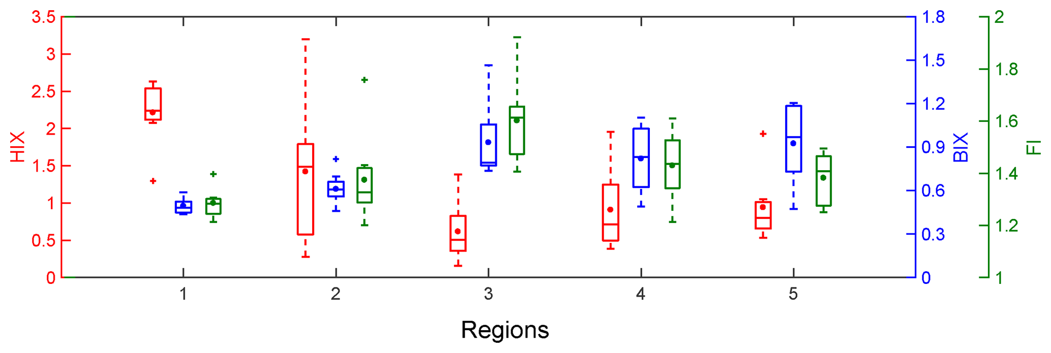
Figure 7Variations of HIX (red), BIX (blue), and FI (green) among regions. The meaning of each part of the box is same as that in Fig. 5.
3.2.3 Fluorescence-derived indices
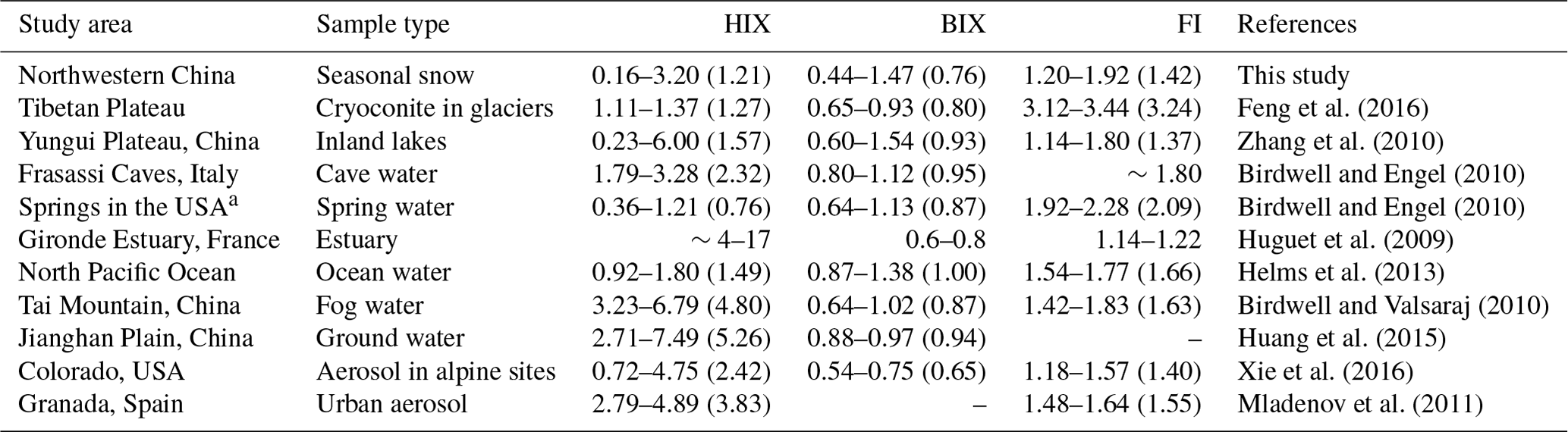
The regional variations of three established fluorescence-derived indices are shown in Fig. 7 and the values of each site are listed in Table 1. The HIX values fell into the range of 0.16–3.20, with an average of 1.21±0.78. The highest HIX appeared in region 1 (2.21±0.42), demonstrating a high degree of humification of snow CDOM. The lowest value was found in region 3 (0.62±0.37), which suggests that the CDOM was fresh. This finding is easily explained by the fact that nearly all snow samples in this region were new-fallen snow. Compared to other types of samples (Table 3), the HIX of snow CDOM across northwestern China was higher than that of spring water (Birdwell and Engel, 2010); comparable to those of cryoconite in glaciers from the Tibetan Plateau (Feng et al., 2016), inland lakes (Zhang et al., 2010), and North Pacific Ocean water (Helms et al., 2013); lower than those of cave water (Birdwell and Engel, 2010), estuarine water (Huguet et al., 2009), fog water (Birdwell and Valsaraj, 2010), groundwater (Huang et al., 2015), water extraction of alpine aerosol (Xie et al., 2016), and urban aerosol (Mladenov et al., 2011).
Table 3The fluorescence-derived indices in this study and comparison with those of natural water bodies and water extractions of aerosols reported by other studies. Note that average values are shown in parentheses.
a Including Jemez Spring, NM; Sharon Springs, NY; Sulfur Springs, IN; White Sulphur Springs, LA (Birdwell and Engel, 2010).
According to McKnight et al. (2001) and Huguet et al. (2009), the values of FI>1.9 or BIX>1.0 indicate microbially derived DOM. The BIX and FI for the snow samples were typically below 1.0 and 1.9, implying an unremarkably autochthonous characteristic. The regional distributions of BIX and FI corresponded with that of HIX. The samples with highest average BIX and FI were in region 3 (0.93±0.25 and 1.60±0.15), and the samples in region 1 exhibited the lowest average values (0.49±0.05 and 1.29±0.05). The BIX and FI of different types of samples changed little, while the only exception was the FI of cryoconite in glaciers from the Tibetan Plateau (Feng et al., 2016), which was approximately twice as high as those of the other samples.
3.3 Source attribution of CDOM
3.3.1 Source identification of PARAFAC components
As mentioned in Sect. 3.1, the snowpack in Qinghai was strongly influenced by local soil dust, which was confirmed by the lowest S275−295, leading to a high %C1. This result implied that the terrestrial fluorophore C1 was mainly from the soil HULIS, and demonstrated the invariably terrestrial source of the C1-like fluorophores, regardless of whether in the natural water bodies, aerosol water extraction, or snow.
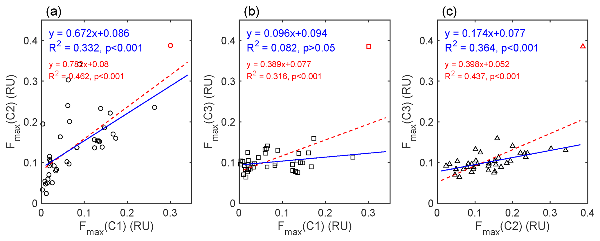
Figure 8Linear relationships between intensities of (a) C1 and C2, (b) C1 and C3, and (c) C2 and C3. The red dashed lines show the fits of the entire data set, and the blue solid lines show the fits of the data excluding site 67 (shown as markers in red). The corresponding fitting parameters are exhibited in the same color.
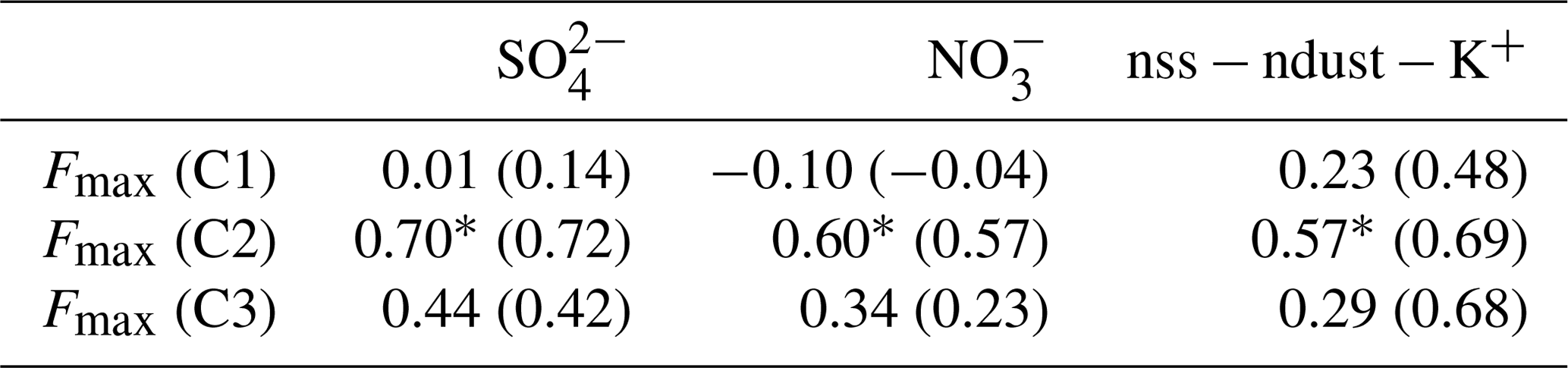
Correlation analyses were conducted to assess the potential sources of C2. The mutual relationships between PARAFAC components were shown in Fig. 8. The Fmax (C3) of site 67 was much higher than that of any other sample (shown as red markers in Fig. 8), which can strongly influence the results of the correlation analysis. When excluding the data of site 67, the R2 between Fmax (C1) and Fmax (C3) fell from 0.316 to 0.082, and the linear relationship became nonsignificant (Fig. 8b). Therefore, we used the data set that excludes site 67 in the analysis, and the results are shown below. Fmax (C1) and Fmax (C2) were linearly correlated with each other (R2=0.332, p<0.001); however, the R2 value was much lower than those in previous studies of natural water, for instance R2=0.63 for inland lakes (Zhao et al., 2016) and R2=0.88 for inland rivers (Zhang et al., 2011). This result indicated that soil dust only partly accounted for the source of C2. Meanwhile, a significant linear relationship (R2=0.364, p<0.001) was found between Fmax (C2) and Fmax (C3), which implied a potential microbial source for C2 and was consistent with the finding of Yamashita et al. (2008). Not surprisingly, Fmax (C1) and Fmax (C3) showed no correlation (R2=0.082, p>0.05). Furthermore, the correlation coefficients of Fmax and three major ions were calculated. The results are shown in Table 4. Fmax (C2) showed significant and positive correlations with these ions (p<0.001). The secondary ions and are commonly considered to be the markers of anthropogenic emissions from the burning of fossil fuel, such as oil and coal (Doherty et al., 2014; Oh et al., 2011; Pu et al., 2017), and nss−ndust is a good tracer of biomass burning (Pio et al., 2007). Therefore, C2 may also originate from anthropogenic pollution and biomass burning. Overall, there were four potential sources of snow CDOM in our study. Since the contribution of microbial-derived C3 to aCDOM(280) was relatively low compared to C1 and C2 (Fig. S5), three major sources were identified, i.e., soil dust, biomass burning, and anthropogenic pollution.
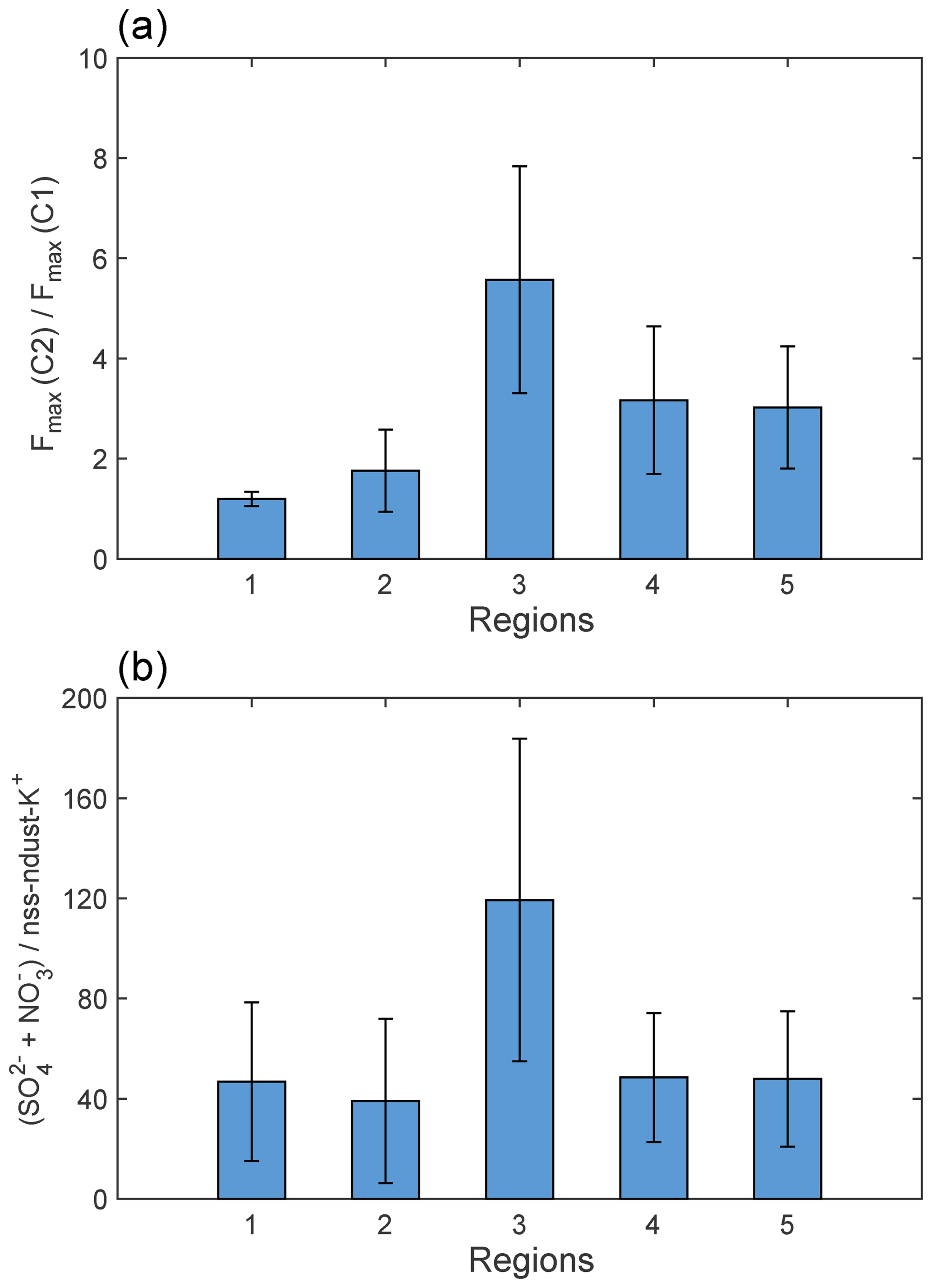
Table 4Pearson's correlation coefficients (r) of major ions and Fmax for fluorescent components when excluding the data from site 67; the results for the entire data set are shown in parentheses. Note that ∗ denotes p<0.001.
The ratios of intensities for PARAFAC components can be a useful tool for tracing the CDOM sources (Murphy et al., 2008). In this study, the ratio of Fmax (C2) and Fmax (C1) was applied to assess the relative contributions of soil and nonsoil (i.e., biomass burning and anthropogenic pollution) sources for snow CDOM (Fig. 9a). An analysis of variations (ANOVA) was used to test the differences among regions. Regions 1 and 2 showed low ratios of Fmax (C2) and Fmax (C1) (1.20±0.14 and 1.76±0.82), indicating the strong influence from local soil dust. The values of Fmax (C2)/Fmax (C1) for regions 3, 4, and 5 were significantly higher (ANOVA, p<0.05) with averages of 5.57±2.26, 3.17±1.47, and 3.02±1.22. This result implied that the sources of snow CDOM in these regions were different from those in regions 1 and 2, and were mainly from nonsoil sources.
3.3.2 Regional variations
The regional variations of CDOM sources are discussed below using analyses of absorption and fluorescence characteristics, chemical species, and air mass backward trajectories. In addition, the sources of CDOM in snow are also compared with those of particulate light absorption of ILAPs.
In Qinghai (region 1), the lowest regional average and slight variation in S275−295 indicated the dominant contribution of terrestrial sources for snow CDOM (e.g., local soil dust) (Fichot and Benner, 2012; Helms et al., 2008). This result was also verified by the fluorescence properties: the highest HIX and %C1 and the lowest Fmax (C2)/Fmax (C1). Although some trajectories to site 47 passed through the active fires (Fig. 10a), compared to strongly local soil input, the influence of long-range transportation of biomass-burning aerosol was much smaller. According to the low value of ()/nss-ndust (Fig. 9b), the CDOM produced by anthropogenic pollution was negligible. Above all, soil dust is clearly the primary source in region 1.
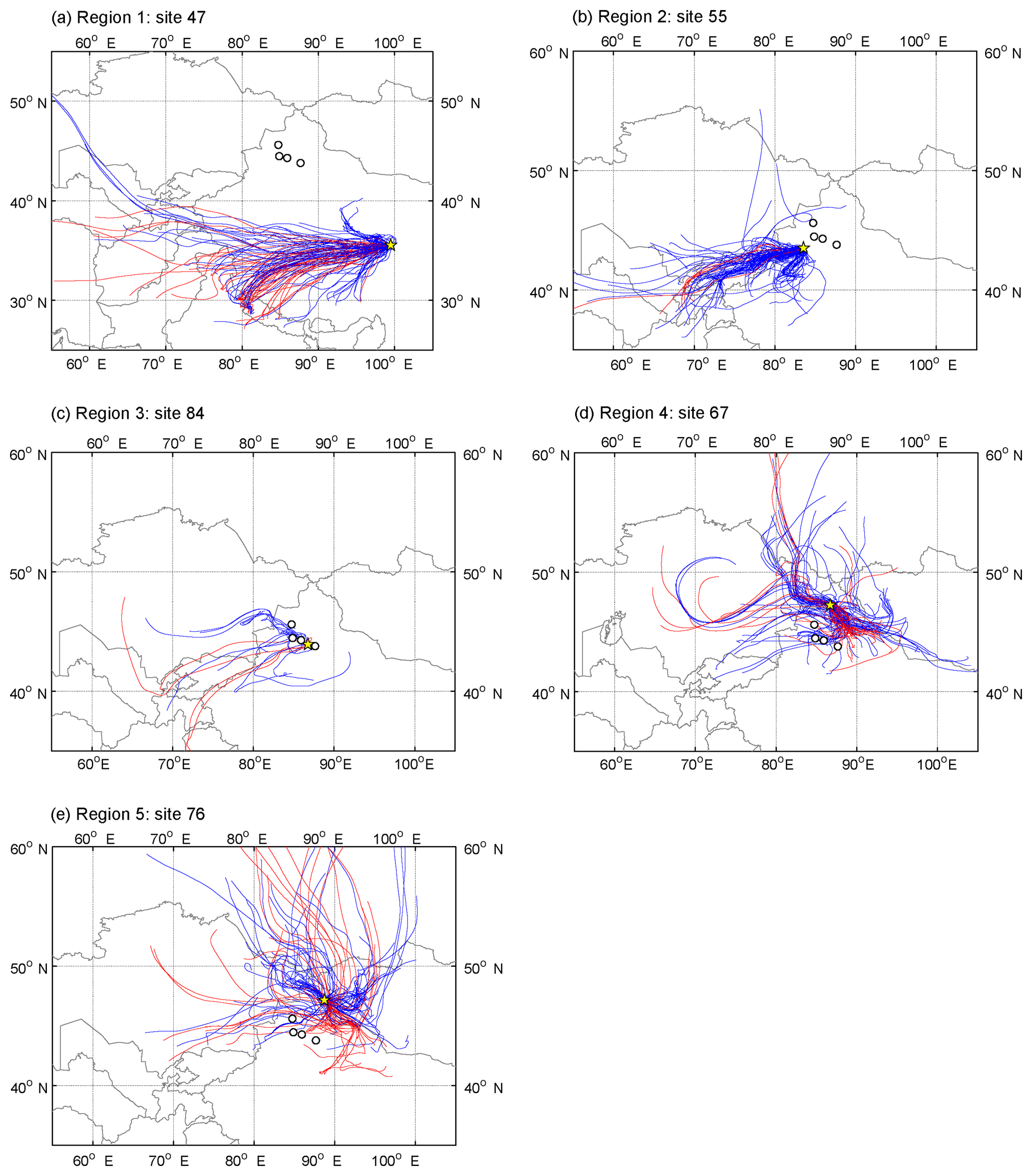
Figure 1072 h air mass backward trajectories at 500 m a.g.l. with the initial positions at representative sites (shown as yellow pentagrams) in each region. Trajectories were calculated 4 times per day for a period of 30 days preceding the sampling date at a given site by HYSPLIT (version 4, NOAA) except for panel (c). Since the snow was fresh at site 84, the trajectories were derived for 5 days preceding the sampling date. The red lines show the air masses that passed through the active fires before reaching the receptor sites, and the blue lines are those did not pass the fires. The white dots represent the typical industrial cities in Xinjiang, i.e., Karamay, Kuytun, Shihezi, and Urumqi from west to east.
In region 2, the contribution of soil dust to snow CDOM was also remarkable, which was proven by the high average %C1 and low average Fmax (C2)/Fmax (C1). Along the paths of the air masses to site 55 (Fig. 10b), very few trajectories encountered fires. Additionally, the average of (+)∕nss-ndust was also low, which showed the insignificant role of anthropogenic pollution. Therefore, in region 2, a major source of soil is found.
In region 3, the averages of Fmax (C2)/Fmax (C1) and (+)/nss-ndust were significantly higher than those in other regions (ANOVA, p<0.05), implying a strong influence of anthropogenic pollution. The mass ratio of Cl− and Na+ (2.48, Fig. S6) was approximately 2 times higher than that in seawater (1.18, Hara et al., 2004), which indicated that Cl− might originate from other sources in addition to sea salt such as coal combustion (Wang et al., 2008; Y. Wang et al., 2006), while the values in other regions were comparable to 1.18. This result again confirmed that the CDOM from pollution was dominant in region 3 but inapparent in other regions. The backward trajectories also showed consistent results (Fig. 10c). Most of the trajectories to site 84 came from the northwest and passed through the cities with heavy industry (e.g., Karamay and Shihezi). Therefore, air pollutants can be transported to the sample area and deposited on surface snow.
In regions 4 and 5, the nonsoil sources of snow CDOM were predominant due to the high regional averages of Fmax (C2)/Fmax (C1). In region 4, many of the air masses, which originated from central Asia (west), Siberia (north), and central Xinjiang (south), passed through the active fires and strongly influenced this region (Fig. 10d). The ratios of () and were significantly lower than those in region 3 (ANOVA, p<0.05), indicating a major source of biomass burning. Coincidentally, in region 5, the value of ()/ was comparable with that of region 4, which suggested CDOM from biomass burning rather than pollution. The respectable amount of air mass which encountered fires (Fig. 10e) can explain this finding. Furthermore, the low mass ratios of Cl− and Na+ in regions 4 and 5 also implied the slight influence of anthropogenic pollution. Overall, biomass burning is the dominant source both in regions 4 and 5.
Pu et al. (2017) used a positive matrix factorization (PMF) model to identify the sources of particulate light absorption of ILAPs (denoted as in snow during the same field campaign. The comparison of and aCDOM(280) among regions is shown in Fig. S7. In regions 1, 2, and 5, there was no significant correlation between and aCDOM(280), which indicated the entirely different sources of CDOM and particulate absorption of ILAPs. As reported by Pu et al. (2017), the major sources of were biomass burning in regions 1–2 and industrial pollution in region 5, while those of CDOM in this study were soil dust and biomass burning. Robust linear correlations were found in regions 3 and 4 (R2 is 0.95 and 0.75), which implied high consistency for sources of CDOM and particulate absorption of ILAPs (i.e., anthropogenic pollution and biomass burning, respectively).
3.4 Comparing the light absorption by CDOM and BC
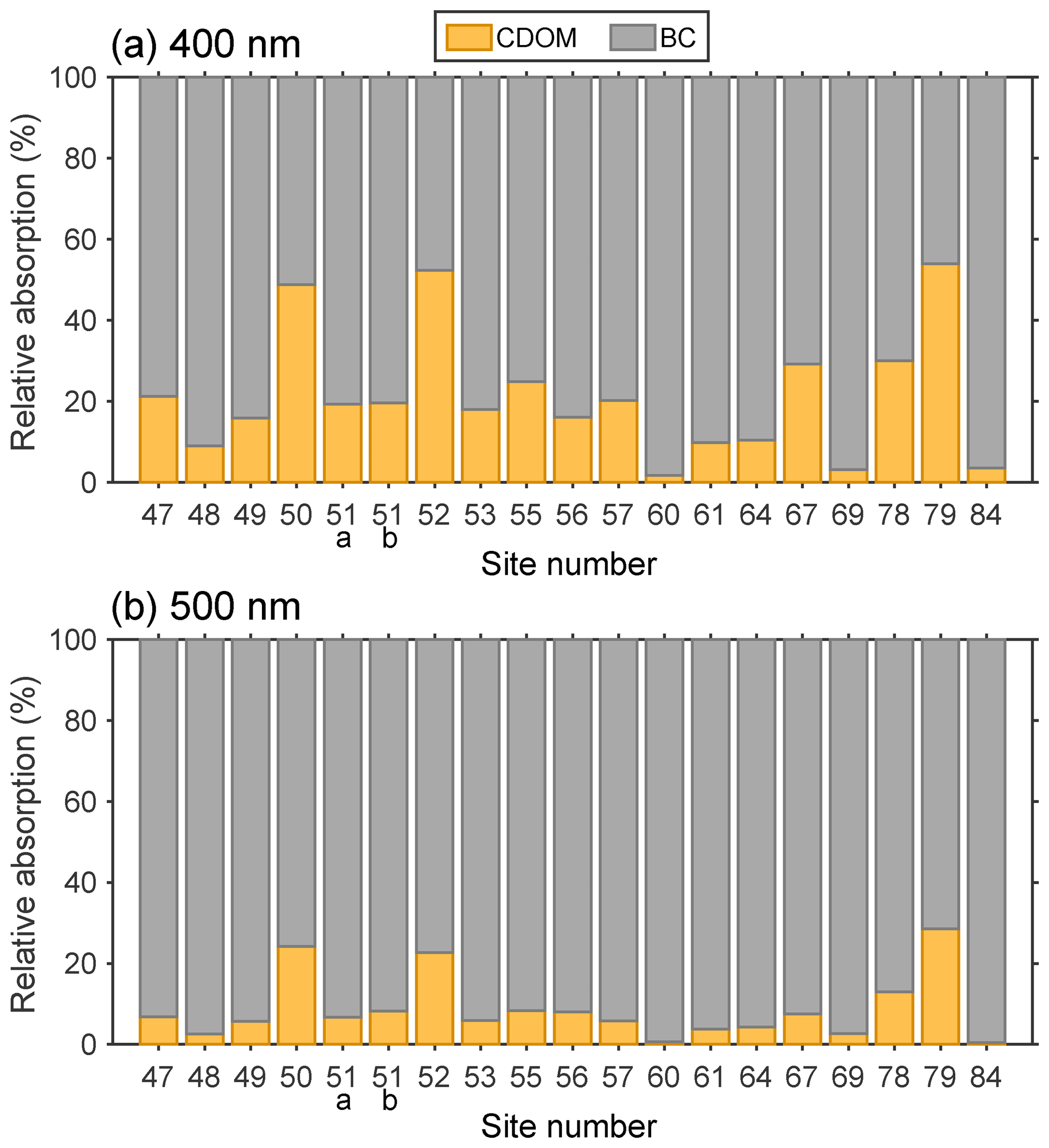
Figure 11 shows the relative contributions of CDOM and BC to light absorption. As mentioned above, light absorption within visible wavelengths was available for 19 samples. The BC concentrations in surface snow were obtained from Pu et al. (2017), and the MAC and AAE of BC used in the calculation were 6.3 m2 g−1 (550 nm) and 1.1 (Pu et al., 2017).
Most of these sites were assigned to cluster A, except sites 60, 69, and 84. As discussed in Sect. 3.2.2, sites of cluster A exhibited high values of %C1, indicating that CDOM mainly originated from soil dust. At sites 50, 52, and 79, the light absorptions of CDOM and BC were roughly equal at 400 nm. It was not only due to the high abundances of CDOM but also the relatively low BC mixing ratios in snow (approximately 30 ng g−1, Pu et al., 2017). Sites 60, 69, and 84, where the fluorescence intensities were dominated by C2, were the only three sites assigned to cluster C. Biomass burning and anthropogenic pollution (e.g., fossil fuel combustion) are both major sources of fluorophore C2 and BC. Therefore, the BC mixing ratios were approximately 300 ng g−1 at these sites (Pu et al., 2017), leading to quite low ratios of light absorption due to CDOM and BC (approximately 0.03 at 400 nm). At other sites, this value was typically in the range of 0.1 to 0.4. In summary, the light absorption of CDOM was 0.34±0.34 times that for BC at 400 nm. At 500 nm, this value decreased quickly to 0.10±0.11 due to the stronger wavelength dependence of CDOM absorption. This finding is quite different from the results for snow samples collected at Barrow, Alaska. As presented by Doherty et al. (2013), the mixing ratio of BC in Barrow snow ranged between 10 and 30 ng g−1; however, the equivalent BC mixing ratio of CDOM absorption was only 0.14 ng g−1 at 400 nm and 0.07 ng g−1 at 550 nm (Dang and Hegg, 2014). Hence, the absorption of CDOM in Alaskan snow can be safely ignored, but this does not appear reasonable for some areas across northwestern China.
Previous studies have focused on the insoluble particles (e.g., BC, ISOC, and MD) in seasonal snow (Doherty et al., 2010, 2014; Pu et al., 2017; Wang et al., 2013). The above discussion indicates that in some specific areas of northwestern China, the absorption of CDOM in snow was remarkable. In addition to the results of cluster analysis, we summarized several absorption- and fluorescence-related indices of these sites. The average S275−295 (0.0187±0.0022) of these 19 sites was lowest compared to those of regions 1–5. The averages of BIX (0.60±0.20), FI (1.31±0.09), and Fmax (C2)/Fmax (C1) (1.66±1.03) were lower than those of region 2, in which the influence of local soil dust was obvious. Besides, the averages of HIX (1.87±0.57) and %C1 (30 %) were higher than those of region 2. These results confirmed that the CDOM of these sites was undoubtedly from terrestrial origins (e.g., wind-blown soil dust). Hence, we suggest that the absorption by CDOM in the snowpack, which is heavily affected by soil, cannot be ignored.
Seasonal snow samples were collected across northwestern China from January to February 2012. The aCDOM(280) and S275−295 of snow CDOM ranged from 0.15 to 10.57 m−1 and 0.0129 to 0.0389 nm−1. The average value of aCDOM(280) (1.69±1.80 m−1) was approximately 10 times higher than that in Alaska (Beine et al., 2011). Samples in Qinghai (region 1) exhibited the highest average aCDOM(280) (2.30±0.52 m−1) and the lowest average S275−295 (0.0188±0.0015 nm−1), resulting from the strong influence of local soil dust. Lower average aCDOM(280) appeared in central Xinjiang (region 3, 0.93±0.68 m−1), where almost all the samples were collected from new-fallen snow, and northwestern Xinjiang (region 4, 0.80±0.62 m−1 when excluding site 67), which was far from industrial areas. In the Tianshan Mountains (region 2) and northeastern Xinjiang (region 5), the average values of aCDOM(280) were 2.00±1.50 m−1 and 1.17±0.63 m−1. For all sites in Qinghai and some sites in Xinjiang (19 of 39 sites), the light absorption of CDOM cannot be neglected and was even remarkable (0.34±0.34 times relative to BC at 400 nm) due to the high contribution of CDOM from soil dust. Hence, we suggest that the CDOM absorption in visible wavelengths at such sites should be taken into consideration in future studies.
Based on PARAFAC analysis, two humic-like fluorophores (C1 and C2) and one protein-like fluorophore (C3) were identified. In Qinghai, %C1 (35 % on average) was much higher than those of the other regions; besides, the highest HIX, the lowest BIX and FI were also found. In Xinjiang (regions 2–5), %C1 varied among the regions. In region 2, C1 accounted for approximately 25 % to the total fluorescence, followed by regions 4 and 5 (both 17 % on average). In region 3, C1 contribution was the lowest (9 % on average), and the values of fluorescence-derived indices also showed consistent results (the lowest HIX, the highest BIX and FI). A hierarchical cluster analysis was used to classify samples into four clusters (A–D) based on the relative intensities of three fluorescent components. All samples in region 1 and most samples in region 2 were assigned to cluster A (a high contribution of C1). The number of samples assigned to cluster B (roughly equal contributions of C2 and C3) and cluster C (a dominant contribution of C2) were nearly even in region 3. For regions 4 and 5, most samples were classified into cluster B. Only two samples were assigned to cluster D due to the dominant contribution of C3.
According to the correlation analysis between Fmax (C2) and three major ions (, , and , as well as the mutual relationships among three fluorescent components, C2 exhibited potential sources of soil dust, microbial activity, anthropogenic pollution, and biomass burning. Furthermore, the regional distribution of CDOM sources was assessed by using variations of Fmax (C2)/Fmax (C1), ()/, , and air mass backward trajectory analysis. The major sources were soil dust for regions 1–2, anthropogenic pollution for region 3, and biomass burning for regions 4–5.
This study investigated the optical characteristics and potential sources of CDOM in seasonal snow across northwestern China. Future studies should focus on the molecular characteristics of snow CDOM and the relationship with optical properties, which is of great importance to the energy budget of snowpack and the global carbon cycle.
All data sets and codes used to produce this study can be obtained by contacting Xin Wang (wxin@lzu.edu.cn). The elevation data used in this study are available at: https://rda.ucar.edu/datasets/ds759.3/description (last access: 10 January 2019, National Geophysical Data Center/NESDIS/NOAA/U.S. Department of Commerce, 2001).
The supplement related to this article is available online at: https://doi.org/10.5194/tc-13-157-2019-supplement.
YZ drew the figures and wrote the manuscript. HW and YZ analyzed the data of light absorption, fluorescence, and ions, and also performed the backward trajectory analysis. JL, WP, and XW conducted the experiments. QC conducted the PARAFAC analysis. XW and YZ designed the experiments. All authors discussed and edited the manuscript.
The authors declare that they have no conflict of interest.
This research was supported by the Foundation for Innovative Research Groups
of the National Natural Science Foundation of China (41521004), the National
Natural Science Foundation of China (41522505, 41775144, 41877354, and 41703102), and the
Fundamental Research Funds for the Central Universities (lzujbky-2018-k02).
We thank Jinsen Shi of Lanzhou University, Hao Ye of Texas A&M
University, and Rudong Zhang of Nanjing University for their assistance in
field sampling. We thank Jiecan Cui of Lanzhou University and Yubin Zhou of
China National Deep Sea Center for their help in the revision of the
manuscript. We are grateful for the constructive comments from the editor
Florent Dominé and two anonymous referees.
Edited by: Florent Dominé
Reviewed by: two anonymous referees
Anastasio, C. and Robles, T.: Light absorption by soluble chemical species in Arctic and Antarctic snow, J. Geophys. Res.-Atmos., 112, D24304, https://doi.org/10.1029/2007JD008695, 2007.
Anesio, A. M., Hodson, A. J., Fritz, A., Psenner, R., and Sattler, B.: High microbial activity on glaciers: importance to the global carbon cycle, Glob. Change Biol., 15, 955–960, 2009.
Antony, R., Grannas, A. M., Willoughby, A. S., Sleighter, R. L., Thamban, M., and Hatcher, P. G.: Origin and Sources of Dissolved Organic Matter in Snow on the East Antarctic Ice Sheet, Environ. Sci. Technol., 48, 6151–6159, 2014.
Bahram, M., Bro, R., Stedmon, C., and Afkhami, A.: Handling of Rayleigh and Raman scatter for PARAFAC modeling of fluorescence data using interpolation, J. Chemometr., 20, 99–105, 2006.
Beine, H., Anastasio, C., Esposito, G., Patten, K., Wilkening, E., Domine, F., Voisin, D., Barret, M., Houdier, S., and Hall, S.: Soluble, light-absorbing species in snow at Barrow, Alaska, J. Geophys. Res.-Atmos., 116, D00R05, https://doi.org/10.1029/2011JD016181, 2011.
Bhatia, M. P., Das, S. B., Longnecker, K., Charette, M. A., and Kujawinski, E. B.: Molecular characterization of dissolved organic matter associated with the Greenland ice sheet, Geochim. Cosmochim. Ac., 74, 3768–3784, 2010.
Birdwell, J. E. and Engel, A. S.: Characterization of dissolved organic matter in cave and spring waters using UV-Vis absorbance and fluorescence spectroscopy, Org. Geochem., 41, 270–280, 2010.
Birdwell, J. E. and Valsaraj, K. T.: Characterization of dissolved organic matter in fogwater by excitation-emission matrix fluorescence spectroscopy, Atmos. Environ., 44, 3246–3253, 2010.
Bond, T. C.: Spectral dependence of visible light absorption by carbonaceous particles emitted from coal combustion, Geophys. Res. Lett., 28, 4075–4078, 2001.
Bricaud, A., Morel, A., and Prieur, L.: Absorption by dissolved Organic-matter of the sea (yellow substance) in the uv and visible domains, Limnol. Oceanogr., 26, 43–53, 1981.
Bro, R.: PARAFAC, Tutorial and applications, Chemometr. Intell. Lab., 38, 149–171, 1997.
Chen, Q. C., Miyazaki, Y., Kawamura, K., Matsumoto, K., Coburn, S., Volkamer, R., Iwamoto, Y., Kagami, S., Deng, Y. G., Ogawa, S., Ramasamy, S., Kato, S., Ida, A., Kajii, Y., and Mochida, M.: Characterization of Chromophoric Water-Soluble Organic Matter in Urban, Forest, and Marine Aerosols by HR-ToF-AMS Analysis and Excitation Emission Matrix Spectroscopy, Environ. Sci. Technol., 50, 10351–10360, 2016.
Coble, P. G.: Characterization of marine and terrestrial DOM in seawater using excitation emission matrix spectroscopy, Mar. Chem., 51, 325–346, 1996.
Coble, P. G., Del Castillo, C. E., and Avril, B.: Distribution and optical properties of CDOM in the Arabian Sea during the 1995 Southwest Monsoon, Deep-Sea Res. Pt. II, 45, 2195–2223, 1998.
Dang, C. and Hegg, D. A.: Quantifying light absorption by organic carbon in Western North American snow by serial chemical extractions, J. Geophys. Res.-Atmos., 119, 10247–10261, https://doi.org/10.1002/2014JD022156, 2014.
Del Castillo, C. E. and Coble, P. G.: Seasonal variability of the colored dissolved organic matter during the 1994–95 NE and SW Monsoons in the Arabian Sea, Deep-Sea Res. Pt. II, 47, 1563–1579, 2000.
Doherty, S. J., Warren, S. G., Grenfell, T. C., Clarke, A. D., and Brandt, R. E.: Light-absorbing impurities in Arctic snow, Atmos. Chem. Phys., 10, 11647–11680, https://doi.org/10.5194/acp-10-11647-2010, 2010.
Doherty, S. J., Grenfell, T. C., Forsstrom, S., Hegg, D. L., Brandt, R. E., and Warren, S. G.: Observed vertical redistribution of black carbon and other insoluble light-absorbing particles in melting snow, J. Geophys. Res.-Atmos., 118, 5553–5569, 2013.
Doherty, S. J., Dang, C., Hegg, D. A., Zhang, R. D., and Warren, S. G.: Black carbon and other light-absorbing particles in snow of central North America, J. Geophys. Res.-Atmos., 119, 12807–12831, 2014.
Doherty, S. J., Steele, M., Rigor, I., and Warren, S. G.: Interannual variations of light-absorbing particles in snow on Arctic sea ice, J. Geophys. Res.-Atmos., 120, 11391–11400, 2015.
Domine, F., Bock, J., Voisin, D., and Donaldson, D. J.: Can We Model Snow Photochemistry? Problems with the Current Approaches, J. Phys. Chem. A, 117, 4733–4749, 2013.
Duarte, R. M. B. O., Pio, C. A., and Duarte, A. C.: Synchronous scan and excitation-emission matrix fluorescence spectroscopy of water-soluble organic compounds in atmospheric aerosols, J. Atmos. Chem., 48, 157–171, 2004.
Dubnick, A., Barker, J., Sharp, M., Wadham, J., Lis, G., Telling, J., Fitzsimons, S., and Jackson, M.: Characterization of dissolved organic matter (DOM) from glacial environments using total fluorescence spectroscopy and parallel factor analysis, Ann. Glaciol., 51, 111–122, 2010.
Fellman, J. B., D'Amore, D. V., and Hood, E.: An evaluation of freezing as a preservation technique for analyzing dissolved organic C, N and P in surface water samples, Sci. Total Environ., 392, 305–312, 2008.
Feng, L., Xu, J. Z., Kang, S. C., Li, X. F., Li, Y., Jiang, B., and Shi, Q.: Chemical Composition of Microbe-Derived Dissolved Organic Matter in Cryoconite in Tibetan Plateau Glaciers: Insights from Fourier Transform Ion Cyclotron Resonance Mass Spectrometry Analysis, Environ. Sci. Technol., 50, 13215–13223, 2016.
Feng, L., An, Y., Xu, J., Kang, S., Li, X., Zhou, Y., Zhang, Y., Jiang, B., and Liao, Y.: Physical and chemical evolution of dissolved organic matter across the ablation season on a glacier in the central Tibetan Plateau, Biogeosciences Discuss., https://doi.org/10.5194/bg-2017-507, 2017.
Fichot, C. G. and Benner, R.: The spectral slope coefficient of chromophoric dissolved organic matter (S275-295) as a tracer of terrigenous dissolved organic carbon in river-influenced ocean margins, Limnol. Oceanogr., 57, 1453–1466, 2012.
Graber, E. R. and Rudich, Y.: Atmospheric HULIS: How humic-like are they? A comprehensive and critical review, Atmos. Chem. Phys., 6, 729–753, https://doi.org/10.5194/acp-6-729-2006, 2006.
Hadley, O. L. and Kirchstetter, T. W.: Black-carbon reduction of snow albedo, Nat. Clim. Change, 2, 437–440, 2012.
Hansen, A. M., Kraus, T. E. C., Pellerin, B. A., Fleck, J. A., Downing, B. D., and Bergamaschi, B. A.: Optical properties of dissolved organic matter (DOM): Effects of biological and photolytic degradation, Limnol. Oceanogr., 61, 1015–1032, 2016.
Hara, K., Osada, K., Kido, M., Hayashi, M., Matsunaga, K., Iwasaka, Y., Yamanouchi, T., Hashida, G., and Fukatsu, T.: Chemistry of sea-salt particles and inorganic halogen species in Antarctic regions: Compositional differences between coastal and inland stations, J. Geophys. Res.-Atmos., 109, D20208, https://doi.org/10.1029/2004JD004713, 2004.
Hecobian, A., Zhang, X., Zheng, M., Frank, N., Edgerton, E. S., and Weber, R. J.: Water-Soluble Organic Aerosol material and the light-absorption characteristics of aqueous extracts measured over the Southeastern United States, Atmos. Chem. Phys., 10, 5965–5977, https://doi.org/10.5194/acp-10-5965-2010, 2010.
Hegg, D. A., Warren, S. G., Grenfell, T. C., Sarah J. Doherty, and Clarke, A. D.: Sources of light-absorbing aerosol in arctic snow and their seasonal variation, Atmos. Chem. Phys., 10, 10923–10938, https://doi.org/10.5194/acp-10-10923-2010, 2010.
Helms, J. R., Stubbins, A., Ritchie, J. D., Minor, E. C., Kieber, D. J., and Mopper, K.: Absorption spectral slopes and slope ratios as indicators of molecular weight, source, and photobleaching of chromophoric dissolved organic matter, Limnol. Oceanogr., 53, 955–969, 2008.
Helms, J. R., Stubbins, A., Perdue, E. M., Green, N. W., Chen, H., and Mopper, K.: Photochemical bleaching of oceanic dissolved organic matter and its effect on absorption spectral slope and fluorescence, Mar. Chem., 155, 81–91, 2013.
Hill, V. J. and Zimmerman, R. C.: Characteristics of colored dissolved organic material in first year landfast sea ice and the underlying water column in the Canadian Arctic in the early spring, Mar. Chem., 180, 1–13, 2016.
Hood, E., Fellman, J., Spencer, R. G. M., Hernes, P. J., Edwards, R., D'Amore, D., and Scott, D.: Glaciers as a source of ancient and labile organic matter to the marine environment, Nature, 462, 1044–1047, 2009.
Hood, E., Battin, T. J., Fellman, J., O'Neel, S., and Spencer, R. G. M.: Storage and release of organic carbon from glaciers and ice sheets, Nat. Geosci., 8, 91–96, 2015.
Huang, J. P., Fu, Q. A., Zhang, W., Wang, X., Zhang, R. D., Ye, H., and Warren, S. G.: Dust And Black Carbon In Seasonal Snow across Northern China, B. Am. Meteorol. Soc., 92, 175–181, 2011.
Huang, S. B., Wang, Y. X., Ma, T., Tong, L., Wang, Y. Y., Liu, C. R., and Zhao, L.: Linking groundwater dissolved organic matter to sedimentary organic matter from a fluvio-lacustrine aquifer at Jianghan Plain, China by EEM-PARAFAC and hydrochemical analyses, Sci. Total Environ., 529, 131–139, 2015.
Huguet, A., Vacher, L., Relexans, S., Saubusse, S., Froidefond, J. M., and Parlanti, E.: Properties of fluorescent dissolved organic matter in the Gironde Estuary, Org. Geochem., 40, 706–719, 2009.
IPCC: Climate Change 2013: The Physical Science Basis. Contribution of Working Group I to the Fifth Assessment Report of the Intergovernmental Panel on Climate Change, edited by: Stocker, T. F., Qin, D., Plattner, G.-K., Tignor, M., Allen, S. K., Boschung, J., Nauels, A., Xia, Y., Bex, V., and Midgley, P. M., Cambridge University Press, Cambridge, United Kingdom and New York, NY, USA, 1535 pp., 2013.
Jones, H. G.: The ecology of snow-covered systems: a brief overview of nutrient cycling and life in the cold, Hydrol. Process., 13, 2135–2147, 1999.
Kothawala, D. N., Murphy, K. R., Stedmon, C. A., Weyhenmeyer, G. A., and Tranvik, L. J.: Inner filter correction of dissolved organic matter fluorescence, Limnol. Oceanogr.-Meth., 11, 616–630, 2013.
Lawaetz, A. J. and Stedmon, C. A.: Fluorescence Intensity Calibration Using the Raman Scatter Peak of Water, Appl. Spectrosc., 63, 936–940, 2009.
Lawson, E. C., Wadham, J. L., Tranter, M., Stibal, M., Lis, G. P., Butler, C. E. H., Laybourn-Parry, J., Nienow, P., Chandler, D., and Dewsbury, P.: Greenland Ice Sheet exports labile organic carbon to the Arctic oceans, Biogeosciences, 11, 4015–4028, https://doi.org/10.5194/bg-11-4015-2014, 2014.
Lee, H. J., Laskin, A., Laskin, J., and Nizkorodov, S. A.: Excitation-Emission Spectra and Fluorescence Quantum Yields for Fresh and Aged Biogenic Secondary Organic Aerosols, Environ. Sci. Technol., 47, 5763–5770, 2013.
Liu, Y. Q., Yao, T. D., Jiao, N. Z., Kang, S. C., Xu, B. Q., Zeng, Y. H., Huang, S. J., and Liu, X. B.: Bacterial diversity in the snow over Tibetan Plateau Glaciers, Extremophiles, 13, 411–423, 2009.
Lutz, S., Anesio, A. M., Raiswell, R., Edwards, A., Newton, R. J., Gill, F., and Benning, L. G.: The biogeography of red snow microbiomes and their role in melting arctic glaciers, Nat. Commun., 7, 11968, https://doi.org/10.1038/ncomms11968, 2016.
Massicotte, P., Asmala, E., Stedmon, C., and Markager, S.: Global distribution of dissolved organic matter along the aquatic continuum: Across rivers, lakes and oceans, Sci. Total Environ., 609, 180–191, 2017.
McKnight, D. M., Boyer, E. W., Westerhoff, P. K., Doran, P. T., Kulbe, T., and Andersen, D. T.: Spectrofluorometric characterization of dissolved organic matter for indication of precursor organic material and aromaticity, Limnol. Oceanogr., 46, 38–48, 2001.
Mladenov, N., Alados-Arboledas, L., Olmo, F. J., Lyamani, H., Delgado, A., Molina, A., and Reche, I.: Applications of optical spectroscopy and stable isotope analyses to organic aerosol source discrimination in an urban area, Atmos. Environ., 45, 1960–1969, 2011.
Mladenov, N., Williams, M. W., Schmidt, S. K., and Cawley, K.: Atmospheric deposition as a source of carbon and nutrients to an alpine catchment of the Colorado Rocky Mountains, Biogeosciences, 9, 3337–3355, https://doi.org/10.5194/bg-9-3337-2012, 2012.
Murphy, K. R., Stedmon, C. A., Waite, T. D., and Ruiz, G. M.: Distinguishing between terrestrial and autochthonous organic matter sources in marine environments using fluorescence spectroscopy, Mar. Chem., 108, 40–58, 2008.
Murphy, K. R., Hambly, A., Singh, S., Henderson, R. K., Baker, A., Stuetz, R., and Khan, S. J.: Organic Matter Fluorescence in Municipal Water Recycling Schemes: Toward a Unified PARAFAC Model, Environ. Sci. Technol., 45, 2909–2916, 2011.
Murphy, K. R., Stedmon, C. A., Graeber, D., and Bro, R.: Fluorescence spectroscopy and multi-way techniques. PARAFAC, Anal. Methods-Uk., 5, 6557–6566, 2013.
MCD14DL: NASA Near Real-Time and MCD14DL MODIS Active Fire Detections, TXT format, Data set, available at: https://earthdata.nasa.gov/firms, last access: 2 October, 2018.
National Geophysical Data Center/NESDIS/NOAA/U.S. Department of Commerce: ETOPO2, Global 2 Arc-minute Ocean Depth and Land Elevation from the US National Geophysical Data Center (NGDC), Research Data Archive at the National Center for Atmospheric Research, Computational and Information Systems Laboratory, https://doi.org/10.5065/D6668B75, 2001.
Niu, H. W., Kang, S. C., Lu, X. X., and Shi, X. F.: Distributions and light absorption property of water soluble organic carbon in a typical temperate glacier, southeastern Tibetan Plateau, Tellus B, 70, 1445379, https://doi.org/10.1080/16000889.2018.1468705, 2018.
Oh, M. S., Lee, T. J., and Kim, D. S.: Quantitative Source Apportionment of Size-segregated Particulate Matter at Urbanized Local Site in Korea, Aerosol Air Qual. Res., 11, 247–264, 2011.
Otero, M., Mendonca, A., Valega, M., Santos, E. B. H., Pereira, E., Esteves, V. I., and Duarte, A.: Fluorescence and DOC contents of estuarine pore waters from colonized and non-colonized sediments: Effects of sampling preservation, Chemosphere, 67, 211–220, 2007.
Peacock, M., Freeman, C., Gauci, V., Lebron, I., and Evans, C. D.: Investigations of freezing and cold storage for the analysis of peatland dissolved organic carbon (DOC) and absorbance properties, Environ. Sci.-Proc. Imp., 17, 1290–1301, 2015.
Pegau, W. S.: Inherent optical properties of the central Arctic surface waters, J. Geophys. Res.-Oceans, 107, 8035, https://doi.org/10.1029/2000JC000382, 2002.
Pio, C. A., Legrand, M., Oliveira, T., Afonso, J., Santos, C., Caseiro, A., Fialho, P., Barata, F., Puxbaum, H., Sanchez-Ochoa, A., Kasper-Giebl, A., Gelencser, A., Preunkert, S., and Schock, M.: Climatology of aerosol composition (organic versus inorganic) at nonurban sites on a west-east transect across Europe, J. Geophys. Res.-Atmos., 112, D23S02, https://doi.org/10.1029/2006JD008038, 2007.
Pu, W., Wang, X., Wei, H., Zhou, Y., Shi, J., Hu, Z., Jin, H., and Chen, Q.: Properties of black carbon and other insoluble light-absorbing particles in seasonal snow of northwestern China, The Cryosphere, 11, 1213–1233, https://doi.org/10.5194/tc-11-1213-2017, 2017.
Saracli, S., Dogan, N., and Dogan, I.: Comparison of hierarchical cluster analysis methods by cophenetic correlation, J. Inequal. Appl., 203, 203, https://doi.org/10.1186/1029-242X-2013-203, 2013.
Seekell, D. A., Lapierre, J. F., Ask, J., Bergstrom, A. K., Deininger, A., Rodriguez, P., and Karlsson, J.: The influence of dissolved organic carbon on primary production in northern lakes, Limnol. Oceanogr., 60, 1276–1285, 2015.
Singer, G. A., Fasching, C., Wilhelm, L., Niggemann, J., Steier, P., Dittmar, T., and Battin, T. J.: Biogeochemically diverse organic matter in Alpine glaciers and its downstream fate, Nat. Geosci., 5, 710–714, 2012.
Spencer, R. G. M., Butler, K. D., and Aiken, G. R.: Dissolved organic carbon and chromophoric dissolved organic matter properties of rivers in the USA, J. Geophys. Res.-Biogeo., 117, G03001, https://doi.org/10.1029/2011JG001928, 2012.
Stedmon, C. A. and Bro, R.: Characterizing dissolved organic matter fluorescence with parallel factor analysis: a tutorial, Limnol. Oceanogr.-Meth., 6, 572–579, 2008.
Stedmon, C. A. and Markager, S.: Tracing the production and degradation of autochthonous fractions of dissolved organic matter by fluorescence analysis, Limnol. Oceanogr., 50, 1415–1426, 2005a.
Stedmon, C. A. and Markager, S.: Resolving the variability in dissolved organic matter fluorescence in a temperate estuary and its catchment using PARAFAC analysis, Limnol. Oceanogr., 50, 686–697, 2005b.
Stedmon, C. A., Markager, S., and Bro, R.: Tracing dissolved organic matter in aquatic environments using a new approach to fluorescence spectroscopy, Mar. Chem., 82, 239–254, 2003.
Stein, A. F., Draxler, R. R., Rolph, G. D., Stunder, B. J. B., Cohen, M. D., and Ngan, F.: Noaa's Hysplit Atmospheric Transport and Dispersion Modeling System, B. Am. Meteorol. Soc., 96, 2059–2077, 2015.
Stubbins, A., Hood, E., Raymond, P. A., Aiken, G. R., Sleighter, R. L., Hernes, P. J., Butman, D., Hatcher, P. G., Striegl, R. G., Schuster, P., Abdulla, H. A. N., Vermilyea, A. W., Scott, D. T., and Spencer, R. G. M.: Anthropogenic aerosols as a source of ancient dissolved organic matter in glaciers, Nat. Geosci., 5, 198–201, 2012.
Thieme, L., Graeber, D., Kaupenjohann, M., and Siemens, J.: Fast-freezing with liquid nitrogen preserves bulk dissolved organic matter concentrations, but not its composition, Biogeosciences, 13, 4697–4705, https://doi.org/10.5194/bg-13-4697-2016, 2016.
Thrane, J.-E., Hessen, D. O., and Andersen, T.: The Absorption of Light in Lakes: Negative Impact of Dissolved Organic Carbon on Primary Productivity, Ecosystems, 17, 1040–1052, 2014.
Twardowski, M. S., Boss, E., Sullivan, J. M., and Donaghay, P. L.: Modeling the spectral shape of absorption by chromophoric dissolved organic matter, Mar. Chem., 89, 69–88, 2004.
Vaehaetalo, A. V. and Wetzel, R. G.: Photochemical and microbial decomposition of chromophoric dissolved organic matter during long (months-years) exposures, Mar. Chem., 89, 313–326, 2004.
VNP14IMGTDL_NRT: NASA Near Real-Time VNP14IMGTDL_NRT VIIRS 375 m Active Fire Detections, TXT format, Data set, available at: https://earthdata.nasa.gov/firms, last access: 2 October, 2018.
Voisin, D., Jaffrezo, J. L., Houdier, S., Barret, M., Cozic, J., King, M. D., France, J. L., Reay, H. J., Grannas, A., Kos, G., Ariya, P. A., Beine, H. J., and Domine, F.: Carbonaceous species and humic like substances (HULIS) in Arctic snowpack during OASIS field campaign in Barrow, J. Geophys. Res.-Atmos., 117, D00R19, https://doi.org/10.1029/2011JD016612, 2012.
Wang, H. L., Zhuang, Y. H., Wang, Y., Sun, Y., Yuan, H., Zhuang, G. S., and Hao, Z. P.: Long-term monitoring and source apportionment of PM2.5/PM10 in Beijing, China, J. Environ. Sci.-China, 20, 1323–1327, 2008.
Wang, X., Doherty, S. J., and Huang, J.: Black carbon and other light-absorbing impurities in snow across Northern China, J. Geophys. Res.-Atmos., 118, 1471–1492, 2013.
Wang, X., Pu, W., Zhang, X. Y., Ren, Y., and Huang, J. P.: Water-soluble ions and trace elements in surface snow and their potential source regions across northeastern China, Atmos. Environ., 114, 57–65, 2015.
Wang, X., Pu, W., Ren, Y., Zhang, X., Zhang, X., Shi, J., Jin, H., Dai, M., and Chen, Q.: Observations and model simulations of snow albedo reduction in seasonal snow due to insoluble light-absorbing particles during 2014 Chinese survey, Atmos. Chem. Phys., 17, 2279–2296, https://doi.org/10.5194/acp-17-2279-2017, 2017.
Wang, Y., Zhuang, G. S., Zhang, X. Y., Huang, K., Xu, C., Tang, A. H., Chen, J. M., and An, Z. S.: The ion chemistry, seasonal cycle, and sources of PM2.5 and TSP aerosol in Shanghai, Atmos. Environ., 40, 2935–2952, 2006.
Wang, Y. H., Xu, Y. P., Spencer, R. G. M., Zito, P., Kellerman, A., Podgorski, D., Xiao, W. J., Wei, D. D., Rashid, H., and Yang, Y. H.: Selective Leaching of Dissolved Organic Matter From Alpine Permafrost Soils on the Qinghai-Tibetan Plateau, J. Geophys. Res.-Biogeo., 123, 1005–1016, 2018.
Warren, S. G. and Wiscombe, W. J.: A Model for the Spectral Albedo of Snow. 2.Snow Containing Atmospheric Aerosols, J. Atmos. Sci., 37, 2734–2745, 1980.
Xie, M. J., Mladenov, N., Williams, M. W., Neff, J. C., Wasswa, J., and Hannigan, M. P.: Water soluble organic aerosols in the Colorado Rocky Mountains, USA: composition, sources and optical properties, Sci. Rep.-Uk., 6, 39339, https://doi.org/10.1038/srep39339, 2016.
Yamashita, Y., Jaffe, R., Maie, N., and Tanoue, E.: Assessing the dynamics of dissolved organic matter (DOM) in coastal environments by excitation emission matrix fluorescence and parallel factor analysis (EEM-PARAFAC), Limnol. Oceanogr., 53, 1900–1908, 2008.
Yamashita, Y., Cory, R. M., Nishioka, J., Kuma, K., Tanoue, E., and Jaffe, R.: Fluorescence characteristics of dissolved organic matter in the deep waters of the Okhotsk Sea and the northwestern North Pacific Ocean, Deep-Sea Res. Pt. II, 57, 1478–1485, 2010.
Yan, F., Kang, S., Li, C., Zhang, Y., Qin, X., Li, Y., Zhang, X., Hu, Z., Chen, P., Li, X., Qu, B., and Sillanpää, M.: Concentration, sources and light absorption characteristics of dissolved organic carbon on a medium-sized valley glacier, northern Tibetan Plateau, The Cryosphere, 10, 2611–2621, https://doi.org/10.5194/tc-10-2611-2016, 2016.
Yang, L. Y., Hong, H. S., Chen, C. T. A., Guo, W. D., and Huang, T. H.: Chromophoric dissolved organic matter in the estuaries of populated and mountainous Taiwan, Mar. Chem., 157, 12–23, 2013.
Ye, H., Zhang, R. D., Shi, J. S., Huang, J. P., Warren, S. G., and Fu, Q.: Black carbon in seasonal snow across northern Xinjiang in northwestern China, Environ. Res. Lett., 7, 044002, https://doi.org/10.1088/1748-9326/7/4/044002, 2012.
Yu, H. R., Liang, H., Qu, F. S., Han, Z. S., Shao, S. L., Chang, H. Q., and Li, G. B.: Impact of dataset diversity on accuracy and sensitivity of parallel factor analysis model of dissolved organic matter fluorescence excitation-emission matrix, Sci. Rep.-Uk., 5, 10207, https://doi.org/10.1038/srep10207, 2015.
Zhang, R., Hegg, D. A., Huang, J., and Fu, Q.: Source attribution of insoluble light-absorbing particles in seasonal snow across northern China, Atmos. Chem. Phys., 13, 6091–6099, https://doi.org/10.5194/acp-13-6091-2013, 2013.
Zhang, Y. L., van Dijk, M. A., Liu, M. L., Zhu, G. W., and Qin, B. Q.: The contribution of phytoplankton degradation to chromophoric dissolved organic matter (CDOM) in eutrophic shallow lakes: Field and experimental evidence, Water Res., 43, 4685–4697, 2009.
Zhang, Y. L., Zhang, E. L., Yin, Y., van Dijk, M. A., Feng, L. Q., Shi, Z. Q., Liu, M. L., and Qin, B. Q.: Characteristics and sources of chromophoric dissolved organic matter in lakes of the Yungui Plateau, China, differing in trophic state and altitude, Limnol. Oceanogr., 55, 2645–2659, 2010.
Zhang, Y. L., Yin, Y., Feng, L. Q., Zhu, G. W., Shi, Z. Q., Liu, X. H., and Zhang, Y. Z.: Characterizing chromophoric dissolved organic matter in Lake Tianmuhu and its catchment basin using excitation-emission matrix fluorescence and parallel factor analysis, Water Res., 45, 5110–5122, 2011.
Zhao, Y., Song, K., Wen, Z., Li, L., Zang, S., Shao, T., Li, S., and Du, J.: Seasonal characterization of CDOM for lakes in semiarid regions of Northeast China using excitation-emission matrix fluorescence and parallel factor analysis (EEM-PARAFAC), Biogeosciences, 13, 1635–1645, https://doi.org/10.5194/bg-13-1635-2016, 2016.
Zhou, Y., Wang, X., Wu, X., Cong, Z., Wu, G., and Ji, M.: Quantifying Light Absorption of Iron Oxides and Carbonaceous Aerosol in Seasonal Snow across Northern China, Atmosphere, 8, 63, https://doi.org/10.3390/atmos8040063, 2017.
Zhou, Y. Q., Yao, X. L., Zhang, Y. B., Shi, K., Zhang, Y. L., Jeppesen, E., Gao, G., Zhu, G. W., and Qin, B. Q.: Potential rainfall-intensity and pH-driven shifts in the apparent fluorescent composition of dissolved organic matter in rainwater, Environ. Pollut., 224, 638–648, 2017.
Zsolnay, A., Baigar, E., Jimenez, M., Steinweg, B., and Saccomandi, F.: Differentiating with fluorescence spectroscopy the sources of dissolved organic matter in soils subjected to drying, Chemosphere, 38, 45–50, 1999.