the Creative Commons Attribution 4.0 License.
the Creative Commons Attribution 4.0 License.
 | 12 Jun 2019
Seasonal components of freshwater runoff in Glacier Bay, Alaska: diverse spatial patterns and temporal change
David F. Hill
Jordan P. Beamer
Elizabeth R. Holzenthal
A high spatial resolution (250 m), distributed snow evolution and ablation model, SnowModel, is used to estimate current and future scenario freshwater runoff into Glacier Bay, Alaska, a fjord estuary that makes up part of Glacier Bay National Park and Preserve. The watersheds of Glacier Bay contain significant glacier cover (tidewater and land-terminating) and strong spatial gradients in topography, land cover, and precipitation. The physical complexity and variability of the region produce a variety of hydrological regimes, including rainfall-, snowmelt-, and ice-melt-dominated responses. The purpose of this study is to characterize the recent historical components of freshwater runoff to Glacier Bay and quantify the potential hydrological changes that accompany the worst-case climate scenario during the final decades of the 21st century. The historical (1979–2015) mean annual runoff into Glacier Bay is found to be 24.5 km3 yr−1, or equivalent to a specific runoff of 3.1 m yr−1, with a peak in July, due to the overall dominance of snowmelt processes that are largely supplemented by ice melt. Future scenarios (2070–2099) of climate and glacier cover are used to estimate changes in the hydrologic response of Glacier Bay. Under the representative concentration pathway (RCP) 8.5, the mean of five climate models produces a mean annual runoff of 27.5 km3 yr−1, 3.5 m yr−1, representing a 13 % increase from historical conditions. When spatially aggregated over the entire bay region, the projection scenario seasonal hydrograph is flatter, with weaker summer flows and higher winter flows. The peak flows shift to late summer and early fall, and rain runoff becomes the dominant overall process. The timing and magnitudes of modeled historical runoff are supported by a freshwater content analysis from a 24-year oceanographic conductivity–temperature–depth (CTD) dataset from the U.S. National Park Service's Southeast Alaska Inventory and Monitoring Network (SEAN). The hydrographs of individual watersheds display a diversity of changes between the historical period and projection scenario simulations, depending upon total glacier coverage, elevation distribution, landscape characteristics, and seasonal changes to the freezing line altitude.


South-central and southeastern Alaska (Fig. 1a) are regions of physical, climatological, and hydrological extremes. Precipitation rates in excess of 8 m yr−1 water equivalent (w.e.; Beamer et al., 2016) fall on high mountain ranges (4000–6000 m) in close proximity to the ocean. The steep terrain drives strong orographic gradients in precipitation and creates compact drainage networks that rapidly deliver runoff to the coastline. Due to significant snowfall fractions for much of the year, and considerable glacier cover, the runoff to the coastline has significant contributions from rainfall, snowmelt, and ice melt constituents. Glaciers cover 17 % (Beamer et al., 2016) of the Gulf of Alaska (GOA) watershed, and Neal et al. (2010) estimate that roughly half of the coastal runoff comes from glacier surfaces (ice melt, snowmelt, and direct rainfall on glacier surfaces). The volume of water that is delivered to the coast is noteworthy. The GOA watershed, with an area of 420 300 km2, has a runoff of approximately 760 km3 yr−1 and a specific runoff of 1.8 m yr−1 (Beamer et al., 2016). In contrast, the Mississippi River watershed has a runoff of approximately 610 km3 yr−1 and a specific runoff of 0.19 m yr−1 (Dai et al., 2009). This runoff to the GOA is one of the important physical drivers of Alaska's nearshore oceanography and contributes to the Alaska Coastal Current (ACC; Weingartner et al., 2005), water column stratification (Carmack, 2007), and a variety of economically important fisheries (Fissel et al., 2014).
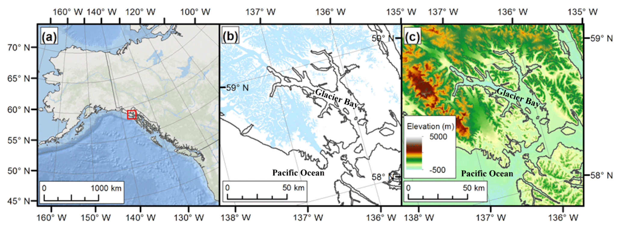
Figure 1Study area map. (a) Overview of the northern Gulf of Alaska; red box shows extent of panels (b) and (c). (b) Glacier cover (blue) in the Glacier Bay region from the Randolph Glacier Inventory (RGI; Pfeffer et al., 2014). (c) Bathymetry and elevation in the Glacier Bay region from the Southern Alaska Coastal Relief Model (Lim et al., 2011).
The hydrology of the GOA watershed is characterized by large seasonal variations in inputs (precipitation), outputs (runoff, evapotranspiration), and storage of water. Gravity Recovery and Climate Experiment (GRACE) satellite regional water storage data, for the period 2004–2013, show a mean annual accumulation of 295 km3 yr−1 and a mean annual ablation of 355 km3 yr−1 (Luthcke et al., 2013; Beamer et al., 2016) in the GOA watershed. The net decrease in regional water storage of 60 km3 yr−1 indicates that the region is also undergoing remarkable change. Indeed, the coastal mountain ranges of Alaska have recently sustained rapid rates of deglaciation (Arendt et al., 2002, 2009; Gardner et al., 2013; O'Neel et al., 2015). The mass loss from the glaciers within the GOA region, derived from airborne altimetry, is 64±10 km3 yr−1 (Larsen et al., 2015), which agrees well with the GRACE observations. Glacier volume loss (GVL) is a change in long-term water storage in a glacierized watershed and represents an additional flux of water that would not be present if the glacier system was in equilibrium with its environment (Radić and Hock, 2010). These additional fluxes can affect the physical and chemical oceanography in coastal Alaska's bays and fjords (Reisdorph and Mathis, 2014).
Glacier cover changes in response to long-term changes in meteorological forcing, and Beamer et al. (2017) have estimated future hydrographs for the GOA in response to changes in precipitation, temperature, and glacier cover. They consider a variety of climate model outputs and representative concentration pathways (RCPs). For RCP 8.5, which corresponds to a scenario of comparatively high greenhouse gas concentrations in the atmosphere, they find the overall runoff increases by 14 %, but the runoff from glacier surfaces decreases by about 34 %. Beamer et al. (2017) also find significant changes in the timing of the delivery of freshwater to the coast. In response to changes in temperature, precipitation, and glacier cover, summer flows are dramatically reduced, with strong increases in autumn and winter flows. The annual GOA hydrograph is estimated to change from a hydrograph dominated by a single summer peak to an annual hydrograph with two peaks: one due to spring snowmelt and the other due to autumn rains.
Glacier Bay (Fig. 1b–c) is a fjord estuary in southeast Alaska that makes up part of Glacier Bay National Park and Preserve (GBNPP). The bay itself is roughly Y-shaped, with maximum depths of approximately 500 m in the upper west and east arms and an overall volume of 162 km3. In contrast, depths near the entrance sill are approximately 25 m. The tidal forcing of the bay is considerable, with a great diurnal range (GT; difference between mean higher high water and mean lower low water) of 3.36 m (data from NOAA Station 9452634; Elfin Bay, AK). The large tidal range produces strong tidal mixing that tends to de-stratify the water column. This effect counteracts the large freshwater input to the bay that tends to stabilize the water column. The result is a complex pattern of spatial and temporal variability of water column properties. Etherington et al. (2007, their Fig. 5) summarize 10 years of oceanographic measurements (conductivity–temperature–depth (CTD) casts) made in Glacier Bay at a total of 24 stations (Fig. 2a). They aggregate the CTD measurements by month and by region (West Arm, East Arm, Central Bay, and Lower Bay). The results show that stratification is largest in the summer, due to the large runoff associated with ice melt. Spatially, a strong up-bay gradient in stratification exists, with the weakest stratification found in the Lower Bay, where shallow depths produced the strongest vertical mixing of the water column.
Etherington et al. (2007) correlate various water column properties (stratification, chlorophyll a, etc.) against physical variables such as day length, wind speed, and air temperature in order to develop a better understanding of the ecology of the bay. While their discussion considers the role played by freshwater inputs, the lack of observational data (stream gaging) and hydrological modeling studies of Glacier Bay leaves their hypotheses untested. Hill et al. (2009) apply the regression equations for flow exceedances (e.g., the discharge exceeded 50 % of the time) and peak flows (e.g., the 10-year event) developed by the USGS (Curran et al., 2003; Wiley and Curran, 2003) to Glacier Bay in order to help constrain the likely range of flows into the Bay. Their results suggest that the 10-year return interval discharge into the bay is approximately 10 000 m3 s−1 and that the 50 % exceedance annual discharge is approximately 800 m3 s−1; however their study includes a different contributing area, with watersheds on the southern side of Icy Strait included.
As was the case with the GOA watershed as a whole, Glacier Bay is a region that continues to undergo dramatic change. Glaciers have retreated over 100 km since the end of the little ice age (LIA; Hall and Benson, 1995), and the volume of ice lost in the Glacier Bay region alone is enough to raise global sea levels by 0.8 cm (Larsen et al., 2005). This glacial retreat has led to rapid vegetation succession (Chapin et al., 1994) and to rapid uplift rates from isostatic rebound (30 mm yr−1; Larsen et al., 2005) that produce falling relative sea levels. The GRACE data for the Glacier Bay region show a downward trend of 12 cm yr−1 w.e., which is very close to the average decrease of 13.3 cm yr−1 obtained for the entire GOA watershed (Luthcke et al., 2013; Beamer et al., 2016).
Long-term shifts in terrestrial freshwater storage and runoff can have significant implications for oceanographic stratification and circulation that moderate biogeochemical and ecological activity within Glacier Bay. Since Glacier Bay is a highly understudied, relatively remote national park, the complete freshwater budget for the bay cannot be quantified due to the lack of available data. However, seasonal trends in modeled freshwater runoff can be qualitatively compared with seasonal trends in broadscale oceanographic salinity records. Etherington et al. (2007) find positive correlations between phytoplankton biomass and stratification levels in Glacier Bay. The competing forces of macro-tidal flushing and strong stratification within the glacially carved estuary generate temporally and spatially shifting trends in upwelling and nutrient availability (Etherington et al., 2007). Thus, accurate estimation of projection scenario runoff into Glacier Bay plays a paramount role in constraining future changes in water and nutrient circulation.
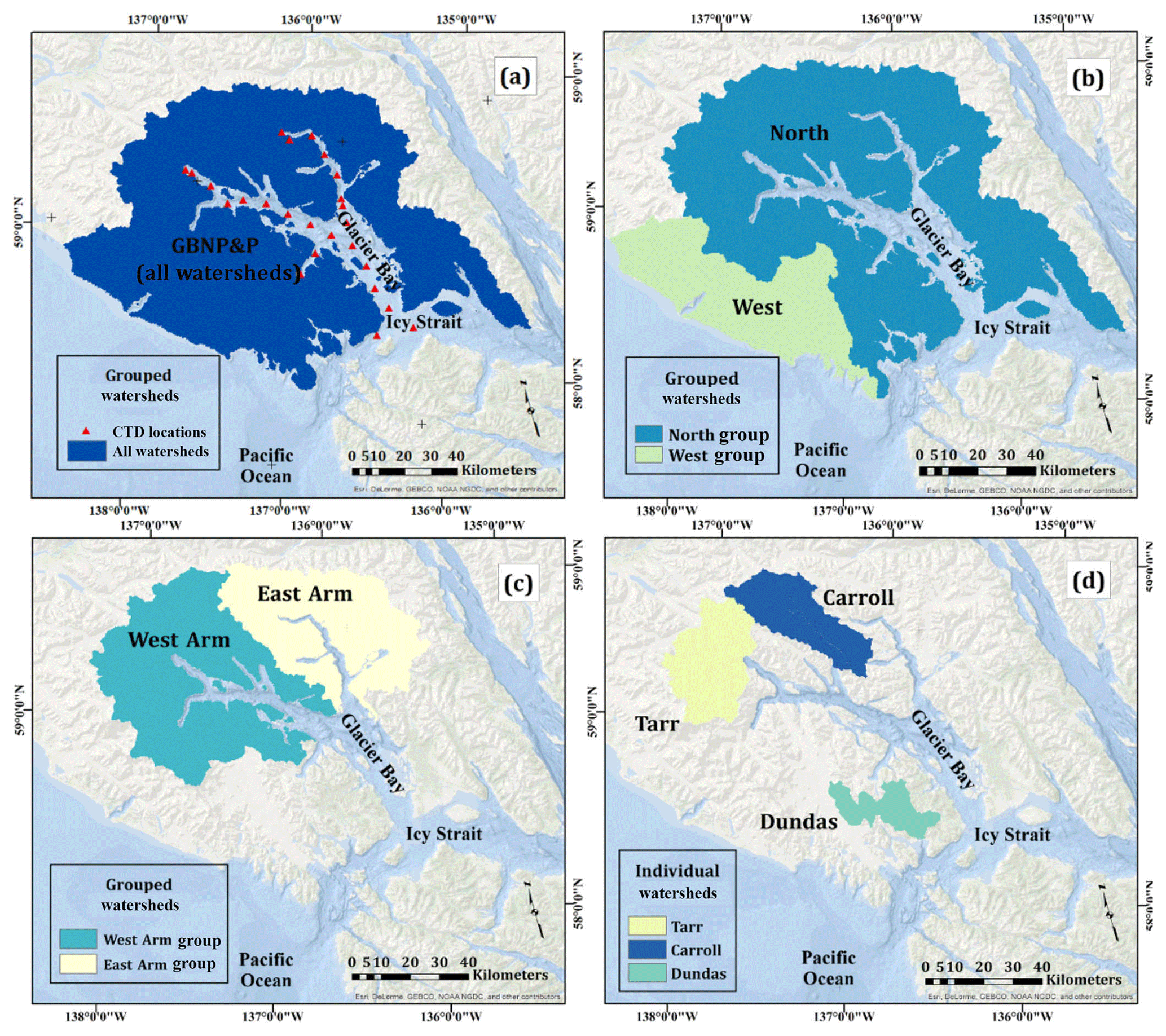
Figure 2Watershed maps. (a) All watersheds in the GBNPP group and the locations of the CTD casts (discussed in Sect. 3.3). (b) North and West grouped watersheds. The North delivers freshwater to the main stem of Glacier Bay, and the West delivers water to the Pacific Ocean. (c) The upper-bay grouped watersheds that deliver freshwater to the East Arm and West Arm of Glacier Bay. (d) The three individual watersheds: Tarr, Carroll, and Dundas.
This paper presents the results of a hydrological modeling study of Glacier Bay. We understand it to be the first high-resolution (sub-km), process-based study of the water cycle in the region. Recall that the results of Hill et al. (2009) are statistical and only provided a few representative flow values. Here, the goals are very different. We use an energy-balance model to evolve the snowpack and melt glacier ice after the seasonal snowpack disappears. Also, our model results are output on a 3-hourly time step, aggregated to daily, and then used to provide a variety of derived products (monthly averages, seasonal and annual climatologies, etc.). Glacier Bay is a high-gradient landscape (rapid spatial changes in terrain, precipitation, e.g.), and we anticipate considerable spatial variability in both present hydrographs as well as projection scenario hydrographs. The results of this study are used to characterize historical and projection scenario climatologies of runoff and thereby quantify seasonal changes in the delivery of freshwater to Glacier Bay. Using the observational U.S. National Park Service's Southeast Alaska Inventory and Monitoring Network (SEAN; discussed in Sect. 3.3) dataset allows the historical freshwater analysis of Glacier Bay to be contextualized. These results will add to the understanding developed by Etherington et al. (2007) and will provide constrained estimates of potential changes in runoff in GBNPP under the projection scenario.
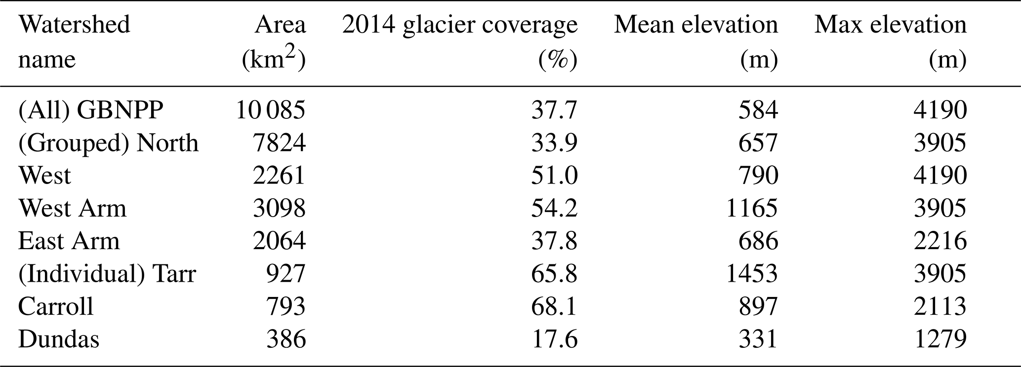
The study area lies mostly within the boundary of Glacier Bay National Park and Preserve and includes the many watersheds that flow to Glacier Bay, as well as watersheds along the Pacific coast south of the Alsek River. The aggregated watersheds in the study area (GBNPP) include some watersheds that originate outside the national park boundary, and are located partially in Canada. These watersheds are included in the analysis because the international boundary in this region resembles a straight line, fragmenting the natural watershed boundaries. The elevation in GBNPP ranges from sea level to heights in excess of 4500 m on Mt. Fairweather. The study area is divided into nested hydrologic units, which include three individual watersheds, four grouped watersheds, and the fully aggregated GBNPP model domain. These various domains are selected to illustrate the gradients in hydrologic inputs and outputs that exist in the region. See Table 1 and the following paragraph for more details about the spatial extent, average elevations, and glacier coverage of each grouped and individual watershed.
Table 1Key physical characteristics of the 8 sub-watersheds in the study area.
Within the GBNPP study area, there are four grouped watersheds. The northern group of watersheds (North; Fig. 2b) supplies freshwater to the mouth of Glacier Bay and constitutes the largest subgroup in the study area (see Table 1). The western group of watersheds (West; Fig. 2b) delivers freshwater to the Pacific Ocean directly. We further subdivide a portion of the North watershed into two smaller aggregated regions near the western (West Arm; Fig. 2c) and eastern (East Arm; Fig. 2c) regions of Glacier Bay. The two arms of Glacier Bay have notable differences in elevation, glacier cover, and water column properties, and the aggregated watersheds shown in Fig. 2c correspond to similar regions investigated by Etherington et al. (2007) and a large portion of the domain from Hill et al. (2009).
Finally, we examine several individual watersheds within GBNPP. The first is a small group of watersheds that includes the Margerie and Grand Pacific tidewater glaciers terminating in the Tarr Inlet in the West Arm of Glacier Bay (Tarr; Fig. 2d). The second is a highly glacierized region that includes Carroll Glacier, a land-terminating glacier with outlet lobes that deliver freshwater to the East Arm and West Arm of Glacier Bay (Carroll; Fig. 2d). The last is a low-elevation, rain-dominated watershed in the Dundas River region that experiences occasional glacial-lake outburst floods from the adjacent Brady Icefield (Dundas; Fig. 2d). We choose these three individual watersheds to illustrate and examine the various ice-melt-, snowmelt-, and rainfall-dominated runoff patterns and the changes they may experience in the projection scenario. The results of this study are categorized into the eight watersheds mentioned above. However, the focus of the results is on the aggregated GBNPP domain, and the appendices contain the supplemental grouped and individual watershed results.
3.1 Models
In this study we use a set of models to simulate freshwater runoff to Glacier Bay for two climatological periods: 1979–2015 and 2070–2099. First, MicroMet (Liston and Elder, 2006a) is used to distribute the gridded reanalysis forcing data throughout the model domain. Second, SnowModel (Liston and Elder, 2006b) is used to evolve the snowpack and melt glacier ice using energy-balance methods. This set of models is widely used in high-latitude, highly glacierized environments including Alaska (Beamer et al., 2016, 2017), the Arctic (Mernild et al., 2011; Liston and Hiemstra, 2011; Liston and Mernild, 2012; Mernild and Liston, 2012; Mernild et al., 2013, 2014), and the Andes (Mernild et al., 2017a–d). Below we only briefly review the model components. Readers are directed to the source publications for full details on model algorithms and to Beamer et al. (2016) for full details on the application of SnowModel to the GOA.
MicroMet (Liston and Elder, 2006a) is a meteorological distribution system for weather forcing datasets in high spatial resolution, distributed terrestrial modeling applications. The model relies upon the Barnes objective analysis scheme (Barnes, 1964, 1973) for spatial interpolation of atmospheric variables, generating data fields at each time step and grid cell in the model domain for eight atmospheric variables. The atmospheric variables required by MicroMet include surface level precipitation, wind speed and direction, relative humidity, and air temperature. Sub-models of MicroMet will calculate radiation fluxes if they are not available as inputs. Land cover and elevation datasets are also employed by MicroMet to establish relationships based on topographically and seasonally varying temperature lapse rates and topography-dependent wind and solar radiation fields.
SnowModel (Liston and Elder, 2006b) is a physically based model for estimating snowpack accumulation and ablation processes in snowy environments. Sub-models within SnowModel estimate the energy fluxes of the snowpack and generate the snow depths and snow water equivalence (SWE) for each cell in the gridded domain. The primary input for SnowModel is the gridded forcing dataset of atmospheric conditions that vary throughout the simulation time period and are distributed throughout the model domain by MicroMet. SnowModel does have the ability to melt glacier ice after the annual snowpack has fully melted away, but it does not include dynamic adjustments to the glacier cover volumes or extent. Therefore, SnowModel is able to simulate the hydrologic response of a fixed landscape, but it cannot simulate century-scale evolution of glacier cover. For this study, the time step of SnowModel is 3-hourly, and the results are aggregated to produce the monthly historical and projection scenario climatologies.
Water fluxes for all watersheds are given in terms of depths (m) rather than volumes (km3). This normalization by watershed area enables straightforward comparison between individual and grouped watersheds. Ice melt is runoff generated when glacial ice is melted after the seasonal snow disappears in each glacier grid cell. This definition of ice melt, as a runoff component, does not necessarily represent glacier volume loss, due again to the fact that SnowModel does not dynamically change glacier extent or volumes. These runoff component values for a watershed of interest are calculated by aggregating the values for all model grid cells in each watershed. Unlike the work of Beamer et al. (2016, 2017) we do not route the runoff across the landscape to the coastline. In GBNPP, the average distance from a grid cell to its coastal outlet is 9.0 km. Given this short distance, and the fact that our interest here is in seasonal climatologies of runoff, and not daily time series, this is a justifiable simplification.
3.2 Model forcing data
3.2.1 Elevation and land cover
The land surface elevation dataset is the National Aeronautics and Space Administration's (NASA) Shuttle Radar Topography Mission (SRTM; Farr et al., 2007) 90 m digital elevation model (DEM) resampled to 250 m. A model grid resolution of 250 m is selected for the present study as a compromise between the desired high spatial resolution and the accompanying computational demands. We use the 250 m North American Land Cover Monitoring System 2010 (NALCMS) dataset for the land cover characterization. In order to obtain the most recent data on glacier coverage we used the Randolph Glacier Inventory (RGI; v.3.2; Pfeffer et al., 2014).
3.2.2 Historical climate data
The Modern-Era Retrospective Analysis for Research and Applications (MERRA) weather reanalysis product from NASA's Global Modeling and Assimilation office is the forcing meteorologic dataset for SnowModel during the simulation period. MERRA uses a data assimilation method for conventional observations of atmospheric data from irregularly spaced weather stations from around the world, collected by the National Climatic Data Center (Rienecker et al., 2011). The MERRA data are available at a nominal spatial resolution of 67 km and a temporal resolution of 3 h. Variables available from the MERRA dataset include precipitation, 2 m air temperature and relative humidity, and 10 m wind speed and direction.
3.2.3 Historical evapotranspiration data
Beamer et al. (2016) develop a soil moisture and evapotranspiration sub-model for the MicroMet and SnowModel framework. They demonstrate good agreement with Moderate Resolution Imaging Spectroradiometer (MODIS) satellite estimates of evapotranspiration (ET). For this study, MODIS-based ET values are calculated from the MOD16A2 8 d, 1 km resolution product. Monthly and annual climatologies based on averages from January 2000 through December 2014 are derived for each of the eight grouped and individual watersheds. These monthly MODIS-based ET values are plotted on the historical runoff figures but not calculated as a loss in the water balance because the ET values are derived separately from the modeling process (see Sect. 4.5).
3.3 Oceanographic data
Standard oceanographic conditions for Glacier Bay are taken from a long-term (1993–present) observational SEAN dataset created by the U.S. National Park Service. The SEAN dataset includes depth profiles of water column properties, including temperature and salinity, from CTD sensor casts at each of 22 active stations (Fig. 2a). As of the sampling protocol imposed in 2014, all stations are sampled in midsummer (July) and midwinter (Dec), and a subset of eight stations is also sampled monthly from March through October to capture the rapid temporal variability of the spring–summer season (Johnson and Sharman, 2014). Prior to 2014, stations were sampled between four and nine times per year, in various months, providing sufficient sampling data to calculate long-term monthly averaged conditions. The CTD station locations are spaced throughout Glacier Bay, approximately 9 km apart. The vertical resolution of the CTD casts is approximately 1 m.
Well-defined isohalines present in the oceanographic dataset allow for point estimates of freshwater content (FWC) at station locations within GBNPP (McPhee et al., 2009). FWC can be calculated as the depth-integrated freshwater anomaly relative to a defined reference salinity, following McPhee et al. (2009) and earlier work by Carmack et al. (2008):
where S(z) is the depth-dependent salinity (practical salinity scale, unitless), Sref is the reference salinity, and FWC has dimensions of length. The lower limit of integration zlim is taken to be the bathymetric depth at each station. At the lower limit, several casts appear to have terminated after reaching depth-invariant salinity readings, rather than reaching the bathymetric depth. For these casts, the final recorded salinity is used to extend the salinity profile to zlim. Missing data at the upper limit of the profile are filled using spline interpolation, and for data gaps exceeding 5 m from the surface, the cast is ignored.
Representative of highly saline inflowing waters of the GOA, Sref is chosen as an upper-end reference salinity of 34.8 practical salinity (Carmack et al., 2008). In this analysis, the choice of Sref is found to have no significant influence on seasonal changes in FWC at a given location. FWC values at individual stations are then interpolated to the entire bay surface and spatially integrated, allowing for the calculation of a freshwater volume (FWV). This interpolation uses a splines with tension method (Wessel and Bercovici, 1998).
3.4 Model calibration
Recent studies (Beamer et al., 2016; Lader et al., 2016) investigate the accuracy and biases of the MERRA reanalysis product in coastal Alaska compared to other reanalysis products such as ERA-Interim (Dee et al., 2011), CFSR (Saha et al., 2010a), NCEP-NCAR (Kalnay et al., 1996), and NARR (Mesinger et al., 2006). Many SnowModel parameters were tested by doing a sensitivity analysis for each reanalysis product, including monthly precipitation adjustment factors, snow and rain temperature thresholds, snow and ice albedo factors, and more (see Beamer et al., 2016, their Table 2). For each of the four reanalysis products, they calibrated model parameters based on observations of streamflow (Q) and glacier mass balance (B). The MERRA simulation coefficient of determination scores (r2) for glacier mass balance (B) and stream discharge (Q) for the Beamer et al. (2016) study were 0.80 and 0.95, respectively, and the Nash–Sutcliffe efficiency (NSE) scores were 0.67 and 0.91, respectively. While Beamer et al. (2016) identified the CFSR product as the “best overall” for the GOA region, they find that MERRA is superior at the Mendenhall Glacier observational station, which is the closest calibration point (<25 km) to GBNPP. For these reasons, in this study we rely on the model calibration of Beamer et al. (2016, their Sect. 3.4), and we adopt their calibration parameters for SnowModel from their Tables 2 and A1.

Long-term glacial mass balance programs and long-term streamgage datasets do not exist within the GBNPP study area, thus constraining our ability to conduct additional calibration efforts. While the Mendenhall Glacier observation station is close in proximity to Glacier Bay, the glacier has receded and thinned significantly since the early 1900s, glacial wastage is a significant component of annual streamflow (17 %), and glacial meltwater contributes heavily to streamflow in the summer (50 %; Motyka et al., 2003). As a result of these similarities in geography and hydrology, we rely on the calibration process, parameters, and best-performing reanalysis product (MERRA) from Beamer et al. (2016) for our study.
3.5 Model projection scenario datasets
3.5.1 Projection scenario climate
Local- to regional-scale studies of future runoff are complicated by the fact that future climate model outputs are typically produced at a spatial resolution of 1–2∘. Beamer et al. (2017) deal with this by using high-resolution (2 km) future temperature and precipitation anomalies (30-year averages available for each month of the year) to perturb the historical weather reanalysis datasets. This “delta” or “scaling” method of constructing future weather datasets is widely used in climate change studies (see Fowler et al., 2007, for a review). While it has the disadvantage of not capturing future changes in the frequency distributions of weather variables, this deficiency is of little consequence (Mpelasoka and Chiew, 2009). Beamer et al. (2017) use the future temperature and precipitation anomalies from the Scenarios Network for Alaska Planning (SNAP) project which are based upon CMIP5 climate scenarios. SNAP has results for the five best performing climate models as well as a result representing the mean of the five-model ensemble.
Although future climate simulations from SNAP exist for numerous RCPs, in this study we restrict ourselves to RCP 8.5 and to the five-model mean. The other RCPs (RCP 2.5, RCP 4.5, RCP 6.0) represent concentrations of greenhouse gases (GHGs) in the atmosphere that peak earlier in the 21st century, or at lower levels of GHGs, than RCP 8.5. Keep in mind that choosing RCP 8.5 is not an attempt to evaluate the likelihood of the future GHG concentrations. Rather, we use RCP 8.5 for the projection scenario because we are interested in the hydrologic changes that might occur in the worst-case scenario.
Historical and projection scenario temperature results are used to calculate a freezing-line altitude (FLA). We calculate the historical and projection scenario FLAs by averaging the winter and summer temperatures across all historical years (1979–2015) and all projection scenario years (2070–2099) and extract the elevation bands that correspond with the 0 ∘C or rain–snow transition line.
3.5.2 Future glacier cover
Since SnowModel does not model glacier dynamics (i.e., glacier advance, retreat, and thinning), the historical and projection scenarios represent the response of a particular landscape to the climate. For the historical simulation, the landscape represents the RGI 2014 glacier extent. For the projection scenario simulation, the glacier mask is adjusted as described in Beamer et al. (2017). The glacier cover is adjusted using the accumulation area ratio (AAR) method of Paul et al. (2007), under the assumption that glaciers will be in equilibrium with climatic conditions during the simulation time period. This is a justifiable simplification in the context of 30-year projection scenario results from SnowModel, even though significant glacier changes are likely to occur throughout the projection scenario time frame (2070–2099). We note that there are modeling efforts that attempt to directly model ice flow dynamics (e.g., Clarke et al., 2015; Ziemen et al., 2016), but those efforts come with significant input data requirements. Our approach can be thought of as a leading-order test of the sensitivity of the hydrologic system to plausible landscape changes.
To evolve the glacier extent using the AAR method of Paul et al. (2007), two key parameters are required. The first is the value of the AAR, which is the ratio of the accumulation area of a glacier to the total area of the glacier. The second is the change in the equilibrium line altitude (ELA) of the glacier, due to changing climatic conditions. The steady-state AAR (AAR0) is chosen to be 0.65, based on the observations of several benchmark Alaskan glaciers by Mernild et al. (2013). We acknowledge that the AAR values for Alaska glaciers will change in the future, especially under RCP 8.5 conditions. However, Beamer et al. (2017) find that the assumption of AAR0 (i.e., keeping AAR fixed at 0.65 for the future runs) provides the best estimates of future glacier and runoff changes that are in accord with other published values, rather than using transient AAR values for projection scenario simulations (Huss and Hock, 2015, their Fig. S10; McGrath et al., 2017). As a result, we similarly assume AAR0 to be equal to 0.65 for the future runs. Regarding the ELA, we use the results of Huss and Hock (2015, their Fig. S9) and assume an ELA increase of 400 m for RCP 8.5, based on their modeled ELA changes between 2010 and 2100.
3.5.3 Future climatologies
The MERRA reanalysis data are used with the model configuration described above to produce a 36-year historical simulation of runoff. The daily output is temporally aggregated to monthly values, and then climatologies are produced for each month of the year. The future runoff estimates are obtained using the coarser (1 km) model results of Beamer et al. (2017) and a scaling method similar to that described in Sect. 3.4.1 in the context of meteorological variables. Scaling methods are rooted in the idea of a separation of scales. A certain variable, say precipitation, may have a high degree of spatial variability, but changes in this variable (from historical to projection scenario conditions) have a much lower degree of spatial variability. In this way, climatologies from coarse (degree-scale) climate model output can be used to create anomaly fields that may be recombined with high-resolution historical results to create high-resolution future projections. In the context of runoff, the Beamer et al. (2017) 1 km historical and future results are used to create runoff scaling factors per watershed that are applied to the higher-resolution (250 m) historical runoff results created for Glacier Bay in this study. At the end of this process, we have both historical and projection scenario climatologies of runoff per watershed that allow us to quantify seasonal changes in the delivery of freshwater to Glacier Bay.
The following results for changes in temperature, precipitation, SWE, and runoff are based on the 36-year historical climatologies from the MERRA-forced, 250 m model output. The 30-year projection scenario climatologies are based on Beamer et al. (2017), which is CFSR-forced, 1 km model output derived from the scaling factors discussed previously in Sect. 3.4. The historical and projection scenario results are spatially aggregated by watershed and discussed below.
4.1 Changes in temperature
The changes in watershed average temperature from the historical to projection scenario reveal the most substantial temperature increases occur from October to December, followed by May to July, for the aggregated GBNPP watersheds (Fig. 3a). The temperature changes in Fig. 3a are described by
where i is the month, k is the watershed, Temp is the climatological average temperature (C), proj is the projection scenario, and hist is the historical scenario. As a result of the model runs, all months in all watersheds experience a temperature change greater than 3 ∘C from the historical to the projection scenario. This is likely amplified by the high-elevation gradients in GBNPP topography and the high-latitude environment that create temperature changes of more than 4 ∘C for many of the watersheds in multiple months (Fig. 3a). The historical average winter (DJF) temperature in GBNPP is −4.1 ∘C, while the projection scenario average DJF temperature is only slightly below zero, at −0.2 ∘C. These changes in average seasonal, monthly, and annual temperatures are driving many of the changes in the modeled precipitation, snowfall vs. rainfall partitioning, snowpack evolution and ablation, glacier ELA and AAR, and the seasonality of the modeled runoff climatologies.

Figure 3Temperature and precipitation changes. (a) Monthly and annual temperature changes (∘C) from historical (1979–2015) values by watershed, based on temperature anomalies from the projection scenario (2070–2099). (b) Monthly and annual precipitation changes (%) from historical (1979–2015) values by watershed, based on the projection scenario (2070–2099). (c) Monthly and annual snowfall water equivalent to precipitation (SFE∕P; unitless) changes from historical (1979–2015) values by watershed, based on the projection scenario (2070–2099). Color heat maps are used to visualize the changes in temperature and precipitation because they efficiently communicate hundreds of values in a compact and clear package.
4.2 Changes in precipitation
The changes in precipitation in GBNPP from the historical to projection scenario can be divided into three categories: changes in total precipitation, changes in monthly partitioning of rainfall vs. snowfall, and changes in the snowfall w.e. to total precipitation ratio. First, the changes in total precipitation include increases in precipitation in GBNPP from the historical average of 3.40 m yr−1 to a projection scenario average of 3.71 m yr−1, which represents a 9.0 % average annual increase in precipitation. These average total precipitation changes include variability among watersheds and between seasons, with October and November containing the largest increases in precipitation and January containing the largest decreases in precipitation (Fig. 3b). The precipitation changes in Fig. 3b are described by
where i is the month, k is the watershed, Prec is the climatological average precipitation (m), proj is the projection scenario, and hist is the historical scenario.
We use a common metric to characterize annual and monthly change in snowfall from the historical to projection scenario simulations: the snowfall w.e. (SFE) to total precipitation (P) ratio (SFE∕P; Mote, 2003; Mote et al., 2005; Knowles et al., 2006; Zhang et al., 2000). The SFE∕P metric can illuminate the snowfall trends within a region, where 1 represents all precipitation falling as snow, and 0 represents no snowfall in the watershed over the time period of interest. Changes in SFE∕P in Fig. 3c are described by
where i is the month, k is the watershed, Prec is the climatological average precipitation (m), SFE is the climatological average snowfall w.e. (m), proj is the projection scenario, and hist is the historical scenario. When ΔSFE∕P is negative, it means more precipitation is falling as rain in the projection scenario, and when ΔSFE∕P is positive, more precipitation is falling as snow. All eight watersheds experience negative annual ΔSFE∕P from the historical to the projection scenario model runs, even though annual changes in precipitation are primarily increasing from the historical to projection scenario (Fig. 3c). The highest and lowest mean elevation watersheds, Tarr and Dundas, respectively, display an opposite behavior in the magnitude of their seasonal SFE∕P values, and this relationship will be further investigated in the Discussion section. These results are congruent: the changes in temperature, changes in total annual precipitation, changes in snowfall vs. rainfall partitioning, and changes in SFE∕P all point towards a landscape that is less dominated by snowfall and is increasingly influenced by rainfall in the projection scenario.
To supplement the ΔSFE∕P analysis, the results of the historical and projection scenario precipitation are analyzed in terms of monthly snowfall vs. rainfall partitioning for each watershed. While this type of precipitation partitioning may be a relatively crude characterization of a complex atmospheric system, where mixed snowfall and rainfall occur simultaneously, this distinction is practical and appropriate for our research questions and the application of SnowModel. For the purposes of this paper, the dominant process is simply the one that is ≥50 % of total precipitation. The precipitation partitioning results for GBNPP (Fig. 4) display an annual average that shifts from snowfall-dominated precipitation historically (58.2 % snowfall vs. 41.8 % rainfall) to a rainfall-dominated precipitation regime in the projection scenario (24.1 % snowfall vs. 75.9 % rainfall). Additional historical and projection scenario precipitation climatologies can be found in Appendix A for each of the eight grouped and individual watersheds. In summary, the low-elevation Dundas watershed is the only rainfall-dominated watershed in the historical model runs, while all other watersheds are snowfall-dominated. In contrast, only the highly glacierized and high-elevation Tarr and Carroll watersheds remain snowfall-dominated in the projection scenario. All others switch to rainfall as the primary annual precipitation process.
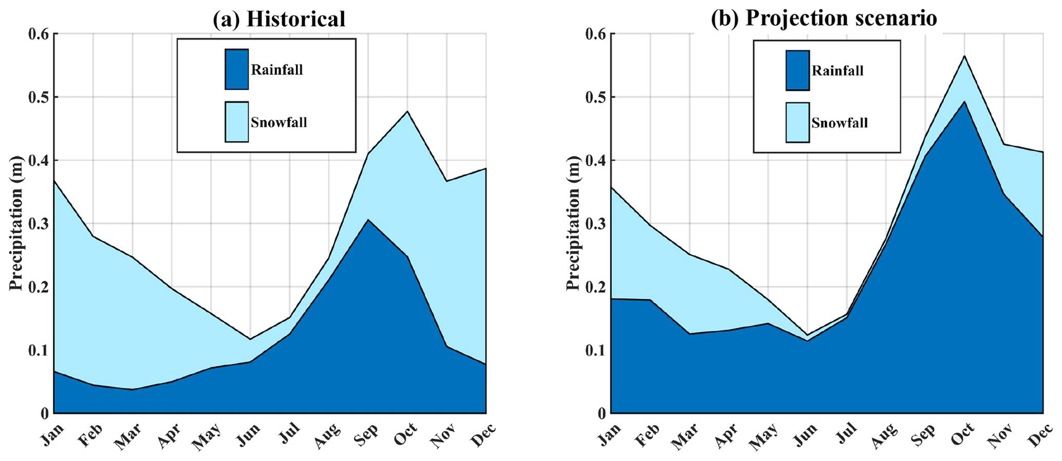
Figure 4Precipitation climatologies. (a) The domain-aggregated GBNPP historical (1979–2015) precipitation climatology, partitioned into snowfall and rainfall constituents. (b) The domain-averaged and domain-aggregated GBNPP projection scenario (2070–2099) precipitation climatology, partitioned into snowfall and rainfall constituents. For all figures, uncertainties are not shown to facilitate readability.
4.3 Changes in glacier coverage
The glacier change map (Fig. 5) displays the static glacier cover used for the historical simulations as well as the static glacier cover used for the projection scenario runs. Recall that SnowModel does not dynamically adjust glacier extent, so these glacier changes represent two distinct landscapes that remain in equilibrium with their environment for the duration of the modeled time period. In the aggregated GBNPP watersheds, the projection scenario contains a 58.8 % decrease in glacier cover compared with the RGI 2014 glacier map, from a total historical surface area of 4092 to 1687 km2 in the projection scenario.

Figure 5Glacier change map. Changes in glacier extent in the study area based on the Randolph Glacier Inventory (RGI) 2014 glacier locations for the historical period (1979–2015) and the +400 m change in equilibrium line altitude for the projection scenario (2070–2099) using RCP 8.5.
4.4 Changes in snow water equivalent
SWE is modeled for the historical and projection scenarios and aggregated for all GBNPP watersheds by mean monthly depth (Fig. 6). Peak SWE historically occurs in April, and while the timing remains unchanged in the projection scenario, GBNPP watersheds lose 46 % of mean peak SWE in the projection scenario. The monthly relative changes in SWE from the historical period to projection scenario range from −44 % in March to −70 % in September. These losses are in line with Shi and Wang's (2015) investigation into Northern Hemisphere changes in SWE based on RCP 8.5 (their Figs. 4c and 6f). The magnitude of the SWE losses in the projection scenario will directly affect the timing and volume of runoff generated from snowmelt.
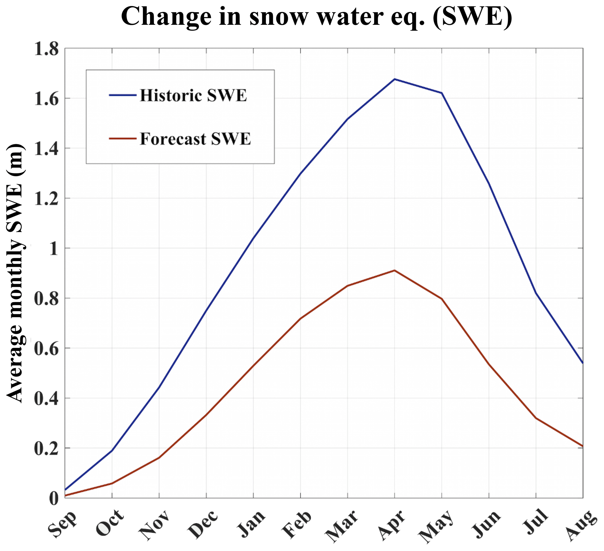
Figure 6Monthly snow water equivalence (m) averaged for the entire GBNPP domain for both the historical (1979–2015) and projection scenario (RCP 8.5; 2070–2099).
4.5 Changes in runoff
The historical runoff hydrograph for GBNPP is partitioned into the components of ice melt, snowmelt, and rain runoff and includes the MODIS-based ET values (Fig. 7a). The historical and projection scenario volumes can be found in Tables 3 and 4, accompanied by the estimated ET values by watershed. The monthly ET values derived from MODIS are included because SnowModel calculates sublimation of the snowpack when solving the energy balance equations but does not calculate ET from the land surface when no snowpack is present. This is why Beamer et al. (2017) added the SoilBal sub-model to their analysis of the Gulf of Alaska SnowModel simulations. Many other previous studies using SnowModel from the Arctic, Patagonia, Greenland, and Alaska do not calculate ET using an additional sub-model, and this paper is no different (Mernild et al., 2012, 2013, 2014, 2017a). These monthly ET values are not subtracted from the partitioned climatologies (snowmelt, glacier melt, rain runoff) because the model does not resolve which of these sources would be the appropriate origin of the ET-based water.
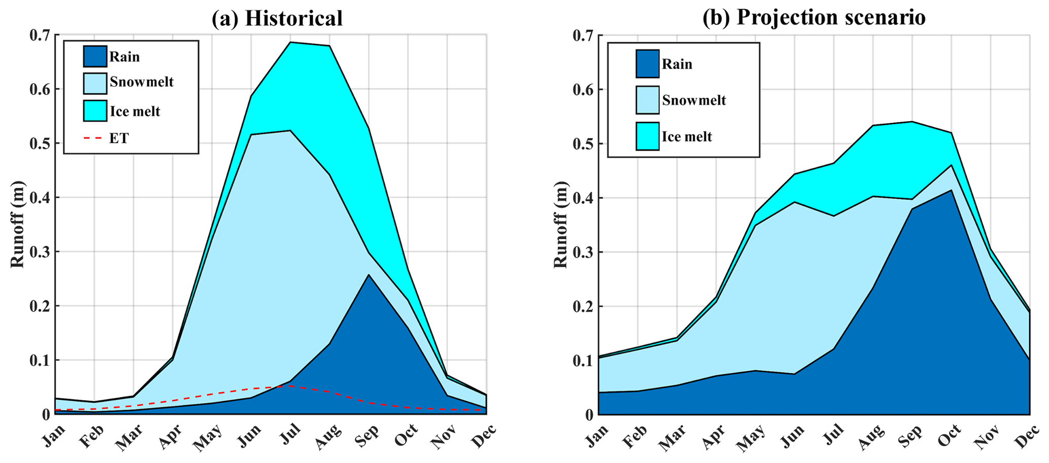
Figure 7Runoff climatologies. (a) The domain-averaged and domain-aggregated historical (1979–2015) GBNPP runoff climatology partitioned into the constituents of snowmelt, ice melt, and rain runoff. The historical (2001–2014) MODIS-based evapotranspiration estimates are included on the historical plots, but the amounts are not subtracted from the modeled runoff climatology because they were derived separately from the modeling process. (b) The domain-averaged and domain-aggregated GBNPP projection scenario (RCP 8.5 scenario; 2070–2099) runoff climatology. Appendix B contains the historical and projection scenario runoff climatologies for each of the eight grouped and individual watersheds in the study area. For all figures, uncertainties are not shown to facilitate readability.
Table 3Historical (1979–2015) and projection scenario (RCP 8.5; 2070–2099) runoff in cubic kilometers (km3) and meters per year (m yr−1) for all watersheds.
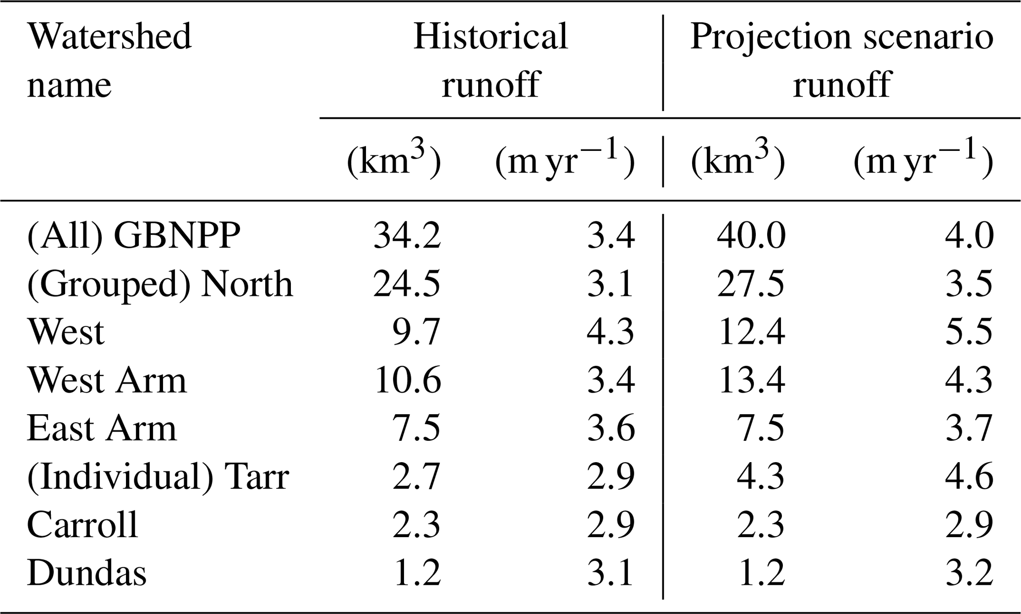
Table 4Estimated historical (2002–2014) and evapotranspiration (ET) in m yr−1 for all watersheds.

The historical runoff hydrograph for GBNPP displays low runoff quantities during the winter months, with snowmelt dominating spring and early summer, ice melt supplementing runoff in midsummer, and rain runoff dominating early fall (Fig. 7a). The average MODIS-based ET loss for GBNPP is 0.28 m yr−1, while the average historical precipitation is 3.40 m yr−1, which makes ET loss 9 % of precipitation on average for all watersheds. The projection scenario runoff total for GBNPP is 3.96 m yr1 and displays a distinct flattening of the annual runoff hydrograph in terms of quantity and timing of snowmelt, as well as a decrease in ice melt to Glacier Bay (Fig. 7b). The historical and projection scenario runoff hydrographs for each grouped and individual watershed can be found in Appendix B, and Fig. 8 presents changes in the runoff components in the projection scenario. In many of the watersheds in the GBNPP domain, there is an overall annual increase of runoff volumes in the projection simulations, with much of that increase sourced from changes in rain runoff. These increases in rain runoff originate from higher temperatures in the projection scenario, losses in glacier area, increases in overall precipitation, and increases in the rainfall component of precipitation.
4.6 Historical freshwater in Glacier Bay
A climatology of the month-to-month changes in FWV (ΔFWV) for various subregions of Glacier Bay is shown in Fig. 9. The seasonal timing of changes in freshwater is similar for all three regions. In assessing the certainty in this ΔFWV signal, it is important to consider that (1) winter is vastly under-sampled as compared to other seasons, and (2) there can be great variability between monthly FWC from year to year. Positive values of ΔFWV are observed in summer months when the strong runoff fluxes from snowmelt and ice melt outpace the ability of water to flush out through the bay mouth. Negative values are observed in winter months when runoff is low, and the bay is able to flush out the accumulated freshwater. The larger values in the West Arm (vs. the East Arm) are due to the larger watershed area, higher mean elevation, and greater glacier coverage. Bear in mind the oceanographic dataset is used qualitatively because of the complex, understudied open boundary of the bay system, where water (fresh and salt) moves freely in and out of the boundary into Icy Strait, the Cross Sound, and eventually the Pacific Ocean. Critically, freshwater fluxes are not measured at the mouth of Glacier Bay, and to the best of the authors' current knowledge, a dataset that includes these fluxes entering and exiting the system does not exist.
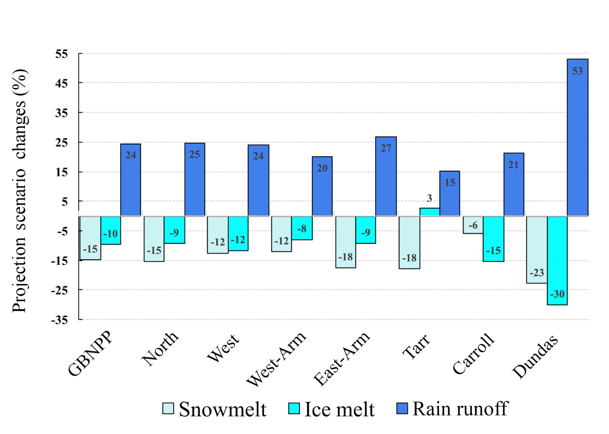
Figure 8Runoff process change by watershed in the projection scenario (RCP 8.5; 2070–2099), partitioned into snowmelt, ice melt, and rain runoff.
Long-term changes in July FWC are also examined. July is chosen since it has the most measurements throughout the bay. Spatially averaged FWC () for various bay subregions is found by interpolating FWC observations across GBNPP and then averaging across each bay subregion for the month of July. Analysis of long-term changes in in all watersheds indicates little change in over the historical study period (1993–2017). The West Arm July observations are the exception, increasing with a rate of 8.3 cm yr−1 (p value of 0.109), but this change is not statistically significant.
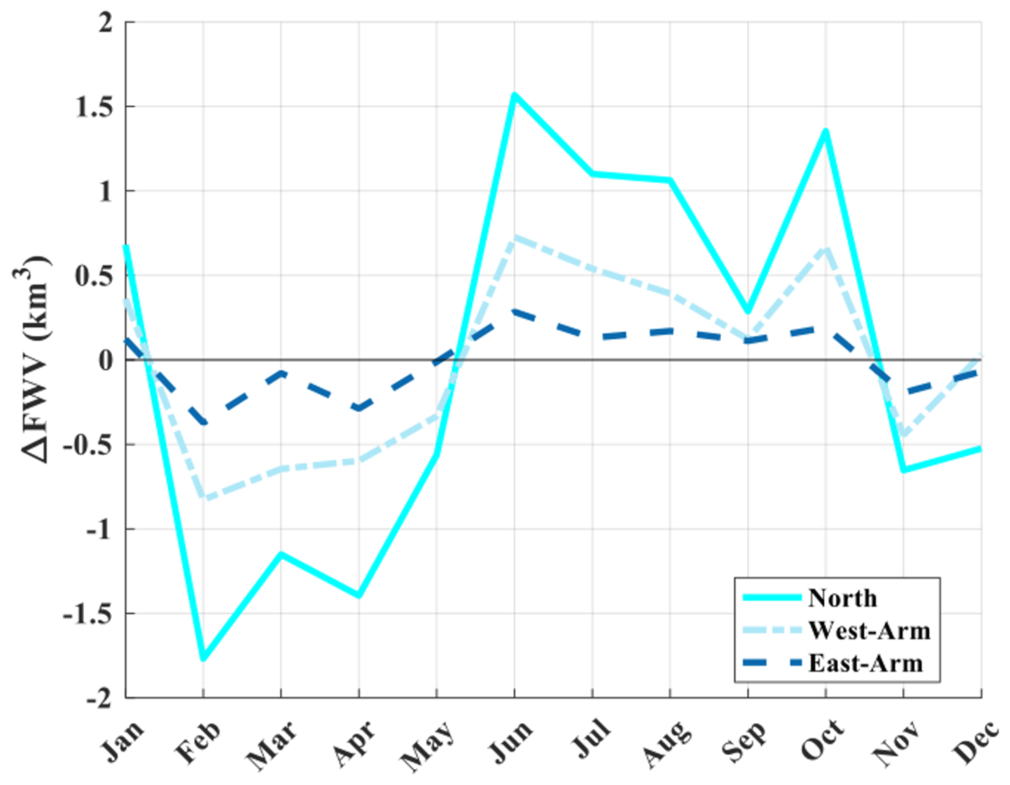
Figure 9Month-to-month changes in freshwater volume (ΔFWV) for the historical period of record (1993 to present) for various subregions (see Fig. 2) of Glacier Bay.
The distinct changes observed in the study area watersheds motivate investigation into the controlling physical characteristics of the various landscapes within GBNPP. For example, in Fig. 3c, the patterns of ΔSFE∕P in the Tarr and Dundas watersheds have opposing seasonal trends. The Tarr watershed has a comparatively high mean elevation and sees only small magnitudes of winter ΔSFE∕P. This may be because much of the watershed remains above the snow line in the projection scenario (see Fig. 10a). Tarr also displays high magnitudes of summer ΔSFE∕P, and it has historically been one of the few watersheds that receives significant snowfall precipitation throughout the summer, again due to the high elevation. As a point of contrast, the Dundas watershed has the lowest mean elevation of the eight study watersheds (see Table 1 and Fig. 10a). Dundas experiences high magnitudes of ΔSFE∕P in the winter but very small magnitudes in the summer. The former is attributable to the projection scenario FLA in Dundas increasing above the maximum watershed elevation, and the latter is due to very small amounts of historical summer snowfall precipitation in Dundas. This initial comparison between the changes in Tarr and Dundas suggests a need to further investigate landscape dependencies and the seasonal aspect of snow precipitation, especially with elevation.

Figure 10Landscape characteristics. (a) Elevation histograms for GBNPP, Tarr, and Dundas watersheds, with the average winter and summer freezing line altitudes (FLA) plotted in blue and red, respectively. Historical scenario (1979–2015) lines are solid, and projection scenario (RCP 8.5; 2070–2099) are dashed. (b) Polar coordinate plots for GBNPP, Tarr, and Dundas displaying the binned aspect and slope distributions within each watershed.
Snow distribution and elevation in mountain environments are highly correlated (Dingman, 1981; Fassnacht et al., 2003; Welch et al., 2013), and in maritime regions, understanding the role of elevation distributions within a watershed is important in the context of changing climate and the snow–rain transition zone (Jefferson, 2011). Histograms of elevation, along with polar coordinate plots of slope and aspect for GBNPP, Dundas, and Tarr are given in Fig. 10 to help illuminate the relationships between elevation, temperature and precipitation change, and process change. Recall that these changes take the form of negative ΔSFE∕P values in all watersheds (Fig. 3c). When considered in relation to the monthly or seasonal average FLA, the magnitudes of the Dundas and Tarr seasonal SFE∕P changes (Fig. 3c) begin to make sense. For this analysis, the most important aspect may be the proportion of the watershed area located between the historical seasonal FLA and projection scenario seasonal FLA. In Dundas, the winter FLA increase of several hundred meters in the projection scenario means that a large proportion of the watershed will receive rainfall when it previously received snowfall. In contrast, when the Tarr watershed is subjected to the same several hundred meter winter FLA increase, only a small proportion of the watershed is affected by that increase (see Fig. 10a), thus undergoing lower magnitudes of ΔSFE∕P than Dundas. The summer FLA increase of >1000 m means that Dundas will likely receive insignificant summer snowfall in the projection scenario, but Tarr will experience higher magnitudes of ΔSFE∕P. This is because a large proportion of the Tarr watershed lies between the historical and projection scenario summer FLAs, but Dundas always received insignificant snowfall historically during the summer. Lastly, the spring (+910 m) and fall (+775 m) ΔFLA represent an increase in the spatial distribution of the rainfall-dominated areas in the projection scenario and are congruent with the changes in temperatures found in Fig. 3a.
Similarly, the distribution of snowpack on the land surface has landscape dependencies on aspect and slope. Regarding topographic slope, Tarr has proportionally more steep slopes than GBNPP and Dundas, and steep slopes tend to accumulate snow in the same locations year after year by way of sloughing, avalanching, and wind drift, distributing snow to the lesser inclined accumulation areas (Fig. 10b; Bloschl and Kirnbauer, 1992; Grünewald el al., 2010, 2014). The average aspect in Tarr is dominated by the northeastern direction, which increases shading and creates more oblique angles of incoming solar radiation, which affects SWE distribution and timing of meltwater. Alternately, the average aspect in GBNPP and Dundas is south to southwestern, and these aspects receive more direct incoming solar radiation angles and will affect accumulation patterns and meltwater patterns differently in these watersheds (Elder et al., 1989; Marks et al., 1999). This study acknowledges these landscape dependencies, and we attempt to briefly characterize some of them as controls on the modeled processes. However, further characterization of the landscape spatial gradients and controls is beyond the scope of this study, while higher-resolution observations and modeling will be necessary to better understand their effects on runoff processes in the future.
This examination of the source components of runoff to Glacier Bay is partially limited by a lack of long-term validation datasets for streamflow and other long-term weather station forcing datasets within the GBNPP model domain. However, an effort to parameterize and calibrate SnowModel based on the results of other recent, larger-scale modeling projects was made, as previously noted in Sect. 3.4 according to Beamer et al. (2016, 2017). While implementation of SnowModel using additional validation and forcing datasets would likely improve the accuracy of the results, no regional streamflow, SWE observations, or weather station datasets exist at the appropriate locations or timescales. This highlights the need for multiple types of monitoring systems to be implemented in GBNPP in order to decipher future changes in glaciers, snowpack and precipitation, and runoff processes in GBNPP. Additionally, other important fluxes are not characterized in this study due to decisions in the modeling process, most notably snow density characterization which allows for rain-on-snow (ROS) events to be examined. For the present study, when rain precipitation occurs on top of an existing snowpack, ROS is characterized simply as increasing the SWE in the snowpack. Even though it is known that ROS runoff events generally occur at snow densities greater than ∼550 kg m−3, the final results do not describe the volume or frequency of ROS events since the snow density output is not necessary or desirable for our research interests. However, the results of this study reveal a shift from snowmelt-dominated runoff historically to rain runoff in the projection scenarios, and understanding the timing and spatial extent of ROS events may prove to be an important area of research in the future.
We include the historical freshwater analysis of Glacier Bay because long-term meteorological datasets or streamflow datasets do not exist for the study area. The inclusion of the observational CTD dataset allows the modeling effort to be contextualized. The most notable is the monthly timing of the historical runoff in GBNPP (Fig. 7a) as it relates to the monthly fluctuations of freshwater volumes from the CTD analysis (Fig. 9). Not only is the runoff timing confirmed by the observations, but the relative magnitude of the proportion of freshwater originating from the West Arm and East Arm watersheds is also confirmed by the observations (Figs. 7a, 9). Since the modeled runoff volumes for the projection scenario (Fig. 7b; Appendix B) exhibit differences in timing and magnitude from the historical model runs (Fig. 7a; Appendix B), we can assume that the influx of freshwater from the land surface to Glacier Bay in the projection scenario will reflect those changes in timing and magnitude. From the historical simulations, July is the month with the most combined runoff from the various freshwater sources. The modeled changes in timing and magnitude of runoff from the land surface into Glacier Bay will have effects on bay ecology in the future if the projection scenario climate conditions come to pass.
A key source of uncertainty in the present study is the determination of the future glacier cover. We rely on the findings of Beamer et al. (2017) to guide assumptions of future ELA increases and AAR changes, if any. Their decisions are, in turn, based on regional-scale (Alaska-wide) modeling studies of glacier change (Huss and Hock, 2015) and on decadal-scale observational studies of glacier mass balance based on altimetry (Larsen et al., 2015) and gravimetry (Arendt et al., 2008). Our results for GBNPP show a change of −58 % in glacier-covered area. Huss and Hock (2015) give a figure of −32 % for change in glacier volume in all of Alaska. Comparisons between these two values are difficult, given that they are for different domains (local vs. regional) and for different variables (area vs. volume). Furthermore, the SnowModel simulations rely on a single glacier cover extent for the 36-year historical period and the 30-year projection scenario, while in reality glaciers respond to climatic forcings in a dynamic and continuous way on daily, seasonal, and annual timescales. This is a simplification due to the fact that (1) high-resolution input data at the appropriate spatial and temporal scales are computationally expensive and nonexistent; (2) changing the land cover (i.e., glacier extent) would require additional, year-by-year glacier dynamics modeling in the study area; and (3) previous decadal-scale studies using SnowModel also assume static land cover over the time period of interest (Beamer et al., 2017; Mernild et al., 2017a–d). To the best of our knowledge, local-scale modeling studies of glacier change in GBNPP are not available and outside the scope of the present study. We note the work of Alifu et al. (2016), who use a variety of remote sensing products to quantify observational changes in mean snow line altitude (MSLA) and mean snow accumulation area ratio in GBNPP during 2000–2012. Their results support the general trends of the present study, in terms of reductions in area change and increases in MSLA, but the duration of their study is quite short in comparison to the century-scale processes investigated in the present study.
In this study, a high spatial resolution, distributed snow evolution and ablation model, SnowModel, is used to estimate current and future freshwater runoff into Glacier Bay, Alaska. The model is forced using the MERRA weather reanalysis product to create 36-year historical climatologies of precipitation, temperature, and the source components of runoff, including rainfall, snowmelt, and ice melt. The future scenario applies the SNAP temperature and precipitation anomalies from the mean of five climate models for the years 2070–2099 based on RCP 8.5. The physical complexity and variability of the region produce a variety of historical and projection scenario hydrographs within GBNPP, including rainfall-, snowmelt-, and ice-melt-dominated responses depending on the season and watershed. The timing and relative scaling of the historical inputs of freshwater from the study area watersheds are contextualized by a long-term oceanographic dataset from the Southeast Alaska Inventory and Monitoring Network in Glacier Bay. The mean annual runoff to Glacier Bay in the projection scenario will increase by 13 % from the historical average, with much of the increased runoff sourced from rain inputs. The peak flows to the Glacier Bay fjord estuary will shift from late summer to early fall, and the effects of these changes in freshwater runoff timing will be experienced across the estuarine environment and biological communities within Glacier Bay.
Numerous online datasets were used for this project and can be found at the following locations.
-
Shuttle Radar Topography Mission (SRTM) digital elevation model: http://srtm.csi.cgiar.org/srtmdata/ (Farr et al., 2007).
-
North American Land Change Monitoring System (NALCMS) landcover dataset: https://catalog.data.gov/dataset/north-american-land-change-monitoring-system-nalcms-collection (Latifovic et al., 2010).
-
MERRA Reanalysis dataset: https://disc.gsfc.nasa.gov/datasets?page=1&keywords=merra (Rienecker et al., 2011).
-
CFSR Reanalysis dataset: https://rda.ucar.edu/datasets/ds093.1/#!description (Saha et al., 2010b).
-
Evapotranspiration MODIS (MOD16A2) dataset: https://lpdaac.usgs.gov/products/mod16a2v006/ (Running et al., 2017). This dataset was accessed using Google Earth Engine at https://developers.google.com/earth-engine/datasets/catalog/MODIS_006_MOD16A2, last access: 10 June 2019.
-
Oceanographic Southeast Alaska Inventory & Monitoring Network (SEAN) dataset: https://www.nps.gov/im/sean/oceanography.htm (Johnson and Stachura, 2011).
-
Randolf Glacier Inventory (RGI 4.0) dataset: https://www.glims.org/RGI/ (RGI Consortium, 2017).
-
Scenarios Network for Alaska and Arctic Planning (SNAP) dataset: https://www.snap.uaf.edu/tools-data/data-downloads (Scenarios Network for Alaska and Arctic Planning, 2019).
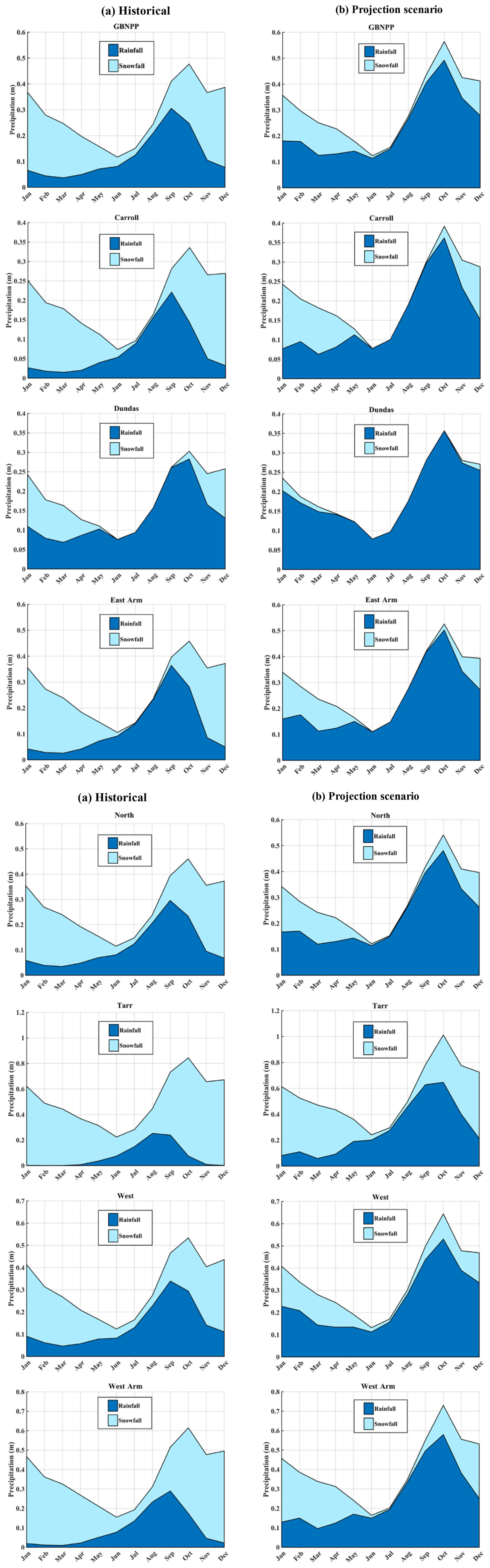
Figure A1(a) The historical precipitation climatologies by watershed, partitioned into snowfall and rainfall constituents. (b) The projection scenario precipitation climatologies by watershed, partitioned into snowfall and rainfall constituents.

Figure B1(a) The historical runoff climatologies by watershed, partitioned into the constituents of snowmelt, ice melt, and rain runoff. The historical MODIS-based evapotranspiration estimates are included on the historical plots, but the amounts are not subtracted from the modeled for runoff climatology because they were derived separately from the modeling process. (b) The projection scenario runoff climatologies by watershed.
RLC and DFH designed the research questions, chose the methods, and oversaw the analysis of the results for the paper. JPB and RLC developed the scripts that were applied to the model output and performed the model simulations. ERH contributed the oceanographic data analysis. RLC prepared the paper with contributions from all co-authors.
The authors declare that they have no conflict of interest.
Funding for this study was provided by the National Park Service and Glacier Bay National Park and Preserve under Pacific Northwest CESU agreement no. HBW07110001 and federal grant no. P15AC01065.
This research has been supported by the National Park Service (Pacific Northwest CESU agreement no. HBW07110001 and federal grant no. P15AC01065).
This paper was edited by Daniel Farinotti and reviewed by Janet Curran, Kristian Förster, and one anonymous referee.
Alifu, H., Tateishi, R., Nduati, E., and Maitiniyazi, A.: Glacier changes in Glacier Bay, Alaska, during 2000–2012, Int. J. Remote Sens., 37, 4132–4147, https://doi.org/10.1080/01431161.2016.1207267, 2016.
Arendt, A., Walsh, J., and Harrison, W.: Changes of glaciers and climate in northwestern North America during the late twentieth century, J. Climate, 22, 4117–4134, https://doi.org/10.1175/2009JCLI2784.1, 2009.
Arendt, A. A., Echelmeyer, K. A., Harrison, W. D., Lingle, C. S., and Valentine, V. B.: Rapid wastage of Alaska glaciers and their contribution to rising sea level, Science, 297, 382–386, https://doi.org/10.1126/science.1072497, 2002.
Arendt, A. A., Luthcke, S. B., Larsen, C. F., Abdalati, W., Krabill, W. B., and Beedle, M. J.: Validation of high-resolution GRACE mascon estimates of glacier mass changes in the St Elias Mountains, Alaska, USA, using aircraft laser altimetry, J. Glaciol., 54, 778–787, https://doi.org/10.3189/002214308787780067, 2008.
Barnes, S. L.: A technique for maximizing details in numerical weather map analysis, J. Appl. Meteorol., 3, 396–409, https://doi.org/10.1175/1520-0450(1964)003<0396:ATFMDI>2.0.CO;2, 1964.
Barnes, S. L.: Mesoscale objective map analysis using weighted time-series observations, Technical Report, National Severe Storms Lab., Norman, Oklahoma, 1973.
Beamer, J. P., Hill, D. F., Arendt, A., and Liston, G. E.: High-resolution modeling of coastal freshwater discharge and glacier mass balance in the Gulf of Alaska watershed, Water Resour. Res., 52, 3888–3909, https://doi.org/10.1002/2015WR018457, 2016.
Beamer, J. P., Hill, D. F., McGrath, D., Arendt, A., and Kienholz, C.: Hydrologic impacts of changes in climate and glacier extent in the Gulf of Alaska watershed, Water Resour. Res., 53, 7502–7520, https://doi.org/10.1002/2016WR020033, 2017.
Bloschl, G. and Kirnbauer, R.: An analysis of snow cover patterns in a small alpine catchment, Hydrol. Process., 6, 99–109, https://doi.org/10.1002/hyp.3360060109, 1992.
Carmack, E., McLaughlin, F., Yamamoto-Kawai, M., Itoh, M., Shimada, K., Krishfield, R., and Proshutinsky, A.: Freshwater storage in the Northern Ocean and the special role of the Beaufort Gyre, in: Arctic–subArctic ocean fluxes Springer, Dordrecht, 145–169, https://doi.org/10.1007/978-1-4020-6774-7_8, 2008.
Carmack, E. C.: The alpha/beta ocean distinction: A perspective on freshwater fluxes, convection, nutrients and productivity in high-latitude seas, Deep-Sea Res Pt. II, 54, 2578–2598, https://doi.org/10.1016/j.dsr2.2007.08.018, 2007.
Chapin, F. S., Walker, L. R., Fastie, C. L., and Sharman, L. C.: Mechanisms of primary succession following deglaciation at Glacier Bay, Alaska, Ecol. Monogr., 64, 149–175, https://doi.org/10.2307/2937039, 1994.
Clarke, G. K. C., Jarosch, A. H., Anslow, F. S., Radić, V., and Menounos, B.: Projected deglaciation of western Canada in the twenty-first century, Nat. Geosci., 8, 372–377, https://doi.org/10.1038/ngeo2407, 2015.
Curran, J. H., Meyer, D. F., and Tasker, G. D.: Estimating the magnitude and frequency of peak streamflows for ungaged sites on streams in Alaska and conterminous basins in Canada, Water-Resources Investigations Report, 3, p. 4188, 2003.
Dai, A., Qian, T., Trenberth, K. E., and Milliman, J. D.: Changes in continental freshwater discharge from 1948 to 2004, J. Climate, 22, 2773–2792, https://doi.org/10.1175/2008JCLI2592.1, 2009.
Dee, D. P., Uppala, S. M., Simmons, A. J., Berrisford, P., Poli, P., Kobayashi, S., Andrae, U., Balmaseda, M. A., Balsamo, G., Bauer, P., and Bechtold, P.: The ERA-Interim reanalysis: Configuration and performance of the data assimilation system, Q. J. Roy. Meteor. Soc., 137, 553–597, https://doi.org/10.1002/qj.828, 2011.
Dingman, S. L.: Elevation: a major influence on the hydrology of New Hampshire and Vermont, USA, Hydrolog. Sci. J., 26, 399–413, https://doi.org/10.1080/02626668109490904, 1981.
Elder, K., Dozier, J., and Michaelsen, J.: Spatial and temporal variation of net snow accumulation in a small alpine watershed, Emerald Lake basin, Sierra Nevada, California, USA, Ann. Glaciol., 13, 56–63, https://doi.org/10.3189/S0260305500007643, 1989.
Etherington, L. L., Hooge, P. N., Hooge, E. R., and Hill, D. F.: Oceanography of Glacier Bay, Alaska: implications for biological patterns in a glacial fjord estuary, Estuar. Coasts, 30, 927–944, https://doi.org/10.1007/BF02841386, 2007.
Farr, T. G., Rosen, P. A., Caro, E., Crippen, R., Duren, R., Hensley, S., Kobrick, M., Paller, M., Rodriguez, E., Roth, L., and Seal, D.: The shuttle radar topography mission, Rev. Geophys., 45, RG2004, https://doi.org/10.1029/2005RG000183, 2007.
Fassnacht, S. R., Dressler, K. A., and Bales, R. C.: Snow water equivalent interpolation for the Colorado River Basin from snow telemetry (SNOTEL) data, Water Resour. Res., 39, 1208, https://doi.org/10.1029/2002WR001512, 2003.
Fissel, B., Dalton, M., Felthoven, R., Garber-Yonts, B., Haynie, A., Himes-Cornell, A., and Seung, C.: Stock assessment and fishery evaluation report for the groundfish fisheries of the Gulf of Alaska and Bering Sea/Aleutian Islands Area: economic status of the groundfish fisheries off Alaska, 2013, National Marine Fisheries Service, Economic and Social Sciences Research Program, Seattle, 2014.
Fowler, H., Bleinkinsop, S., and Tebaldi, C.: “Review – linking climate change modeling to impacts studies: recent advances in downscaling techniques for hydrological modeling”, Int. J. Climatol., 27, 1547–1578, https://doi.org/10.1002/joc.1556, 2007.
Gardner, A. S., Moholdt, G., Cogley, J. G., Wouters, B., Arendt, A. A., Wahr, J., Berthier, E., Hock, R., Pfeffer, W. T., Kaser, G., and Ligtenberg, S. R.: A reconciled estimate of glacier contributions to sea level rise: 2003 to 2009, Science, 340, 852–857, https://doi.org/10.1126/science.1234532, 2013.
Grünewald, T., Schirmer, M., Mott, R., and Lehning, M.: Spatial and temporal variability of snow depth and ablation rates in a small mountain catchment, The Cryosphere, 4, 215–225, https://doi.org/10.5194/tc-4-215-2010, 2010.
Grünewald, T., Bühler, Y., and Lehning, M.: Elevation dependency of mountain snow depth, The Cryosphere, 8, 2381–2394, https://doi.org/10.5194/tc-8-2381-2014, 2014.
Hall, D. K., Benson, C. S., and Field, W. O.: Changes of glaciers in Glacier Bay, Alaska, using ground and satellite measurements, Phys. Geogr., 16, 27–41, https://doi.org/10.1080/02723646.1995.10642541, 1995.
Hill, D. F., Ciavola, S. J., Etherington, L., and Klaar, M. J.: Estimation of freshwater runoff into Glacier Bay, Alaska and incorporation into a tidal circulation model, Estuar. Coastal Shelf S., 82, 95–107, https://doi.org/10.1016/j.ecss.2008.12.019, 2009.
Huss, M. and Hock, R.: A new model for global glacier change and sea-level rise, Cryospheric Sci., 3, 54, https://doi.org/10.3389/feart.2015.00054, 2015.
Jefferson, A. J.: Seasonal versus transient snow and the elevation dependence of climate sensitivity in maritime mountainous regions, Geophys. Res. Lett., 38, L16402, https://doi.org/10.1029/2011GL048346, 2011.
Johnson, W. and Sharman, L.: Glacier Bay National Park and Preserve oceanographic monitoring protocol: Version OC-2014.1, Natural Resource Report, NPS/SEAN/NRR–2014/851, National Park Service, Fort Collins, Colorado, 2014.
Johnson, W. F. and Stachura, M. M.: Creation of Glacier Bay oceanographic information products defined in protocol OC-2010.1 using legacy data covering 1993 through 2008: methods, quality levels, and exceptions, Natural Resource Data Series, NPS/SEAN/NRDS—2011/130, National Park Service, Natural Resource Program Center, Fort Collins, Colorado, available at: https://www.nps.gov/im/sean/oceanography.htm (last access: 10 June 2019), 2011.
Kalnay, E., Kanamitsu, M., Kistler, R., Collins, W., Deaven, D., Gandin, L., Iredell, M., Saha, S., White, G., Woollen, J., and Zhu, Y.: The NCEP/NCAR 40-year reanalysis project, B. Am. Meteorol. Soc., 77, 437–471, https://doi.org/10.1175/1520-0477(1996)077<0437:TNYRP>2.0.CO;2, 1996.
Knowles, N., Dettinger, M. D., and Cayan, D. R.: Trends in snowfall versus rainfall in the western United States, J. Climate, 19, 4545–4559, https://doi.org/10.1175/JCLI3850.1, 2006.
Latifovic, R., Homer, C., Ressl, R., Pouliot, D., Hossain, S.N., Colditz Colditz, R. R., Olthof, I., Giri, C., and Victoria, A.: North American land change monitoring system (NALCMS), Remote sensing of land use and land cover: principles and applications, CRC Press, Boca Raton, available at: https://catalog.data.gov/dataset/north-american-land-change-monitoring-system-nalcms-collection (last access: 10 June 2019), 2010.
Lader, R., Bhatt, U. S., Walsh, J. E., Rupp, T. S., and Bieniek, P. A.: Two-meter temperature and precipitation from atmospheric reanalysis evaluated for Alaska, J. Appl. Meteorol. Climatol., 55, 901–922, https://doi.org/10.1175/JAMC-D-15-0162.1, 2016.
Larsen, C. F., Motyka, R. J., Freymueller, J. T., Echelmeyer, K. A., and Ivins, E. R.: Rapid viscoelastic uplift in southeast Alaska caused by post-Little Ice Age glacial retreat, Earth Planet. Sc. Lett., 237, 548–560, https://doi.org/10.1016/j.epsl.2005.06.032, 2005.
Larsen, C. F., Burgess, E., Arendt, A. A., O'Neel, S., Johnson, A. J., and Kienholz, C.: Surface melt dominates Alaska glacier mass balance, Geophys. Res. Lett., 42, 5902–5908, https://doi.org/10.1002/2015GL064349, 2015.
Lim, E., Eakins, B. W., and Wigley, R.: Coastal Relief Model of Southern Alaska: Procedures, Data Sources and Analysis, NOAA Technical Memorandum NESDIS NGDC-43, 22 pp., August 2011.
Liston, G. E. and Elder, K.: A meteorological distribution system for high-resolution terrestrial modeling (MicroMet), J. Hydrometeorol.,7, 217–234, https://doi.org/10.1175/JHM486.1, 2006a.
Liston, G. E. and Elder, K.: A distributed snow-evolution modeling system (SnowModel), J. Hydrometeorol., 7, 1259–1276, https://doi.org/10.1175/JHM548.1, 2006b.
Liston, G. E. and Hiemstra, C. A.: The changing cryosphere: Pan-Arctic snow trends (1979–2009), J. Climate, 24, 5691–5712, https://doi.org/10.1175/JCLI-D-11-00081.1, 2011.
Liston, G. E. and Mernild, S. H.: Greenland freshwater runoff. Part I: A runoff routing model for glaciated and nonglaciated landscapes (HydroFlow), J. Climate, 25, 5997–6014, https://doi.org/10.1175/JCLI-D-11-00591.1, 2012.
Luthcke, S. B., Sabaka, T. J., Loomis, B. D., Arendt, A. A., McCarthy, J. J., and Camp, J.: Antarctica Greenland and Gulf of Alaska land-ice evolution from an iterated GRACE global mascon solution, J. Glaciol., 59, 613–631, https://doi.org/10.3189/2013JoG12J147, 2013.
Marks, D., Domingo, J., Susong, D., Link, T., and Garen, D.: A spatially distributed energy balance snowmelt model for application in mountain basins, Hydrol. Process., 13, 1935–1959, https://doi.org/10.1002/(SICI)1099-1085(199909)13:12/13<1935::AID-HYP868>3.0.CO;2-C, 1999.
McGrath, D., Sass, L., O'Neel, S., Arendt, A., and Kienholz, C.: Hypsometric control on glacier mass balance sensitivity in Alaska and northwest Canada, Earth's Future, 5, 324–336, https://doi.org/10.1002/2016EF000479, 2017.
McPhee, M. G., Proshutinsky, A., Morison, J. H., Steele, M., and Alkire, M. B.: Rapid change in freshwater content of the Arctic Ocean, Geophys. Res. Lett., 36, L10602, https://doi.org/10.1029/2009GL037525, 2009.
Mernild, S. H. and Liston, G. E.: Greenland freshwater runoff. Part II: Distribution and trends, 1960–2010, J. Climate, 25, 6015–6035, https://doi.org/10.1175/JCLI-D-11-00592.1, 2012.
Mernild, S. H., Liston, G. E., Hiemstra, C. A., Christensen, J. H., Stendel, M., and Hasholt, B.: Surface mass balance and runoff modeling using HIRHAM4 RCM at Kangerlussuaq (Søndre Strømfjord), West Greenland, 1950–2080, J. Climate, 24, 609–623, https://doi.org/10.1175/2010JCLI3560.1, 2011.
Mernild, S. H., Lipscomb, W. H., Bahr, D. B., Radić, V., and Zemp, M.: Global glacier changes: a revised assessment of committed mass losses and sampling uncertainties, The Cryosphere, 7, 1565–1577, https://doi.org/10.5194/tc-7-1565-2013, 2013.
Mernild, S. H., Liston, G. E., and Hiemstra, C. A.: Northern hemisphere glacier and ice cap surface mass balance and contribution to sea level rise, J. Climate, 27, 6051–6073, https://doi.org/10.1175/JCLI-D-13-00669.1, 2014.
Mernild, S. H., Liston, G. E., Hiemstra, C. A., Malmros, J. K., Yde, J. C., and McPhee, J.: The Andes Cordillera. Part I: snow distribution, properties, and trends (1979–2014), Int. J. Climatol., 37, 1680–1698, https://doi.org/10.1002/joc.4804, 2017a.
Mernild, S. H., Liston, G. E., Hiemstra, C.A., Yde, J. C., McPhee, J., and Malmros, J. K.: The Andes Cordillera. Part II: Rio Olivares Basin snow conditions (1979–2014), central Chile, Int. J. Climatol., 37, 1699–1715, https://doi.org/10.1002/joc.4828, 2017b.
Mernild, S. H., Liston, G. E., Hiemstra, C., and Wilson, R.: The Andes Cordillera. Part III: glacier surface mass balance and contribution to sea level rise (1979–2014), Int. J. Climatol., 37, 3154–3174, https://doi.org/10.1002/joc.4907, 2017c.
Mernild, S. H., Liston, G. E., Hiemstra, C., Beckerman, A. P., Yde, J. C., and McPhee, J.: The Andes Cordillera. Part IV: spatio-temporal freshwater run-off distribution to adjacent seas (1979–2014), Int. J. Climatol., 37, 3175–3196, https://doi.org/10.1002/joc.4922, 2017d.
Mesinger, F., DiMego, G., Kalnay, E., Mitchell, K., Shafran, P. C., Ebisuzaki, W., Jović, D., Woollen, J., Rogers, E., Berbery, E. H., and Ek, M. B.: North American regional reanalysis, B. Am. Meteorol. Soc., 87, 343–360, https://doi.org/10.1175/BAMS-87-3-343, 2006.
Mote, P. W.: Trends in snow water equivalent in the Pacific Northwest and their climatic causes, Geophys. Res. Lett., 30, 1601, https://doi.org/10.1029/2003GL017258, 2003.
Mote, P. W., Hamlet, A. F., Clark, M. P., and Lettenmaier, D. P.: Declining mountain snowpack in western North America, B. Am. Meteorol. Soc., 86, 39–49, https://doi.org/10.1175/BAMS-86-1-39, 2005.
Motyka, R. J., O'Neel, S., Connor, C. L., and Echelmeyer, K. A.: Twentieth century thinning of Mendenhall Glacier, Alaska, and its relationship to climate, lake calving, and glacier run-off, Global Planet. Change, 35, 93–112, https://doi.org/10.1016/S0921-8181(02)00138-8, 2003.
Mpelasoka, F. S. and Chiew, F. H.: Influence of rainfall scenario construction methods on runoff projections, J. Hydrometeorol., 10, 1168–1183, https://doi.org/10.1175/2009JHM1045.1, 2009.
Neal, E. G., Hood, E., and Smikrud, K.: Contribution of glacier runoff to freshwater discharge into the Gulf of Alaska, Geophys. Res. Lett., 37, L06404, https://doi.org/10.1029/2010GL042385, 2010.
O'Neel, S., Hood, E., Bidlack, A. L., Fleming, S. W., Arimitsu, M. L., Arendt, A., Burgess, E., Sergeant, C. J., Beaudreau, A. H., Timm, K., and Hayward, G. D.: Icefield-to-ocean linkages across the northern Pacific coastal temperate rainforest ecosystem, Bioscience, 65, 499–512, https://doi.org/10.1093/biosci/biv027, 2015.
Paul, F., Maisch, M., Rothenbühler, C., Hoelzle, M., and Haeberli, W.: Calculation and visualisation of future glacier extent in the Swiss Alps by means of hypsographic modelling, Global Planet. Change, 55, 343–357, https://doi.org/10.1016/j.gloplacha.2006.08.003, 2007.
Pfeffer, W. T., Arendt, A. A., Bliss, A., Bolch, T., Cogley, J. G., Gardner, A. S., Hagen, J. O., Hock, R., Kaser, G., Kienholz, C., Miles, E. S., Moholdt, G., Mölg, N., Paul, F., Radić, V., Rastner, P., Raup, B. H., Rich, J., Sharp, M. J., and the Randolph Consortium: The Randolph Glacier Inventory: a globally complete inventory of glaciers, J. Glaciol., 60, 537–551, https://doi.org/10.3189/2014JoG13J176, 2014.
Radić, V. and Hock, R.: Regional and global volumes of glaciers derived from statistical upscaling of glacier inventory data, J. Geophys. Res.-Earth, 115, F01010, https://doi.org/10.1029/2009JF001373, 2010.
Reisdorph, S. C. and Mathis, J. T.: The dynamic controls on carbonate mineral saturation states and ocean acidification in a glacially dominated estuary, Estuar. Coast. Shelf S., 144, 8–18, https://doi.org/10.1016/j.ecss.2014.03.018, 2014.
RGI Consortium: Randolph Glacier Inventory – A Dataset of Global Glacier Outlines: Version 6.0: Technical Report, Global Land Ice Measurements from Space, Colorado, USA, https://doi.org/10.7265/N5-RGI-60m, 2017.
Rienecker, M. M., Suarez, M. J., Gelaro, R., Todling, R., Bacmeister, J., Liu, E., Bosilovich, M. G., Schubert, S. D., Takacs, L., Kim, G. K., and Bloom, S.: MERRA: NASA's modern-era retrospective analysis for research and applications, J. Climate, 24, 3624–3648, https://doi.org/10.1175/JCLI-D-11-00015.1, 2011.
Running, S., Mu, Q., and Zhao, M.: MOD16A2 MODIS/Terra Net Evapotranspiration 8-Day L4 Global 500 m SIN Grid V006 [Data set], NASA EOSDIS Land Processes DAAC, https://doi.org/10.5067/MODIS/MOD16A2.006, 2017.
Saha, S., Moorthi, S., Pan, H. L., Wu, X., Wang, J., Nadiga, S., Tripp, P., Kistler, R., Woollen, J., Behringer, D., and Liu, H.: The NCEP climate forecast system reanalysis, B. Am. Meteorol. Soc., 91, 1015–1057, https://doi.org/10.1175/2010BAMS3001.1, 2010a.
Saha, S., Moorthi, S., Pan, H., Wu, X., Wang, J., Nadiga, S., Tripp, P., Kistler, R., Woollen, J., Behringer, D., Liu, H., Stokes, D., Grumbine, R., Gayno, G., Wang, J., Hou, Y., Chuang, H., Juang, H. H., Sela, J., Iredell, M., Treadon, R., Kleist, D., Delst, P. V., Keyser, D., Derber, J., Ek, M., Meng, J., Wei, H., Yang, R., Lord, S., van den Dool, H., Kumar, A., Wang, W., Long, C., Chelliah, M., Xue, Y., Huang, B., Schemm, J., Ebisuzaki, W., Lin, R., Xie, P., Chen, M., Zhou, S., Higgins, W., Zou, C., Liu, Q., Chen, Y., Han, Y., Cucurull, L., Reynolds, R. W., Rutledge, G., and Goldberg, M.: NCEP Climate Forecast System Reanalysis (CFSR) Selected Hourly Time-Series Products, January 1979 to December 2010, Research Data Archive at the National Center for Atmospheric Research, Computational and Information Systems Laboratory, https://doi.org/10.5065/D6513W89, 2010b.
Shi, H. X. and Wang, C. H.: Projected 21st century changes in snow water equivalent over Northern Hemisphere landmasses from the CMIP5 model ensemble, The Cryosphere, 9, 1943–1953, https://doi.org/10.5194/tc-9-1943-2015, 2015.
Scenarios Network for Alaska and Arctic Planning: University of Alaska, available at: https://www.snap.uaf.edu/tools-data/data-downloads, last access: 6 June 2019.
Weingartner, T. J., Danielson, S. L., and Royer, T. C.: Freshwater variability and predictability in the Alaska Coastal Current, Deep-Sea Res. Pt II, 52, 169–191, https://doi.org/10.1016/j.dsr2.2004.09.030, 2005.
Welch, S. C., Kerkez, B., Bales, R. C., Glaser, S. D., Rittger, K., and Rice, R. R.: Sensor placement strategies for snow water equivalent (SWE) estimation in the American River basin, Water Resour. Res., 49, 891–903, https://doi.org/10.1002/wrcr.20100, 2013.
Wessel, P. and Bercovici, D.: Interpolation with splines in tension: a Green's function approach, Math. Geol., 30, 77–93, https://doi.org/10.1023/A:1021713421882, 1998.
Wiley, J. B. and Curran, J. H.: Estimating annual high-flow statistics and monthly and seasonal low-flow statistics for ungauged sites on streams in Alaska and conterminous basins in Canada, Water-Resources Investigations Report, 3, p. 4114, 2003.
Zhang, X., Vincent, L. A., Hogg, W. D., and Niitsoo, A.: Temperature and precipitation trends in Canada during the 20th century, Atmos. Ocean, 38, 395–429, https://doi.org/10.1080/07055900.2000.9649654, 2000.
Ziemen, F. A., Hock, R., Aschwanden, A., Khroulev, C., Kienholz, C., Melkonian, A., and Zhang, J.: Modeling the evolution of the Juneau Icefield between 1971 and 2100 using the Parallel Ice Sheet Model (PISM), J. Glaciol., 62, 199–214, https://doi.org/10.1017/jog.2016.13, 2016.