2.1 Buoy data

IMBs autonomously measure thermodynamic changes in sea ice mass balance (Richter-Menge et al., 2006; Polashenski et al., 2011). They are part of a network of drifting buoys over the Arctic Ocean that provide meteorological and oceanographic data for real-time operational requirements and research purposes (Rigor et al., 2000). These instruments typically record GPS position, T2M and mean sea level pressure (MSLP) at hourly intervals, as well as temperature profiles through the air, snow, ice, and upper-ocean and distances to snow/ice surface and ice bottom at 4 h intervals. Snow depth and ice thickness can be estimated from the distances measured by acoustic sounders, if the initial thickness of snow and ice is known when the IMB is deployed (Wang et al., 2013). If the acoustic sounders fail but the temperature string works, the positions of the ice surface and bottom can be determined from the temperature readings. Similar to IMBs, snow buoys also record GPS position, T2M, MSLP and snow depth at hourly intervals (Grosfeld et al., 2016; Nicolaus et al., 2017). However, snow buoys do not measure temperature profiles, and provide no information on ice thickness.

Since 2000, a large number of IMBs have been deployed across the Arctic, in regions such as the central Arctic, the Beaufort Sea, the Chukchi Sea, the Laptev Sea, the North Pole, Canadian Islands and Svalbard (Perovich et al., 2017; http://imb-crrel-dartmouth.org/archived-data/, last access: 15 October 2017). In this study, we use data from 13 IMBs deployed in these different regions between 2010 and 2015 (Fig. 1, Table 1). The IMBs were typically deployed in the central Arctic during April–May, while deployments in the Beaufort, Laptev and Chukchi seas generally took place in August–September (Fig. 1, Table 1). For additional coverage, we also use observations from three snow buoys deployed in 2015, two of which were in the Laptev Sea and one in the central Arctic (Table 1; Fig. 1) (http://www.meereisportal.de/en, last access: 17 January 2018). For simplicity, hereafter we refer to IMBs and snow buoys as buoys.

Figure 1Drift trajectories of all selected buoys (IMBs and snow buoys) in 2010 to 2015. The symbol “⋆” indicates the start of the drift and “∘” signals the end of the drift. Buoys are labelled at the beginning or the end of the drift using the same colour as trajectories. Buoys used for model simulations are highlighted with a solid thick line and bold font. Dashed thick lines illustrate our definition for sectors: central Arctic (black; north of 86^∘ N), and south of 86^∘ N: Pacific sector (magenta; 90^∘ W–150^∘ E), Atlantic sector (cyan; 30^∘ W–60^∘ E) and Laptev Sea (orange; 60–150^∘ E) used in Fig. 6.

Download

Table 1Summary of deployment locations and initial conditions for the buoys. The accumulated snow water equivalent (SWE) is given based on ERA-I, ERA5 and buoy data. The cumulative SWE TP is based on total precipitation assuming precipitation falls as snow when T2M is <0 ^∘C. The cumulative snowfall (SF) is calculated in the same period as for the cumulative TP. The accumulated SWE measured by the buoy is estimated using a climatological monthly mean snow density based on Warren et al. (1999).

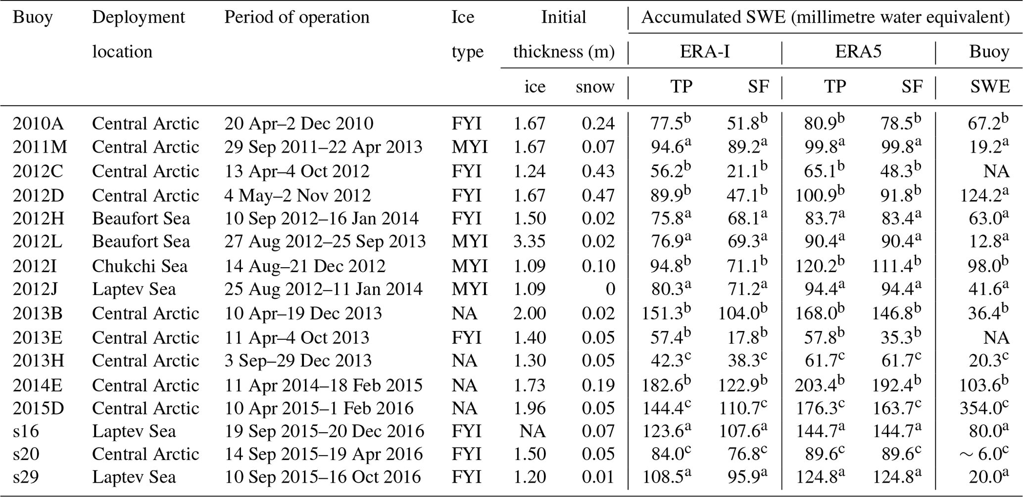
NA: no data. ^a From 1 October to 30 April. ^b Ice growth estimation by the end of freezing season with the Lebedev FDD model (Maykut, 1986). ^c From 1 October until the buoy fails or there are no longer snow data during the first freezing season.

Download Print Version | Download XLSX

2.2 ERA5 and ERA-I reanalysis data

ERA5 is the ECMWF's latest reanalysis product, and will replace the widely used ERA-I. The first series of ERA5, covering the period 2010–2016, was released in July 2017. The entire ERA5 dataset, extending back to 1950 will be available for use in late 2019. ERA5 and ERA-I both have global coverage, with a horizontal spatial resolution of 80 km for ERA-I and 31 km for ERA5. In the vertical, ERA5 resolves the atmosphere using 137 levels from the surface up to a height equalling 0.01 hPa, and ERA-I uses 60 levels from the surface up to an equivalent height of 0.1 hPa. ERA5 provides hourly analysis and forecast fields, while ERA-I provides 6-hourly analysis and 3-hourly forecast fields. For the data assimilation, both apply four-dimensional variational analysis (4D-var). ERA-I uses the Integrated Forecast System (IFS) “Cy31r2” 4D-var (https://www.ecmwf.int/en/forecasts/documentation-and-support/changes-ecmwf-model/ifs-documentation, last access: 17 March 2018), and ERA5 applies the newer IFS “Cy41r2” 4D-var. ERA5 includes various newly reprocessed datasets, for example, OSI-SAFr, the reprocessed version of the Ocean and Sea Ice Satellite Application Facilities (OSI-SAF) sea ice concentration (Hersbach and Dee, 2016), and recent instruments that could not be ingested in ERA-I. Many new parameters, such as 100 m wind vector, are available as part of the ERA5 output. For comparison and evaluation against buoy observations, ERA5 is bilinearly interpolated to the buoy positions, and ERA-I is first linearly interpolated to hourly data, and then bilinearly interpolated to the buoy positions. For comparison between ERA-I and ERA5 over the Arctic sea ice, the ERA-I data are first bilinearly interpolated to the grid of ERA5, and then T2M is averaged by season, and total precipitation and snowfall are integrated over the season.

3.1 Spatial distribution of seasonal differences of ERA5 and ERA-I near-surface temperature, snowfall and precipitation

Figure 2 shows the seasonal mean differences of T2M, total precipitation (TP) and snowfall (SF) between ERA5 and ERA-I over Arctic sea ice during 2010–2015. We classify spring as March, April and May, summer as June, July and August, autumn as September, October and November, and winter as December, January and February. The seasonal mean ice extent is obtained from the monthly sea ice concentration from NOAA/NSIDC during 2010–2015 (Meier et al., 2017).

Figure 2Seasonal mean difference between ERA5 and ERA-I (ERA5-ERA-I) for T2M (a–d), total precipitation (e–h) and snowfall (i–l) in spring (a, e, i), summer (b, f, j), autumn (c, g, k) and winter (d, h, l) over Arctic sea ice during 2010–2015.

Download

The difference in T2M between ERA5 and ERA-I varies with season (Fig. 2a–d). ERA5 is generally warmer (0–1.2 ^∘C) than ERA-I in spring and winter, and colder (0–0.6 ^∘C) than ERA-I during summer and autumn over Arctic sea ice. These temperature differences are smaller during summer, but substantial during the other seasons. Near the North Pole, ERA5 is warmer than ERA-I in summer, but colder than ERA-I in winter. Whether warmer or colder, the differences between ERA5 and ERA-I are small (±0.4 ^∘C) in this region.

ERA-I is known to be a relatively “dry” global reanalysis product in the Arctic compared with most other modern reanalyses (e.g. MERRA-2, CFSR and JRA-55) (Lindsay et al., 2014; Merkouriadi et al., 2017; Boisvert et al., 2018). The TP in ERA5 is typically less than 10 mm water equivalent higher than for ERA-I in all seasons over Arctic sea ice, with the exception of the Atlantic sector in autumn, winter and spring where TP in ERA5 can be up to 30 mm water equivalent larger (Fig. 2e, g, h). The patterns of seasonal TP over sea ice are very similar in ERA5 and ERA-I (Fig. S1 in the Supplement), and with the distinctly highest annual TP in the Atlantic sector (Fig. S2).

Snowfall is substantially higher in ERA5 than in ERA-I in all seasons (Fig. 2i–l), particularly in the Atlantic sector, where SF is up to 50 mm snow water equivalent (SWE) higher in the spring, autumn and winter seasons (Fig. 2i–l). In summer snowfall is much larger in ERA5 in the central and eastern Arctic (30–50 mm SWE higher) (Fig. 2j). Thus the differences in the snowfall between ERA5 and ERA-I are much larger than for TP in all seasons except winter (Fig. 2i–l vs. Fig. 2e–h; see also Fig. S2). The patterns of seasonal snowfall over sea ice are very similar in ERA5 and ERA-I (Fig. S1). Annual SF has increased all across the Arctic, more than TP, especially in the Atlantic sector (>100 mm) and eastern Arctic (Fig. S2).

3.2 Comparison of reanalysis near-surface temperature, snowfall and precipitation against buoy observations

Both ERA-I and ERA5 accurately capture the observed evolution of MSLP measured by each of the buoys (not shown). The hourly difference between the reanalysis MSLP and observations is no more than a few hectopascals. Excellent agreements between observed MSLP in the Arctic and earlier reanalyses have been shown in previous studies (e.g, Makshtas et al., 2007), demonstrating that MSLP is well simulated in reanalyses. In the following, we will focus on near-surface temperature, snowfall and total precipitation.

3.2.1 Evaluation of near-surface temperature in ERA5 and ERA-I using buoy observations

Figures 3–4 and S3–S5 show time series of T2M from different buoys, the corresponding T2M difference between ERA5 and ERA-I, and T2M differences between reanalyses and observations at the buoys' positions. The observed T2M reveals the pronounced seasonal cycle in the Arctic. Low temperatures persist through winter and spring, before approaching 0 ^∘C in late May or early June. Temperatures near 0 ^∘C, or occasionally over 0 ^∘C, continue during summer, before lower temperatures return in late August or early September and decrease further in autumn.

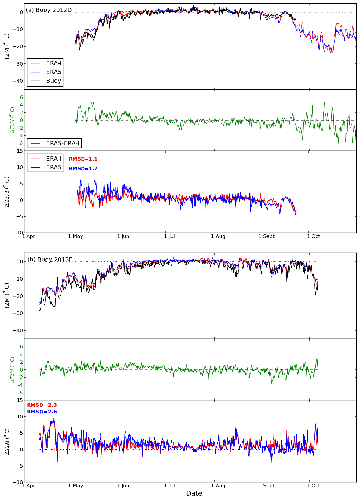
Figure 3Variation in 2 m air temperature (T2M) in ERA5, ERA-I, and the buoys (upper panel) and the differences of T2M between ERA5 and ERA-I (mid-panel; green) and comparisons for ERA5 and ERA-I with buoys (ERA5 minus buoy; ERA-I minus buoy) for buoys (a) 2012D and (b) 2013E. RMSD values for the comparison between ERA products and buoys are shown as text, blue for ERA5-buoy, red for ERA-I-buoy.

Download

Figure 4Same as Fig. 3, but for (a) buoy 2011M and (b) buoy 2012H.

Download

Table 2The mean T2M, accumulated FDD and estimated ice growth with the FDD model.

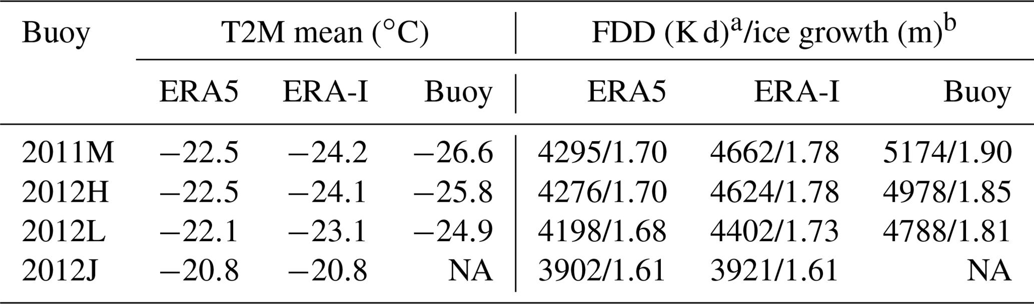
NA: no data. ^a From 1 October to 30 April. ^b Ice growth estimation by the end of freezing season with the Lebedev FDD model (Maykut, 1986).

Download Print Version | Download XLSX

The T2M in ERA5 and ERA-I generally agree well, both with each other and the observations (Figs. 3–4 and S3–S5). The reanalyses perform best for buoys 2013E (Fig. 3b) and 2012J (Fig. S5a), which were both deployed in the central Arctic, the former near the North Pole and the latter closer to the Laptev Sea (Fig. 1). On occasion, hourly differences of T2M between ERA5 and ERA-I can exceed 4 ^∘C (e.g. Fig. 4). The largest hourly T2M differences between the two reanalyses and between the reanalyses and observations (Figs. 3–4 and S3–S5) are found during the coldest months (November–May). Specifically, both reanalyses have a warm bias during these months. Previous studies have shown that warm biases in the Arctic are prevalent among most reanalysis products, particularly during the winter season (Beesley et al., 2000; Tjernstöm and Graversen, 2009; Lüpkes et al., 2010; Jacobson et al., 2012; Lindsay et al., 2014; Wesslén et al., 2014; Graham et al., 2017b). This is because weather forecast models and climate models struggle to accurately simulate strong stable boundary layers (Beesley et al., 2000; Tjernstöm and Graversen, 2009; Sotiropoulou et al., 2015; Graham et al., 2017b; Kayser et al., 2017; Biosvert et al., 2018). Interestingly, we find a larger warm bias in the new ERA5 compared with ERA-I (Figs. 3–4 and S3–S5, Table 2), despite the higher vertical resolution in ERA5. The root-mean-square deviation (RMSD) values are higher for ERA5 than for ERA-I (see Figs. 3–4 and S3–S5), in the range of 1.1–3.7 ^∘C for ERA-I and 1.7–4.6 ^∘C for ERA5.

We note that the near-surface air temperature in both reanalyses corresponds to a height of 2 m, while it is likely often measured by buoys at a lower height. The initial observation height might also decrease further as snow accumulates. During winter, the lowest temperatures in the Arctic occur under stable conditions with a strong surface-based inversion, meaning that the temperature increases with height from the surface. Hence, the near-surface warm bias in reanalyses may partly be attributed to the difference in height with the observations (Vihma et al., 2014). A prescribed ice thickness of 1.5 m and no snow accumulation on top of sea ice were applied in both ERA5 and ERA-I. The misrepresentation of snow may affect the surface energy budget, physically leading to, for example, overestimated conductive heat flux from the ocean to the surface.

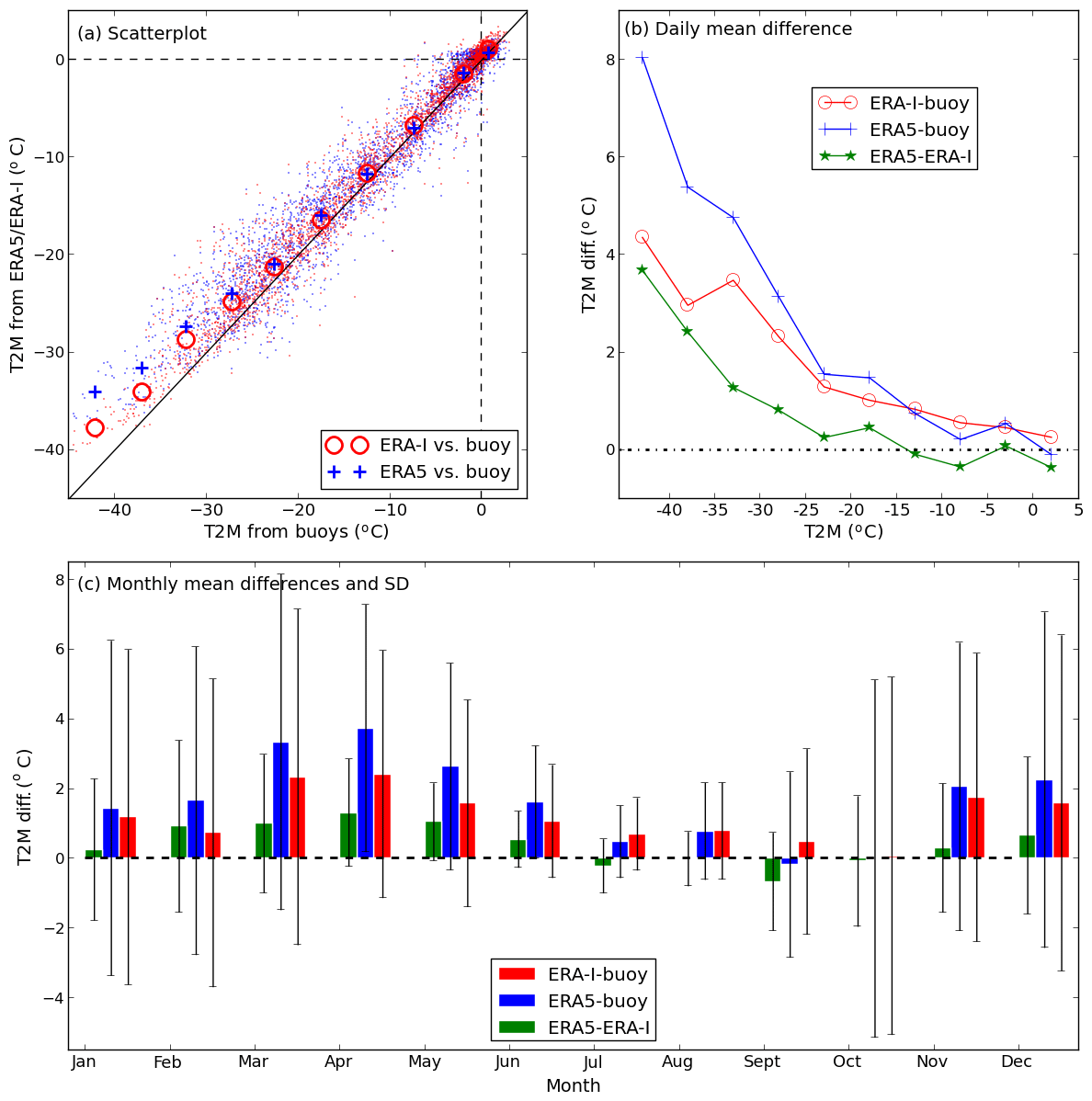
Figure 5Statistics of T2M from ERA5, ERA-I and all the buoys. (a) Scatter plot for all data (small dots) and average T2M at 5^∘ bins between −45 and +5 ^∘C, (b) daily temperature differences between the reanalysis and between the reanalysis and the buoys corresponding to 5^∘ bins between −45 and +5 ^∘C, and (c) monthly mean differences and standard deviation (SD). In panel (a), the black solid line is for 1 : 1.

Download

A scatterplot of ERA5–ERA-I vs. buoy T2M clearly reveals the temperature dependence of the warm bias in both reanalyses (Fig. 5a). The data crowd together near the 1 : 1 line when the air temperature is near 0 ^∘C, but spread further above the 1 : 1 line when the air temperature is low, especially at air temperatures below −25 ^∘C. The temperature dependence of the warm bias is also demonstrated in Fig. 5b, which shows the relationship between the daily mean T2M differences with the temperature bins of 5 ^∘C from −45 to +5 ^∘C. When the T2M is below −25 ^∘C, the daily mean difference between reanalysis and observation is higher than 2 ^∘C, with ERA5 3.1–8.0 ^∘C warmer than in buoys, and ERA-I 2.4–4.4 ^∘C warmer than in buoys (Fig. 5b). For air temperatures above −25 ^∘C, the bias between reanalysis and buoys is smaller, with ERA5 and ERA-I both 0.75 ^∘C warmer than the observations on average.

Figure 5c shows the bias and standard deviation (SD) for the reanalyses for each month, based on the buoy observations, and the temperature difference between the reanalyses. The smallest biases, and the smallest T2M differences between ERA5 and ERA-I are found in the months between July and October (also refer to Figs. 3–4 and S3–S5). ERA5 is typically warmer than ERA-I (and has a larger warm bias) throughout the winter and spring, including June. However, ERA5 is colder than ERA-I (0.01–0.6 ^∘C) and has a smaller bias from July to October (Fig. 5c). Hence, the warm bias in ERA5 is smaller than ERA-I in the warm season (July–October). ERA-I has a warm bias in the warm season, but the magnitude is smaller (<0.8 ^∘C) than the warm bias in the cold season (Fig. 5c). Similarly, ERA5 has a small warm bias during July and August (<1 ^∘C), and a likely insignificant cold bias (<0.2 ^∘C) in September and October (Fig. 5c).

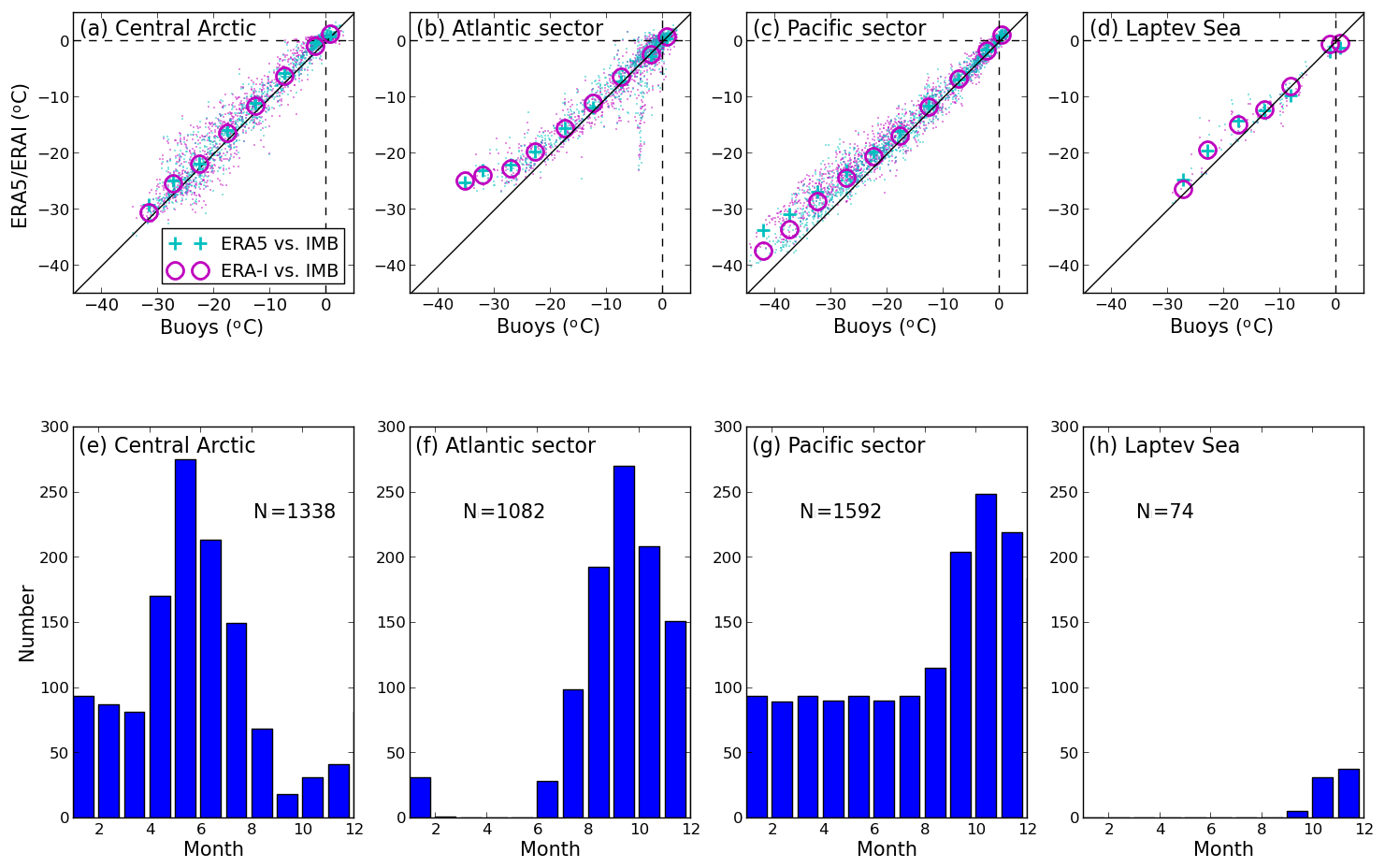
Figure 6Scatter plot of T2M from ERA5 and ERA-I vs. from buoys for the (a) central Arctic, (b) Atlantic sector, (c) Pacific sector, and (d) Laptev Sea, and number of buoy data (daily) per month for the (e) central Arctic, (f) Atlantic sector, (g) Pacific sector, and (h) Laptev sea. The definition of sectors are shown in Fig. 1.

Download

The performance of reanalysis near-surface temperature varies with region over Arctic sea ice (Fig. 6; also refer to Fig. 2). According to the buoys' positions (Fig. 1), we define four regions in the Arctic: the central Arctic (north of 86^∘ N), and the Pacific sector (90^∘ W–150^∘ E), the Atlantic sector (30^∘ W–60^∘ E), and the Laptev Sea (60–150^∘ E). The last three sectors are south of 86^∘ N. The ERA5 and ERA-I near-surface temperature performs best in the central Arctic (Fig. 6a), and well in the Pacific sector (Fig. 6c). It performs well in the Atlantic sector when the T2M is above −25 ^∘C, but poorly when the T2M is below −25 ^∘C (Fig. 6b). The performance of reanalysis near-surface temperature in the Laptev Sea needs to be further investigated due to a small number of observations in this region (Fig. 6d and h). However, there is also some seasonal bias in the availability of data from buoys in the different regions, largely due to when buoys are deployed in different regions of the Arctic and subsequent ice drift patterns.

3.2.2 Comparison of precipitation and snowfall from ERA5 and ERA-I along buoy drift trajectories

We next compare the cumulative total precipitation and snowfall in ERA5 and ERA-I in autumn and winter, along the drift trajectories of the buoys. We begin accumulation from 15 August onwards if the buoy was deployed before this date, or from 1 October if the buoy was installed after 15 August but before 1 October. We accumulate the precipitation until 30 April, or until the buoy stopped working if this occurred before 30 April (Table 1).

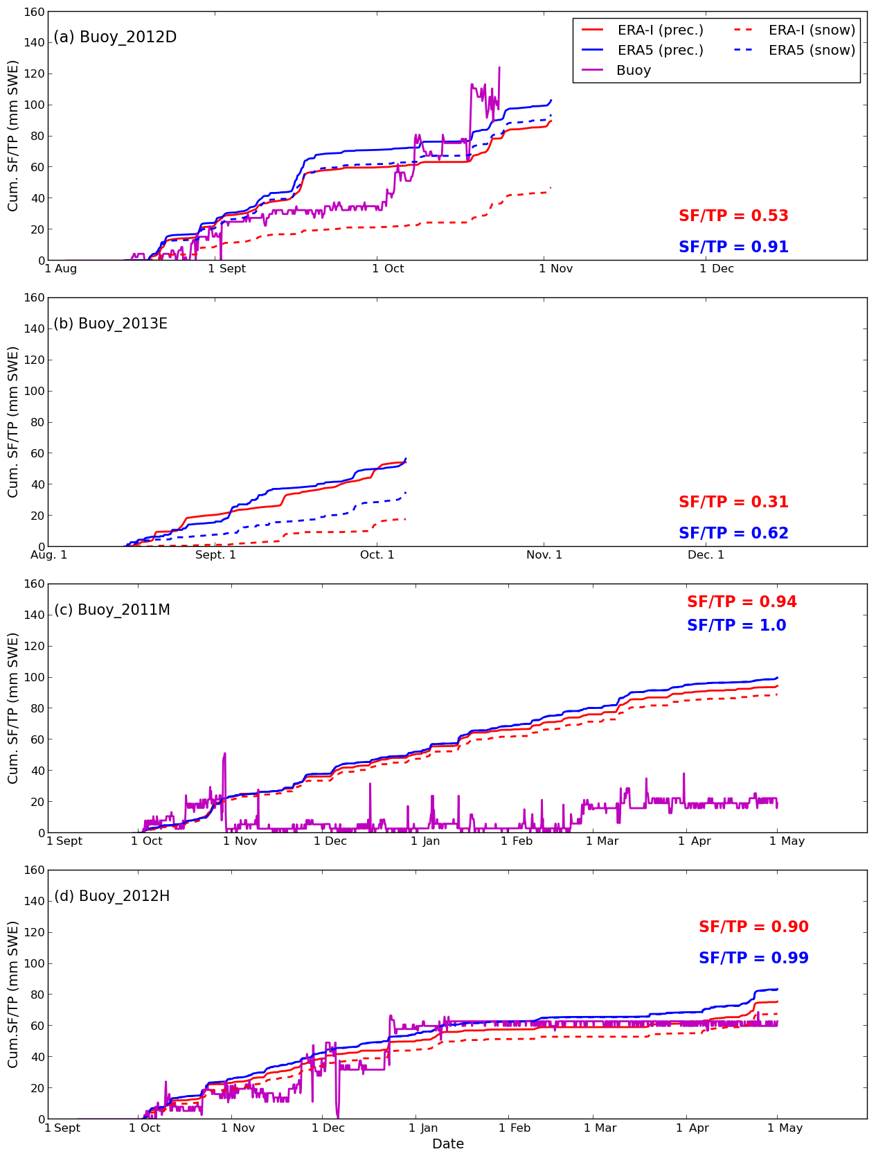
Figure 7Cumulative total precipitation (TP) and snowfall (SF) for ERA5 and ERA-I and snow depth for buoys (a) 2012D, (b) 2013E, (c) 2011M and (d) 2012H. Accumulation starts from 15 August for panels (a) and (b) and from 1 October for panels (c) and (d). The ratio of snowfall to total precipitation (SF ∕ TP) in ERA5 (blue text) and ERA-I (red text) is also shown in the figure. Note there were no snow depth data for buoy 2013E during the accumulation period.

Download

The accumulated total precipitation (TP) in ERA5 is higher than ERA-I for all buoys (Figs. 7 and S6–S7, and Table 1), which is consistent with the seasonal difference in TP documented in Sect. 3.1 (Fig. 2e–h). On average, the accumulated TP in ERA5 is 13.8 mm water equivalent larger than in ERA-I, with differences for the individual buoys ranging from 0.4 (buoy 2013E; Fig. 7b) to 31.9 mm water equivalent (buoy 2012D; Fig. 7a). This is in agreement with the seasonal differences between the reanalyses (Fig. 2e–h).

Similar to the accumulated TP, the accumulated snowfall (SF) in ERA5 is larger than in ERA-I (Figs. 7 and S6–S7; Table 1). For buoys deployed near the North Pole that started accumulating on 15 August, the accumulated SF in ERA5 is typically much larger than for ERA-I (Figs. 7a–b and S6, S7a). In contrast, for buoys deployed in other regions, which started accumulating on 1 October, the accumulated SF in ERA5 is typically slightly higher than ERA-I (Figs. 7c–d and S7b–f).

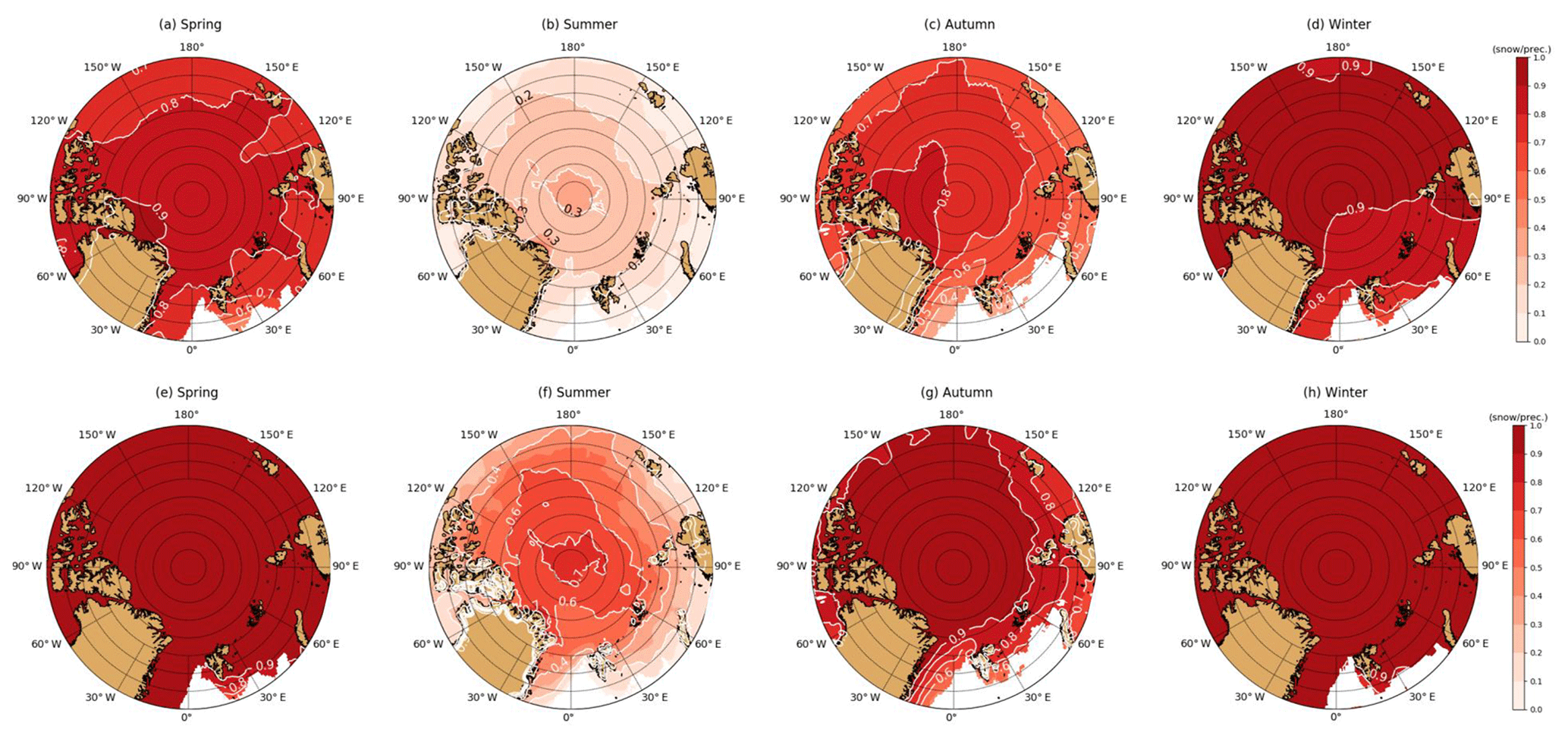
Figure 8The ratio of snowfall to total precipitation (SF ∕ TP) in ERA-I (a–d) and ERA5 (e–h) in spring (a, e), summer (b, f), autumn (c, g) and winter (d, h).

Download

The ratio of snowfall to total precipitation (SF ∕ TP) in ERA5 and ERA-I along the buoy trajectories is shown in Figs. 7 and S4–S5. A higher ratio means that more precipitation falls as snow. The ratio of SF ∕ TP for the buoy trajectories ranges from 0.31 to 0.94 in ERA-I, and from 0.62 to 1.0 in ERA5, with consistently more precipitation falling as snow in ERA5. The SF ∕ TP ratio for ERA5 increases on average by 0.28 for the buoys that started accumulating on 15 August compared with that in ERA-I. In contrast, the ratio of SF ∕ TP is usually 0.1 higher in ERA5 than in ERA-I for buoys that started accumulating on 1 October. This means that a substantial fraction of precipitation falls as rain in ERA-I during autumn (August–September), but the same precipitation events in ERA5 are classified as snowfall. This difference in SF ∕ TP ratio can help to explain why the accumulated SF in ERA5 is much greater than ERA-I for buoys deployed in August, but only slightly higher than ERA-I for buoys starting in October. The higher ratio of SF ∕ TP in ERA5 than in ERA-I takes place in all seasons over the Arctic sea ice (Fig. 8a–d vs. Fig. 8e–h). The increase in SF ∕ TP ratio in ERA5 is more significant in autumn (∼0.2) and summer (∼0.3–0.4) along the buoy trajectories, and relatively small in winter (∼0.1) and spring (∼0.1–0.2). This indicates more precipitation falls as snow in ERA5 not only in autumn but also in summer.

The low SF ∕ TP ratio and thus larger fraction of rainfall in ERA-I is known to be anomalous, and is likely due to the cloud physics scheme used (e.g. Dutra et al., 2011; Leeuw et al., 2015). In ERA-I, the split between liquid and ice in clouds is determined diagnostically as a function of temperature from −23 to 0 ^∘C, with ice only below −23 ^∘C and liquid only above 0 ^∘C. In contrast, the IFS Cy41r2 used in ERA5 includes a prognostic microphysics scheme, with separate cloud liquid, cloud ice, rain and snow prognostic variables (Sotiropoulou et al., 2015; see also ECMWF IFS documentation – Cy41r2; https://www.ecmwf.int/sites/default/files/elibrary/2016/16648-part-iv-physical-processes.pdf, last access: 4 March 2019). Our findings indicate that ERA5 has significantly less Arctic rainfall than ERA-I, particularly in autumn (Figs. 7, S6–S7) and summer (Fig. 8b and f).

Evaluating the performance of precipitation products over the Arctic Ocean is a major challenge due to the lack of observations, and difficulty accurately measuring snowfall (e.g. Lindsay et al., 2014; Rasmussen et al., 2012; Sato et al., 2017; Blanchard-Wrigglesworth et al., 2018; Boisvert et al., 2018; Webster et al., 2018). Here we compare the precipitation from ERA-I and ERA5 with snow depth measurements from the buoys (Table 1). For this comparison, snow depth from the buoys is converted to snow water equivalent (SWE) using a climatological monthly mean snow density of 220–380 kg m⁻³ (Warren et al., 1999). Caution must be taken here, as the buoys reflect point observations, while the reanalyses provide a grid cell average. Snow depth is known to have large variability even over relatively small spatial scales (Warren et al., 1999; Sturm et al., 2002; Liston et al., 2018). An unknown fraction of the true snowfall will also be lost through blowing snow into leads, which is not accounted for in our calculation.

The accumulated TP and SF from ERA-I and ERA5 are generally comparable with the observed SWE from buoys in most cases during the accumulation period (refer to Figs. 7 and S6–S7), such as for buoy 2012H deployed in the Beaufort Sea (Fig. 7d). However, in several cases the accumulated TP and SF from ERA-I and ERA5 are considerably lower than the observed SWE from buoys, such as for buoy 2012D from mid-September (Fig. 7a). This may be caused by snow drifting up against the buoy structure, or reflect anomalously low precipitation in the reanalyses. In other cases, the accumulated TP and SF from reanalysis is higher than the observed SWE from buoys during some periods [buoys 2013B (Fig. S6c) and s20 (Fig. S7e)] or for the whole accumulation period [buoys 2011M (Fig. 7c), 2012L (Fig. 7c) and S29 (Fig. S7f)]. This could be caused by snow erosion/sublimation around the buoy, or reflect anomalously high precipitation in the reanalyses. By the end of the accumulation period, the accumulated TP (SF) is larger on average by 55.4 mm (41.9 mm) SWE for ERA-I and 66.5 mm (62.8 mm) SWE for ERA5 than the observed SWE of the snowpack along the buoy trajectories (see Table 1).

4.1 Assessing the sea ice evolution with freezing degree days (FDDs): impact of temperature bias

The cumulative freezing degree days (FDDs) model only needs air temperature as input and is often used to estimate sea ice growth (Δh) from zero (e.g. Huntemann et al., 2014; Lei et al., 2017). The sea ice growth is estimated based on Lebedev (Maykut, 1986), $\mathrm{\Delta }h=\mathrm{1.33}\sum {\left(\mathrm{FDD}\right)}^{\mathrm{0.58}}$, where ∑FDD is daily average temperature below the freezing point of sea water (−1.8 ^∘C), integrated over the time period from 1 October to 30 April.

The positive near-surface air temperature bias in ERA5 and ERA-I results in a negative ice thickness bias at the end of the growth season. The cumulative FDD is smallest for ERA5 (Fig. S8, Table 2), corresponding to the largest warm bias in ERA5 during the freezing season. The differences in FDD between ERA5, ERA-I and buoys are large for buoys 2011M, 2012H and 2012L, but negligible for buoy 2012J. The ice growth is 0.08–0.12 m less, with a mean of −0.09 m for ERA-I T2M, and 0.13–0.20 m less, with a mean of −0.16 m for ERA5 T2M compared to when using near-surface buoy temperatures (Table 2).

4.2 Assessing sea ice evolution with a 1-D sea ice model HIGHTSI: impact of T2M and precipitation

HIGHTSI is a 1-D high-resolution thermodynamic snow and ice model designed for process studies to resolve the evolution of snow–ice thickness and temperature profile. The snow and ice temperature regimes are solved by the partial differential heat conduction equations applied for snow and ice layers, respectively. The turbulent surface fluxes are parameterized taking the thermal stratification of the atmosphere surface layer into account. Downward short- and longwave radiative fluxes are parameterized based on the total cloud cover. The model has been extensively used in Arctic studies (e.g. Cheng et al., 2008, 2013; Wang et al., 2015; Merkouriadi et al., 2017).

In this section we perform six sensitivity simulations on each of the four buoys to explore the impact of temperature and precipitation on snow and sea ice evolution (Table 3). In the first two simulations, SFI_T2MI and SF5_T2M5, we force HIGHTSI with the T2M, 10 m wind speed (V), relative humidity (RH), total cloud cover (CN) and snowfall, from ERA-I and ERA5 (Fig. S9), respectively. In the next two simulations, TPI_T2MI and TP5_T2M5, we force the model with the total precipitation from the reanalyses, rather than the snowfall, and treat precipitation as snow only when T2M is below 0 ^∘C. In the final two simulations, we evaluate the influences of T2M and precipitation on the sea ice evolution individually. Specifically, we replace the T2M from ERA-I in the TPI_T2MI run with the T2M from ERA5, and name this run TPI_T2M5. Similarly, we replace the TP from ERA-I, in the run of TPI_T2MI, with the TP from ERA5 for the TP5_T2MI run (see Table 3). For all of the simulations we apply a seasonally variant ocean heat flux according to McPhee et al. (2003), which is large in October (10–20 W m⁻²) and decreases to nearly zero from mid-November (see Fig. S9). Snow ice, an ice type formed at ice surface (e.g. Leppäranta, 1983), was recently found to significantly contribute to the Arctic sea ice mass balance in a region with thick snowpack on relatively thin ice (Granskog et al., 2017; Merkouriadi et al., 2017). A few (1.5–3) millimetres of snow ice formed only in the TPI_T2MI and TPI_T2M5 runs for buoy 2012J (with the lowest initial ice thickness of all buoys examined, Table 1). This is negligible for the total ice mass balance. Thus, the effect we examine solely depends on the differences in T2M and precipitation–snowfall on thermodynamic ice growth.

Table 3Model runs and atmospheric forcing data in model simulations, where TP is total precipitation, SF is snowfall, V is wind at 10 m height, RH is relative humidity and CN is total cloud cover.

Download Print Version | Download XLSX

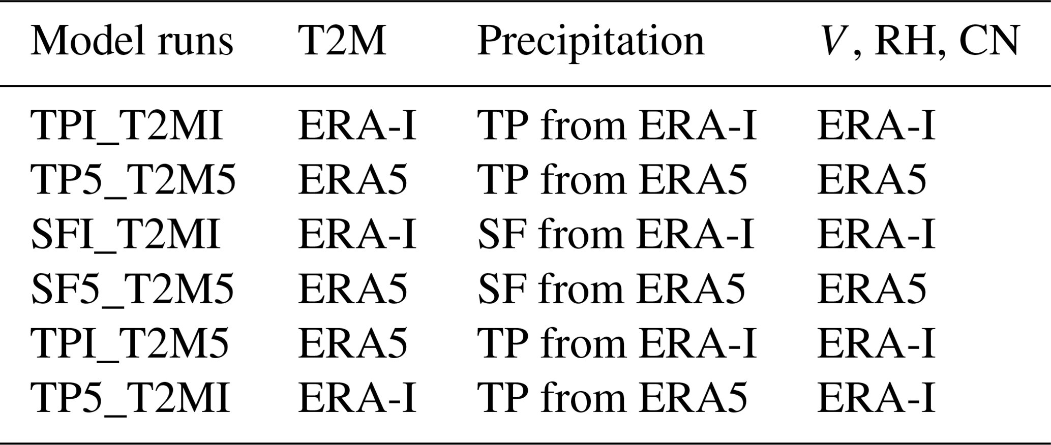
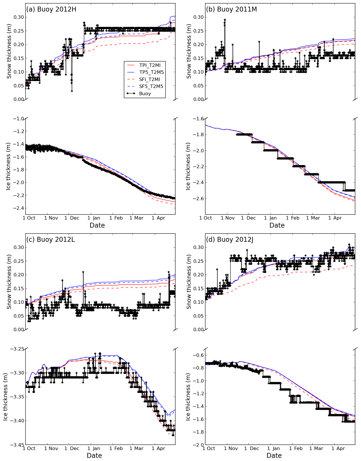
Figure 9Evolution of snow and sea ice thickness during the freezing season based on simulations with HIGHTSI for (a) buoy 2012H, (b) buoy 2011M, (c) buoy 2012L and (d) buoy 2012J for runs TPI_T2MI, TP5_T2M5, SFI_T2MI and SF5_T2M5.

Download

The pattern of snow accumulation recorded by many buoys is consistent with observations by Warren et al. (1999). Namely, they record snow accumulation in late autumn, followed by a relatively constant snow depth from December–January to March, and sometimes a late increase in snow depth in early spring (Fig. 9). For example, the observed snow depth at buoy 2012H increased to about 0.25 m in late December, and changed marginally thereafter (Fig. 9a). Similarly, the observed snow depth at buoy 2012L increased from 0.03 to 0.13 m from early October to mid-November, and then remained around 0.10 m until the end of April (Fig. 9c). The buoys sooner or later recorded an increase in ice thickness during the freezing–growth season. For example, the sea ice growth for buoy 2012H began in early December, at a rate of approximately 0.5 cm d⁻¹, until late March, and afterward the growth became sluggish at a rate of 0.16 cm d⁻¹ until the end of April (Fig. 9a). However, buoy 2012L, which had an initial ice thickness of ∼3.3 m, showed no significant growth until early February, before undergoing a slight increase from around 3.3 to 3.42 m by the end of the freezing season (Fig. 9c). Sea ice growth for buoy 2011M (Fig. 9b) and 2012J (Fig. 9d) showed a staircase pattern since the ice thickness was derived from measured temperature profile due to the failure of acoustic sounders as mentioned in Sect. 2.1.

We first compare the simulations TPI_T2MI and TP5_T2M5. Differences in the ice thickness at the end of the growth season for these simulations are relatively small, despite the larger warm bias in ERA5 (Fig. 9). Sea ice was marginally thinner (0.006–0.02 m) in TP5_T2M5 compared with TPI_T2MI for all the buoys. The major differences we see between these simulations is in the snow depth (Fig. 9). TPI_T2MI has a thinner snowpack than TP5_T2M5 for all four buoys, by 0.02–0.06 m. This is due to the higher total precipitation in ERA5, compared with ERA-I (see Sect. 3.2).

In contrast, when HIGHTSI is forced with the reanalysis' snowfall product (SFI_ERAI and SF5_ERA5) the differences in snow depth are comparable with the simulations forced by the total precipitation (TPI_T2MI and TP5_T2M5). The SFI_T2MI runs typically have a thinner snowpack (0.01–0.06 m) and a greater ice thickness (0.04–0.09 m) than SF5_T2M5. The snow depth in SFI_T2MI is thinner (by 0.01–0.04 m) and ice thickness is greater (0.01–0.06 m) than the TPI_T2MI runs (Fig. 9). This is because there is substantial rain at sub-zero temperatures in the SFI_T2MI runs that is classified as snow in the TPI_T2MI runs. There are no large differences between the snow depth and sea ice thickness at the end of the growth season for the SF5_T2M5 and TP5_T2M5 runs because, unlike in ERA-I, there is little rain at sub-zero temperatures for SF5_T2M5.

Figure 10Same as Fig. 9, but for model runs TPI_T2M5 and TP5_T2MI.

Download

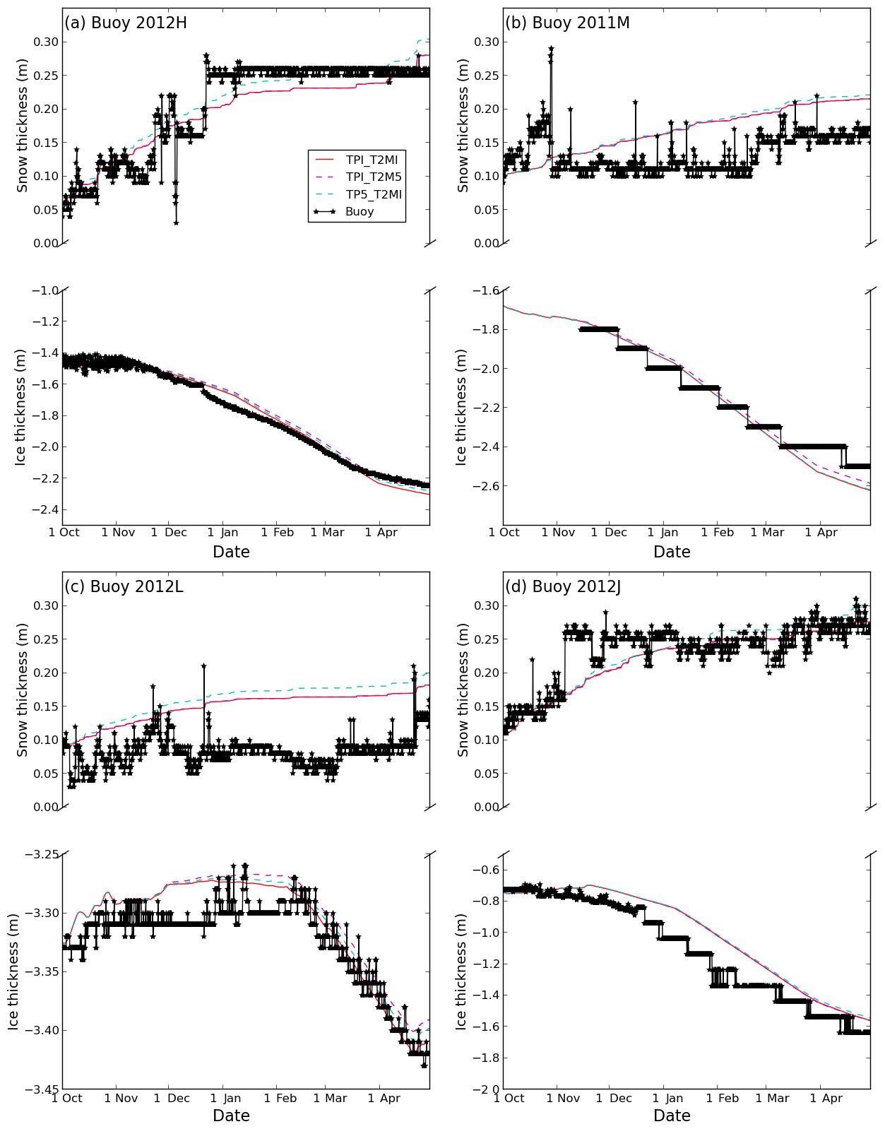
We now look at the effect of T2M differences between ERA5 and ERA-I, and compare the TPI_T2M5 runs vs. TPI_T2MI runs (Fig. 10). When using the T2M from ERA5 and not altering the precipitation forcing, the snowpack remains unchanged from the TPI_T2MI run. However, we find a slightly thinner ice at the end of the freezing season, compared with TPI_T2MI runs (0–0.04 m thinner), as a result of the larger warm bias in ERA5, which slows down the growth of sea ice. This is consistent with our results from the FDD model in Sect. 4.1.

Finally, we look at the effect of precipitation by comparing the TP5_T2MI and TPI_T2MI runs. The snowpack in TP5_T2MI is thicker (0.006–0.02 m), while the ice thickness is thinner (0.003–0.02 m) than in the TPI_T2MI runs (Fig. 10). The thicker snowpack is due to the higher precipitation in ERA5 compared with ERA-I. This thicker snowpack allows less heat loss to the atmosphere, which results in less ice growth.

Overall the difference of using different T2M and TP forcings is very moderate and equal in magnitude during the freezing period. Obviously using the ERA-I SF will result in larger differences, due to the low SF in ERA-I.

In general, HIGHTSI reproduces the evolution of snow and sea ice observed by the buoys well during the freezing season (Figs. 9–10) although there are some differences. For the snowpack, there was a 10 cm increase in snow depth for IMB_2012H during late December, which seems not well captured by any of the reanalyses and therefore by any of the simulations (Figs. 9a and 10a). The simulations for IMB_2012H show an increase in snow depth at the end of April, indicating a snowfall event in the reanalysis. However, this was not recorded by the buoy. Thus, not only the magnitude but also the frequency of the precipitation in the reanalysis data are crucial for the snow evolution in the simulation. The representation of snow in the model may further influence the simulated ice thickness (e.g. Fig. 9a). Evaluating precipitation in the Arctic is however challenging as mentioned previously due to the large local variability and lack of representative in situ observations (e.g. Liston et al., 2018). Differences in the modelled sea ice thickness from the buoy observations in part arise from not knowing the local ocean heat flux at each individual buoy; however, our approach is to look at the sensitivity relative to the differences in T2M and precipitation–snowfall in the reanalyses.