2.1 Sea ice albedo scheme of HIRHAM–NAOSIM

The most recent version of the coupled regional climate model HIRHAM–NAOSIM consists of the atmosphere component HIRHAM5 and the ocean–sea ice component NAOSIM in its fine-resolution version. A detailed model description is given by Dorn et al. (2018). Using a regional model with focus on the Arctic allows an improved description of Arctic processes and feedbacks between atmosphere, sea ice, and ocean (Rinke et al., 2013). However, as stated by Køltzow (2007), the model sensitivity to changes in the SIS albedo parameterization would be higher in such coupled climate models, which may lead to larger uncertainties.

The latest version of the SIS albedo scheme applied in HIRHAM–NAOSIM is described by Dorn et al. (2009). Here only the essential equations are presented, which are directly applied to the measured data set. For an inhomogeneous surface, the surface albedo in a model grid cell can be considered a sum of the individual surface albedo values weighted by the areal fractions (c) of the respective surface subtypes:

with the subscript i indicating the sea ice types, and ow representing open water. Since the surface albedo of sea ice is highly variable compared to open water, which is assumed to be 0.1, the individual albedo of ice types needs to be classified in subtypes: snow-covered ice (subscript s), bare ice (subscript bi), and melt ponds (subscript m) following the parameterization of Køltzow (2007). This results in an overall SIS albedo calculated by

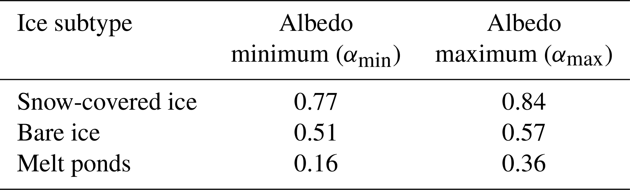
The albedo of the surface subtypes is variable due to their changing physical properties. In particular in the melting season, the surface reflection properties change on a daily basis depending on the surface temperature and snow depth. In the SIS albedo scheme applied in HIRHAM–NAOSIM, Dorn et al. (2009) estimated ranges of possible surface albedo values as shown in Table 1.

Table 1Minimum and maximum values of surface albedo of snow-covered ice, bare ice, and melt ponds as used in the SIS albedo scheme.

Download Print Version | Download XLSX

The parameterized surface albedo of the subtypes is determined by

with f(T_surf) representing the surface temperature-dependent function:

where T_surf and T_d are given in degrees Celsius. T_d describes a temperature threshold, where the surface albedo change of the subtypes is expected to be significant. In HIRHAM–NAOSIM the value of T_d is set to −0.01 ^∘C for snow-covered and bare ice, while for melt ponds T_d is estimated with −2 ^∘C (Dorn et al., 2009). This results in a sharp drop of albedo for bare ice and snow-covered ice from α_max to α_min between $T_{\mathrm{surf}}=-\mathrm{0.01}$ and 0.0 ^∘C, whereas for melt ponds a linear decrease in α_m between $T_{\mathrm{surf}}=-\mathrm{2.0}$ and 0.0 ^∘C is estimated.

After parameterization of the sea ice subtype surface albedo, their areal fractions according to Eq. (2) need to be retrieved to calculate the final SIS albedo of the model grid cell. The discrimination between bare ice and snow-covered sea ice is estimated by the prognostic variable snow thickness (h_s) in HIRHAM–NAOSIM. The parameterization of the snow cover fraction as presented by Dorn et al. (2009) reads

where c_s,max is the maximum snow cover fraction of 0.99 and h_0.75 gives the snow thickness at which 75 % of the sea ice is covered by snow, which is estimated with h_0.75=0.03 m. The melt pond fraction is parameterized by

as suggested by Køltzow (2007) with $c_{\mathrm{m},\max }=\mathrm{0.22}$ giving the maximum melt pond fraction. The limitation of the melt pond fraction prevents a complete conversion from snow to melt ponds when temperatures reach 0 ^∘C. The given value of 0.22 refers to SHEBA data derived from aerial imagery (Perovich et al., 2002). More recent data (see, e.g., Istomina et al., 2015) indicate that this value is too low, in particular for first-year ice that has become more important over the last years. Readjustment of c_m,max, for instance as a function of the sea ice age, is envisaged for follow-up studies. However, for the time frame of the ACLOUD campaign, the threshold of $c_{\mathrm{m},\max }=\mathrm{0.22}$ is appropriate.

The parameterized SIS albedo for a sea ice cover of 100 % is illustrated in Fig. 1a. It comprises the temperature dependence of the subtype's surface albedo (Eq. 3) and the melt pond fraction (Eq. 6), as well as the snow depth dependence of the surface fraction of snow-covered ice (Eq. 5). The significant gradient of the surface albedo around 0 ^∘C is mainly related to the choice of the small temperature range where the surface albedo of snow-covered ice and bare ice migrates from the maximum to the minimum value within ΔT_surf = 0.01 K. Outside the temperature range between threshold temperature T_d and 0.0 ^∘C, the parameterized SIS albedo is only dependent on the snow depth, which is directly linked to c_s. The change in the surface subtype fractions, exemplarily determined for −0.1 ^∘C, is shown in Fig. 1b. The bare ice fraction ($c_{\mathrm{bi}}=\mathrm{1}-c_{\mathrm{s}}-c_{\mathrm{m}}$) only dominates when snow depth values are lower than 0.01 m for this specific case. Together with Fig. 1a, it becomes obvious that the snow depth dependence of the surface subtype fraction becomes solely relevant for h_s<0.1 m.

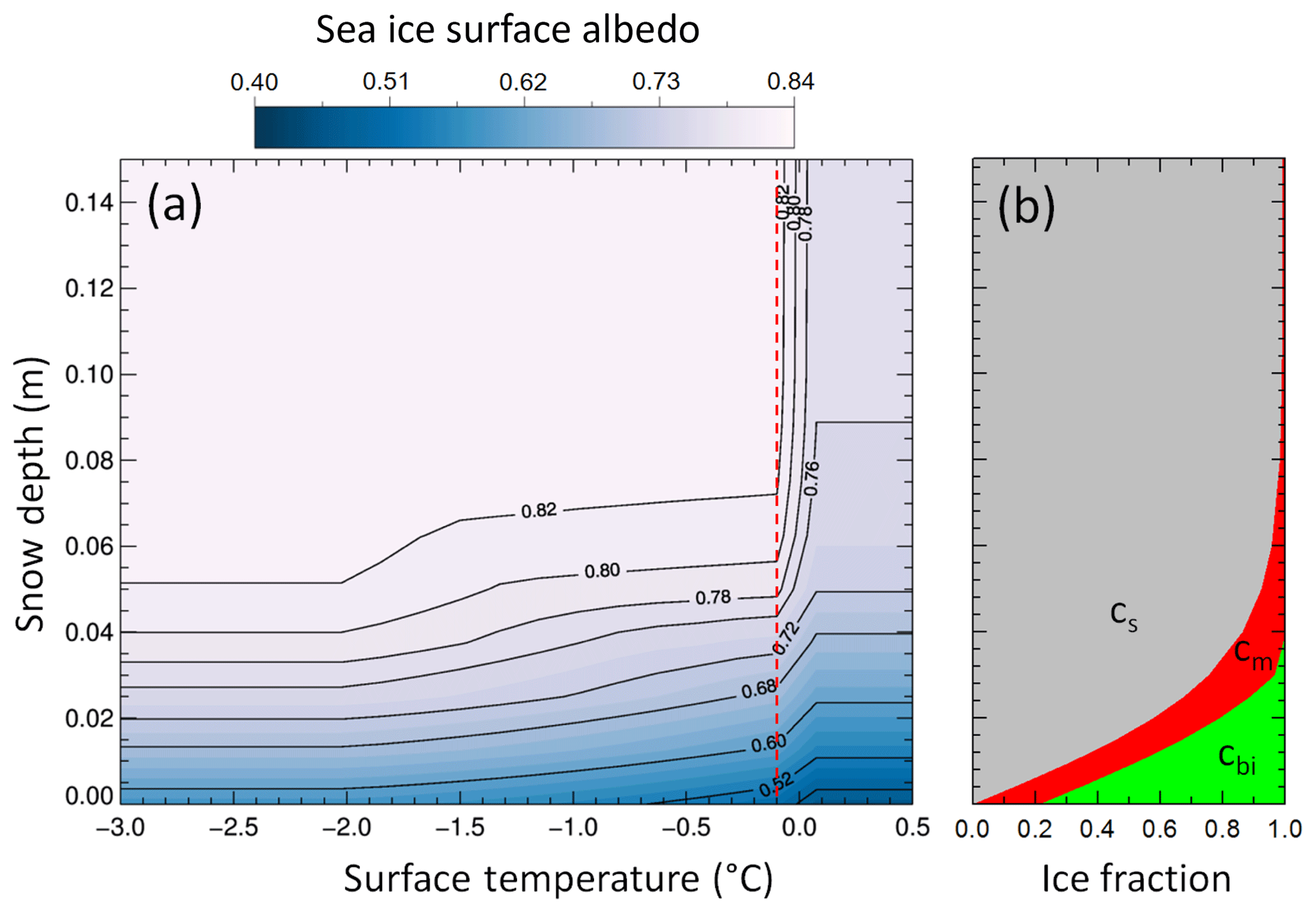
Figure 1(a) Contour plot of the SIS albedo dependent on snow depth and surface temperature as parameterized from the SIS albedo scheme of HIRHAM–NAOSIM for an area with 100 % sea ice cover. The vertical red-dotted line marks a surface temperature of −0.1 ^∘C, for which the surface subtype fractions are plotted in (b).

Download

2.2 Ground-based and aircraft observations

To test the SIS albedo scheme of the HIRHAM–NAOSIM model offline from the HIRHAM–NAOSIM output, measured values of the prognostic variables T_surf and h_s are used to calculate the SIS albedo and the individual fractions of the sea ice subtypes. The combined ACLOUD/PASCAL campaigns were conducted in May–June 2017 north of Svalbard as part of the (AC)³ project (Wendisch et al., 2017). During ACLOUD, airborne observations of cloud, aerosol particle, and surface properties were collected by the two research aircraft Polar 5 and Polar 6. In connection to the aircraft activities, during PASCAL ground-based measurements on a drifting ice floe station and shipborne observations with the research vessel (RV) Polarstern were conducted in close collocation to the aircraft. Also, a data set of the SIS albedo was sampled from buoy observations from the beginning of June to middle of July. An overview of the concurrent campaigns and a synoptic overview is given by Wendisch et al. (2018) and Knudsen et al. (2018), respectively. Three different synoptic periods were classified during ACLOUD/PASCAL, a cold period (23–29 May 2017), followed by a warm period (30 May to 12 June 2017), and a normal period (13–26 June 2017).

Suitable measurement cases for the validation of the SIS albedo scheme were selected based on the following restrictions: (i) flight altitude lower than 100 m to minimize atmospheric masking in the surface albedo from the aircraft, (ii) aircraft pitch and roll angle are in a range of ±4^∘, and (iii) no clouds between aircraft and surface. Applying these filters to the aircraft data, suitable flight sections on 14 flights were identified. The corresponding flight paths of these days from both aircraft are plotted in Fig. 2. The percentage sea ice concentration derived for 15 June 2017 from satellite observations by the Advanced Microwave Scanning Radiometer (AMSR) instrument (Spreen et al., 2008) is displayed in the background. As indicator of the variability of the sea ice concentration within the course of the campaign, the 75 % isolines for 27 May and 26 June are additionally plotted in gray and black. The most significant decrease in sea ice extension becomes obvious between 8 and 12^∘ longitude in the northwest of Svalbard. In May, the sea ice edge was far south in this region. Due to northerly winds, a southerly to southwesterly sea ice drift was observed. With the beginning of the warm period at the end of May, the southerly winds led to a northeastward ice drift (Wendisch et al., 2018). This specific area was mainly observed at the end of May by both aircraft and middle of June by the Polar 5 aircraft. However, most of the selected flights were conducted over regions with more than 80 % sea ice coverage.

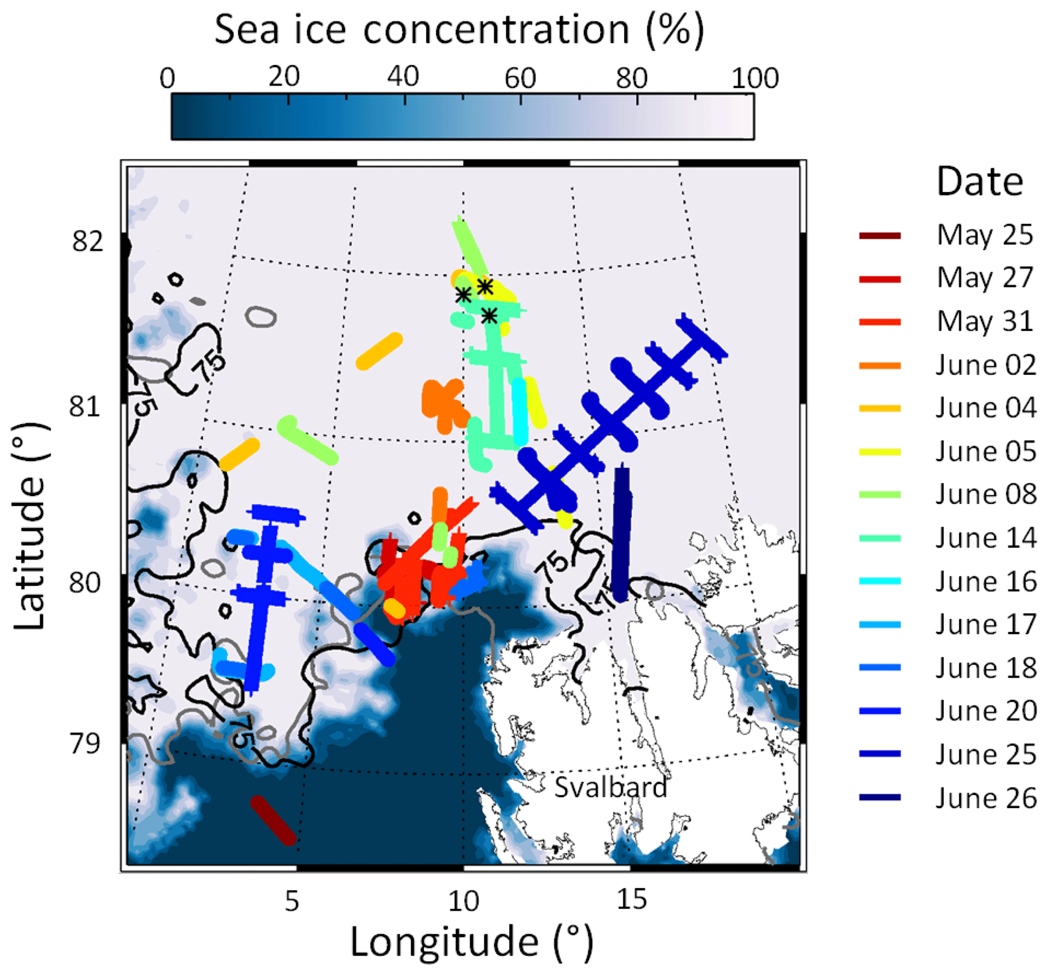
Figure 2Selected flight sections from Polar 5 and Polar 6 during ACLOUD/PASCAL (colored lines). The black stars indicate the area reached by the drifting ice floe between 5 and 14 June 2017. In the background, the sea ice concentration derived from satellite measurements (AMSR-sensor) for 15 June is shown. Additionally, the 75 % isolines of the sea ice concentration are plotted for 27 May (in gray) and 26 June (in black).

Download

During a 3-week period, snow depth was measured along a 3 km long transect (spatial resolution along track approx. 1 m) over the PASCAL sea ice floe using a Magna probe (Sturm and Holmgren, 2018). The temporal development of the daily snow depth frequency distribution along the transect is depicted in Fig. 3. The mean snow depth decreased rapidly in the course of the campaign as a result of melting in the warm period from 37±24 cm on 5 June to 22±18 cm on 14 June. Mostly relevant for the magnitude of snow albedo is a snow depth below 10 cm, where the albedo reveals an asymptotic increase with increasing snow depth (Grenfell and Perovich, 2004; Perovich, 2007). Considering only the percentage of measurements with h_s<10 cm revealed an increase in this fraction on the overall snow depth observations from 9 % on 5 June to 32 % on 14 June.

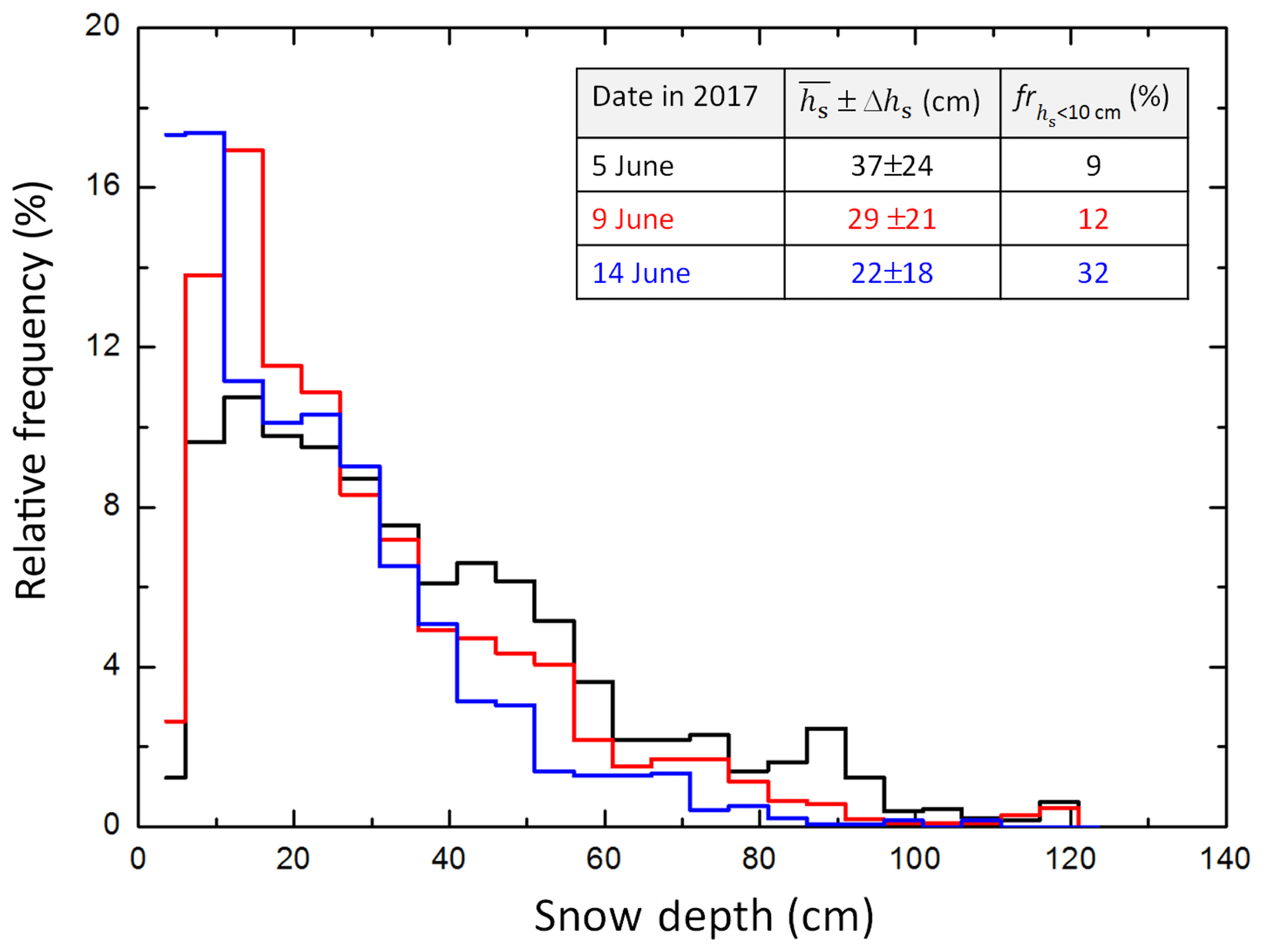
Figure 3Histogram of snow depth in centimeters measured by the Magna probe on the ice floe during PASCAL for different days of the period 5–14 June. Additionally, the mean snow depth and the standard deviation, as well as the fraction of measurements with a snow depth below 10 cm (fr${}_{h_{\mathrm{s}}<\mathrm{10}\mathrm{cm}}$), are given for each day.

Download

According to Eq. (3), surface temperature data are needed to apply the SIS albedo scheme of HIRHAM–NAOSIM. On board both aircraft, Polar 5 and Polar 6, a nadir-pointing infrared sensor (KT19.85; Wendisch et al., 2018) with a field of view of 2^∘ was installed to measure the brightness temperature of the surface along the flight track. The instrumental sensitivity covers parts of the atmospheric window between 9.6 and 11.5 µm wavelengths. Within this spectral range, the emissivity of snow and sea ice surfaces varies between 0.965 and 0.995 depending on snow type (Hori et al., 2006). The mean surface skin temperature and its standard deviation is shown for specific days in Fig. 4a. Since Polar 5 was mainly operated above the clouds, fewer days with suitable cases were found compared to the Polar 6 data set. The increase in surface temperature at the end of May indicates the change in the synoptic situation (Wendisch et al., 2018). In particular temperatures between −2 and 0 ^∘C in the middle of June represent a crucial range where the albedo of sea ice may change significantly, as considered in Eq. (4). The temporal development of the standard deviation in Fig. 4 shows that the variability of surface skin temperature caused by the contrast between warmer open water and colder sea ice along the individual flight tracks decreases with time.

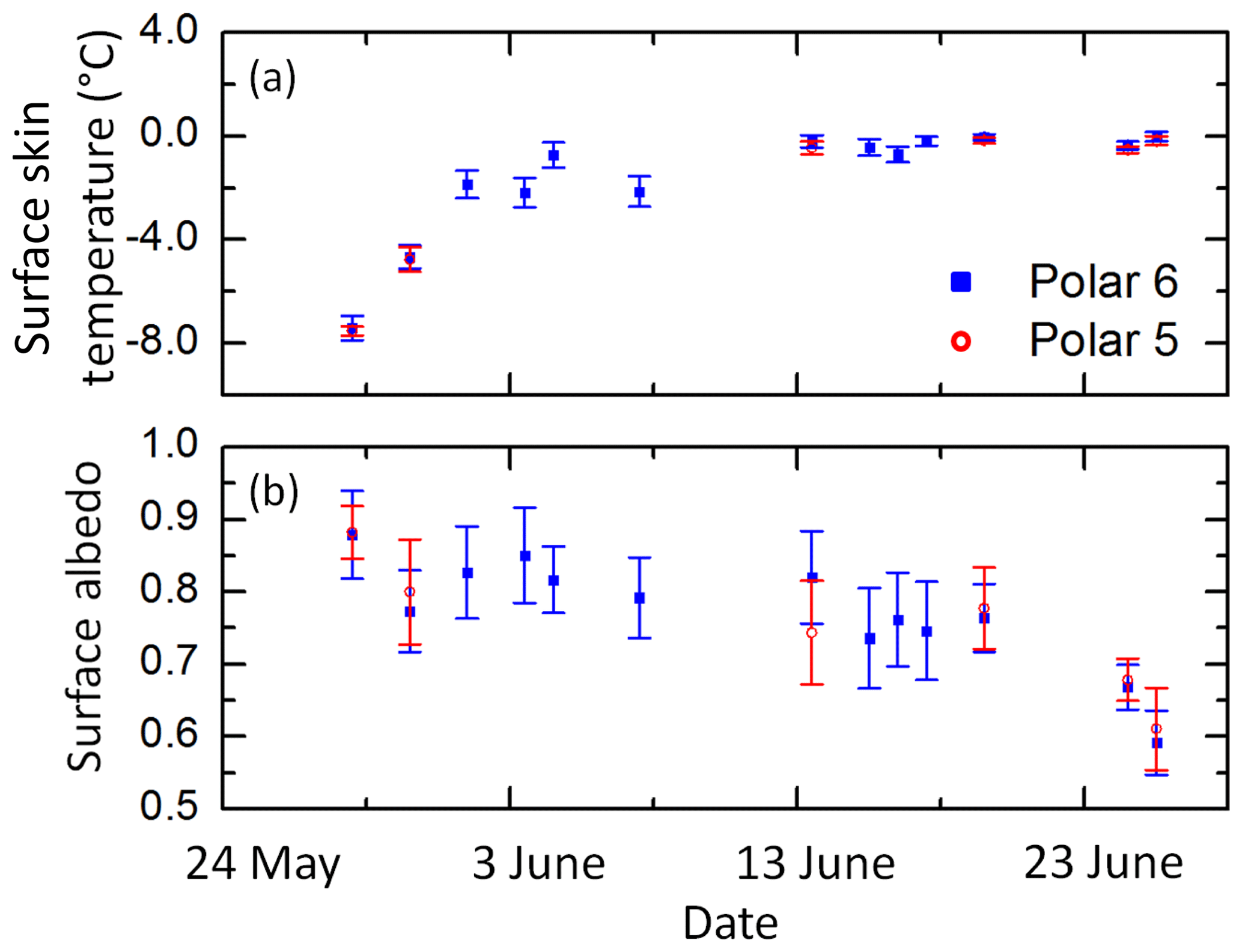
Figure 4(a) Mean surface skin temperature along flight tracks for selected days derived from KT19 measurements on board Polar 5 and Polar 6. (b) Corresponding mean albedo. The error bars give the standard deviation. The surface below the flight tracks was primarily snow-covered sea ice, but the measurements also consider locations with open water.

Download

The effect of the surface temperature increase on the surface albedo is directly evaluated using concurrent measurements of the surface albedo by upward- and downward-looking pyranometers. These pyranometers (Wendisch et al., 2018) were installed on both aircraft to sample the broadband solar irradiance between 0.2 and 3.6 µm wavelengths. The irradiance data were corrected for aircraft attitude (pitch and roll angle) following the techniques described by Bannehr and Schwiesow (1993). A deconvolution method was applied to the pyranometer measurements to enhance the temporal resolution (20 Hz) of the slow-response sensors (Ehrlich and Wendisch, 2015). The daily mean surface albedo along the selected flight sections as derived from the ratio of upward and downward irradiances is shown in Fig. 4b. As indicated by the range of the standard deviation, the spatial variability of the SIS albedo may have the same order of magnitude as the temporal variation. A broad range of ice surface albedo values is noticeable between the end of May (α=0.86) and the end of June (α<0.6) as was also shown by Wendisch et al. (2018) (see their Fig. 12). The clearly delayed decrease, caused by the temperature increase, indicates the transformation of sea ice properties.

The fractions of sea ice subtypes were documented by commercial digital cameras on both aircraft (Ehrlich et al., 2012; Wendisch et al., 2018). The cameras were equipped with a 180^∘ fisheye lens to observe the entire lower hemisphere with a spatial resolution of 3908×2600 pixels. Images were taken every 6 s. Laboratory calibrations of the cameras were performed with respect to their spectral, geometrical, and radiometrical properties. Subsequently, the raw signal for each image pixel was transferred to an absolute radiance value per viewing angle. Techniques to classify the surface types from remote-sensing imagery, in particular in Arctic regions, have been introduced by several authors (Perovich et al., 2002; Pedersen et al., 2009; Renner et al., 2013; Divine et al., 2015). In this study, the method of partitioning the image by manually selecting red, green, and blue (RGB) thresholds, based on color intensity histograms, is applied (Perovich et al., 2002). Depending on the illumination conditions, these thresholds were set based on training samples.

The temporal change in the surface subtype fractions derived from Polar 6 measurements along the flight sections, as plotted in Fig. 2, is summarized in Fig. 5. It shows the daily mean surface subtype fractions of snow-covered ice, bare ice, melt ponds, and open water. Note that flooded sea ice at the sea ice edge might also be interpreted as melt ponds by the surface classification method, since these areas exhibit similar spectral features in their reflectivity as melt ponds. This also explains the occurrence of classified melt pond pixels in the images taken on 31 May.

Since the region of observation is variable (Fig. 2), only results of distinct days can be compared with each other. Exemplarily, the mean open water fraction on 31 May was 6 % (Polar 6). The same area was probed on 18 June by Polar 5 giving a mean open water fraction of 70 % (not shown). More northern areas were overflown on 5, 14, and 16 June. Compared to a 96 % sea ice coverage on 5 June, in the middle of June 90 % of the area was classified as sea ice. However, the fractions of the sea ice subtypes were almost constant (97 % snow-covered ice and 3 % melt ponds and bare ice). Summarized, the surface types were dominated by open water and snow-covered ice, whereas melt ponds have only a minor contribution in the probed area during ACLOUD/PASCAL. Thus, the measured quantities are representative for the period describing the beginning of the melting season.

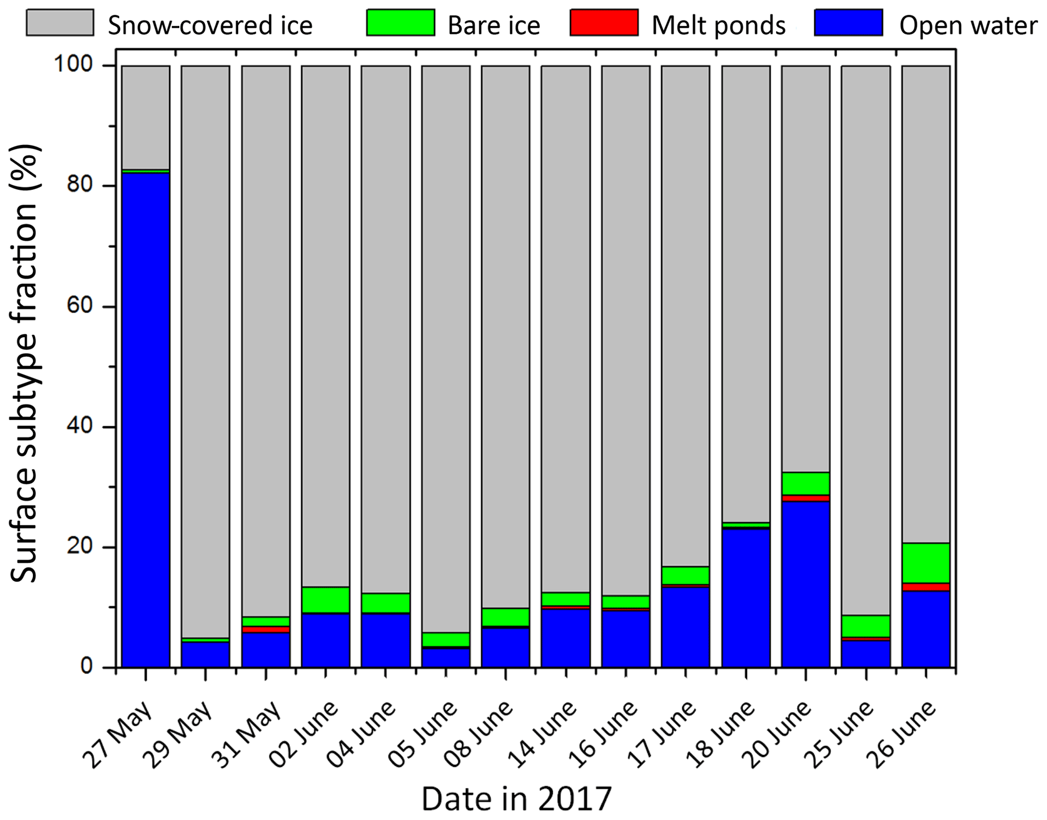
Figure 5Subtype fractions of ice and water surface for selected flight sections of Polar 6 during ACLOUD/PASCAL.

Download

3.1 Procedure

The validation of the SIS albedo scheme of HIRHAM–NAOSIM comprises two components: (a) the surface albedo itself (Sect. 3.2) and (b) the surface subtype fraction parameterization (Sect. 3.3). The procedure is illustrated in Fig. 6. The characterization of the surface is based on the digital camera images. For each time step of the images the derived surface albedo from the pyranometers and the surface temperature of the KT19 is selected.

Figure 6Flow chart of validation procedure of (a) surface albedo (blue background) and (b) surface type fraction (red background) parameterization.

Download

In step (a) the measured surface albedo was compared with the calculated albedo based on the surface subtype fractions deduced from the camera images. T_surf is taken to determine the temperature-dependent function f(T_surf) according to Eq. (4). Since Eq. (4) will be representative for one scene, only images with 90 % sea ice coverage were selected to omit temperature variations in the field of view of the pyranometer caused by different temperatures of open water and sea ice. Surface subtype fractions derived by the camera were calculated based on two approaches: (i) the summation of area sizes of similar surface types (linear approach) and (ii) similar to (i) but additionally with a weighting by the cosine of the viewing angle. The later approach takes into account that the irradiance is defined as the angular integration of the radiance weighted by the cosine of the viewing angle. This implies that the reflected radiation from side directions has a minor contribution relative to the radiation coming from the nadir direction. For a precise validation of Eq. (2) the albedo needs to be measured for all individual surface subtypes close to the surface. Aircraft observations always integrate over a larger area. Therefore, approach (i) might lead to uncertainties due to the neglect of cosine weighting. For this reason, the derived surface subtype fractions of both approaches are compared. Mean surface subtype fractions over the different flights were calculated and mean differences not larger than 2 % were found between the two approaches (i) and (ii). The correlation coefficient of the linear regressions between the surface subtype fractions of both approaches were larger than 0.98. Because of this approximate equality the comparison of measured and parameterized SIS albedo was simplified using only the derived surface subtype fractions, which were based on the linear approach.

Since the digital camera images deliver surface subtype fractions of snow-covered ice, melt ponds, bare ice, and open water, the individual subtype fractions have to be adapted for the application of Eq. (2). There, only the fractions of the sea ice subtypes are considered to weight α_s, α_m, and α_bi and to calculate the overall SIS albedo α_si. Therefore, the surface subtype fractions are rescaled with respect to their total sum.

In step (b) the fraction parameterization of snow-covered sea ice and melt ponds (Eqs. 5 and 6) is validated against estimated surface subtype fractions derived from the digital images. The surface subtype fraction parameterization is based on measured surface temperatures from the KT19 and snow depth data provided from the Magna probe. The selection of cases is limited compared to the SIS albedo scheme validation, caused by the availability of snow depth data in the surroundings of the aircraft flight paths. Only flight sections in the vicinity of the ice floe station were taken into account. Since snow depth is highly variable (Fig. 3), the parameterization was applied for the whole distribution of snow depth for the individual days and the measured KT19 temperature. Out of this, the mean parameterized surface subtype fraction for each image time step is compared to the measured fraction of sea ice subtypes. Only scenes with total ice coverage of 95 % were considered. Finally, the SIS albedo parameterization is applied based on the modeled surface subtype fractions from step (b).

3.2 Application of the sea ice albedo parameterization

Histograms of the measured and parameterized SIS albedo based on measured surface subtype fractions and surface temperature for individual days during ACLOUD/PASCAL are shown in Fig. 7. The days 27 May and 20 June were excluded here because the number of cases per day was fewer than 50. This minimum sample size (n) was approximated by

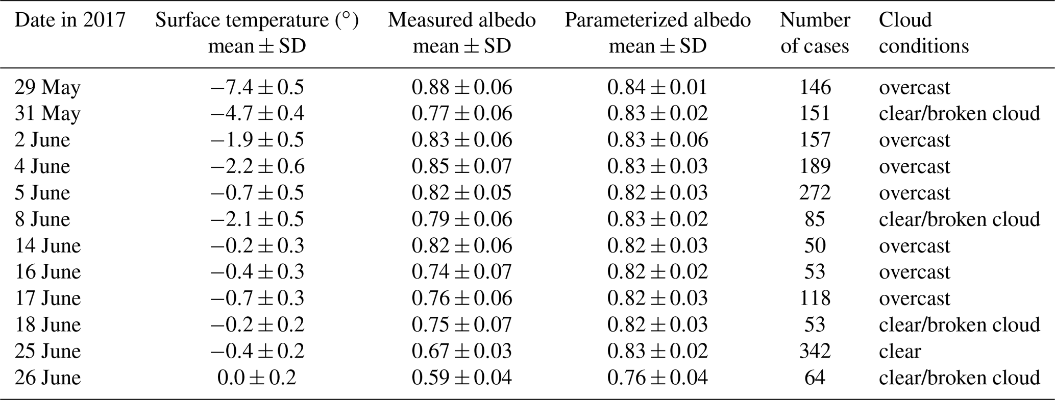
where z≈2 represents a confidence level of 95%, σ² is the variance, and e equals the assumed precision of the mean albedo (Mathews, 2010). Taking the measured variance (0.07²) and the desired albedo uncertainty (0.02) into account, n needs to be larger than 49. The distributions indicated by the thick colored lines in Fig. 7 represent the results for a sea ice cover larger than 90 %. Additionally, all cases independent of sea ice coverage are plotted by thin solid lines. Table 2 summarizes the daily mean measured and parameterized SIS albedo together with their standard deviation of the shown distributions.

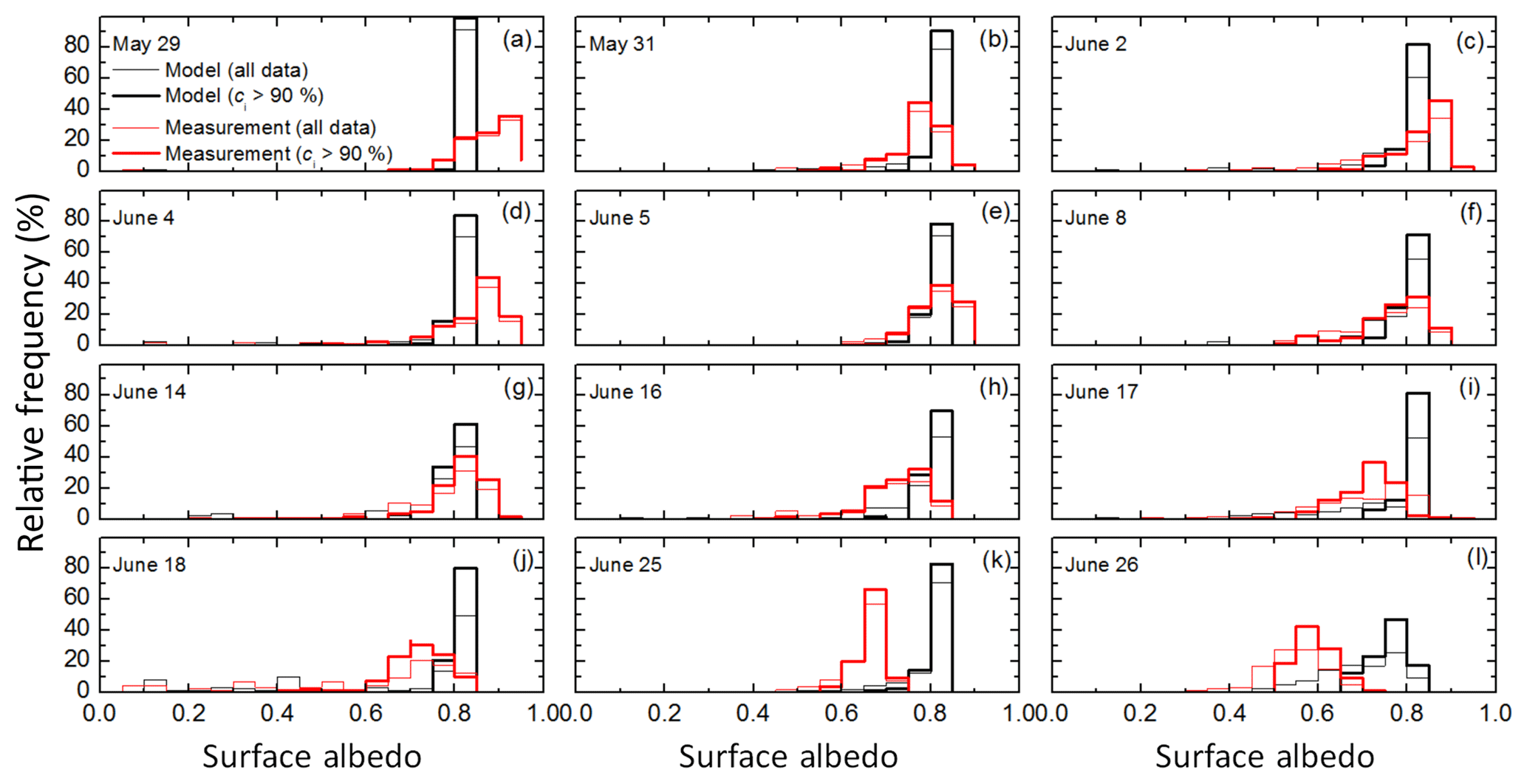
Figure 7(a)–(l) Histograms of measured (red) and parameterized (black) surface albedo for all selected days. Thick lines represent the cases when more than 90 % of the surface is covered by sea ice. Thinner lines show all cases matching the selection criteria described in Sect. 2.2.

Download

The impact of open water within the field of view becomes mainly obvious for 18 and 26 June, when measured and parameterized SIS albedo also exhibit modes for smaller albedo values. For 18 June, the cases showing open water are dominated by subtype fractions c_ow>50 %, which results in α<0.5. In contrast, on 26 June, the images indicate the presence of ice floes with c_ow lying in the range between 20 % and 30 %, leading to α>0.5.

Two issues become noticeable when comparing the histograms. First, the parameterized SIS albedo shows a narrower distribution than the measured surface albedo. This is especially pronounced for scenes of uniform surface type and surface temperatures, which result in f(T_surf)=0 according to Eq. (4). In particular, on 29 May temperatures below −4 ^∘C over mostly snow-covered ice were measured. This results in a narrow distribution of the SIS albedo, which corresponds to the maximum albedo of snow-covered ice α_max=0.84 (Table 1). Only with an increase in temperature, when snow melting is considered in the SIS albedo parameterization and when multiple sea ice subtypes are identified in the image, is a broader distribution of parameterized albedo observed (26 June, Fig. 7l).

The second issue obvious from Fig. 7 is the temporal change when comparing both SIS albedo distributions. In the beginning of the campaign, when T_surf is lower than −2 ^∘C, the parameterized SIS albedo is systematically lower than the measured one (see also Table 2). In contrast, at the end of June this relation is reversed, while in the transition period the mean parameterized SIS albedo agrees well with the measurements, particularly for overcast cloud conditions. An exception to this trend was found for 31 May when the mean measured albedo of sea ice (α=0.77) was lower than the parameterized albedo (α=0.83). Sea ice concentration maps from the AMSR sensor show that the ice edge moves further north from 29 to 31 May, in the area of the flight tracks. This results in an increase in surface roughness on 31 May, which is also apparent from the digital camera images. Furthermore, different illumination conditions were observed on both days. While on 29 May the SIS albedo was measured under overcast conditions, broken clouds all the way to clear sky occurred on 31 May. The effect of cloud conditions on the surface albedo was already discussed by several authors before, such as Choudhury and Chang (1981) and Yamanouchi (1983) or more recently Pirazzini et al. (2015). Clouds affect the spectral behavior of the incident solar radiation and the directional dependence. In cloudy conditions the incoming radiation field is dominated by the diffuse component, whereas the transmission of radiation through the clouds is wavelength-dependent. Since the solar radiation is mainly absorbed by cloud particles in the near-infrared spectral range, a larger fraction of visible to global radiation is incident on the surface compared to clear-sky conditions. Furthermore, the enhanced multiple scattering between clouds and snow surface additionally contributes to the spectral shift of the incident radiation. Consequently, the broadband albedo increases under cloudy conditions.

Effects of the solar zenith angle (SZA) on the observed differences in Fig. 7a, b can be excluded here since for both days the SZA was in the range between 65 and 68^∘. Thus, the likely dominating effect of the clear-sky conditions together with the increased roughness lead to a decrease in the measured SIS albedo, whereas the snow metamorphism causing larger grain sizes is probably of minor importance since the surface temperature is below melting temperature ($T_{\mathrm{surf}}=-\mathrm{4}$ ^∘C).

Table 2Averaged SIS surface albedo and standard deviation (SD) of each flight retrieved from aircraft observation and parameterization. Additionally, the mean temperature, number of cases, and the illumination conditions are given. Note that only cases with an ice fraction larger than 90 % are considered here.

Download Print Version | Download XLSX

In the HIRHAM–NAOSIM albedo scheme, the parameterized SIS albedo of all surface subtypes only depends on the temperature and the predefined maximum and minimum thresholds of the surface albedo (Eq. 3). This relation is tested against the measured temperature dependence. For the selected flights, the fraction of melt ponds and bare ice subtypes have never exceeded the 90 % threshold, which was set to assume a homogeneous surface type. Therefore, the evaluation of the relationship between temperature and SIS albedo based on the ACLOUD data set is limited to the snow-covered sea ice subtype. All data were filtered with respect to a fraction of c_s = 100 %. The mean values of surface temperature and SIS albedo for all selected flights are shown in Fig. 8a. The data set is separated according to the daily illumination conditions, either overcast (closed symbols) or clear sky/broken cloud (open symbols). Additionally, the corresponding parameterized SIS albedo is marked by the dashed line, revealing the sharp drop of albedo around 0 ^∘C.

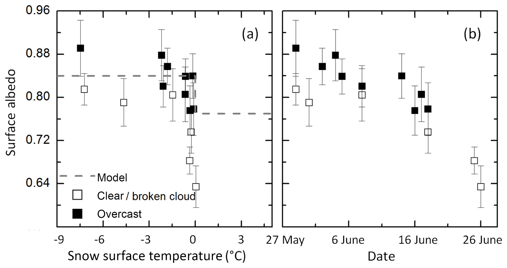
Figure 8Mean albedo of snow-covered ice scenes as a function of surface temperature (a) and time (b) separated into clear sky/broken clouds and overcast situations. Vertical bars indicate the standard deviation of the averaged surface temperature on each day. The symbols represent the measured albedo and the dashed gray line represents the parameterized albedo.

Download

Figure 8 illustrates that the measured SIS albedo does not follow the surface temperature dependence as assumed by the parameterization. In general, the albedo decreases over the early summer with changing temperature. A short-term temperature increase does not necessarily result in a sharp drop of surface albedo as would be predicted by Eq. (3). In fact, the decrease in SIS albedo is mainly caused by a temporal change (Fig. 8b) in the surface properties, as grain size and snow thickness. As obvious from Eq. (3), both parameters are not considered in the SIS albedo parameterization of HIRHAM–NAOSIM. The temporal decrease in albedo was already observed in Fig. 4b with the difference that Fig. 4b also includes selected scenes of multiple subtypes. Consequently, the conversion of surface subtypes results in not only the decrease in SIS albedo, but also the temporal change in snow reflection properties of the snow-covered sea ice subtype, which accounts for the largest fraction of all subtypes in the studied cases (see Fig. 5).

In addition to snow property changes, the illumination conditions might also have an impact on the variation in the surface albedo (Choudhury and Chang, 1981; Pirazzini et al., 2015). Lower SIS albedo values were measured for all cases under cloudless and broken cloud conditions compared to overcast situations with similar surface temperatures ranges. From Fig. 8 it is evident that the illumination effect is of the same importance as the snow type variation (e.g., change in roughness, grain size, density) within the observed temperature range. This indicates that the SIS albedo parameterization should also take account of the dependence on cloud cover fraction.

3.3 Application of the surface type classification and full albedo scheme

In this section, the fraction parameterization following Eqs. (5) and (6) is applied including measured snow depth and surface temperature data. While surface temperature data were collocated in time and space with the digital camera observations, the ground-based measured snow depth data were not sampled directly below the aircraft on the selected flight days. Therefore, the data set was further limited to cases where the aircraft position is not more than 50 km from the points of snow depth measurements. In addition, the flight date may differ by 1 d from the ground-based observation of snow depth. Restrictions in both space and time should ensure the representativeness of local point measurements of the snow depth for the selected area.

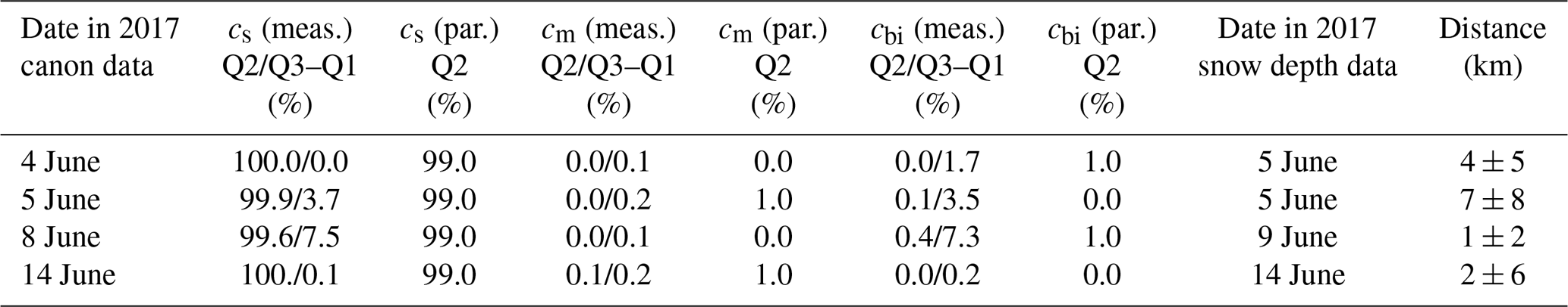
Table 3 summarizes the statistics of the measured and parameterized fractions for each day. Here, the median instead of the daily mean is calculated to exclude the effect of outliers. Furthermore, the distance of the upper and the lower quartiles is given to estimate the range of measured fractions. According to Eq. (5), the snow depth determines the fraction of snow-covered ice. The maximum value of c_s of 0.99 is reached for a snow depth larger than 10 cm as defined in Eq. (5). The snow depth distributions in Fig. 3 reveal that for all days, apart from 15 June, the majority of snow depth values are larger than 10 cm. Therefore, it is not surprising that the parameterized fractions of snow-covered ice are 99 % in all these cases independent of the shape of the snow depth distribution. The remaining 1 % fraction is related to either melt ponds or bare ice, as defined by the surface temperature. Equation (6) determines the melt pond fractions and indirectly the fraction of the bare ice subtype because the sum of all three subtypes adds up to one. From the temperatures measured along the selected flight paths, melt ponds were calculated for the days 5 and 14 June. In summary, the measured and parameterized surface subtype fractions are in very good agreement. However, the variation in surface types is quite low since the observed region around the ice floe is covered almost completely by snow. Only in the second half of June, where now snow depth data were measured, the surface type distribution got more complex.

Table 3Measured (meas.) and parameterized (par.) subtype fractions of snow-covered ice (c_s), melt ponds (c_m), and bare ice (c_bi) for selected flight sections on individual days. Q2 stands for the median; Q3–Q1 represent the distance of the upper and lower quartiles. Additionally, the horizontal distance between Polar aircraft and the Magna probe is given.

Download Print Version | Download XLSX

Finally, the calculated fractions as derived above were used as input for Eq. (2) to compute the SIS albedo α_i for all sections connected to the ground-based snow depth measurements on the ice floe. Then, together with measured open water fractions, the final SIS albedo α was derived according to Eq. (1). In Fig. 9 the daily averaged albedo values are presented as a box-and-whisker plot. As for the subtype fraction statistics, the median and the quartiles are shown, since the number of cases is quite low (fewer than 10 for 8 and 14 June) compared to the studied scenes shown in Sect. 3.3 (minimum 50 cases). No variation in the parameterized SIS albedo is found on most of the days, due to the constant relation between the subtype fractions. The variation visible on 5 and 8 June arises from the variable fraction of open water with a subtype albedo of α_ow=0.1. However, the variability of the measured SIS albedo cannot be fully reproduced by the albedo scheme. The absolute values of measured and parameterized SIS albedo exhibit the largest differences for cases which were measured under cloudless/broken cloud conditions (8 June). As the surface temperature dependence function is the main parameter, the resulting modeled SIS albedo for T_surf>0 ^∘C corresponds with α_s=α_min, while on the other days with T_surf<0 ^∘C, α_s equals α_max.

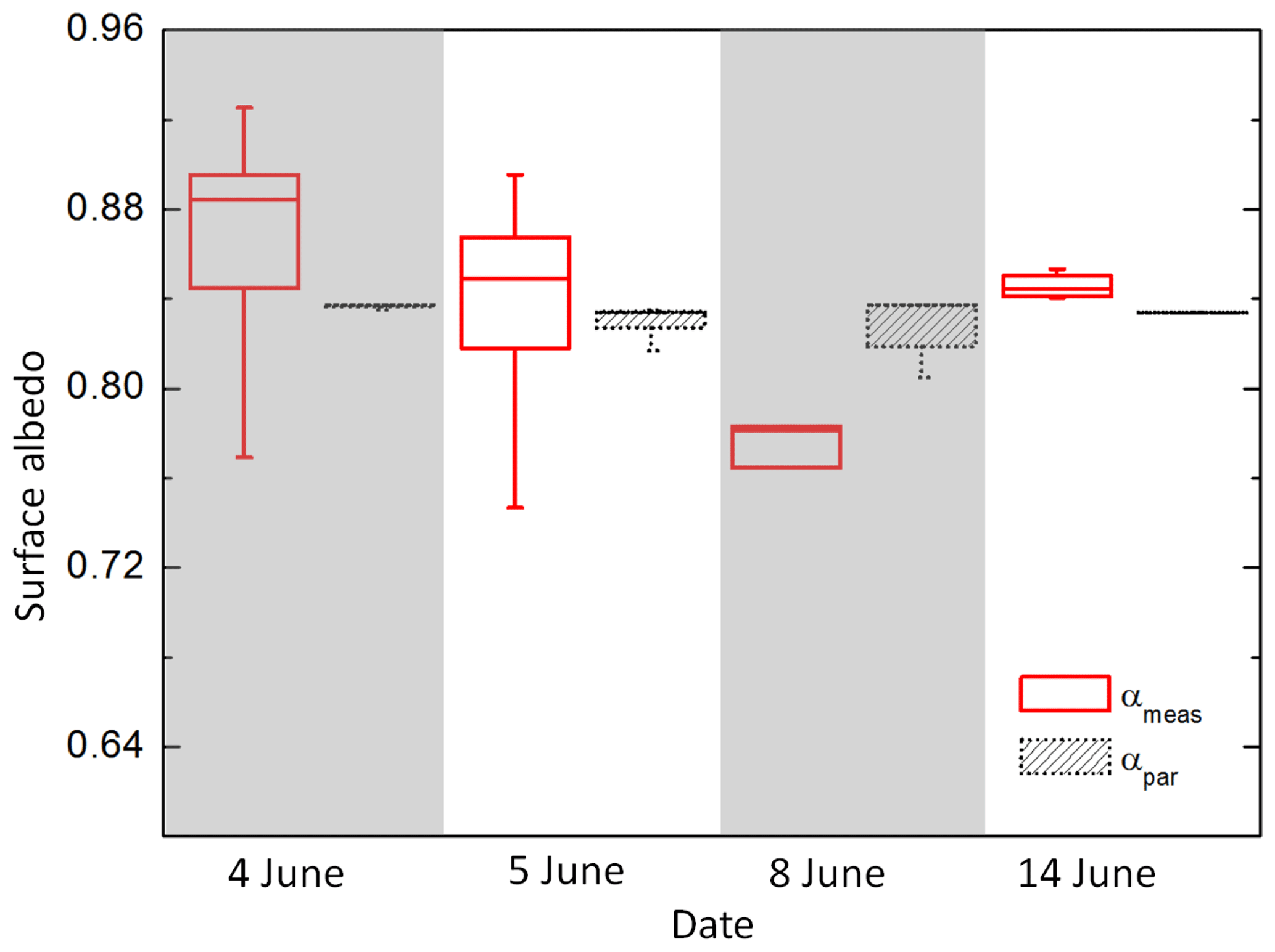
Figure 9Box-and-whisker plot of measured (red solid lines) and parameterized (black dotted lines) surface albedo for selected flight paths in the surrounding of the ice floe where snow depth data were sampled. Minimum and maximum values are displayed as vertical bars. The boxes indicate the 25th, 50th (median), and 75th percentiles of the distribution. The individual days are separated by alternate gray and white areas.

Download

3.4 Adjustment of the sea ice albedo parameterization

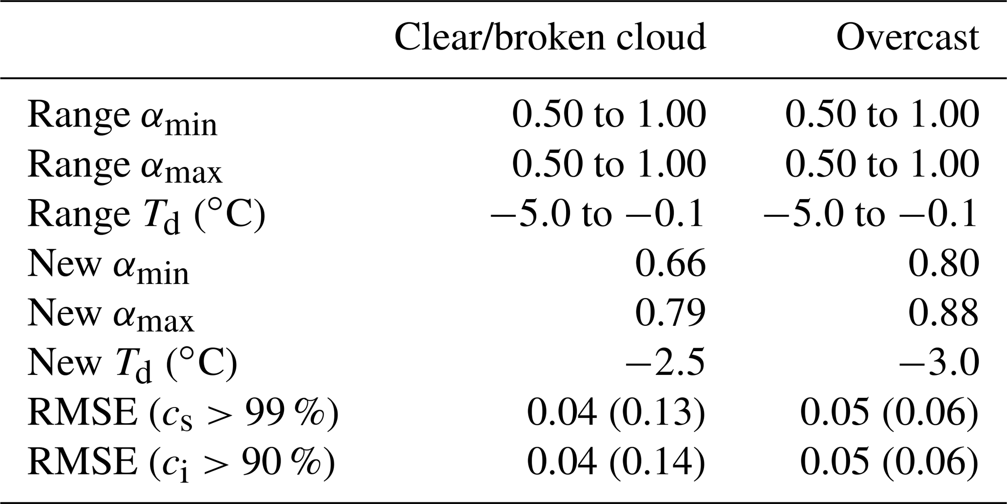
From the 12 flight days during the ACLOUD campaign, differences between modeled and measured SIS albedo (α_par, α_meas) were attributed to the impact of illumination conditions (cloudiness) and the choice of minimum and maximum surface albedo values used in Eq. (3). Since uniform subtypes were limited to measurements over snow-covered ice, an adjustment of the parameters α_max and α_min and the temperature threshold T_d is only provided for this subtype. All data points with c_s>99 % were separated into two classes depending on the cloud cover, similar to the classification shown in Fig. 8. The three parameters were varied systematically to find the optimum combination with a minimum RMSE as calculated by

The final parameters and the corresponding RMSE values for overcast and clear/broken cloud conditions are summarized in Table 4 together with the variation range of α_max, α_min, and T_d. The minimum and maximum albedo values were tested in a range of 0.5 up to 1.0 in steps of 0.01. The adjusted albedo parameters clearly describe the two cloud conditions with higher minimum and maximum values (0.80, 0.88) for overcast conditions and lower values (0.66, 0.79) for clear-sky and broken cloud situations compared to the suggested numbers given in the original sea ice albedo scheme from Dorn et al. (2009) with α_min=0.77 and α_max=0.84 (Table 1). Also, the threshold temperature was adjusted from −0.01 to −2.5 ^∘C (cloudless/broken cloud) and −3.0 ^∘C (overcast). The greatest improvement was found for the parameterization of clear-sky surface albedo, where the RMSE values for all cases with c_s>99 % reduced from 0.13 to 0.04, and for all data matching c_i>90 % from 0.14 to 0.04. For overcast situations, the RMSE reduces only slightly from 0.06 to 0.05 for c_s>99 % and for cases with c_i>90 %.

Table 4Variation range of minimum and maximum albedo values for snow-covered ice and threshold temperature for the adjustment of the sea ice albedo parameterization following Eqs. (3) and (4). The albedo and temperature are modified in steps of 0.01 and 0.1^∘C, respectively. Final fitting values of α_min, α_max, and T_d are given for clear/broken cloud and overcast conditions together with the new and old (in brackets) RMSE values.

Download Print Version | Download XLSX