the Creative Commons Attribution 4.0 License.
the Creative Commons Attribution 4.0 License.
 | 08 Jul 2019
Antarctic ice shelf thickness change from multimission lidar mapping
Tyler C. Sutterley
Thorsten Markus
Thomas A. Neumann
Michiel van den Broeke
J. Melchior van Wessem
Stefan R. M. Ligtenberg
We calculate rates of ice thickness change and bottom melt for ice shelves in West Antarctica and the Antarctic Peninsula from a combination of elevation measurements from NASA–CECS Antarctic ice mapping campaigns and NASA Operation IceBridge corrected for oceanic processes from measurements and models, surface velocity measurements from synthetic aperture radar, and high-resolution outputs from regional climate models. The ice thickness change rates are calculated in a Lagrangian reference frame to reduce the effects from advection of sharp vertical features, such as cracks and crevasses, that can saturate Eulerian-derived estimates. We use our method over different ice shelves in Antarctica, which vary in terms of size, repeat coverage from airborne altimetry, and dominant processes governing their recent changes. We find that the Larsen-C Ice Shelf is close to steady state over our observation period with spatial variations in ice thickness largely due to the flux divergence of the shelf. Firn and surface processes are responsible for some short-term variability in ice thickness of the Larsen-C Ice Shelf over the time period. The Wilkins Ice Shelf is sensitive to short-timescale coastal and upper-ocean processes, and basal melt is the dominant contributor to the ice thickness change over the period. At the Pine Island Ice Shelf in the critical region near the grounding zone, we find that ice shelf thickness change rates exceed 40 m yr−1, with the change dominated by strong submarine melting. Regions near the grounding zones of the Dotson and Crosson ice shelves are decreasing in thickness at rates greater than 40 m yr−1, also due to intense basal melt. NASA–CECS Antarctic ice mapping and NASA Operation IceBridge campaigns provide validation datasets for floating ice shelves at moderately high resolution when coregistered using Lagrangian methods.


Most of the drainage from the Antarctic ice sheet is through its peripheral ice shelves, floating extensions of the land ice that cover 75 % of the Antarctic coastline and represent 10 % of the total ice-covered area (Cuffey and Paterson, 2010; Rignot et al., 2013). The modern-day thinning of Antarctic ice shelves may make the shelves more susceptible to fracture and overall collapse (Shepherd et al., 2003; Fricker and Padman, 2012). The mass budget of an ice shelf is the sum of several mass gain and loss terms (Thomas, 1979). Mass is gained by the advection of ice from the land, the accumulation of snow at the surface, and the freezing of seawater at the ice shelf base (Thomas, 1979). Mass is lost by the runoff of surface meltwater, the erosion and sublimation of snow by wind, the sublimation of snow at the surface of the shelf, the melting of ice at the base of the shelf, and the calving of icebergs (Thomas, 1979).
Floating ice shelves can exert control on the grounded ice sheet's overall stability by buttressing the flow of the glaciers upstream (Dupont and Alley, 2005). The response of inland glaciers to ice shelf variations is complicated and is dependent on both the inland bed topography and the ice shelf geometry (Goldberg et al., 2009; Gagliardini et al., 2010; Gudmundsson, 2013). Presently, several ice shelves across Antarctica are losing mass, which may have led to the acceleration and intensified discharge of inland ice (Pritchard et al., 2012; Depoorter et al., 2013; Paolo et al., 2016). In 2003, a year after the collapse of the Larsen-B Ice Shelf, some tributary glaciers draining into the Weddell Sea from the Antarctic Peninsula flowed at rates 2–8 times their 1996 flow rates (Rignot et al., 2004). These glaciers continued flowing at the accelerated rates several years after the collapse (Rignot et al., 2008; Berthier et al., 2012). Glaciers of the Amundsen Sea Embayment (ASE) in West Antarctica have experienced significant increases in surface velocity, dynamic thinning, and grounding line retreat since the 1990s (Rignot et al., 2002, 2014; Pritchard et al., 2009; Flament and Rémy, 2012). The dynamical change of these glaciers likely stems from increases in subshelf circulation and heat content of warm Circumpolar Deep Water, which enhanced ocean-driven melt causing thinning of the buttressing peripheral ice shelves (Jacobs et al., 2011).
Here, we compile ice shelf thickness change rates calculated using a suite of airborne altimetry datasets, which have been consistently processed and coregistered. We provide a set of coregistered laser altimetry datasets for evaluating estimates from satellite altimetry, photogrammetry, and model outputs. The main objectives of this study are to (i) calculate ice shelf thickness change rates, (ii) investigate processes driving the changes in the shelf, (iii) investigate the sensitivity of spatial and temporal sampling to overall estimates, and (iv) evaluate different methods of calculating elevation change rates over ice shelves. In the following sections, we discuss the coregistration method, the geophysical corrections applied, the results for a sample set of ice shelves, and the overall implications of the results for ice shelf studies.
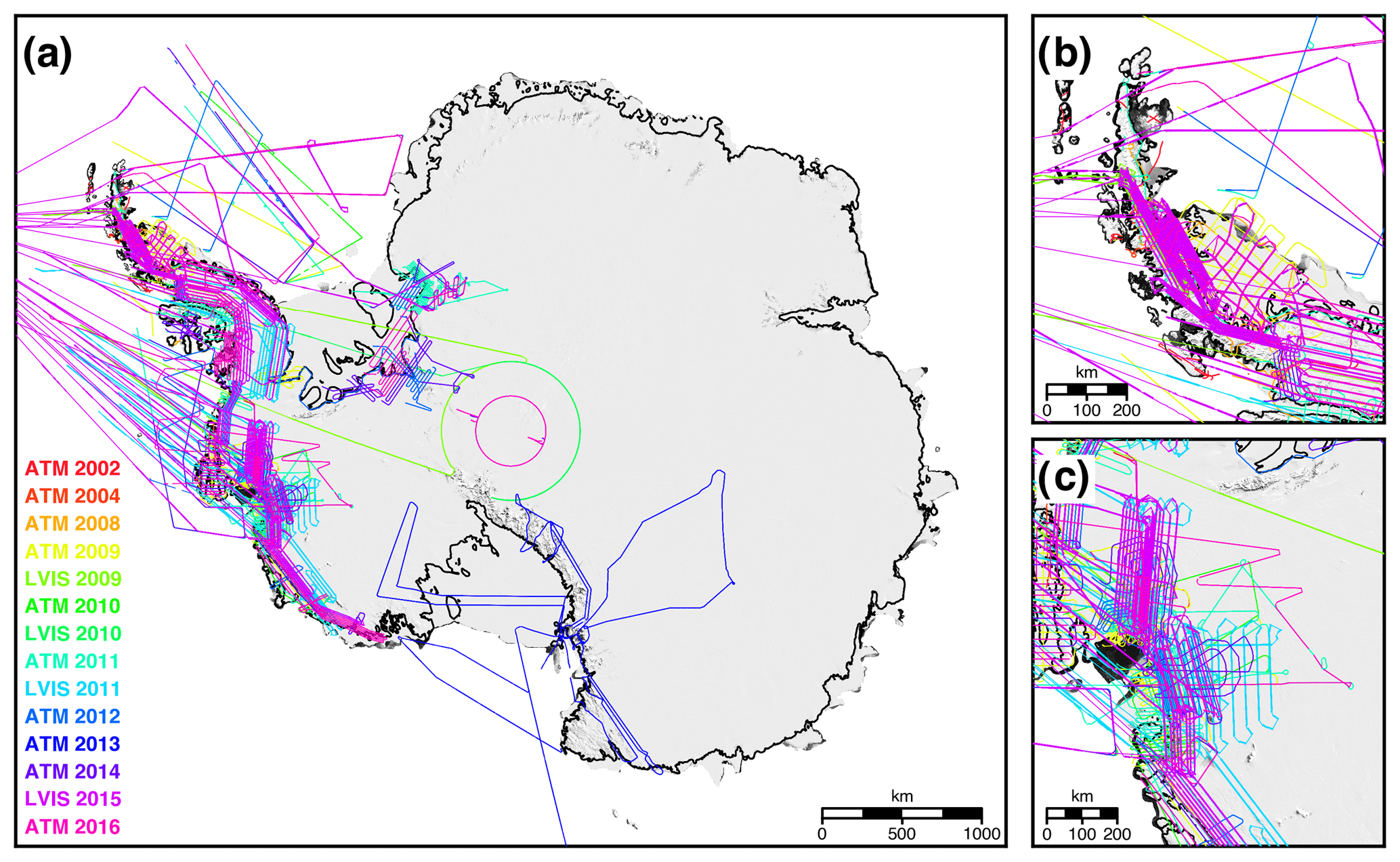
Figure 1NASA–CECS Pre-IceBridge and NASA Operation IceBridge campaign flight lines over (a) Antarctica, (b) the Antarctic Peninsula, and (c) the Amundsen Sea Embayment from 2002 to 2016 colored by year of acquisition and laser ranging instrument. Antarctic grounded ice delineation provided by Mouginot et al. (2017b). Flight lines overlaid on a 2008–2009 MODIS mosaic of Antarctica (Haran et al., 2014).
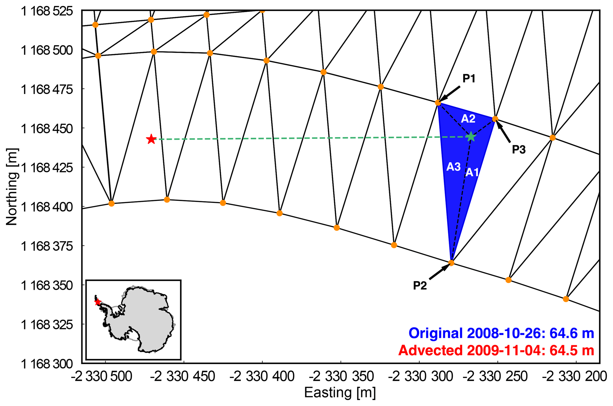
Figure 2Triangulated mesh formulated around an advected 2008 ATM (Airborne Topographic Mapper) flight line point using points from a 2009 ATM flight line (orange dots). The red star denotes the location of the original point, the green star denotes the parcel location after advection, and the dashed green line is the path of advection. P1, P2, and P3 represent the three vertices of the triangle housing the advected ATM point. Elevation values at each vertex point are weighted in the interpolation by their respective areas, A1, A2, and A3. The inset map shows the location of the main figure.
Our airborne lidar measurements are Level-2 Airborne Topographic Mapper (ATM) Icessn and Land, Vegetation and Ice Sensor (LVIS) datasets provided by the National Snow and Ice Data Center (NSIDC) (Thomas and Studinger, 2010; Studinger, 2014; Blair and Hofton, 2010). ATM is a conically scanning lidar developed at the NASA Wallops Flight Facility (Thomas and Studinger, 2010). ATM instruments have flown in Antarctica since 2002 as part of both the NASA–Centro de Estudios Científicos (CECS) Antarctic ice mapping and NASA Operation IceBridge campaigns. The Level-2 ATM Icessn data are calculated by fitting planar surfaces to the original ATM point clouds at approximately 40 m spacing along track (Studinger, 2014). LVIS is a large-swath scanning lidar which flew in Antarctica in 2009, 2010, 2011, and 2015 and was developed at the NASA Goddard Space Flight Center (Blair et al., 1999; Hofton et al., 2008). For the data release available for Antarctica (LDSv1), the Level-2 LVIS data provide three different elevation surfaces computed from the Level-1B waveforms: the highest and lowest returning surfaces from Gaussian decomposition, and the centroidal surface (Blair and Hofton, 2010). Here, we use the lowest returning surface when the waveform resembles a single-peak gaussian and the centroid surface when the waveform is multipeaked. The spatial coverages of each instrument in Antarctica for the campaigns prior to and during NASA Operation IceBridge are shown in Fig. 1. The elevation datasets from each instrument are converted to the 2014 solution of the International Terrestrial Reference Frame (ITRF) (Altamimi et al., 2016). In order to track changes in ice shelf freeboard, the ellipsoid heights for each instrument were converted to be in reference to the GGM05 geoid using gravity model coefficients provided by the Center for Space Research (Ries et al., 2016). Changes in ice shelf freeboard are converted into changes in ice thickness by assuming hydrostatic equilibrium following Fricker et al. (2001). Uncertainties for each instrument were calculated following Sutterley et al. (2018).
2.1 Integrated analysis of altimetry
We calculate rates of elevation change by comparing a set of measured elevation values with a set of interpolated elevation values from a different time period after allowing for the advection of the ice (Sutterley et al., 2018; Moholdt et al., 2014; Shean et al., 2018). Each point in a flight line is advected from its original location by integrating the Rignot et al. (2017) MEaSUREs (Making Earth System Data Records for Use in Research Environments) static velocity data derived from synthetic aperture radar (SAR) using a fourth-order Runge–Kutta algorithm. For each data point in a flight line, a set of Delaunay triangles is constructed from a separate flight line using all data points within 300 m from the final location of the advected point (Pritchard et al., 2009, 2012; Rignot et al., 2013). If the advected point lies within the confines of the Delaunay triangulation convex hull, the triangular facet housing the advected point is determined using a winding number algorithm (Sutterley et al., 2018). The new elevation value is calculated using barycentric interpolation with the elevation measurements at the three triangle vertices (Fig. 2). The elevation at each vertex point is weighted in the interpolation by the area of the triangle created by the enclosed point and the two opposing vertices (Sutterley et al., 2018).
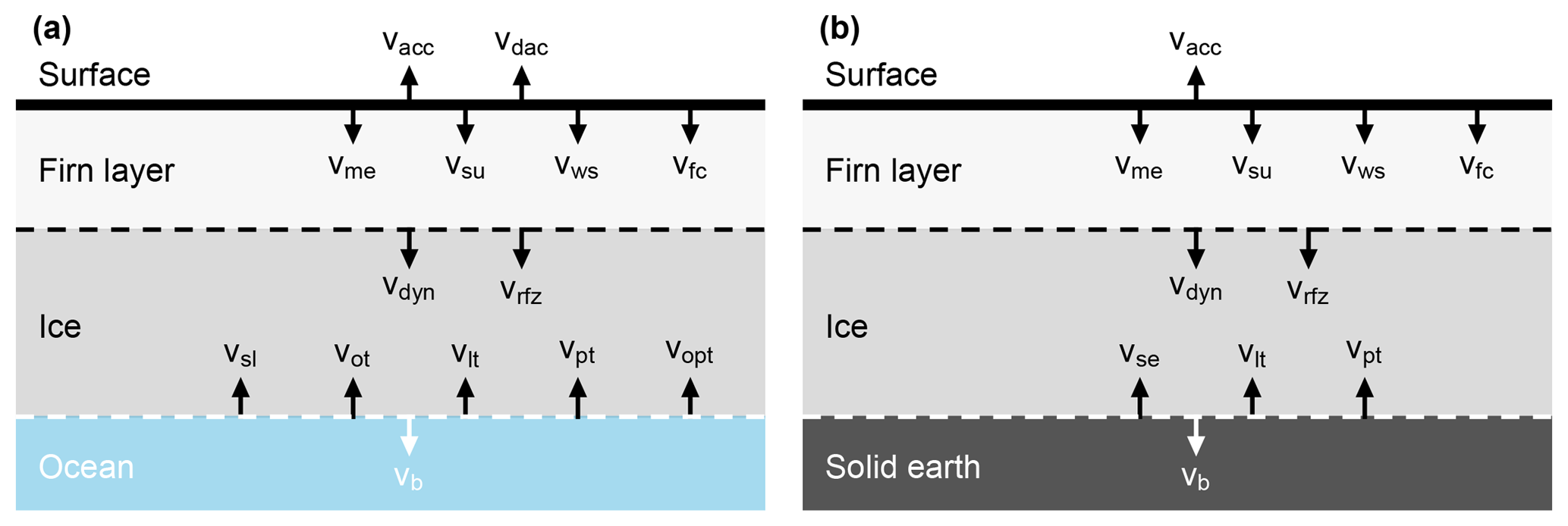
Figure 3Representation of processes contributing to surface elevation changes for (a) ice shelves and (b) grounded ice. Modified from Ligtenberg et al. (2011) and Zwally and Li (2002). Processes represented in schematic: accumulation (vacc), dynamic atmosphere (vdac), snowmelt (vme), sublimation (vsu), wind scour (vws), firn compaction (vfc), ice dynamics (vdyn), meltwater refreeze and retainment (vrfz), solid Earth uplift (vse), sea level (vsl), ocean tides (vot), load tides (vlt), load pole tides (vpt), ocean pole tides (vopt), and basal melt (vb).
Assuming that the ice shelf surfaces are not curved over the scale of the individual triangular facet (∼10–100 m), interpolating to the advected coordinates will compensate for minor slopes in the ice shelf surface so that the elevations of equivalent parcels of ice can be compared in time (Pritchard et al., 2009). At this scale (below 100–200 m), the topographic relief of uncrevassed ice is primarily due to slopes in the ice surface and a planar assumption should be largely valid (Markus et al., 2017). Rough terrain, snow drifts, and low-lying clouds will contaminate the lidar elevation values for the interpolation. In order to limit the effect of contaminated points, the elevation measurements are filtered using the robust dispersion estimator (RDE) algorithm described in Smith et al. (2017). In order to minimize the possibility of coregistering measurements over ice shelves with measurements over grounded ice near the grounding zone or measurements over the ocean, sea ice floes, and icebergs, we only include points that are on the ice shelf for the compared time periods using grounded ice delineations from Rignot et al. (2016) and Mouginot et al. (2017b) and ice shelf extent delineations manually digitized from Landsat imagery courtesy of the U.S. Geological Survey and MODIS imagery from Scambos et al. (2001).
For comparison, we compile elevation change measurements using an Eulerian approach with the triangulated-irregular-network (TIN) technique outlined in Sutterley et al. (2018) and a Lagrangian overlapping footprint approach following Slobbe et al. (2008) and Moholdt et al. (2014). The Eulerian TIN scheme follows the methods of Pritchard et al. (2012) and Rignot et al. (2013) that used data from the NASA ICESat mission. Measurements compiled using the Eulerian TIN scheme have been made comparable to the Lagrangian thinning rates by adding the effects of strain using the relation from Moholdt et al. (2014).
where ρw and ρice are the densities of sea water and meteoric ice, respectively, and (V⋅∇M) is the ice shelf thickness gradient advection. For calculating the mass divergence for comparing Eulerian- and Lagrangian-derived ice thickness change rates, we use ice thickness data and uncertainties from Bedmap2, which are primarily derived from Griggs and Bamber (2011) for ice shelves (Fretwell et al., 2013). The ice thickness data from Griggs and Bamber (2011) are calculated assuming hydrostatic equilibrium, which should be valid for most areas downstream of the 1–8 km wide grounding zones (Brunt et al., 2010, 2011). The Lagrangian overlapping footprint approach uses the same fourth-order Runge–Kutta algorithm to advect the coordinates of the original elevation measurement to a predicted parcel location at a separate time. If any measurements from the separate flight line lie within 100 m of the advected point, the elevation measurement closest in Euclidean distance to the advected point is compared against the original measurement.

Figure 4Surface elevation change of the Larsen-B remnant and Larsen-C Ice Shelf derived using (a) Eulerian TINs corrected for strain, (b) Lagrangian TINs, and (c) Lagrangian overlapping footprint schemes for the period 2009–2016. The rms differences in elevation change from a measurement point for all points within 1 km for the (d) Eulerian TINs corrected for strain, (e) Lagrangian TINs, and (f) Lagrangian overlapping footprint methods. The elevation change rates shown here are not RDE filtered (Smith et al., 2017). Antarctic grounded ice boundaries are provided by Mouginot et al. (2017b). Plots are overlaid on a 2008–2009 MODIS mosaic of Antarctica (Haran et al., 2014). The inset map denotes the location of the maps.
2.2 Geophysical corrections
We correct the elevation measurements for geophysical processes following most of the procedures that will be used with the initial release of ICESat-2 data (Markus et al., 2017; Neumann et al., 2018). The processes are described in the following sections and represented as a schematic in Fig. 3.
2.2.1 Tidal and nontidal ocean variation
Surface elevation changes due to variations in ocean and load tides are calculated using outputs from the Circum-Antarctic Tidal Simulation (CATS2008) model (Padman et al., 2008), a high-resolution inverse model updated from Padman et al. (2002). Surface heights were predicted for the M2, S2, N2, K2, K1, O1, P1, Q1, Mf, and Mm harmonic constituents and then inferred for 16 minor constituents following the PERTH3 algorithm developed by Richard Ray at the NASA Goddard Space Flight Center (Ray, 1999). Uncertainties in tidal oscillations were estimated using constituent uncertainties from King et al. (2011). We correct for changes in load and ocean pole tides due to changes in the Earth's rotation vector following Desai (2002) and IERS conventions (Petit and Luzum, 2010).
We correct for changes in sea surface height due to changes in atmospheric pressure and wind stress using a dynamic atmosphere correction (DAC) provided by https://www.aviso.altimetry.fr/en/data/products/auxiliary-products/atmospheric-corrections.html (AVISO, last access: 30 March 2018). The 6 h DAC product combines outputs of the MOD2D-g ocean model, a 2-D ocean model forced by pressure and wind fields from ECMWF based on Lynch and Gray (1979), with an inverse barometer (IB) response (Carrère and Lyard, 2003). Regional sea levels fluctuate due to changes in ocean dynamics, ocean mass, and ocean heat content (Church et al., 2011; Armitage et al., 2018). Nontidal sea surface anomalies are removed from the ice shelf data using multimission altimetry products computed by AVISO (https://www.aviso.altimetry.fr/en/data/products/sea-surface-height-products/global/msla-h.html, last access: 7 July 2017) and provided by Copernicus (Le Traon et al., 1998). The nontidal sea surface anomalies are added to estimates of mean dynamic topography, which is the mean deviation of the sea surface from the Earth's geoid due to ocean circulation. The sea surface anomalies are extrapolated from the valid ice-free ocean values to the ice shelf points following Paolo et al. (2016).
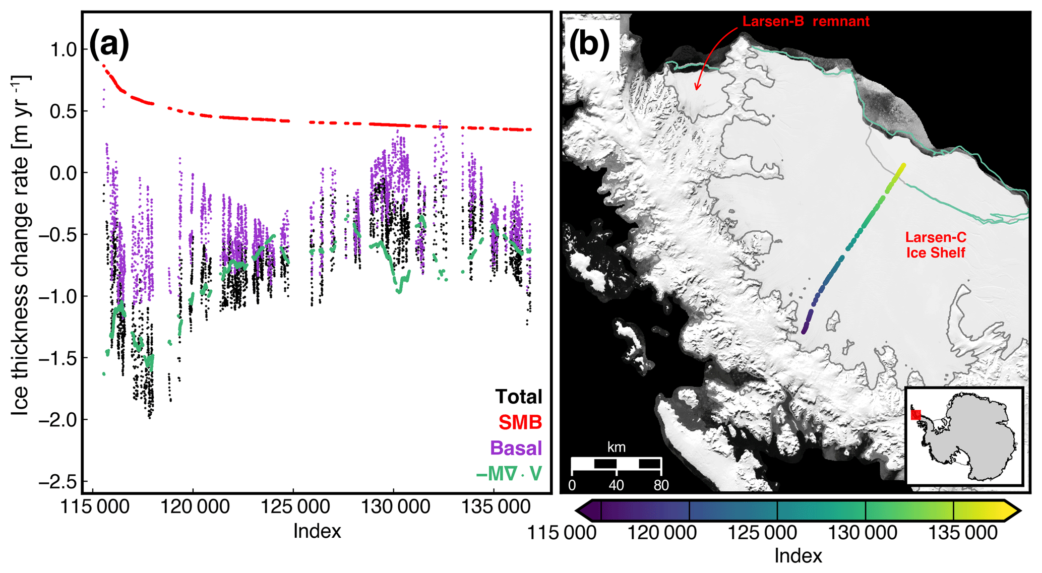
Figure 5Measured and estimated ice thickness change rates from 2008 to 2016 for a flight line over the Larsen-C Ice Shelf (a) starting near the Whirlwind Inlet with the total measured ice thickness change rate denoted in black, SMB from RACMO2.3p2 (XPEN055) denoted in red (van Wessem et al., 2016), the flux divergence terms combining ice velocities from MEaSUREs (Rignot et al., 2017) and ice thicknesses denoted in green, and the residual basal thickness change rates denoted in purple. The index denotes the ATM Icessn record number for 10 October 2008. Locations of coregistered records from the flight line are shown in (b). MEaSUREs interferometric synthetic aperture radar (InSAR)-derived Antarctic grounded ice boundaries are denoted in gray (Mouginot et al., 2017b). The 2016 and 2017 ice shelf extents delineated from MODIS imagery are denoted in green and light gray, respectively (Scambos et al., 2001). The map is overlaid on a 2008–2009 MODIS mosaic of Antarctica (Haran et al., 2014). The inset map denotes the location of the map.

Figure 6Ice thickness change (a–b) and estimated basal melt rates (c–d) of the Larsen-B remnant and Larsen-C Ice Shelf for two periods, 2002–2008 and 2008–2016. AI, CI, MI, WI, and MOI denote the Adie, Cabinet, Mill, Whirlwind, and Mobiloil inlets, respectively. MEaSUREs InSAR-derived Antarctic grounded ice boundaries are denoted in gray (Mouginot et al., 2017b). The 2016 and 2017 ice shelf extents delineated from MODIS imagery are denoted in green and light gray, respectively (Scambos et al., 2001). Plots are overlaid on a 2008–2009 MODIS mosaic of Antarctica (Haran et al., 2014). The inset map denotes the location of the maps.
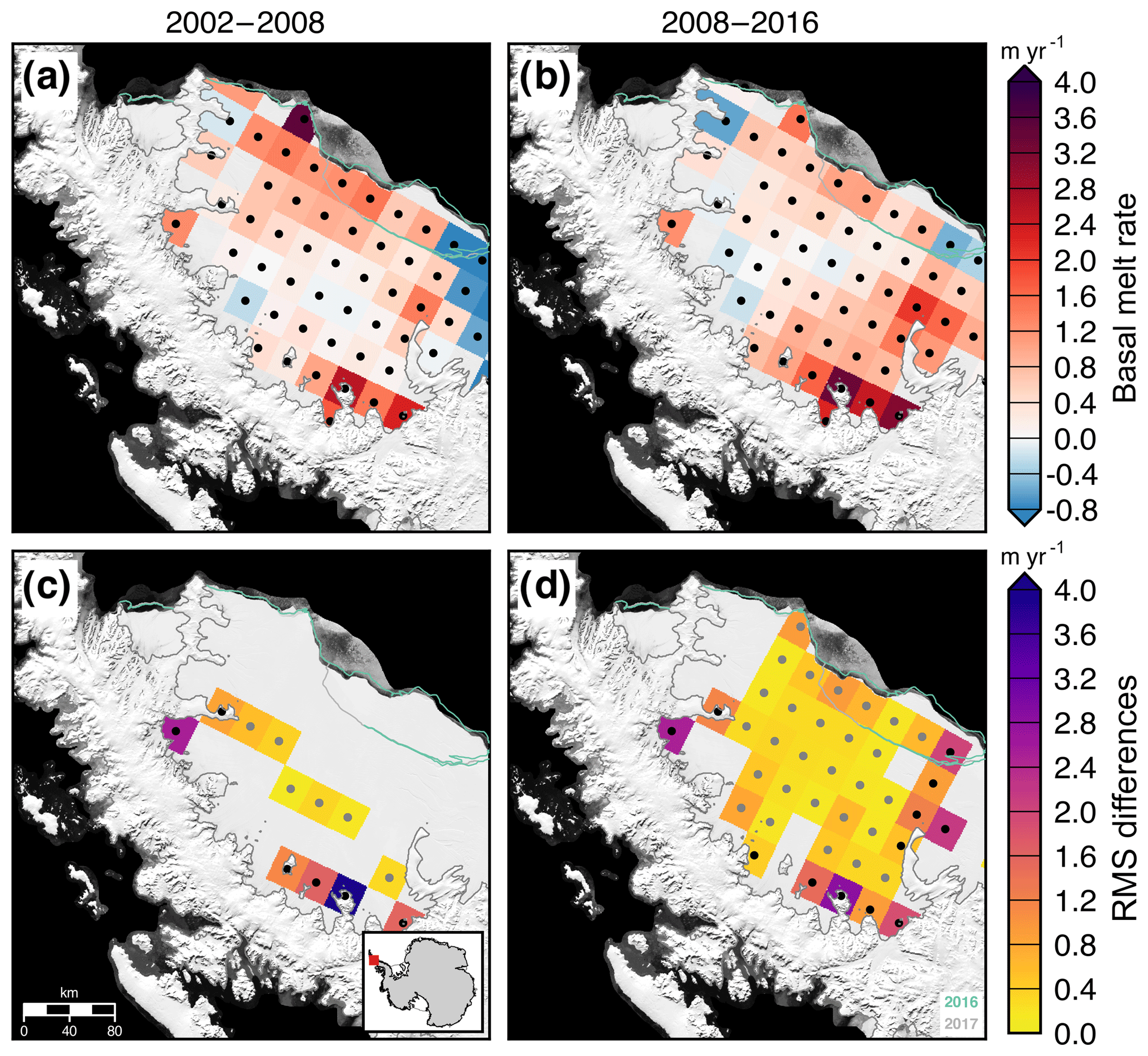
Figure 7Estimated basal melt rates (a–b) using radar altimetry from Adusumilli et al. (2018) and differences from melt rates derived from NASA–CECS Pre-IceBridge and NASA Operation IceBridge (c–d) of the Larsen-C Ice Shelf for two periods, 2002–2008 and 2008–2016. Stipples indicate locations with valid radar altimetry data (a–b) and coincident airborne laser altimetry data (c–d). MEaSUREs InSAR-derived Antarctic grounded ice boundaries are denoted in gray (Mouginot et al., 2017b). The 2016 and 2017 ice shelf extents delineated from MODIS imagery are denoted in green and light gray, respectively (Scambos et al., 2001). Plots are overlaid on a 2008–2009 MODIS mosaic of Antarctica (Haran et al., 2014). The inset map denotes the location of the maps.
2.2.2 Surface mass balance and firn compaction
After correcting for the effects of oceanic variation and advection, changes in surface height are due to a combination of accumulation, ablation, and firn densification processes. To account for variations in surface elevation due to changes in surface processes, we use monthly mean surface mass balance (SMB) outputs calculated from climate simulations of the Regional Atmospheric Climate Model (RACMO2.3p2) computed by the Ice and Climate group at the Institute for Marine and Atmospheric Research of Utrecht University (Ligtenberg et al., 2013; van Wessem et al., 2014, 2018). We use 5.5 km horizontal resolution outputs from a 1979–2016 climate simulation of the Antarctic Peninsula (XPEN055, van Wessem et al., 2016) and a 1979–2015 climate simulation of West Antarctica (ASE055, Lenaerts et al., 2018). The high-resolution outputs better represent the SMB state than outputs from the 27 km ice-sheet-wide model, particularly in the highly complex topography of mountains and glacial valleys in the Antarctic Peninsula (van Wessem et al., 2016). The higher spatial resolution topography improves the modeling of wind-driven downstream effects over ice shelves (Datta et al., 2018). SMB is the quantified difference between mass inputs from the precipitation of snow and rain, as well as mass losses by sublimation, runoff, and wind scour (Lenaerts et al., 2012; van den Broeke et al., 2009). Runoff is the portion of total snowmelt not retained or refrozen within the ice sheet. Wind scour is the erosion and sublimation of windblown snow from the ice sheet surface (Das et al., 2013). The absolute precision of the RACMO2.3p2 model outputs has been estimated using NASA Operation IceBridge snow radar observations, satellite observations of surface melt, and in situ observations, such as ice cores and surface stake measurements, following Kuipers Munneke et al. (2017) and Lenaerts et al. (2018). To correct for variations in the firn layer thickness, we use air content outputs from a semiempirical firn densification model that simulates the steady-state firn density profile (Ligtenberg et al., 2011, 2012). The firn densification model is forced with SMB outputs, surface temperatures fields, and near-surface wind speed fields computed by RACMO2.3p2 (Ligtenberg et al., 2011). We assume a 15 % uncertainty in SMB and firn air content height change following estimates from Kuipers Munneke et al. (2017).
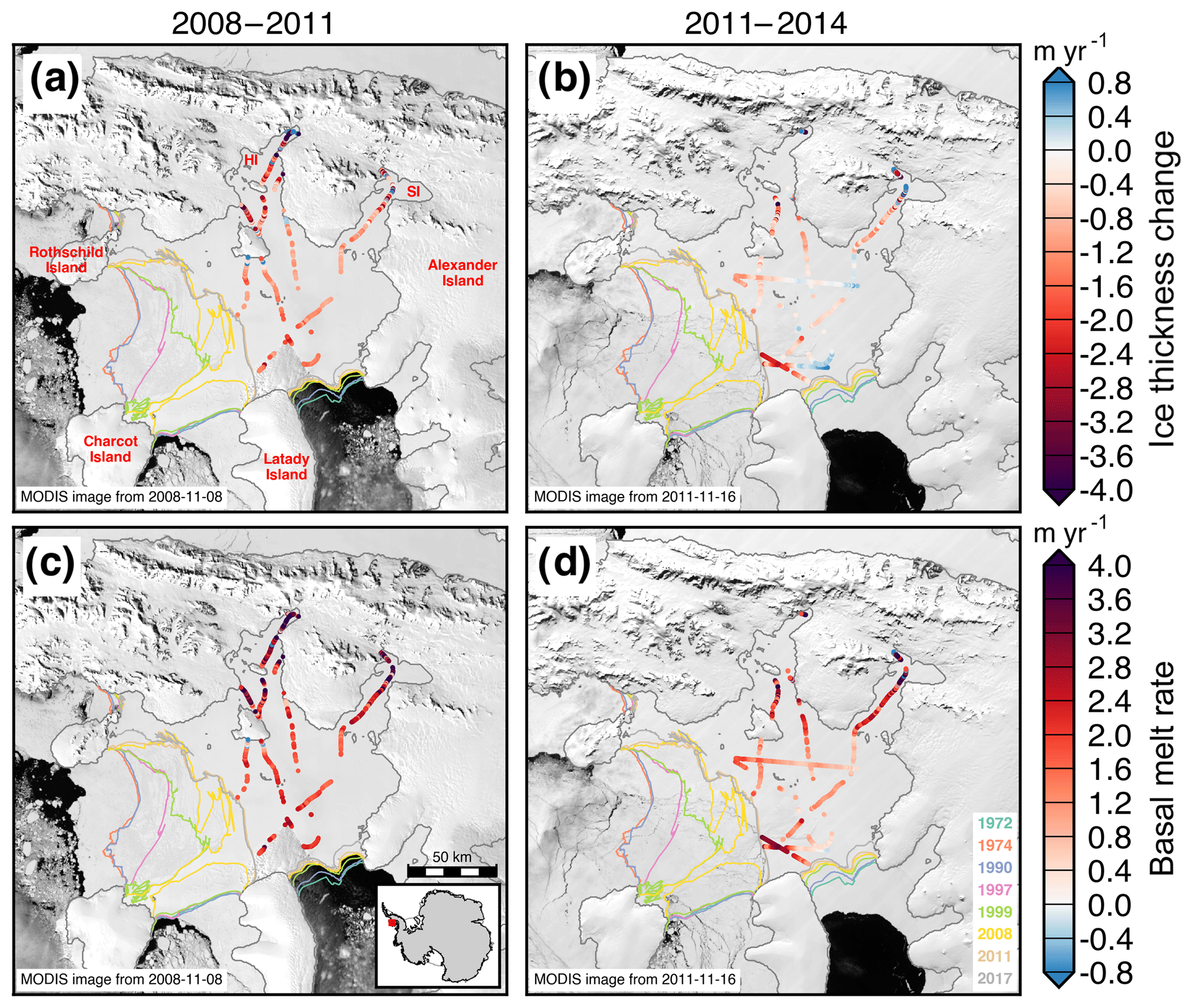
Figure 8Ice thickness change (a–b) and estimated basal melt rates (c–d) of the Wilkins Ice Shelf for two periods, 2008–2011 and 2011–2014. HI and SI denote the Haydn and Schubert inlets, respectively. MEaSUREs InSAR-derived Antarctic grounded ice boundaries are denoted in gray (Mouginot et al., 2017b). Historical ice shelf extents delineated from Landsat and MODIS imagery are denoted with colored lines. Plots are overlaid on MODIS images of Antarctic ice shelves provided by NSIDC (Scambos et al., 2001). The inset map denotes the location of the maps.
2.3 Ice shelf bottom melt
Changes in ice shelf mass in a Lagrangian reference frame are due to changes in SMB processes (Ms), basal melt (Mb), and the divergence of the ice shelf flow field (M∇⋅V) (Moholdt et al., 2014).
where hoc represent ocean heights, and hfc represent firn-column air content heights. We estimate ice shelf bottom melt rates along flight lines by using mass conservation and estimates of the mass flux divergence (Rignot and Jacobs, 2002; Moholdt et al., 2014; Rignot et al., 2013). Ice flow divergence fields are calculated from ice velocities from Rignot et al. (2017) differentiated using a Savitzky–Golay filter with an 11 km half-width window (Savitzky and Golay, 1964). The Savitzky–Golay algorithm smooths the velocity field and reduces the impact of ionospheric noise and other sources of uncertainty on the differentials. Deviations from mean ice flow were calculated using annually resolved ice velocity maps derived from synthetic aperture radar and optical imagery (Mouginot et al., 2017a). Ice shelf masses, M, were calculated by converting the altimetry-derived ice shelf freeboard heights, h, to ice thickness, H, by assuming hydrostatic equilibrium (Fricker et al., 2001; Griggs and Bamber, 2011).
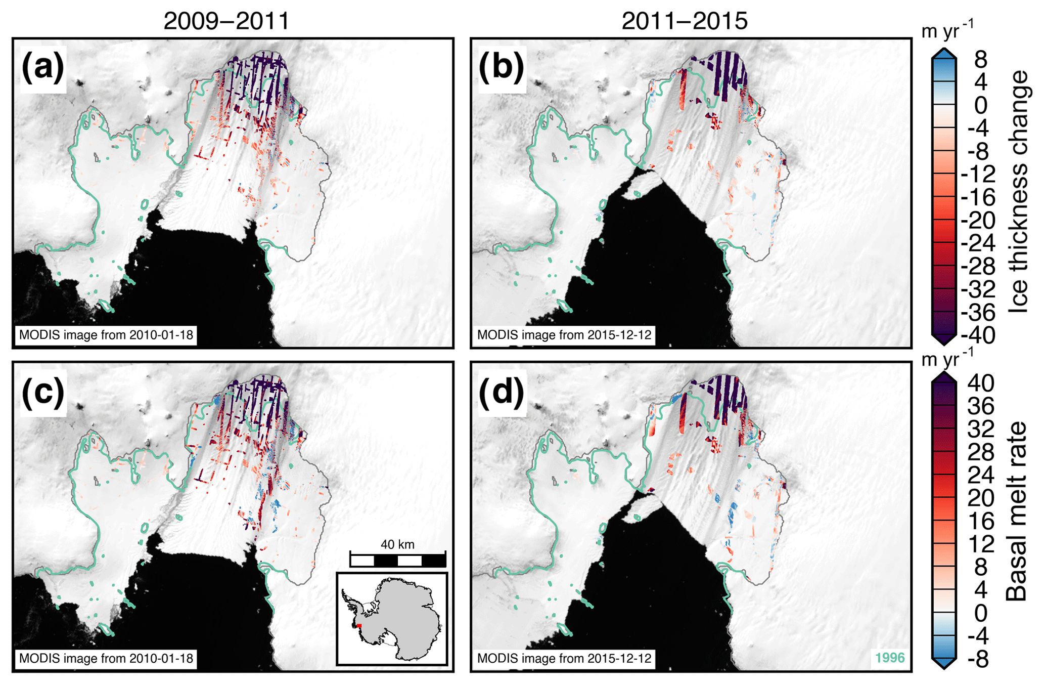
Figure 9Ice thickness change (a–b) and estimated basal melt rates (c–d) of the Pine Island Ice Shelf for two periods, 2009–2011 and 2011–2015. MEaSUREs InSAR-derived Antarctic grounded ice boundaries are denoted in gray (Mouginot et al., 2017b). The 1996 InSAR-derived grounding line locations from Rignot et al. (2016) are delineated in green. Plots are overlaid on MODIS images of Antarctic ice shelves provided by NSIDC (Scambos et al., 2001). The inset map denotes the location of the maps.
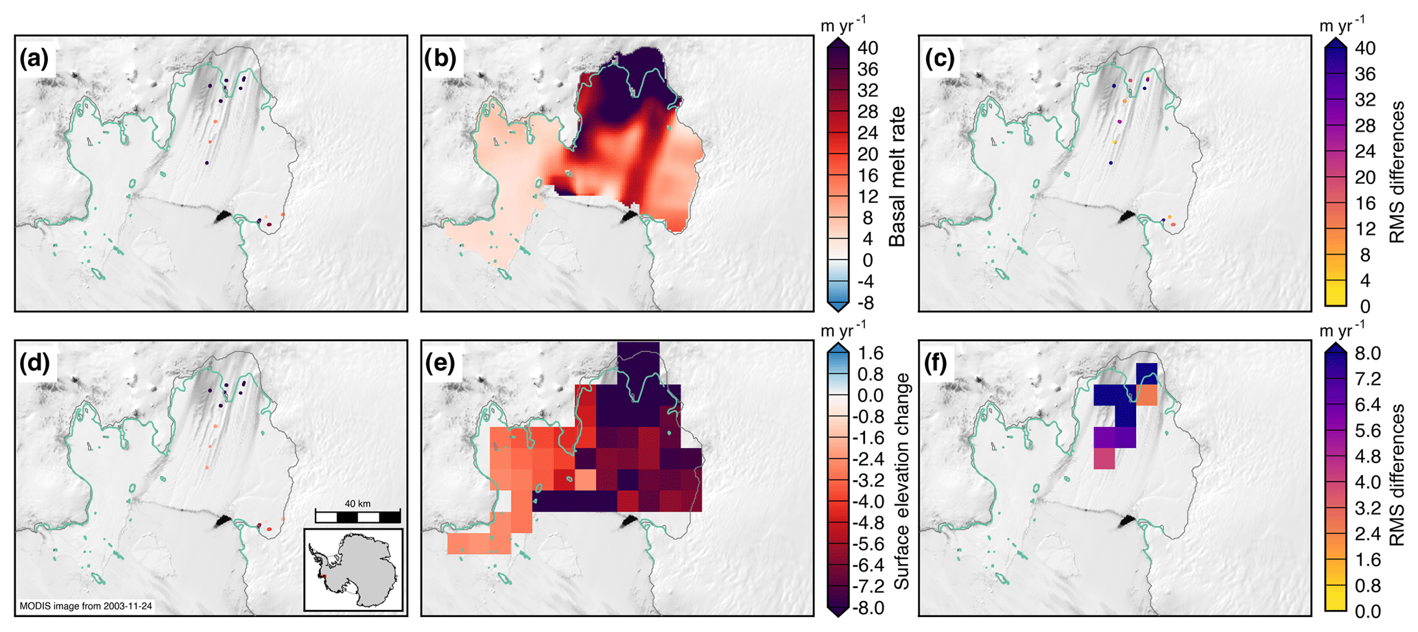
Figure 10Estimated basal melt rates (a–b) and differences in melt rates (c) of the Pine Island Ice Shelf from (a) NASA–CECS Pre-IceBridge and NASA Operation IceBridge over 2002–2009 and (b) from ICESat over 2003–2009 (Rignot et al., 2013). Estimated elevation change rates (d–e) and differences in elevation change rates (f) of the Pine Island Ice Shelf from (d) NASA–CECS Pre-IceBridge and NASA Operation IceBridge over 2002–2009 and (e) from ICESat over 2003–2009 after correcting for strain (Pritchard et al., 2012). MEaSUREs InSAR-derived Antarctic grounded ice boundaries are denoted in gray (Mouginot et al., 2017b). The 1996 InSAR-derived grounding line locations from Rignot et al. (2016) are delineated in green. Plots are overlaid on MODIS images of Antarctic ice shelves provided by NSIDC (Scambos et al., 2001). The inset map denotes the location of the maps.
We coregister 134 d of ATM data and 32 d of LVIS data for the years 2002–2016. We compare elevation change measurements between Eulerian and Lagrangian approaches derived using triangulated irregular networks (Sutterley et al., 2018, Fig. 4). Using a Lagrangian reference frame can produce estimates of ice shelf elevation change with much less noise compared with a Eulerian reference frame (Moholdt et al., 2014, Fig. 4). This is because the advection of ice thickness gradients, such as that from cracks and crevasses in the ice, can saturate the Eulerian-derived estimates (Moholdt et al., 2014; Shean et al., 2018).
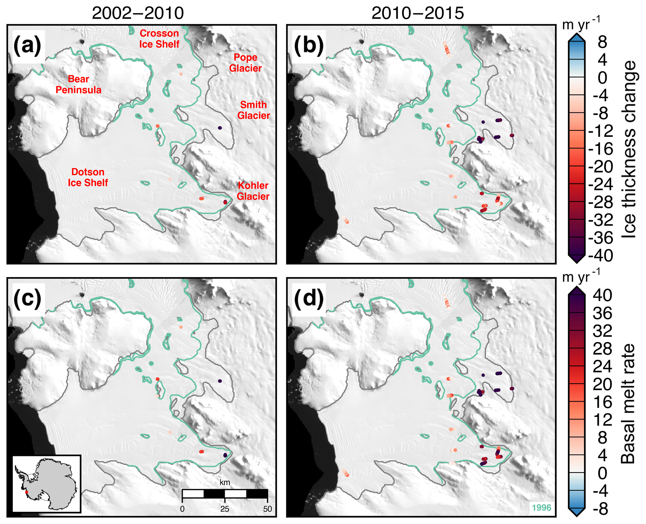
Figure 11Ice thickness change (a–b) and estimated basal melt rates (c–d) of the Dotson and Crosson ice shelves for two periods, 2002–2010 and 2010–2015. MEaSUREs InSAR-derived Antarctic grounded ice boundaries are denoted in gray (Mouginot et al., 2017b). The 1996 InSAR-derived grounding line locations from Rignot et al. (2016) are delineated in green. Plots are overlaid on a 2008–2009 MODIS mosaic of Antarctica (Haran et al., 2014). The inset map denotes the location of the maps.
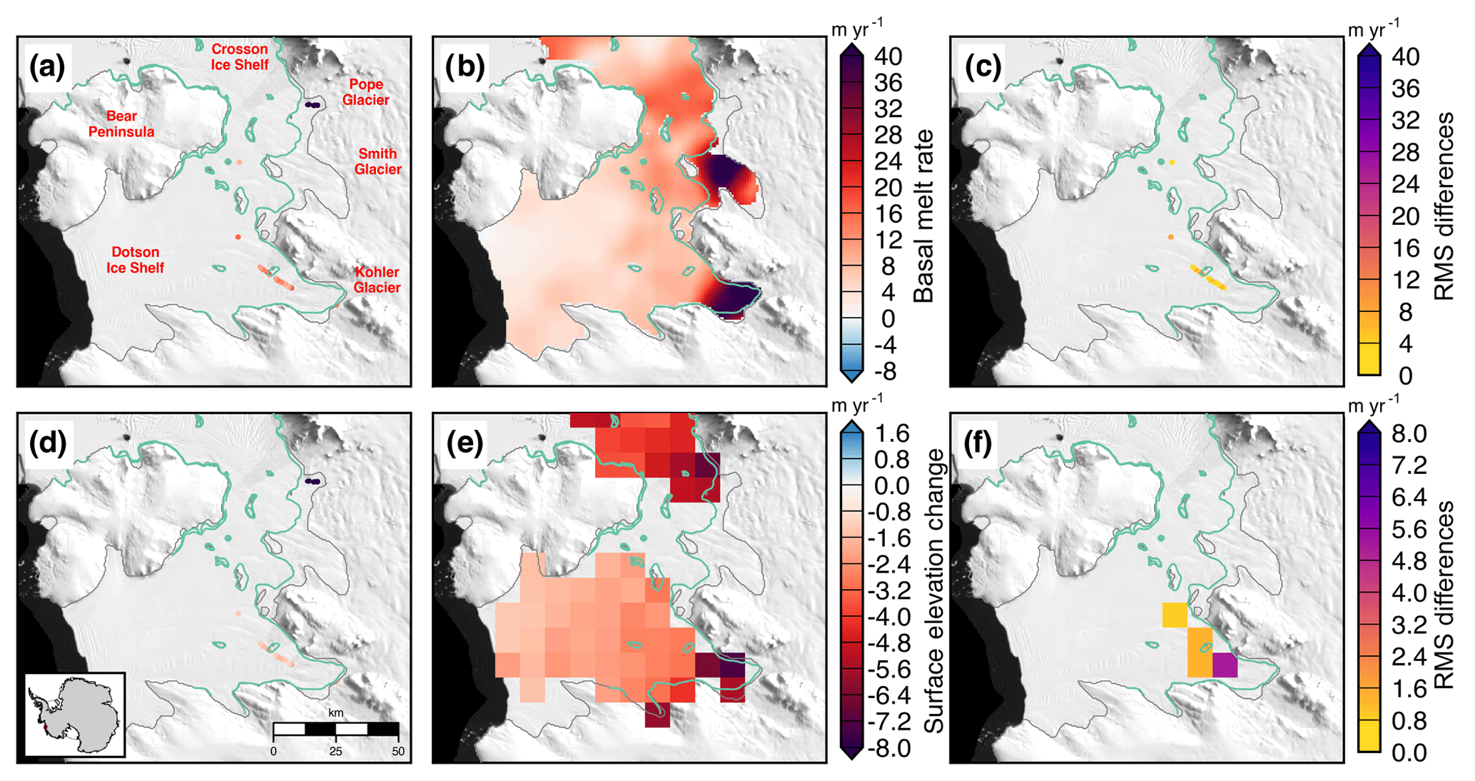
Figure 12Estimated basal melt rates (a–b) and differences in melt rates (c) of the Dotson and Crosson ice shelves from (a) NASA–CECS Pre-IceBridge and NASA Operation IceBridge over 2002–2009 and (b) from ICESat over 2003–2009 (Rignot et al., 2013). Estimated elevation change rates (d–e) and differences in elevation change rates (f) of the Dotson and Crosson ice shelves from (d) NASA–CECS Pre-IceBridge and NASA Operation IceBridge over 2002–2009 and (e) from ICESat over 2003–2009 after correcting for strain (Pritchard et al., 2012). MEaSUREs InSAR-derived Antarctic grounded ice boundaries are denoted in gray (Mouginot et al., 2017b). The 1996 InSAR-derived grounding line locations from Rignot et al. (2016) are delineated in green. Plots are overlaid on a 2008–2009 MODIS mosaic of Antarctica (Haran et al., 2014). The inset map denotes the location of the maps.
3.1 Larsen ice shelves
The ice shelves draining from the Antarctic Peninsula into the Weddell Sea have undergone some significant changes over the past three decades. The Larsen-A Ice Shelf collapsed in 1995, and the Larsen-B Ice Shelf partially collapsed in 2002 (Rott et al., 2002, 2011). The tributary glaciers once flowing into these shelves accelerated with the loss of the ice shelf abutment (Rignot et al., 2008). We estimate the impact of surface processes, ice divergence, and basal melt using data from a flight line starting near the Whirlwind Inlet of the Larsen-C Ice Shelf (Fig. 5a). Scatter in the Lagrangian-derived ice thickness change, DH∕Dt, across the flight line is typically 30–50 cm yr−1, or a 4–6 cm yr−1 error in the measured elevation change rate (Fig. 5a). Most of the thickness change, DH∕Dt, along this line is due to the flux divergence of the shelf, indicating the shelf along this line is nearly in steady state during this period. As the basal melt rate is calculated via mass conservation and the estimated DH∕Dt rate largely matches the flux divergence, estimates of the basal melt rate of the Larsen-C Ice Shelf are highly dependent on the SMB flux estimate. Any uncertainties in reconstructing the regional SMB will significantly impact the resultant basal melt rate estimate. The DH∕Dt rate of the Larsen-B remnant and Larsen-C ice shelves for two periods, 2002–2008 and 2008–2016, from NASA–CECS Pre-IceBridge and NASA Operation IceBridge airborne data is shown in Fig. 6a–b. The estimated basal melt rate of the ice shelves over the same periods is shown in Fig. 6c–d. The average DH∕Dt rate between 2008 and 2016 from the flight line data over the Larsen-C Ice Shelf is m yr−1. From 2008 to 2016, the strongest DH∕Dt rates occur near the grounding zone, particularly for the flight lines starting near Cabinet and Mill inlets. We compare our airborne laser altimetry estimate of basal melt rates with a long-term record derived from radar altimetry (Adusumilli et al., 2018). We find that the radar-derived estimate is comparable with the laser-derived estimate within uncertainties for most points outside of the grounding zone (Fig. 7). However, due to the sensitivity of the laser altimetry estimate to the SMB estimate (Fig. 5a), measurements from radar altimetry may be more accurate determinations of basal melt rate for the ice shelf.
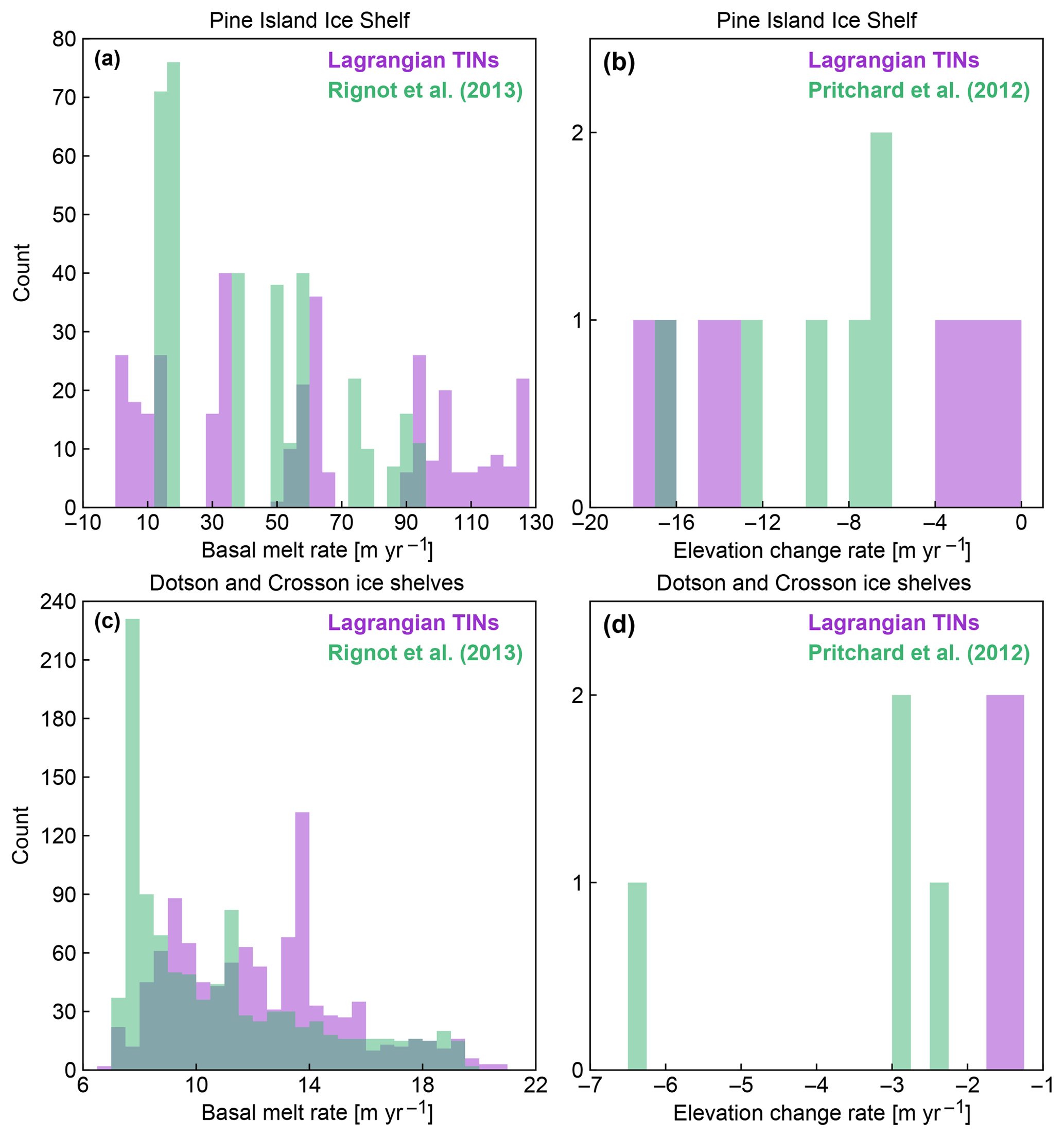
Figure 13Histograms of basal melt rates (a, c) and surface elevation change (b, d) of the Pine Island Ice Shelf (a, b) and Dotson and Crosson ice shelves (c, d) from NASA–CECS Pre-IceBridge and NASA Operation IceBridge over 2002–2009 (purple) and from ICESat over 2003–2009 (green) using data from Rignot et al. (2013) and Pritchard et al. (2012).
3.2 Wilkins Ice Shelf
The Wilkins Ice Shelf is fed by glaciers on Alexander Island, which is located near the west coast of the Antarctic Peninsula and is the largest of the Antarctic islands. The Wilkins Ice Shelf is sensitive to short-timescale coastal and upper-ocean processes (Padman et al., 2012) and ablates largely through basal melting (Rignot et al., 2013). DH∕Dt (a–b) and estimated basal melt rates (c–d) of the Wilkins Ice Shelf for two 3-year periods from 2008 to 2011 and from 2011 to 2014 are shown in Fig. 8. The extent of the ice shelf reduced from 16 000 to 10 000 km2 (38 %) between 1990 and 2017 (Scambos et al., 2009). The partial collapse occurred once the shelf started decoupling from Charcot Island (Vaughan et al., 1993) and likely occurred due to hydrofracturing (Scambos et al., 2009). Meltwater ponds covered areas of 300–600 km2 in Landsat imagery in 1986 and 1990 (Vaughan et al., 1993). The ponds existed largely in the now-collapsed portions of the shelf near Rothschild Island. Average DH∕Dt rates of the Wilkins Ice Shelf from the flight lines were m yr−1 from 2008 to 2011 and m yr−1 from 2011 to 2014. Average estimated basal melt rates from the flight lines were 2.5±1.3 m yr−1 in the earlier period and 1.8±0.9 m yr−1 in the latter period. Basal accretion could have occurred in some regions during the 2011–2014 period.
3.3 Pine Island Ice Shelf
The Pine Island Ice Shelf abuts one of the most rapidly changing glaciers in Antarctica (Pritchard et al., 2009; Flament and Rémy, 2012). Figure 9 shows the change in ice thickness (a–b) and estimated basal melt rates (c–d) of the Pine Island Ice Shelf for two periods from 2009 to 2011 and from 2011 to 2015. These periods were chosen to include repeat measurements from LVIS of the ice shelf near the grounding zone and to use the high-resolution outputs of RACMO2.3p2 ASE055. The average DH∕Dt rates from the flight lines were insignificantly different at m yr−1 over 2009–2011 and m yr−1 over 2011–2015. Because basal melt rates near the grounding zone have the highest impact on the glacial flow dynamics, we estimate the basal melt rate between the 1996 and 2011 grounding lines (Rignot and Jacobs, 2002). In this previously grounded region, the ice shelf DH∕Dt rates were m yr−1 during 2009–2011 and m yr−1 during 2011–2015. In this area that was previously grounded, the average estimated basal melt rates from the flight lines were 77±18 m yr−1 over 2009–2011 and 61±12 m yr−1 over 2011–2015. DH∕Dt rates outside of the previously grounded area between the 1996 and 2011 grounding lines are significantly smaller than in the previously grounded area, averaging m yr−1 for 2009–2011 and m yr−1 for 2011–2015. The difference in melt rates near the grounding zone between 2009–2011 and 2011–2015 could possibly explain some of the moderation in thinning of the grounded ice and stability in ice discharge from Pine Island Glacier after 2010 (McMillan et al., 2014; Medley et al., 2014). As shown in Fig. 9c–d, the DH∕Dt rate is dominated by strong submarine melt, which is further evidence of the dominant oceanic controls on the ice shelf mass balance in this region (Rignot, 2002; Shean et al., 2018). However, some of the changes in basal melt rate over the period could be due to large regional interannual-to-decadal variability (Dutrieux et al., 2014; Paolo et al., 2015; Jenkins et al., 2018). We compare our estimates of Pine Island Ice Shelf change from airborne laser altimetry with ICESat-derived surface elevation change from Pritchard et al. (2012) and basal melt rate from Rignot et al. (2013) (Figs. 10 and 13a–b). While there are few data points for comparison and the time periods are not contemporaneous (2002–2009 for the airborne data and 2003–2009 for the ICESat data), we find some significant differences between our airborne altimetry-derived estimates and the satellite-derived estimates (Fig. 10c, f). The rms differences between the airborne-derived estimate and the satellite-derived estimates are 31 m yr−1 in terms of basal melt rate (Rignot et al., 2013) and 8 m yr−1 in terms of surface elevation change (Pritchard et al., 2012). For the coincident data, the airborne altimetry data showed more variability in basal melt rate and surface elevation change than the satellite-derived methods (Fig. 13a–b). The differences in variability are likely due to the different spatial resolutions of the datasets, the different geophysical corrections applied for each estimate, and the spatial smoothing applied to the Pritchard et al. (2012) and Rignot et al. (2013) estimates.
3.4 Dotson and Crosson ice shelves
The glaciers flowing into the Dotson and Crosson ice shelves have rapidly thinned, increased in speed, and experienced significant retreats of grounding line positions over the past 20 years (Mouginot et al., 2014; Scheuchl et al., 2016). Flow speeds of the Crosson Ice Shelf have doubled in some regions over 1996 to 2014, while the flow speed of Dotson has remained largely steady (Lilien et al., 2018). DH∕Dt rates (a–b) and estimated basal melt rates (c–d) of the Dotson and Crosson ice shelves are shown in Fig. 11 for two periods, 2002–2010 and 2010–2015. Regions near the grounding lines of the input glaciers are decreasing in thickness rapidly for both shelves driven by strong basal melt. Basal melt rates averaged 47–81 m yr−1 near the grounding zone of Smith Glacier over the two periods. Khazendar et al. (2016) documented rapid submarine ice melt and the loss of 300–490 m of floating ice between 2002 and 2009. Our work here provides independent evidence of this large-scale melt using a separate method and more years of data. We find that the ice mass wastage continued unabated between 2010 and 2015 with DH∕Dt rates over the flight lines averaging m yr−1. We compare our airborne laser altimetry data of the Dotson and Crosson ice shelves with satellite laser altimetry estimates of surface elevation change from Pritchard et al. (2012) and basal melt rate from Rignot et al. (2013) (Figs. 12 and 13c–d). The rms differences between the airborne-derived estimate and the satellite-derived estimates are 5 m yr−1 in terms of basal melt rate (Rignot et al., 2013) and 4 m yr−1 in terms of surface elevation change (Pritchard et al., 2012). For the coincident data, the airborne altimetry data align well with the satellite-derived estimate of basal melt rate from Rignot et al. (2013) (Fig. 13c). However, the surface elevation estimates from Pritchard et al. (2012) do not align well with our airborne altimetry-derived estimate (Fig. 13d). The difference is likely due to the lack of spatial coverage with the airborne estimate, which may not be representative at the 10 km horizontal spatial scale of the Pritchard et al. (2012) estimate, particularly closer to the grounding line (Fig. 12f).
Using a Lagrangian reference frame may result in fewer coregistered data points and less spatial coverage of measurements compared with using an Eulerian reference frame (Fig. 4). Lagrangian tracking of airborne data requires (1) accurate flow-line flight planning, (2) a sufficiently wide scanning swath, or (3) dense grid measurements. Flight lines along flow need to be accurately planned to ensure upstream measurements can be paired with future downstream measurements. With the current airborne data at most locations, cross-flow flight lines advected outside of the swath width over multiyear repeat times. This limited our dataset to regions with flow-line measurements, such as the Larsen-C Ice Shelf (Fig. 6), or frequent measurements, such as the Dotson and Crosson ice shelves (Fig. 11). For most ice shelves, repeated airborne data are too sparse to extract large-scale spatial trends, particularly in the era before NASA Operation IceBridge. Satellite altimetry measurements from the NASA ICESat-2 mission (Markus et al., 2017) should help rectify the data limitation problem by providing dense and repeated point clouds. ICESat-2 data could be combined with photogrammetric digital elevation models (DEMs) to create high-resolution ice-shelf-wide thickness change maps (Berger et al., 2017; Shean et al., 2018). Combining ICESat-2 with DEMs would help improve the use of the laser altimetry data in a Lagrangian reference frame as ice parcels could be accurately tracked between separate satellite tracks. In addition, isolated crossovers can be calculated with the airborne data using Lagrangian tracking for some ice shelves using along-flow and cross-flow measurements from separate years. These singular crossovers would likely not be representative of the large-scale behavior of the ice shelf due to the spatial variability of ice thickness change but may still provide valuable metrics for evaluating outputs from ice sheet models (Figs. 10 and 12).
Lagrangian-derived estimates also greatly depend on the quality of the velocity estimates used for advecting the ice parcels in time. Here, the airborne data are coregistered in a Lagrangian reference frame using a static velocity map provided by NSIDC through the MEaSUREs program (Rignot et al., 2017). However, there are cases that do not fit the assumption of temporally invariant velocities. Prior to the calving event of the 40 000 km2 A-68 iceberg from the Larsen-C Ice Shelf on 11 July 2017, the ice was rifting from the south and the regions downstream of the crack were rotating outward (Hogg and Gudmundsson, 2017, Fig. 6). In the Amundsen Sea Embayment, the ice velocity structure has changed from year to year since the 1990s (Rignot et al., 2008; Mouginot et al., 2014). The floating ice shelves in the Amundsen Sea are also rifting concurrently with the acceleration of the instreaming glaciers (Macgregor et al., 2012). For both of these cases, it would be more appropriate to predict the advected parcel location using time-variable velocity maps. However, the spatial coverage of annual velocity maps is lacking for some time periods, which will complicate the advection calculation. For some locations, such as near shear margins, ice velocities can vary at smaller spatial scales than what is presently available from SAR measurements and visible imagery feature tracking. With the high-temporal-resolution data from the ESA Sentinel mission, the Landsat-based goLIVE project, and the future NASA-ISRO SAR mission (NISAR), the advected parcel locations could be predicted with much greater accuracy for recent NASA Operation IceBridge campaigns and future altimetry missions (Fahnestock et al., 2016; Gardner et al., 2018; Mouginot et al., 2017a). Improvements in ice thickness and ice velocity estimates will also greatly improve estimates of flux divergence and as a consequence estimates of basal melt rates calculated using mass conservation (Berger et al., 2017; Adusumilli et al., 2018).
This work builds off of the work of Paolo et al. (2015) and Adusumilli et al. (2018) that used radar altimetry data to analyze the recent thinning and basal melt rates of ice shelves. Paolo et al. (2015) calculated changes in the ice thickness time series over an 18-year time period using a suite of satellite radar altimetry data compiled in an Eulerian frame of reference. They found that the overall volume loss of ice shelves accelerated over the period 1994–2012, particularly for the ice shelves of West Antarctica. Adusumilli et al. (2018) expanded on this work by including radar altimetry data from CryoSat-2 to estimate the basal melt rates in the Antarctic Peninsula over a 23-year period. Laser altimeters and radar altimeters can measure different surfaces over snow-covered ice surfaces (Rémy and Parouty, 2009). Idealistically, the laser altimeter will detect the snow surface and the radar altimeter will detect the snow–ice interface. Because laser altimeters ideally detect the snow surface, an estimate of the total column snow/firn height change is needed to calculate the ice shelf freeboard change (Pritchard et al., 2012). For radar altimeters, the radar penetration depth is affected by variations in the dielectric properties of the surface layer due to variations in temperature, snow grain size, snow density, and moisture content (Partington et al., 1989; Rémy and Parouty, 2009). Due to the variations in penetration depth, estimates of the firn height change below the detected surface are necessary in order to calculate the freeboard change. Determining the sensitivity of radar estimates to surface penetration over different surface types could help reconcile differences between the various estimates (Fig. 7). In addition, in regions of uncertain SMB and firn change, intercomparisons with radar altimetry estimates may help provide important metrics for improving SMB and firn models. In these regions, radar altimetry estimates of ice thickness change may be more accurate than from laser altimetry due to the SMB uncertainty.
Compiling estimates of elevation change from laser altimetry is nontrivial, and different processing methods can produce differing results. Felikson et al. (2017) compared four different processing schemes (crossover differencing, along-track surface fits, overlapping footprints, and triangulated irregular networks) using ICESat data in an Eulerian sense over grounded ice in Greenland. They found discernible and irreconcilable differences between methods when deriving elevation change over the grounded ice sheet. We compare results from overlapping footprints and triangulated irregular networks to test their correspondence over ice shelf surfaces. As the surface slopes on ice shelves are small, we find that overlapping footprints and TIN approaches produce similar estimates of elevation change with scanning lidars in Lagrangian frames of reference (Fig. 4). The overlapping footprint approach produces a slightly noisier but statistically similar estimate compared with the TIN approach and is a significantly simpler algorithm to implement.
We present a method for measuring ice shelf thickness change through the coregistration of NASA–CECS Antarctic ice mapping and NASA Operation IceBridge laser altimetry data in a Lagrangian reference frame. We use our method to detect changes in ice shelves in West Antarctica and the Antarctic Peninsula where the airborne data are available. We find that our method can be a significant improvement over Eulerian-derived estimates that may require substantial spatial averaging of the data to reduce the impact of noise. However, there are significant limitations when using airborne data for detecting ice shelf thickness change with Lagrangian tracking, particularly the lower spatial coverage and typical lack of repeat tracks over ice shelves. Data from the recently launched NASA ICESat-2 mission will help rectify these problems, particularly if combined with high-resolution photogrammetric digital elevation models.
NASA Operation IceBridge data are freely available from the National Snow and Ice Data Center (NSIDC) at http://nsidc.org/data/ILATM2/ (last access: 25 June 2018; Studinger, 2014) for the Level-2 ATM data and http://nsidc.org/data/ILVIS2/ (last access: 9 June 2016; Blair and Hofton, 2010) for the Level-2 LVIS data. NASA MEaSUREs INSAR-derived velocity maps are provided by NSIDC at https://nsidc.org/data/nsidc-0484 (last access: 24 April 2017; Rignot et al., 2017). Bedmap2 ice thicknesses are provided by the British Antarctic Survey at https://www.bas.ac.uk/project/bedmap-2/ (last access: 7 December 2017; Fretwell et al., 2013). CATS2008 tidal constituents are available from the Earth & Space Research institute at https://www.esr.org/research/polar-tide-models/ (last access: 5 September 2017; Padman et al., 2008). Dynamic atmospheric corrections are produced by the CLS Space Oceanography Division using the Mog2D model from Legos distributed by https://www.aviso.altimetry.fr/en/data/products/auxiliary-products/atmospheric-corrections.html (AVISO, last access: 30 March 2018; Carrère and Lyard, 2003), with support from CNES. Ssalto/Duacs nontidal sea surface products were produced and distributed by the Copernicus Marine and Environment Monitoring Service (CMEMS; https://www.aviso.altimetry.fr/en/data/products/sea-surface-height-products/global/msla-h.html, last access: 7 July 2017; Le Traon et al., 1998). Landsat imagery is provided courtesy of the U.S. Geological Survey (EarthExplorer service, https://earthexplorer.usgs.gov/, last access: 11 May 2018; LPDAAC, 2017a, b, c, d, e). MODIS images of ice shelves are freely available from https://nsidc.org/data/iceshelves_images/index_modis.html (NSIDC, last access: 10 May 2018; Scambos et al., 2001). Altimetry data from this project are available on Figshare under a CC BY 4.0 license (https://doi.org/10.6084/m9.figshare.8159852, Sutterley et al., 2019). The following programs are provided by this project for processing the NASA Operation IceBridge data: nsidc-earthdata retrieves NASA data from NSIDC (https://doi.org/10.6084/m9.figshare.7355063, Sutterley, 2019a), read-ATM1b-QFIT-binary reads Level-1b Airborne Topographic Mapper (ATM) QFIT binary data products (https://doi.org/10.6084/m9.figshare.7355060, Sutterley, 2019b), read-ATM2-icessn reads Level-2 ATM Icessn data products (https://doi.org/10.6084/m9.figshare.7355066, Sutterley, 2019c), and read-LVIS2-elevation reads Level-2 Land Vegetation and Ice Sensor (LVIS) data products (https://doi.org/10.6084/m9.figshare.7355057, Sutterley, 2019d).
TCS performed the analysis and wrote the manuscript. TM and TAN supervised the project and provided comments and feedback. MvdB, SRML, and JMvW supplied the RACMO2.3p2 data and provided comments.
The authors declare that they have no conflict of interest.
We wish to thank Eric Rignot (UCI/JPL) and Isabella Velicogna (UCI/JPL) for their comments, as well as members of the GSFC Cryospheric Sciences Laboratory for their comments and advice. The authors thank Susheel Adusumilli (UCSD/SIO) for providing the estimated basal melt rates of the Larsen-C Ice Shelf from radar altimetry data, Hamish Pritchard (BAS) for providing the elevation change rates from ICESat altimetry data, and Jeremie Mouginot (IGE/UCI) for providing the estimated basal melt rates from ICESat altimetry data and his advice on the laser altimetry analysis. The authors wish to acknowledge the NASA Operation IceBridge flight, instrument, and science teams for their work to collect and produce the science data. We also wish to thank the National Snow and Ice Data Center (NSIDC) for storing and distributing the data from the NASA–CECS Antarctic ice mapping campaigns and NASA Operation IceBridge.
This research has been supported by an appointment to the NASA Postdoctoral Program at NASA Goddard Space Flight Center, administered by Universities Space Research Association under contract with NASA.
This paper was edited by Kenichi Matsuoka and reviewed by Laurence Padman and one anonymous referee.
Adusumilli, S., Fricker, H. A., Siegfried, M. R., Padman, L., Paolo, F. S., and Ligtenberg, S. R. M.: Variable Basal Melt Rates of Antarctic Peninsula Ice Shelves, 1994–2016, Geophys. Res. Lett., 45, 4086–4095, https://doi.org/10.1002/2017GL076652, 2018. a, b, c, d, e
Altamimi, Z., Rebischung, P., Métivier, L., and Collilieux, X.: ITRF2014: A new release of the International Terrestrial Reference Frame modeling nonlinear station motions, J. Geophys. Res.-Solid Earth, 121, 6109–6131, https://doi.org/10.1002/2016JB013098, 2016. a
Armitage, T. W. K., Kwok, R., Thompson, A. F., and Cunningham, G.: Dynamic Topography and Sea Level Anomalies of the Southern Ocean: Variability and Teleconnections, J. Geophys. Res.-Oceans, 123, 613–630, https://doi.org/10.1002/2017JC013534, 2018. a
Berger, S., Drews, R., Helm, V., Sun, S., and Pattyn, F.: Detecting high spatial variability of ice shelf basal mass balance, Roi Baudouin Ice Shelf, Antarctica, The Cryosphere, 11, 2675–2690, https://doi.org/10.5194/tc-11-2675-2017, 2017. a, b
Berthier, E., Scambos, T. A., and Shuman, C. A.: Mass loss of Larsen B tributary glaciers (Antarctic Peninsula) unabated since 2002, Geophys. Res. Lett., 39, l13501, https://doi.org/10.1029/2012GL051755, 2012. a
Blair, J. B. and Hofton, M.: IceBridge LVIS L2 Geolocated Surface Elevation Product, NASA DAAC at the National Snow and Ice Data Center, Boulder, Colorado USA, https://doi.org/10.5067/OIKFGJNBM6OO, version 2, 2010. a, b, c
Blair, J. B., Rabine, D. L., and Hofton, M. A.: The Laser Vegetation Imaging Sensor: a medium-altitude, digitisation-only, airborne laser altimeter for mapping vegetation and topography, ISPRS J. Photogramm. Remote Sens., 54, 115–122, https://doi.org/10.1016/S0924-2716(99)00002-7, 1999. a
Brunt, K. M., Fricker, H. A., Padman, L., Scambos, T. A., and O'Neel, S.: Mapping the grounding zone of the Ross Ice Shelf, Antarctica, using ICESat laser altimetry, Ann. Glaciol., 51, 71–79, https://doi.org/10.3189/172756410791392790, 2010. a
Brunt, K. M., Fricker, H. A., and Padman, L.: Analysis of ice plains of the Filchner–Ronne Ice Shelf, Antarctica, using ICESat laser altimetry, J. Glaciol., 57, 965–975, https://doi.org/10.3189/002214311798043753, 2011. a
Carrère, L. and Lyard, F.: Modeling the barotropic response of the global ocean to atmospheric wind and pressure forcing – comparisons with observations, Geophys. Res. Lett., 30, 1275, https://doi.org/10.1029/2002GL016473, 2003. a, b
Church, J. A., White, N. J., Konikow, L. F., Domingues, C. M., Cogley, J. G., Rignot, E. J., Gregory, J. M., van den Broeke, M. R., Monaghan, A. J., and Velicogna, I.: Revisiting the Earth's sea-level and energy budgets from 1961 to 2008, Geophys. Res. Lett., 38, l18601, https://doi.org/10.1029/2011GL048794, 2011. a
Cuffey, K. M. and Paterson, W. S. B.: The Physics of Glaciers, Butterworth-Heinemann, Burlington, MA, 4th edn., available at: https://www.elsevier.com/books/the-physics-of-glaciers/cuffey/978-0-12-369461-4 (last access: 25 June 2019), 2010. a
Das, I., Bell, R. E., Scambos, T. A., Wolovick, M., Creyts, T. T., Studinger, M., Frearson, N., Nicolas, J. P., Lenaerts, J. T. M., and van den Broeke, M. R.: Influence of persistent wind scour on the surface mass balance of Antarctica, Nat. Geosci., 6, 367–371, https://doi.org/10.1038/ngeo1766, 2013. a
Datta, R. T., Tedesco, M., Agosta, C., Fettweis, X., Kuipers Munneke, P., and van den Broeke, M. R.: Melting over the northeast Antarctic Peninsula (1999–2009): evaluation of a high-resolution regional climate model, The Cryosphere, 12, 2901–2922, https://doi.org/10.5194/tc-12-2901-2018, 2018. a
Depoorter, M. A., Bamber, J. L., Griggs, J. A., Lenaerts, J. T. M., Ligtenberg, S. R. M., van den Broeke, M. R., and Moholdt, G.: Calving fluxes and basal melt rates of Antarctic ice shelves, Nature, 502, 89–92, https://doi.org/10.1038/nature12567, 2013. a
Desai, S. D.: Observing the pole tide with satellite altimetry, J. Geophys. Res.-Oceans, 107, 7-1–7-13, https://doi.org/10.1029/2001JC001224, 2002. a
Dupont, T. and Alley, R. B.: Assessment of the importance of ice-shelf buttressing to ice-sheet flow, Geophys. Res. Lett., 32, l04503, https://doi.org/10.1029/2004GL022024, 2005. a
Dutrieux, P., De Rydt, J., Jenkins, A., Holland, P. R., Ha, H. K., Lee, S. H., Steig, E. J., Ding, Q., Abrahamsen, E., and Schröder, M.: Strong Sensitivity of Pine Island Ice-Shelf Melting to Climatic Variability, Science, 343, 174–178, https://doi.org/10.1126/science.1244341, 2014. a
Fahnestock, M., Scambos, T., Moon, T., Gardner, A., Haran, T., and Klinger, M.: Rapid large-area mapping of ice flow using Landsat 8, Remote Sens. Environ., 185, 84–94, https://doi.org/10.1016/j.rse.2015.11.023, 2016. a
Felikson, D., Urban, T. J., Gunter, B. C., Pie, N., Pritchard, H. D., Harpold, R., and Schutz, B. E.: Comparison of Elevation Change Detection Methods From ICESat Altimetry Over the Greenland Ice Sheet, IEEE Trans. Geosci. Remote Sens., 55, 1–12, https://doi.org/10.1109/TGRS.2017.2709303, 2017. a
Flament, T. and Rémy, F.: Dynamic thinning of Antarctic glaciers from along-track repeat radar altimetry, J. Glaciol., 58, 830–840, https://doi.org/10.3189/2012JoG11J118, 2012. a, b
Fretwell, P., Pritchard, H. D., Vaughan, D. G., Bamber, J. L., Barrand, N. E., Bell, R. E., Bianchi, C., Bingham, R. G., Blankenship, D. D., Casassa, G., Catania, G. A., Callens, D., Conway, H., Cook, A. J., Corr, H. F. J., Damaske, D., Damm, V., Ferraccioli, F., Forsberg, R., Fujita, S., Gim, Y., Gogineni, S. P., Griggs, J. A., Hindmarsh, R. C. A., Holmlund, P., Holt, J. W., Jacobel, R. W., Jenkins, A., Jokat, W., Jordan, T. A., King, E. C., Kohler, J., Krabill, W. B., Riger-Kusk, M., Langley, K. A., Leitchenkov, G., Leuschen, C., Luyendyk, B. P., Matsuoka, K., Mouginot, J., Nitsche, F. O., Nogi, Y., Nost, O. A., Popov, S. V., Rignot, E. J., Rippin, D. M., Rivera, A., Roberts, J. L., Ross, N., Siegert, M. J., Smith, A. M., Steinhage, D., Studinger, M., Sun, B., Tinto, B. K., Welch, B. C., Wilson, D., Young, D. A., Xiangbin, C., and Zirizzotti, A.: Bedmap2: improved ice bed, surface and thickness datasets for Antarctica, The Cryosphere, 7, 375–393, https://doi.org/10.5194/tc-7-375-2013, 2013. a, b
Fricker, H. A. and Padman, L.: Thirty years of elevation change on Antarctic Peninsula ice shelves from multimission satellite radar altimetry, J. Geophys. Res.-Oceans, 117, c02026, https://doi.org/10.1029/2011JC007126, 2012. a
Fricker, H. A., Popov, S., Allison, I., and Young, N.: Distribution of marine ice beneath the Amery Ice Shelf, Geophys. Res. Lett., 28, 2241–2244, https://doi.org/10.1029/2000GL012461, 2001. a, b
Gagliardini, O., Durand, G., Zwinger, T., Hindmarsh, R. C. A., and Le Meur, E.: Coupling of ice-shelf melting and buttressing is a key process in ice-sheets dynamics, Geophys. Res. Lett., 37, L145501, https://doi.org/10.1029/2010GL043334, 2010. a
Gardner, A. S., Moholdt, G., Scambos, T., Fahnstock, M., Ligtenberg, S., van den Broeke, M., and Nilsson, J.: Increased West Antarctic and unchanged East Antarctic ice discharge over the last 7 years, The Cryosphere, 12, 521–547, https://doi.org/10.5194/tc-12-521-2018, 2018. a
Goldberg, D., Holland, D. M., and Schoof, C.: Grounding line movement and ice shelf buttressing in marine ice sheets, J. Geophys. Res.-Earth Surf., 114, f04026, https://doi.org/10.1029/2008JF001227, 2009. a
Griggs, J. A. and Bamber, J. L.: Antarctic ice-shelf thickness from satellite radar altimetry, J. Glaciol., 57, 485–498, https://doi.org/10.3189/002214311796905659, 2011. a, b, c
Gudmundsson, G. H.: Ice-shelf buttressing and the stability of marine ice sheets, The Cryosphere, 7, 647–655, https://doi.org/10.5194/tc-7-647-2013, 2013. a
Haran, T., Bohlander, J., Scambos, T., and Fahnestock, M.: MODIS Mosaic of Antarctica 2008–2009 (MOA2009) Image Map, NSIDC: National Snow and Ice Data Center, Boulder, Colorado USA, https://doi.org/10.7265/N5KP8037, version 1, 2014. a, b, c, d, e, f, g
Hofton, M. A., Blair, J. B., Luthcke, S. B., and Rabine, D. L.: Assessing the performance of 20–25 m footprint waveform lidar data collected in ICESat data corridors in Greenland, Geophys. Res. Let., 35, l24501, https://doi.org/10.1029/2008GL035774, 2008. a
Hogg, A. E. and Gudmundsson, G. H.: Impacts of the Larsen-C Ice Shelf calving event, Nat. Clim. Change, 7, 540, https://doi.org/10.1038/nclimate3359, 2017. a
Jacobs, S. S., Jenkins, A., Giulivi, C. F., and Dutrieux, P.: Stronger ocean circulation and increased melting under Pine Island Glacier ice shelf, Nat. Geosci., 4, 519–523, https://doi.org/10.1038/ngeo1188, 2011. a
Jenkins, A., Shoosmith, D., Dutrieux, P., Jacobs, S., Kim, T. W., Lee, S. H., Ha, H. K., and Stammerjohn, S.: West Antarctic Ice Sheet retreat in the Amundsen Sea driven by decadal oceanic variability, Nat. Geosci., 11, 733–738, https://doi.org/10.1038/s41561-018-0207-4, 2018. a
Khazendar, A., Rignot, E. J., Schroeder, D. M., Seroussi, H., Schodlok, M. P., Scheuchl, B., Mouginot, J., Sutterley, T. C., and Velicogna, I.: Rapid submarine ice melting in the grounding zones of ice shelves in West Antarctica, Nat. Commun., 7, 13243, https://doi.org/10.1038/ncomms13243, 2016. a
King, M. A., Padman, L., Nicholls, K., Clarke, P. J., Gudmundsson, G., Kulessa, B., and Shepherd, A.: Ocean tides in the Weddell Sea: New observations on the Filchner-Ronne and Larsen C ice shelves and model validation, J. Geophys. Res.-Oceans, 116, c06006, https://doi.org/10.1029/2011JC006949, 2011. a
Kuipers Munneke, P., McGrath, D., Medley, B., Luckman, A., Bevan, S., Kulessa, B., Jansen, D., Booth, A., Smeets, P., Hubbard, B., Ashmore, D., Van den Broeke, M., Sevestre, H., Steffen, K., Shepherd, A., and Gourmelen, N.: Observationally constrained surface mass balance of Larsen C ice shelf, Antarctica, The Cryosphere, 11, 2411–2426, https://doi.org/10.5194/tc-11-2411-2017, 2017. a, b
Lenaerts, J. T. M., van den Broeke, M. R., van de Berg, W. J., van Meijgaard, E., and Kuipers Munneke, P.: A new, high-resolution surface mass balance map of Antarctica (1979–2010) based on regional atmospheric climate modeling, Geophys. Res. Lett., 39, l04501, https://doi.org/10.1029/2011GL050713, 2012. a
Lenaerts, J. T. M., Ligtenberg, S. R. M., Medley, B., Van de Berg, W. J., Konrad, H., Nicolas, J. P., Van Wessem, J. M., Trusel, L. D., Mulvaney, R., Tuckwell, R. J., Hogg, A. E., and Thomas, E. R.: Climate and surface mass balance of coastal West Antarctica resolved by regional climate modelling, Ann. Glaciol., 59, 29–41, https://doi.org/10.1017/aog.2017.42, 2018. a, b
Le Traon, P. Y., Nadal, F., and Ducet, N.: An Improved Mapping Method of Multisatellite Altimeter Data, J. Atmos. Ocean. Technol., 15, 522–534, https://doi.org/10.1175/1520-0426(1998)015<0522:AIMMOM>2.0.CO;2, 1998. a, b
Ligtenberg, S. R. M., Helsen, M. M., and van den Broeke, M. R.: An improved semi-empirical model for the densification of Antarctic firn, The Cryosphere, 5, 809–819, https://doi.org/10.5194/tc-5-809-2011, 2011. a, b, c
Ligtenberg, S. R. M., Horwath, M., van den Broeke, M. R., and Legrésy, B.: Quantifying the seasonal “breathing” of the Antarctic ice sheet, Geophys. Res. Lett., 39, l23501, https://doi.org/10.1029/2012GL053628, 2012. a
Ligtenberg, S. R. M., Berg, W. J., van den Broeke, M. R., Rae, J. G. L., and van Meijgaard, E.: Future surface mass balance of the Antarctic ice sheet and its influence on sea level change, simulated by a regional atmospheric climate model, Clim. Dynam., 41, 867–884, https://doi.org/10.1007/s00382-013-1749-1, 2013. a
Lilien, D. A., Joughin, I., Smith, B., and Shean, D. E.: Changes in flow of Crosson and Dotson ice shelves, West Antarctica, in, The Cryosphere, 12, 1415–1431, https://doi.org/10.5194/tc-12-1415-2018, 2018. a
LPDAAC: USGS EROS Archive – Landsat Archives – Landsat 8 OLI (Operational Land Imager) and TIRS (Thermal Infrared Sensor), NASA EOSDIS Land Processes Distributed Active Archive Center (LP DAAC), USGS/Earth Resources Observation and Science (EROS) Center, Sioux Falls, South Dakota, https://doi.org/10.5066/F71835S6, 2017a. a
LPDAAC: USGS EROS Archive – Landsat Archives – Landsat 7 Enhanced Thematic Mapper Plus (ETM+) Level-1 Data Products, NASA EOSDIS Land Processes Distributed Active Archive Center (LP DAAC), USGS/Earth Resources Observation and Science (EROS) Center, Sioux Falls, South Dakota https://doi.org/10.5066/F7WH2P8G, 2017b. a
LPDAAC: USGS EROS Archive – Landsat Archives – Landsat 4-5 Thematic Mapper (TM) Level-1 Data Products, NASA EOSDIS Land Processes Distributed Active Archive Center (LP DAAC), USGS/Earth Resources Observation and Science (EROS) Center, Sioux Falls, South Dakota, https://doi.org/10.5066/F7N015TQ, 2017c. a
LPDAAC: USGS EROS Archive – Landsat Archives – Landsat 1-5 Multispectral Scanner (MSS) Level-1 Data Products, NASA EOSDIS Land Processes Distributed Active Archive Center (LP DAAC), USGS/Earth Resources Observation and Science (EROS) Center, Sioux Falls, South Dakota, https://doi.org/10.5066/F7H994GQ, 2017d. a
LPDAAC: NASA Landsat Program, NASA EOSDIS Land Processes Distributed Active Archive Center (LP DAAC), USGS/Earth Resources Observation and Science (EROS) Center, Sioux Falls, South Dakota, available at: https://lpdaac.usgs.gov/ (last access: 31 May 2019), 2017e. a
Lynch, D. R. and Gray, W. G.: A wave equation model for finite element tidal computations, Comput. Fluid., 7, 207–228, https://doi.org/10.1016/0045-7930(79)90037-9, 1979. a
Macgregor, J. A., Catania, G. A., Markowski, M. S., and Andrews, A. G.: Widespread rifting and retreat of ice-shelf margins in the eastern Amundsen Sea Embayment between 1972 and 2011, J. Glaciol., 58, 458–466, https://doi.org/10.3189/2012JoG11J262, 2012. a
Markus, T., Neumann, T., Martino, A., Abdalati, W., Brunt, K., Csatho, B., Farrell, S., Fricker, H., Gardner, A., Harding, D., Jasinski, M., Kwok, R., Magruder, L., Lubin, D., Luthcke, S., Morison, J., Nelson, R., Neuenschwander, A., Palm, S., Popescu, S., Shum, C., Schutz, B. E., Smith, B., Yang, Y., and Zwally, J.: The Ice, Cloud, and land Elevation Satellite-2 (ICESat-2): Science requirements, concept, and implementation, Remote Sens. Environ., 190, 260–273, https://doi.org/10.1016/j.rse.2016.12.029, 2017. a, b, c
McMillan, M., Shepherd, A., Sundal, A. V., Briggs, K. H., Muir, A., Ridout, A., Hogg, A., and Wingham, D.: Increased ice losses from Antarctica detected by CryoSat-2, Geophys. Res. Lett., 41, 3899–3905, https://doi.org/10.1002/2014GL060111, 2014. a
Medley, B., Joughin, I. R., Smith, B. E., Das, S. B., Steig, E. J., Conway, H., Gogineni, S. P., Lewis, C., Criscitiello, A. S., McConnell, J. R., van den Broeke, M. R., Lenaerts, J. T. M., Bromwich, D. H., Nicolas, J. P., and Leuschen, C.: Constraining the recent mass balance of Pine Island and Thwaites glaciers, West Antarctica, with airborne observations of snow accumulation, The Cryosphere, 8, 1375–1392, https://doi.org/10.5194/tc-8-1375-2014, 2014. a
Moholdt, G., Padman, L., and Fricker, H. A.: Basal mass budget of Ross and Filchner-Ronne ice shelves, Antarctica, derived from Lagrangian analysis of ICESat altimetry, J. Geophys. Res.-Earth Surf., 119, 2361–2380, https://doi.org/10.1002/2014JF003171, 2014. a, b, c, d, e, f, g
Mouginot, J., Rignot, E. J., and Scheuchl, B.: Sustained increase in ice discharge from the Amundsen Sea Embayment, West Antarctica, from 1973 to 2013, Geophys. Res. Lett., 41, 1576–1584, https://doi.org/10.1002/2013GL059069, 2014. a, b
Mouginot, J., Rignot, E., Scheuchl, B., and Millan, R.: Comprehensive Annual Ice Sheet Velocity Mapping Using Landsat-8, Sentinel-1, and RADARSAT-2 Data, Remote Sens., 9, 364, https://doi.org/10.3390/rs9040364, 2017a. a, b
Mouginot, J., Scheuchl, B., and Rignot, E.: MEaSUREs Antarctic Boundaries for IPY 2007–2009 from Satellite Radar, NASA National Snow and Ice Data Center Distributed Active Archive Center, Boulder, Colorado USA, https://doi.org/10.5067/AXE4121732AD, version 2, 2017b. a, b, c, d, e, f, g, h, i, j, k
Neumann, T., Brenner, A., Hancock, D., Robbins, J., and Saba, J.: Ice, Cloud, and land Elevation Satellite – 2 (ICESat-2) Project: Algorithm Theoretical Basis Document (ATBD) for Global Geolocated Photons (ATL03), Tech. rep., NASA Goddard Space Flight Center (GSFC), Greenbelt, MD, USA, available at: https://icesat-2.gsfc.nasa.gov/science/data-products (last access: 31 May 2019), 2018. a
Padman, L., Fricker, H. A., Coleman, R., Howard, S., and Erofeeva, L.: A new tide model for the Antarctic ice shelves and seas, Ann. Glaciol., 34, 247–254, https://doi.org/10.3189/172756402781817752, 2002. a
Padman, L., Erofeeva, S. Y., and Fricker, H. A.: Improving Antarctic tide models by assimilation of ICESat laser altimetry over ice shelves, Geophys. Res. Lett., 35, l22504, https://doi.org/10.1029/2008GL035592, 2008. a, b
Padman, L., Costa, D. P., Dinniman, M. S., Fricker, H. A., Goebel, M. E., Huckstadt, L. A., Humbert, A., Joughin, I. R., Lenaerts, J. T. M., Ligtenberg, S. R. M., Scambos, T. A., and van den Broeke, M. R.: Oceanic controls on the mass balance of Wilkins Ice Shelf, Antarctica, J. Geophys. Res.-Oceans, 117, c01010, https://doi.org/10.1029/2011JC007301, 2012. a
Paolo, F. S., Fricker, H. A., and Padman, L.: Volume loss from Antarctic ice shelves is accelerating, Science, 348, 327–331, https://doi.org/10.1126/science.aaa0940, 2015. a, b, c
Paolo, F. S., Fricker, H. A., and Padman, L.: Constructing improved decadal records of Antarctic ice shelf height change from multiple satellite radar altimeters, Remote Sens. Environ., 177, 192–205, https://doi.org/10.1016/j.rse.2016.01.026, 2016. a, b
Partington, K. C., Ridley, J. K., Rapley, C. G., and Zwally, H. J.: Observations of the Surface Properties of the Ice Sheets by Satellite Radar Altimetry, J. Glaciol., 35, 267–275, https://doi.org/10.3189/S0022143000004603, 1989. a
Petit, G. and Luzum, B.: IERS Conventions (2010), Tech. Rep. 36, International Earth Rotation and Reference Systems Service (IERS), Frankfurt am Main: Verlag des Bundesamts für Kartographie und Geodäsie, available at: https://www.iers.org/IERS/EN/Publications/TechnicalNotes/tn36.html (last access: 13 October 2017), 2010. a
Pritchard, H. D., Arthern, R. J., Vaughan, D. G., and Edwards, L. A.: Extensive dynamic thinning on the margins of the Greenland and Antarctic ice sheets, Nature, 461, 971–975, https://doi.org/10.1038/nature08471, 2009. a, b, c, d
Pritchard, H. D., Ligtenberg, S. R. M., Fricker, H. A., Vaughan, D. G., van den Broeke, M. R., and Padman, L.: Antarctic ice-sheet loss driven by basal melting of ice shelves, Nature, 484, 502–505, https://doi.org/10.1038/nature10968, 2012. a, b, c, d, e, f, g, h, i, j, k, l, m, n
Ray, R. D.: A global ocean tide model from Topex/Poseidon altimetry: GOT99.2, Tech. Rep. TM-1999-209478, NASA Goddard Space Flight Center, Greenbelt, MD, available at: http://ntrs.nasa.gov/archive/nasa/casi.ntrs.nasa.gov/19990089548_1999150788.pdf (last access: 22 September 2017), 1999. a
Rémy, F. and Parouty, S.: Antarctic Ice Sheet and Radar Altimetry: A Review, Remote Sensing, 1, 1212–1239, https://doi.org/10.3390/rs1041212, 2009. a, b
Ries, J., Bettadpur, S., Eanes, R., Kang, Z., Ko, U., McCullough, C., Nagel, P., Pie, N., Poole, S., Richter, T., Save, H., and Tapley, B.: The Development and Evaluation of the Global Gravity Model GGM05, Tech. Rep. CSR-16-02, UTCSR, Austin, Texas, https://doi.org/10.5880/icgem.2016.002, 2016. a
Rignot, E.: Ice-shelf changes in Pine Island Bay, Antarctica, 1947–2000, J. Glaciol., 48, 247–256, https://doi.org/10.3189/172756502781831386, 2002. a
Rignot, E. J. and Jacobs, S.: Rapid Bottom Melting Widespread near Antarctic Ice Sheet Grounding Lines, Science, 296, 2020–2023, https://doi.org/10.1126/science.1070942, 2002. a, b
Rignot, E. J., Vaughan, D. G., Schmeltz, M., Dupont, T., and MacAyeal, D. R.: Acceleration of Pine Island and Thwaites Glaciers, West Antarctica, Ann. Glaciol., 34, 189–194, https://doi.org/10.3189/172756402781817950, 2002. a
Rignot, E. J., Casassa, G., Gogineni, S. P., Krabill, W. B., Rivera, A., and Thomas, R. H.: Accelerated ice discharge from the Antarctic Peninsula following the collapse of Larsen B ice shelf, Geophys. Res. Lett., 31, l18401, https://doi.org/10.1029/2004GL020697, 2004. a
Rignot, E. J., Bamber, J. L., van den Broeke, M. R., Davis, C. H., Li, Y., van de Berg, W. J., and van Meijgaard, E.: Recent Antarctic ice mass loss from radar interferometry and regional climate modelling, Nat. Geosci., 1, 106–110, https://doi.org/10.1038/ngeo102, 2008. a, b, c
Rignot, E. J., Jacobs, S., Mouginot, J., and Scheuchl, B.: Ice-Shelf Melting Around Antarctica, Science, 341, 266–270, https://doi.org/10.1126/science.1235798, 2013. a, b, c, d, e, f, g, h, i, j, k, l, m, n
Rignot, E. J., Mouginot, J., Morlighem, M., Seroussi, H., and Scheuchl, B.: Widespread, rapid grounding line retreat of Pine Island, Thwaites, Smith, and Kohler glaciers, West Antarctica, from 1992 to 2011, Geophys. Res. Lett., 41, 3502–3509, https://doi.org/10.1002/2014GL060140, 2014. a
Rignot, E. J., Mouginot, J., and Scheuchl, B.: MEaSUREs Antarctic Grounding Line from Differential Satellite Radar Interferometry, NASA National Snow and Ice Data Center Distributed Active Archive Center, Boulder, Colorado USA, https://doi.org/10.5067/IKBWW4RYHF1Q, version 2, 2016. a, b, c, d, e
Rignot, E. J., Mouginot, J., and Scheuchl, B.: MEaSUREs InSAR-Based Antarctica Ice Velocity Map, NASA National Snow and Ice Data Center Distributed Active Archive Center, Boulder, Colorado USA, https://doi.org/10.5067/D7GK8F5J8M8R, version 2, 2017. a, b, c, d, e
Rott, H., Rack, W., Skvarca, P., and De Angelis, H.: Northern Larsen Ice Shelf, Antarctica: further retreat after collapse, Ann. Glaciol., 34, 277–282, https://doi.org/10.3189/172756402781817716, 2002. a
Rott, H., Müller, F., Nagler, T., and Floricioiu, D.: The imbalance of glaciers after disintegration of Larsen-B ice shelf, Antarctic Peninsula, The Cryosphere, 5, 125–134, https://doi.org/10.5194/tc-5-125-2011, 2011. a
Savitzky, A. and Golay, M. J. E.: Smoothing and Differentiation of Data by Simplified Least Squares Procedures., Anal. Chem., 36, 1627–1639, https://doi.org/10.1021/ac60214a047, 1964. a
Scambos, T., Raup, B. H., and Bohlander, J.: Images of Antarctic Ice Shelves, NASA National Snow and Ice Data Center Distributed Active Archive Center, Boulder, Colorado USA, https://doi.org/10.7265/N5NC5Z4N, version 1, 2001. a, b, c, d, e, f, g, h
Scambos, T., Fricker, H. A., Liu, C.-C., Bohlander, J., Fastook, J., Sargent, A., Massom, R., and Wu, A.-M.: Ice shelf disintegration by plate bending and hydro-fracture: Satellite observations and model results of the 2008 Wilkins ice shelf break-ups, Earth Planet. Sci. Lett., 280, 51–60, https://doi.org/10.1016/j.epsl.2008.12.027, 2009. a, b
Scheuchl, B., Mouginot, J., Rignot, E. J., Morlighem, M., and Khazendar, A.: Grounding line retreat of Pope, Smith, and Kohler Glaciers, West Antarctica, measured with Sentinel-1a radar interferometry data, Geophys. Res. Lett., 43, 8572–8579, https://doi.org/10.1002/2016GL069287, 2016. a
Shean, D. E., Joughin, I. R., Dutrieux, P., Smith, B. E., and Berthier, E.: Ice shelf basal melt rates from a high-resolution DEM record for Pine Island Glacier, Antarctica, The Cryosphere Discuss., https://doi.org/10.5194/tc-2018-209, in review, 2018. a, b, c, d
Shepherd, A., Wingham, D. J., Payne, T., and Skvarca, P.: Larsen Ice Shelf Has Progressively Thinned, Science, 302, 856–859, https://doi.org/10.1126/science.1089768, 2003. a
Slobbe, D. C., Lindenbergh, R. C., and Ditmar, P.: Estimation of volume change rates of Greenland's ice sheet from ICESat data using overlapping footprints, Remote Sens. Environ., 112, 4204–4213, https://doi.org/10.1016/j.rse.2008.07.004, 2008. a
Smith, B. E., Gourmelen, N., Huth, A., and Joughin, I.: Connected subglacial lake drainage beneath Thwaites Glacier, West Antarctica, The Cryosphere, 11, 451–467, https://doi.org/10.5194/tc-11-451-2017, 2017. a, b
Studinger, M. S.: IceBridge ATM L2 Icessn Elevation, Slope, and Roughness, NASA National Snow and Ice Data Center Distributed Active Archive Center, Boulder, Colorado USA, https://doi.org/10.5067/CPRXXK3F39RV, version 2, 2014. a, b, c
Sutterley, T. C., Velicogna, I., Fettweis, X., Rignot, E., Noël, B., and van den Broeke, M.: Evaluation of Reconstructions of Snow/Ice Melt in Greenland by Regional Atmospheric Climate Models Using Laser Altimetry Data, Geophys. Res. Lett., 45, 8324–8333, https://doi.org/10.1029/2018GL078645, 2018. a, b, c, d, e, f
Sutterley, T. C.: nsidc-earthdata,
https://doi.org/10.6084/m9.figshare.7355063, 2019a. a
Sutterley, T. C.: read-ATM1b-QFIT-binary,
https://doi.org/10.6084/m9.figshare.7355060, 2019b. a
Sutterley, T. C.: read-ATM2-icessn,
https://doi.org/10.6084/m9.figshare.7355066, 2019c. a
Sutterley, T. C.: read-LVIS2-elevation,
https://doi.org/10.6084/m9.figshare.7355057, 2019d. a
Sutterley, T. C., Markus, T., Neumann, T., van den Broeke, M., van Wessem, J. M., and Ligtenberg, S.: Antarctic Ice Shelf Thickness Change and Bottom Melt Rates from NASA/CECS Antarctic Ice Mapping and NASA Operation IceBridge, https://doi.org/10.6084/m9.figshare.8159852, 2019. a
Thomas, R. H.: Ice Shelves: A Review, J. Glaciol., 24, 273–286, https://doi.org/10.1017/S0022143000014799, 1979. a, b, c
Thomas, R. H. and Studinger, M. S.: Pre-IceBridge ATM L2 Icessn Elevation, Slope, and Roughness, NASA National Snow and Ice Data Center Distributed Active Archive Center, Boulder, Colorado USA, https://doi.org/10.5067/6C6WA3R918HJ, version 1, 2010. a, b
van den Broeke, M. R., Bamber, J. L., Ettema, J., Rignot, E. J., Schrama, E., van de Berg, W. J., van Meijgaard, E., Velicogna, I., and Wouters, B.: Partitioning Recent Greenland Mass Loss, Science, 326, 984–986, https://doi.org/10.1126/science.1178176, 2009. a
van Wessem, J. M., Reijmer, C. H., Morlighem, M., Mouginot, J., Rignot, E. J., Medley, B., Joughin, I. R., Wouters, B., Depoorter, M. A., Bamber, J. L., Lenaerts, J. T. M., van de Berg, W. J., van den Broeke, M. R., and van Meijgaard, E.: Improved representation of East Antarctic surface mass balance in a regional atmospheric climate model, J. Glaciol., 60, 761–770, https://doi.org/10.3189/2014JoG14J051, 2014. a
van Wessem, J. M., Ligtenberg, S. R. M., Reijmer, C. H., van de Berg, W. J., van den Broeke, M. R., Barrand, N. E., Thomas, E. R., Turner, J., Wuite, J., Scambos, T. A., and van Meijgaard, E.: The modelled surface mass balance of the Antarctic Peninsula at 5.5 km horizontal resolution, The Cryosphere, 10, 271–285, https://doi.org/10.5194/tc-10-271-2016, 2016. a, b, c
van Wessem, J. M., van de Berg, W. J., Noël, B. P. Y., van Meijgaard, E., Amory, C., Birnbaum, G., Jakobs, C. L., Krüger, K., Lenaerts, J. T. M., Lhermitte, S., Ligtenberg, S. R. M., Medley, B., Reijmer, C. H., van Tricht, K., Trusel, L. D., van Ulft, L. H., Wouters, B., Wuite, J., and van den Broeke, M. R.: Modelling the climate and surface mass balance of polar ice sheets using RACMO2 – Part 2: Antarctica (1979–2016), The Cryosphere, 12, 1479–1498, https://doi.org/10.5194/tc-12-1479-2018, 2018. a
Vaughan, D. G., Mantripp, D. R., Sievers, J., and Doake, C. S.: A synthesis of remote sensing data on Wilkins Ice Shelf, Antarctica, Ann. Glaciol., 17, 211–218, https://doi.org/10.3189/S0260305500012866, 1993. a, b
Zwally, H. J. and Li, J.: Seasonal and interannual variations of firn densification and ice-sheet surface elevation at the Greenland summit, J. Glaciol., 48, 199–207, https://doi.org/10.3189/172756502781831403, 2002. a