the Creative Commons Attribution 4.0 License.
the Creative Commons Attribution 4.0 License.
 | 10 Jul 2019
Iceberg topography and volume classification using TanDEM-X interferometry
Dyre O. Dammann
Leif E. B. Eriksson
Son V. Nghiem
Erin C. Pettit
Nathan T. Kurtz
John G. Sonntag
Thomas E. Busche
Franz J. Meyer
Andrew R. Mahoney
Icebergs in polar regions affect water salinity, alter marine habitats, and impose serious hazards on maritime operations and navigation. These impacts mainly depend on the iceberg volume, which remains an elusive parameter to measure. We investigate the capability of TanDEM-X bistatic single-pass synthetic aperture radar interferometry (InSAR) to derive iceberg subaerial morphology and infer total volume. We cross-verify InSAR results with Operation IceBridge (OIB) data acquired near Wordie Bay, Antarctica, as part of the OIB/TanDEM-X Antarctic Science Campaign (OTASC). While icebergs are typically classified according to size based on length or maximum height, we develop a new volumetric classification approach for applications where iceberg volume is relevant. For icebergs with heights exceeding 5 m, we find iceberg volumes derived from TanDEM-X and OIB data match within 7 %. We also derive a range of possible iceberg keel depths relevant to grounding and potential impacts on subsea installations. These results suggest that TanDEM-X could pave the way for future single-pass interferometric systems for scientific and operational iceberg mapping and classification based on iceberg volume and keel depth.


Icebergs play an important role in polar oceans by providing habitat for marine mammals (Blundell et al., 2011; Lydersen et al., 2014), enhancing local primary production (Smith et al., 2007), facilitating sea ice growth with fresher meltwater (Merino et al., 2016), hindering advection of sea ice (Massom et al., 2001; Arrigo and van Dijken, 2003), and modifying water properties in the upper layer of the ocean within fjords (Moon et al., 2018), as well as in the open ocean (Gladstone et al., 2001; Silva et al., 2006). Icebergs also impact local weather conditions and their influence on ocean conditions are linked to carbon cycling and climate (Helly et al., 2011). Furthermore, polar oceans are opening up to more maritime activities while icebergs are expected to become numerous and thereby exacerbate risks to shipping and offshore activities (Eik and Gudmestad, 2010; Bigg et al., 2018). Icebergs are found in high concentrations near the outlets of marine-terminating glaciers and ice sheets (i.e., tidewater glaciers and ice shelves), especially in marginal seas of the Antarctic and Greenland ice sheets and also in significant quantities in Alaska and Chile. Icebergs are created by calving events at the glacier ice–ocean boundary and can range in size from less than a meter length at the waterline to over 100 km (e.g., Lazzara et al., 1999; Parmiggiani et al., 2018). Icebergs differ largely in shape based on age and geographic region. For instance, the largest icebergs (typically those greater than a few kilometers) break off as tabular icebergs from floating ice shelves.
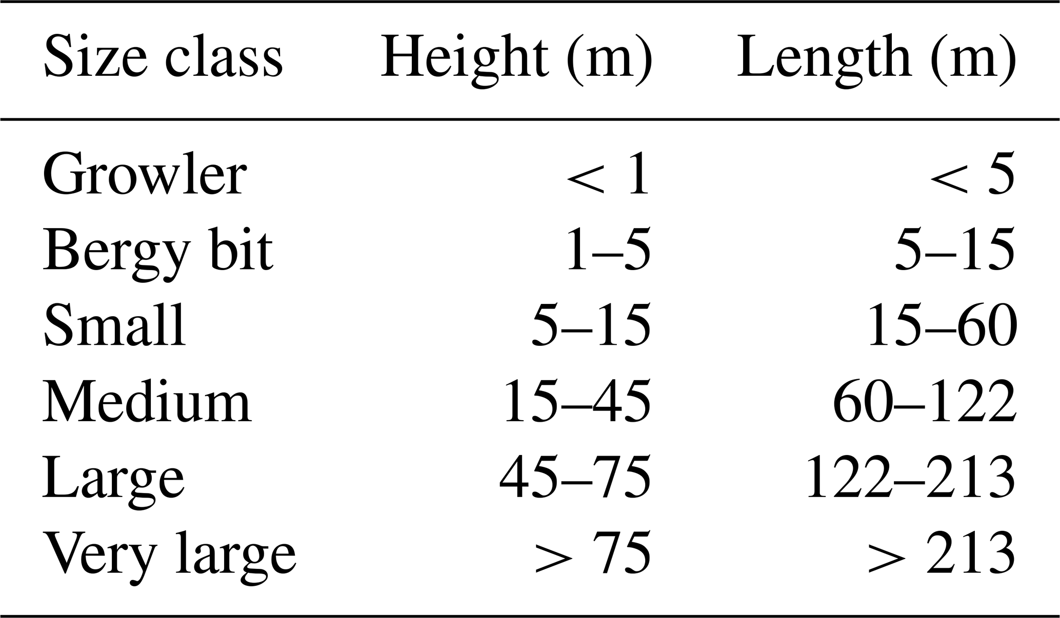
While icebergs are more common near ice–ocean boundaries, they drift across long distances with ocean currents and thus pose potential hazards even hundreds of kilometers away from any glacier (Schodlok et al., 2006). One such location is the western part of the North Atlantic Ocean, where icebergs are regularly transported south through the Davis Strait into high-traffic North Atlantic shipping lanes (Kollmeyer, 1978). Along this path, icebergs have been extensively surveyed (Jacka and Giles, 2007; Romanov et al., 2012) and are continuously tracked by the International Ice Patrol (IPP) (Murphy and Cass, 2012) according to size (Table 1) and shape (e.g., tabular vs. non-tabular). Despite the importance of these reports, they are limited in both temporal and spatial extent and are largely unavailable in polar regions. Remote-sensing techniques such as lidar (e.g., Scambos et al., 2005; Wagner et al., 2014; Stern et al., 2015; McGuire et al., 2016) and optical stereo photogrammetry (e.g., Enderlin and Hamilton, 2014; Sulak et al., 2017) have been used to evaluate both the vertical and horizontal extent of icebergs as tools with larger spatial coverage. However, microwave remote-sensing systems, such as radar altimeters (e.g., McIntyre and Cudlip, 1987; Tournadre et al., 2008, 2012, 2015) and scatterometers (e.g., Ballantyne and Long, 2002; Long et al., 2002; Aoki, 2003; Stuart and Long, 2011), are advantageous due to their independence from light and weather conditions.
Table 1Iceberg size classification defined by the International Ice Patrol.
Synthetic aperture radar (SAR) has shown to be a robust tool to detect smaller icebergs with a resolution down to the meter scale (e.g., Williams et al., 1999; Frost et al., 2016; Akbari and Brekke, 2018). SAR-based methods are typically based on intensity thresholds, based on the assumption that icebergs return a stronger backscatter signal than their surroundings (e.g., Willis et al., 1996; Silva and Bigg, 2005; Wesche and Dierking, 2012). More recently, object-based image analysis with a focus on classifying objects rather than individual pixels has also shown promise (Mazur et al., 2017). Techniques based on backscatter intensity alone, however, are suboptimal where the brightness between icebergs and background is similar; for example, when icebergs are surrounded by wind-roughened water (e.g., Willis et al., 1996; Wesche and Dierking, 2012). Such techniques can potentially be improved by polarimetric SAR (Howell et al., 2004; Denbina and Collins, 2012; Kim et al., 2012; Dierking and Wesche, 2014; Marino et al., 2016). However, standard SAR-based approaches provide information strictly pertaining to the horizontal extent and concentration of icebergs but do not provide information related to the height necessary to fully classify the icebergs according to Table 1.
The evaluation of height is not only necessary for classification, it is also crucial for assessing the three-dimensional surface morphology relevant to marine mammals (McNabb et al., 2016), the stability of the icebergs (Guttenberg et al., 2011), and expected keel depth (Enderlin et al., 2016). Moreover, iceberg morphology is related to the overall iceberg volume relevant to a number of important properties such as drift and decay (Hamley and Budd, 1986; Barker et al., 2004; Jacka and Giles, 2007; Crawford et al., 2018), freshwater contribution (Jacobs et al., 1992; Silva et al., 2006; Enderlin and Hamilton, 2014; Moon et al., 2018), and icebergs as a hazard (Bigg et al., 2018). The mass and thus mechanical properties (Romanov et al., 2012) and potential impact on structures and vessels (Liu et al., 2011) are also directly related to iceberg volume. The total volume of icebergs is difficult to estimate unless the subaerial (above water) morphology is measured. Here, the physical limitations of existing techniques in measuring morphology hamper consistent and accurate iceberg evaluation over large areas (Romanov et al., 2017). TanDEM-X SAR interferometry (InSAR) (Rosen et al., 2000) is a technique to extract topography from the phase information from two complex SAR scenes. This technique has previously been utilized to assess sea ice ridges (Dammann et al., 2017; Dierking et al., 2017; Yitayew et al., 2018). For icebergs, this technique was first demonstrated by García et al. (2012) and later validated using optical spaceborne photogrammetry data (Zakharov et al., 2017, 2019).
The work presented here expands upon prior work. First, we validate this technique using high-resolution airborne data from optical imagery in combination with and cross-validated by laser altimeters, resulting in ∼20 cm vertical accuracy. These missions were carefully planned with the German Aerospace Center for collocating TanDEM-X data acquisitions with both optical imagery and laser altimetry, forming comprehensive coordinated datasets. Second, we demonstrate possible applications and uses of this approach. We present and validate an alternate method to standard iceberg classification based on volume. Volume is arguably more relevant than standard measurements such as height and length for applications including freshwater contribution, drift, and potential impact on structures. We also investigate the derivation of possible iceberg keel depths relevant for grounding assessments and impact on subsea installations. Lastly, we include a discussion around necessary considerations including phase noise, signal penetration, and acquisition geometry. We also highlight potential limitations related to data availability, iceberg shape and size, and the impacts of drift.
2.1 TanDEM-X data and study area
This work utilizes data from TanDEM-X, an X-band SAR system that has been operating since 2010. Each individual satellite of the TanDEM-X constellation has a repeat-pass cycle of 11 d and an orbit design optimized for constellation flight, which allows simultaneous acquisitions between the two constellation partners. TanDEM-X is operated by the German Aerospace Center (DLR) and is currently the only system which can acquire SAR imagery with temporal lag on the order of milliseconds necessary to reliably and consistently evaluate topography of nonstationary surfaces undergoing slow motions. The system features two X-band SAR sensors, resulting in meter-scale resolution imagery.
This work utilizes a TanDEM-X bistatic acquisition from 29 November 2017 at 00:32:09.874 UTC over Buffer Island in Wordie Bay on the west side of the Antarctic Peninsula (Fig. 1). This is the region of the former Wordie Ice Shelf, which broke away from shore between 2008 and 2009. The region is often populated by numerous icebergs, ranging from a few meters to several hundred meters in width, frozen into the landfast sea ice as seen from an Operation IceBridge flight on 21 November 2017 (Fig. 2). The acquisition was taken in ascending orbit no. 58160 with an incident angle of 38.5∘. The acquisition features two dual polarization horizontal and vertical (HH and VV) strip-map images with a swath width of 15 km and a time lag of 10 ms. The perpendicular and along-track baseline between images was 154 and 151 m, respectively.

Figure 1Study area situated around Buffer Island in Wordie Bay, Antarctica.
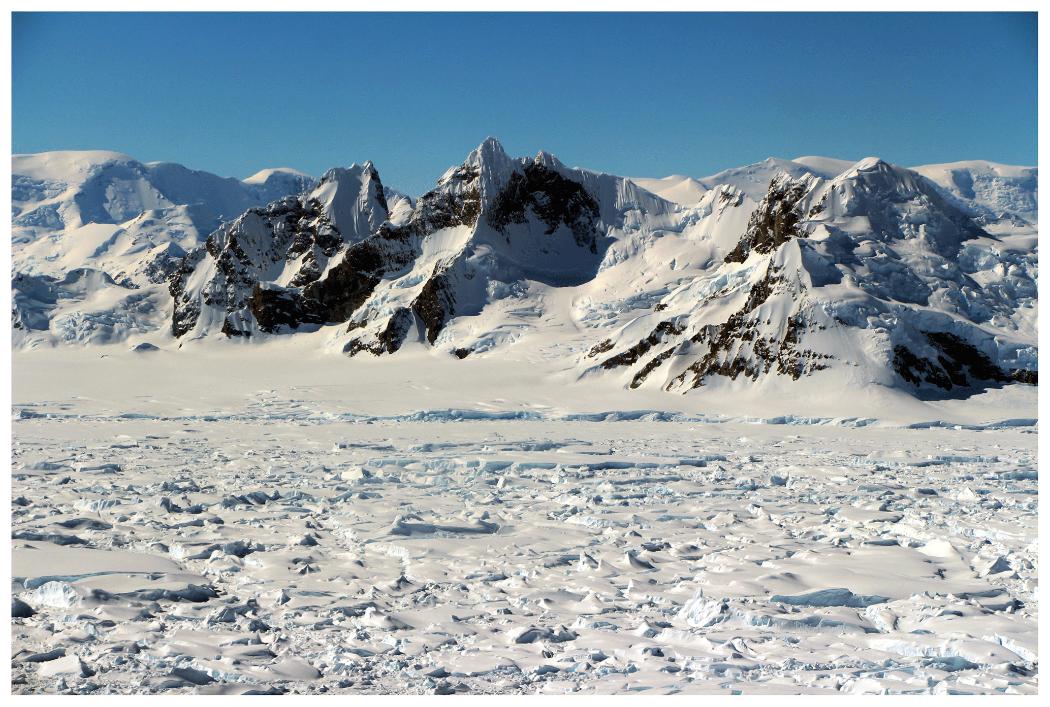
Figure 2Photograph of Wordie Bay on 21 November 2017 taken at 69.230∘ S and 68.430∘ W. The broken-up remains of the Wordie Ice Shelf are in the foreground. Photo credit: John Sonntag.
2.2 Interferometric SAR processing
InSAR is a technique utilizing two complex SAR scenes, where the resulting interferogram represents the phase difference, ΔΦ, between the two scenes and is represented by phase values in the range [−π, π). For TanDEM-X data with large spatial and short temporal baselines, the observed values for ΔΦ are largely attributed to the phase component due to topography ΔΦtopo:
where R is the slant range, B⊥ is the perpendicular baseline, θ is the incident angle, λ is the wavelength, and h is the topographic height. If the height exceeds a certain threshold called the height of ambiguity, the phase will wrap around from −π to π causing phase ambiguities. The height of ambiguity can be expressed as follows:
For the image used here, the height of ambiguity is ha= 41.8 m.
We processed the VV channel of the complex TanDEM-X (λ=3.1 cm) scene for backscatter intensity and phase-derived height using the GAMMA Software (Werner et al., 2000). For backscatter, this involved multilooking of 2×2 pixels (resulting in resolution of roughly 2.7 m in range and 4.7 m in azimuth) and filtering 5×5 pixels using a standard boxcar filter. To obtain phase-derived height (referred to hereafter as the InSAR Digital Elevation Model or InSAR DEM), we followed a standard InSAR processing workflow (Rosen et al., 2000). This processes involves multilooking (2×2 pixels) and adaptive phase filtering (Goldstein and Werner, 1998) to reduce phase noise. Here, we used a relatively small fast Fourier transform (FFT) filtering window size of 8. The small window was chosen to preserve as much detail of the icebergs as possible. Finally, we geocoded the backscatter image and interferogram in a universal transverse Mercator (UTM) 17S projection (with a WGS84 datum in an ellipsoidal reference height system) and resampled to a 2.5 m square pixel spacing.
The theoretical relative height accuracy of the InSAR DEM can be calculated as follows:
where σϕ is the standard deviation of the InSAR phase estimate, which is expressed as follows:
in which NL is the independent number of looks and γ is the interferometric coherence (Rosen et al., 2000; Dierking et al., 2017). Based on an average coherence, γ∼0.7 for our study area, this results in a relative height accuracy, σh∼2.5 m.
2.3 Iceberg classification
We discriminated icebergs from surrounding ice by applying the InSAR DEM. Our method requires a minimum iceberg height of 5 m, twice that of the height accuracy σh, which means we cannot detect growlers and bergy bits (Table 1). Setting such a high threshold results in minimized false positives from phase noise. Once an initial iceberg mask was created via thresholding, we performed a subsequent geometric-opening operation to remove noise in the initial mask by removing objects of less than roughly 10×10 pixels in size.
We classified the delineated icebergs in multiple ways. First, we use the classification outlined in Table 1: small, medium, large, and extra-large according to equivalent length (square root of total area) and height. Second, we classified them as tabular or non-tabular through the ratio of height above water to equivalent length because tabular icebergs have a smaller height compared to their length. Tabular icebergs are those that calve from floating ice shelves or tongues that are rectangular cuboid shape and of stable geometry such that they do not flip from their original orientation. Because of the nature of their formation, tabular icebergs are typically “medium” height (Table 1) but “extra-large” length, as the stability for their shape requires a minimum length of approximately 5 times the height (Bass, 1980). A tabular iceberg classification is important as it both impacts the predicted keel depth and provides information on the iceberg source location (tabular icebergs are created from floating termini and ice shelves). Tabular icebergs eventually decay through melt and fracture into shapes belonging to the non-tabular category.
Third, we calculate the iceberg volume. The iceberg subaerial volume (volume above sea level) can be calculated by integrating the phase-derived height above a reference surface within the delineated areas occupied by icebergs. Integration steps equal the pixel spacing of 2.5 m. The total iceberg volume then can be inferred from subaerial volume, which is 11% of the total volume based on an assumed density for ice and sea water of 917 and 1030 kg m−3, respectively. And finally, based on physics of floating objects, we calculate the limits of minimum and maximum keel depths (draft, d) based on volume (V), waterline area (A), and length (L) using idealized shapes and stability analyses (e.g., Bass, 1980). We define a physics-based minimum keel depth as that for tabular icebergs , assuming a rectangular cuboid. We specifically define extreme maximum keel depth (again based on physics of idealized shapes) as an inverted pyramid or cone ; however, this shape is unlikely to persist due to rapid melting of a pointed keel. Given this definition of maximum keel depth as the upper limit, we note that the window of real-world keel depths is certainly smaller. We also, therefore, estimate “expected” keel depth of d=2.91L0.71, where L is the waterline length of the iceberg in meters. This approach is suggested by Barker et al. (2004) based on physics combined with limited measurements. A similar analyses was performed by Sulak et al. (2017).
2.4 Validation data
The TanDEM-X data over Wordie Bay were acquired in conjunction with the Operation IceBridge (OIB) fall 2017 Antarctic campaign on 21 November 2017, of which the OIB/TanDEM-X Antarctic Science Campaign (OTASC) (Nghiem et al., 2018) was a component. Recognizing the potential value of OTASC for operational sea ice and iceberg applications, the U.S. National Ice Center participated, supported, and contributed to the success of OTASC (Nghiem et al., 2018). OIB is a decade-long series of annual Arctic and Antarctic airborne surveys intended to bridge the gap between polar land and sea ice measurements collected by NASA's ICESat-1 and ICESat-2 spacecraft (Zwally et al., 2002; Markus et al., 2017). The aircraft used for the 2017 Antarctic campaign was NASA's P-3 Orion, a long-range, four-engine turboprop capable of flights of up to 10 h in length, at low altitude, and at speeds of 250 knots. For this campaign the aircraft was based in distant Ushuaia, Argentina, owing to the lack of suitable air basing facilities for such a large aircraft on the Antarctic continent. This arrangement limited the on-site survey time available.
For the OTASC-coordinated flights, OIB selected suitable TanDEM-X ground tracks for the day of each flight and coordinated the aircraft's arrival on the track to be as close in time to that of the spacecraft as practical. The aircraft was equipped with a suite of geophysical instruments, including a pair of scanning laser altimeters, known as the Airborne Topographic Mapper, or ATM (Martin et al., 2012), a digital high-resolution camera system called the Digital Mapping System (DMS) (Dominguez, 2010), and associated GPS, inertial, and precise navigation systems. When merged, the three-dimensional point cloud data from the ATM and the geolocated imagery from the DMS enabled the construction of a 250 m wide, submeter resolution digital elevation model (DEM) with a vertical accuracy of ∼0.2 m and 10 cm×10 cm pixel spacing (Nghiem et al., 2018). Data were acquired over our study area in Wordie Bay on 21 November, 2017 (17:26:58–17:28:34 UTC) with acquisition ID 172759 (Studinger, 2016), 8 d prior to the TanDEM-X acquisition. No significant motion took place between the two datasets. The icebergs were confirmed stationary, frozen into the landfast ice, by consecutive TanDEM-X overpasses. The data were re-projected from WGS84 polar stereographic to WGS84 UTM 17S, equal to that of the geocoded SAR data and resampled to a 0.5 m square pixel spacing. The model is referred to from here on as DMS DEM.
We utilized a roughly 15 km×15 km section of the TanDEM-X acquisition centered around Buffer Island. We processed the scene for backscatter intensity (Fig. 3a) and phase-derived height (InSAR DEM) (Fig. 3b). These data exhibit large amounts of stationary icebergs of different sizes enclosed by landfast sea ice. We compared the TanDEM-X backscatter and InSAR DEM with the DMS DEM. This comparison was done within a small, roughly 10 km2 subset (red rectangle in Fig. 3) around the validation data (Fig. 4a and b). The DMS DEM dataset follows a curved path covering many small icebergs and parts of some larger icebergs (Fig. 4c). For validation, we defined four transects (T1 to T4) and six areas (A1 to A6) completely situated within the boundaries of the DMS DEM. These are spread throughout the dataset and cover different icebergs and iceberg sizes.
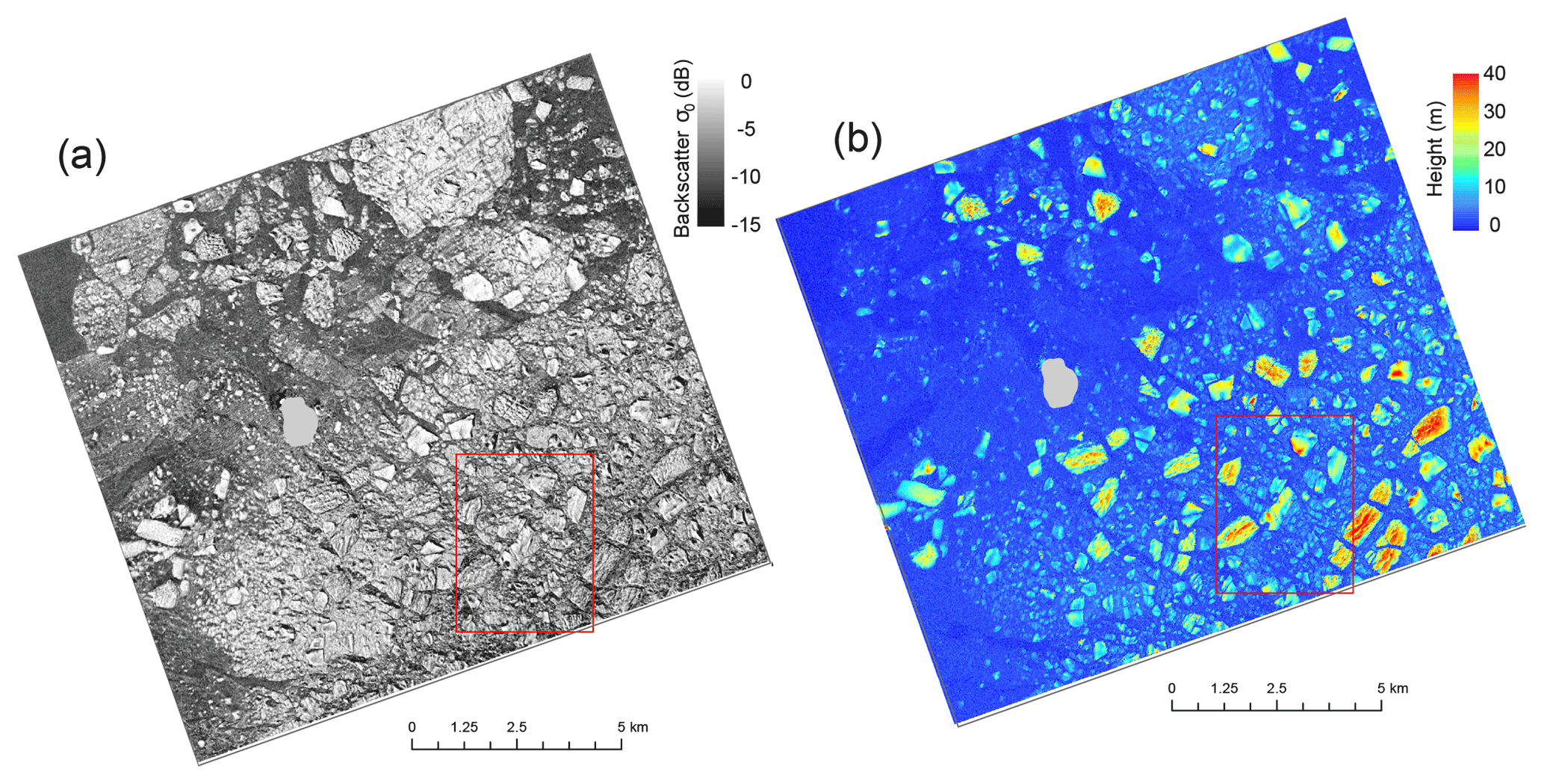
Figure 3Cropped area of the TanDEM-X scene processed for backscatter intensity (a) and interferometric height (InSAR DEM) (b). The red rectangle signifies validation area. Buffer Island is masked out in light gray.
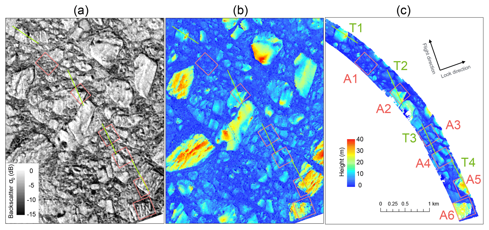
Figure 4Backscatter (a) and InSAR DEM (b) over the validation area. Panel (c) is the validation DEM (DMS DEM). Red rectangles signify individual validation areas. Green lines signify validation cross sections.

Figure 5Comparison of interferometric height (InSAR DEM) (blue), backscatter (black), and OIB DEM (DMS DEM) (red) along transects. Dashed circles indicate locations of significant discrepancy between DEMs, either where DMS DEM > InSAR DEM (turquoise) or DMS DEM < InSAR DEM (green). Purple arrows indicate sections of significant (>10 m) variability in the InSAR DEM not present in the DMS DEM.
Transects T1, T2, and T4 cross larger icebergs with heights exceeding 20 m, while T3 crosses smaller icebergs with heights below 10 m. For all transects, the DMS DEM compares reasonably well with the InSAR DEM, as they generally follow the meter-scale topography (Fig. 5). However, there are several outliers along the transects resulting in an average root-mean-square error (RMSE) of 3.46 m (ranging between 4.64 m for T1 and 2.23 m for T3). First, the DMS DEM is smoother than the InSAR DEM, most likely due to (1) phase noise equivalent to σh∼2.5 m and (2) substantial averaging of the DMS DEM product from its original pixel spacing. Second, there are discrepancies between the InSAR DEM and DMS DEM at the location of rapid elevation changes with vertical or steep slopes (see circled areas in Fig. 5). This discrepancy is likely due to layover (compression of targets closest to the satellite) effects, increasing elevation in the InSAR DEM on the side of the iceberg facing the satellite and vice versa. Third, two areas feature substantial variability of over 10 m in the InSAR DEM not represented in the DMS DEM (see purple arrows in Fig. 5). These areas correspond to low backscatter (see black lines in Fig. 5), likely as a result of radar shadowing. The low backscatter can significantly reduce coherence through low signal-to-noise ratios and thus height accuracy according to Eq. (4).
The backscatter profiles shown in Fig. 5 exhibit variability that is somewhat correlated with the location of icebergs (i.e., areas of sea ice in between icebergs corresponds to reduced backscatter and icebergs correspond to relatively high backscatter), which has been observed before (Willis et al., 1996; Silva and Bigg, 2005; Wesche and Dierking, 2012). However, there is not a direct relationship between backscatter and iceberg elevation in our dataset. We quantified the low correlation between the two in our data by estimating correlation coefficient between backscatter and DMS DEM for areas A1 to A6 (not shown). These low correlations (mean R=0.58) are expected because surface roughness and slope dominate radar brightness, rather than the elevation of icebergs. Backscatter is therefore not sufficient to infer either iceberg height or volumetric size.
We similarly compared the DMS DEM and InSAR DEM for areas A1 to A6 (Fig. 6) and show higher correlations between the DMS DEM and InSAR DEM (mean R=0.69) than the DMS DEM and backscatter. The datasets show a close to 1 : 1 linear trend with R values exceeding 0.6. However, there are substantial outliers for the reasons pointed out previously, leading to RMSE values ranging between 1.89 m (A1) and 7.08 m (A5). To further the understanding of these outliers, we calculated the differences between the DMS DEM and the InSAR DEM. We examined the most significant differences near A3 to A6 (see Fig. 7). These differences indicate that substantial offsets are located around steep vertical sides of icebergs (see circled area in Fig. 7 and circles in Fig. 5). This cannot be attributed to phase unwrapping errors as offsets typically do not exceed ha. They are also not likely to be attributed to an offset between DEMs, as such offsets are not systematically occurring in similar locations. As the offset occurs in a region of low backscatter values, reduced coherence is the most likely source of the observed differences. Despite the inaccuracies in areas of low backscatter, the InSAR DEM compares well with the DMS DEM, indicating that the InSAR DEM sufficiently captures the surface morphology of icebergs and enables the derivation of iceberg volume.
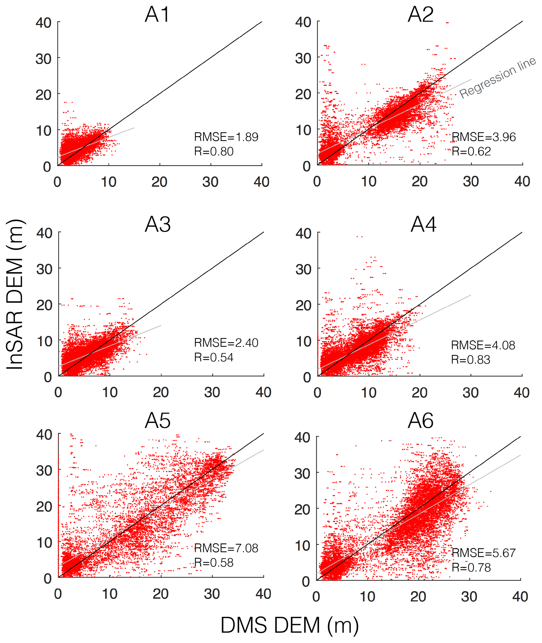
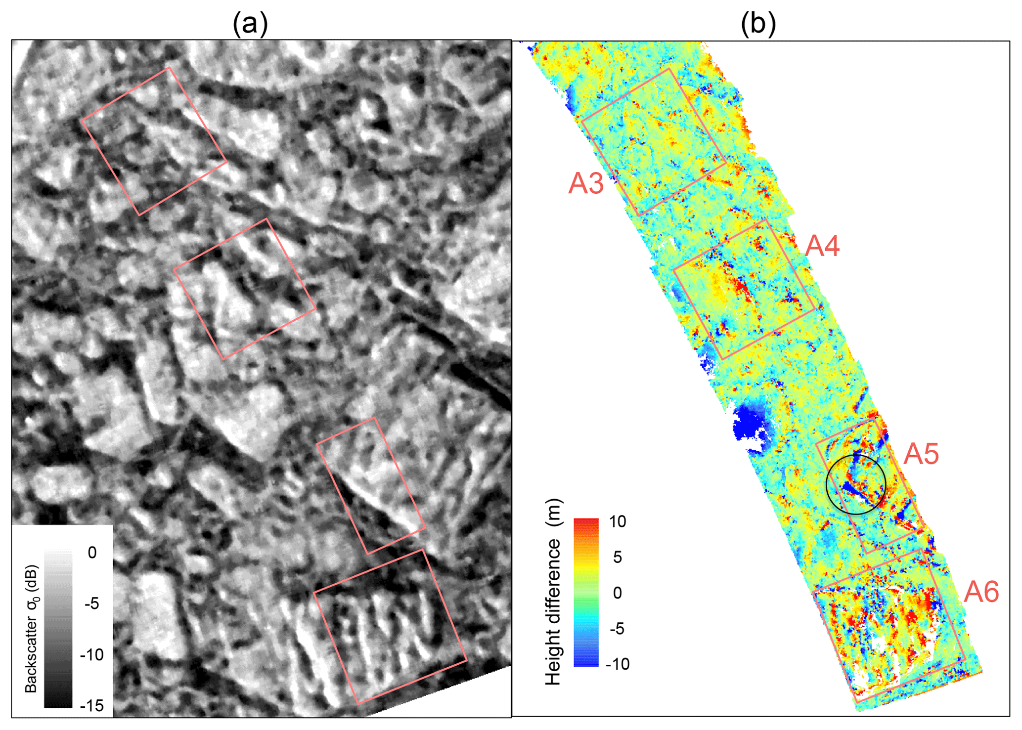
Figure 7(a) Intensity cropped around four validation areas. Panel (b) is the height difference (InSAR DEM – DMS DEM). The black circle indicates area of substantial difference between the DEMs.
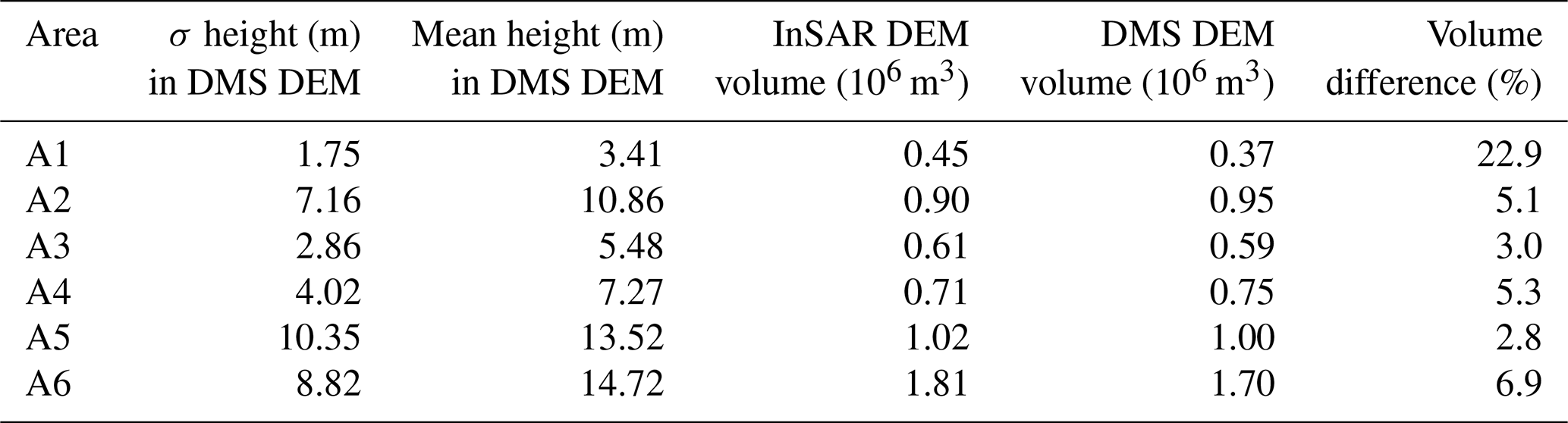
We calculated the total volume of ice above a reference surface (i.e., zero elevation calibrated to the lowest InSAR DEM values; see the left corner of Fig. 3b) for A1 to A6. The total volumes calculated from the DMS DEM and InSAR DEM for each area are listed in Table 2. The iceberg sizes enclosed by the boundary of areas A1 to A6 vary greatly, from having meter-scale relief to several tens of meters, and thus greatly vary in total iceberg volume and relative volume accuracy. For instance, A1 contains the lowest volume of icebergs but features the largest discrepancy (measured in %) between the DEMs. The largest iceberg in terms of height is found in A5, which has the best match between the DEMs. These results indicate that volume is not captured well for small icebergs such as growlers and bergy bits and that volume estimates are in general most accurate for larger icebergs. However, comparing A2 and A3 reveals exceptions from a direct relationship between height and accuracy.
4.1 Volume classification
We demonstrate here the advantages of using TanDEM-X for evaluating icebergs using InSAR. We show that TanDEM-X data enable assessment of subaerial morphology and volume of icebergs with meter-scale resolution in a cost-effective manner in comparison with air reconnaissance. We found that InSAR-derived volumes agree with estimated volumes based on the Operation IceBridge data within 7 %, except for icebergs with a small topographic relief ranging from a few centimeters to meters (barely visible in the interferometric phase), where the volumetric difference was found to be 23 %. InSAR-based iceberg assessments can thus potentially be used to enhance understanding of the evolution of icebergs and their impact on local ecosystems. SAR signals do not rely on daylight or weather conditions. Hence InSAR-derived measurements could also potentially be used in an operational setting for tactical decision-making.
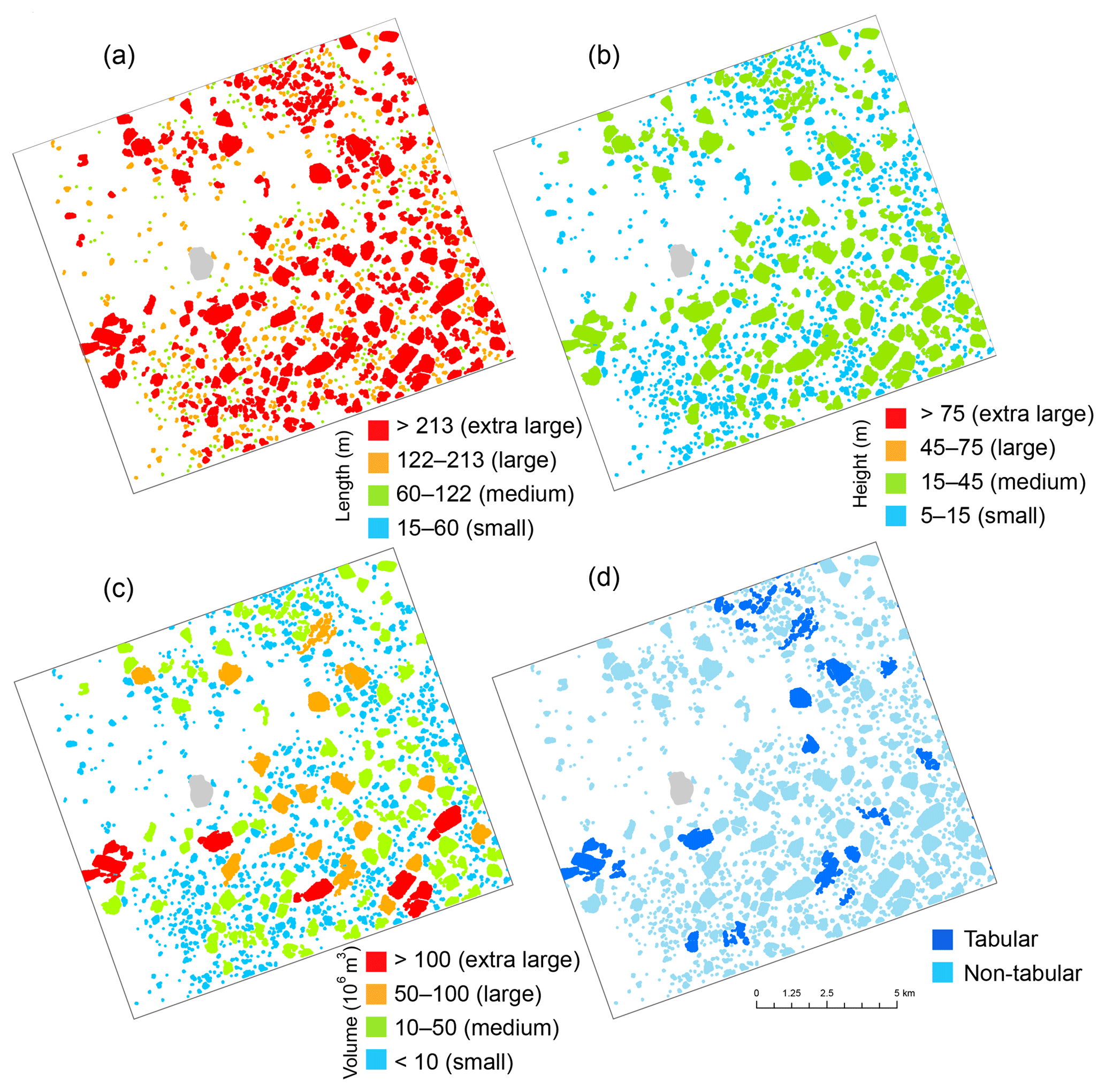
Figure 8Iceberg classification based on length scale (a), maximum height (b), volume (c), and tabular height-to-length threshold (d). Buffer Island is masked out in light gray.
We furthermore explored the potential for classifying icebergs according to volume and how such classification differs from standard approaches. We initially classified icebergs using the InSAR DEM according to the International Ice Patrol (IIP) thresholds (Table 1). This results in classification of small, medium, large, and extra-large icebergs. However, with this classification method, only medium, large, and extra-large icebergs are present in our study area based on equivalent length (Fig. 8a) and only small and medium icebergs based on height (Fig. 8b). Here, icebergs that we classify as extra-large in Fig. 8a are medium according to Fig. 8b. One likely explanation for this difference is that iceberg shape varies greatly between the region surveyed by IIP near the Grand Banks, Newfoundland, and our study region in Antarctica dominated by tabular icebergs. This suggests that a one-dimensional metric is suboptimal to describe icebergs.
We classified icebergs according to their derived total volume (Fig. 8c). The classification thresholds were chosen with close to equal volumetric bin sizes of about 50×106 m3, with the exception of the smallest icebergs, enabling an incorporation of all icebergs in our study region into four classes. In general, larger icebergs in terms of surface area (Fig. 8a) are also classified as larger in terms of volume (Fig. 8c) and vice versa. This is expected since iceberg height is limited by its horizontal extent to remain stable and not flip over on its side. Tabular icebergs have larger volumes relative to their height than their non-tabular counterparts. Fig. 8d shows the distribution of tabular icebergs in our study area, identified according to a length-to-height ratio of 5. The value of our proposed volumetric classification scheme is its application in areas where iceberg volume or mass is of direct relevance to important properties and processes. In a final alternative approach, we classified icebergs according to physics-based minimum and maximum keel depths as well as an estimate based on past data (Fig. 9). This type of classification has relevance for iceberg interactions with the sea floor, such as grounding and impacts on subsea installations.
4.2 Method constraints
Even with its potential advantages, TanDEM-X has limitations for the task of iceberg detection and classification due to low data availability over ice-covered waters in particular. The 11 d repeat-pass cycle is also a disadvantage as it reduces the potential of TanDEM-X for monitoring of icebergs with significant drift speeds. Even so, volume evaluation using TanDEM-X has a synergistic potential for complementing existing products. For instance, a single InSAR pair from this mission could be used to identify icebergs and estimate their size and volume. The icebergs could then be tracked through time using other SAR systems, such as Sentinel-1, improving temporal coverage. The accuracy of TanDEM-X in deriving iceberg height critically depends on the perpendicular baseline (Eq. 3), which may be suboptimal depending on location and time. The primary goal of the TanDEM-X mission and ongoing operations is to acquire a DEM over land. Therefore, baselines and the resulting height of ambiguities may not be optimal over polar oceans for evaluation of icebergs. This was the case for the OTASC campaign, where the height of ambiguities ranged between 40 and 50 m (∼150 m perpendicular baseline), making it difficult to evaluate growlers with a subaerial vertical extent of less than 1 m. A height of ambiguity of less than 10 m would have been preferred for this application but was only possible during the TanDEM-X Science Phase in 2015 (Dammann et al., 2017; Dierking et al., 2017).
Beyond the constraints related to TanDEM-X data, there can be inherent environmental limitations impacting the interferometric processing and analysis. Examples are situations where icebergs are in a state of drift or situations where significant penetration of the SAR signal into the freshwater ice occurs. Atmospheric effects, coregistration errors, and phase changes due to surface change or deformation can also theoretically result in a phase uncertainty but are unlikely to be significant for bistatic acquisitions. The interferometric phase, ΔΦ, is sensitive not only to topography but also surface motion. Displacement in line-of-sight direction (ΔrLOS) results in a phase change according to (Dammann et al., 2016). Ice drift can potentially reach close to 1 m s−1, which for bistatic mode with a 10 ms temporal baseline can result in a phase change ΔΦdisp∼4 radians. With a height of ambiguity of tens of meters, the phase contribution from motion is significant but can potentially be removed. For instance, if the iceberg is surrounded by drifting sea ice, the icebergs may possibly drift at comparable speeds if frozen within the sea ice. If not frozen in, the icebergs may drift with different speeds than surrounding sea ice, including the possibility of drift in the opposite direction if deeper currents drive iceberg drift. In such a case, the phase of the surrounding sea ice can be used to calibrate roughly zero elevation independent of speed. In the absence of sea ice or in the case of non-homogenous drift, the outer perimeter of the iceberg can also sometimes be used for calibration. This is, however, difficult if the sides of the iceberg are steep.
When comparing phase-derived height from TanDEM-X with the validation dataset, it is necessary to consider possible significant horizontal or vertical mismatch between the datasets. In this work we strictly geocoded the TanDEM-X data based on orbit position. A difference in geoid correction between the datasets can lead to a translational lateral mismatch of up to 80 m, hence we shifted the DMS DEM 67 m to visually match the InSAR DEM. Based on the strong backscatter gradients of the iceberg edges, a meter-scale accuracy could be ensured. We also calibrated the height of both datasets to zero height in an area of no icebergs. We did not perform an absolute height calibration, which inevitably results in remaining inaccuracies, such as spatial translational and rotational offsets. Such small positioning offsets of the InSAR DEM might cause large (>10 m) height offsets near the edges of icebergs, possibly contributing to the offsets seen in Fig. 7. Spatial offsets can be reduced by the use of external control points from IceSat or tie points of neighboring TanDEM-X tracks to improve the InSAR DEM referencing.
It is necessary to consider possible penetration of the X-band SAR signal. Both laser altimetry (ATM) and optical photogrammetry (DMS) generally result in a DEM of the ice or snow surface. On the other hand, ice topography as derived using InSAR is not necessarily the topography of the ice surface but rather reflects the elevation of the interferometric phase center (Rignot et al., 2001). SAR signals may significantly penetrate into the ice and reflect off subsurface layers or impurities (e.g., air bubbles, fractures) within an iceberg. Little is known about the exact penetration depth of X-band SAR, but it decreases with rising temperature and water content (Gardelle et al., 2012; Hall and Martinec, 1985). TanDEM-X was shown to penetrate up to 7 m into firn and glacier ice (Dehecq et al., 2016). In Antarctica, Davis and Poznyak (1993) measured penetration depths at 10 GHz reaching between 2.1 and 4.7 m, and Surdyk (2002) reported a 4 m penetration depth at 10.7 GHz into ice at −88 ∘C (Gardelle et al., 2012). The penetration of X-band SAR into icebergs may be substantially lower as icebergs are subjected to saline water, warmer surfaces and internal temperatures close to those of the surrounding water, and contain limited fern, which significantly impacts penetration in glacier studies. For exposed ice during warmer parts of the year, Rignot et al. (2001) reported no significant penetration (±1–2 m) for exposed ice near Jakobshavn Glacier, Greenland. At the time of the acquisition used here, the temperature at the San Martín Base, approximately 110 km north-northwest of Buffer Island (Fig. 1), was roughly +2 ∘C and remained above freezing for the prior 12 h. The resulting X-band penetration depth based on the warm ice and snow surfaces is, therefore, likely insignificant.
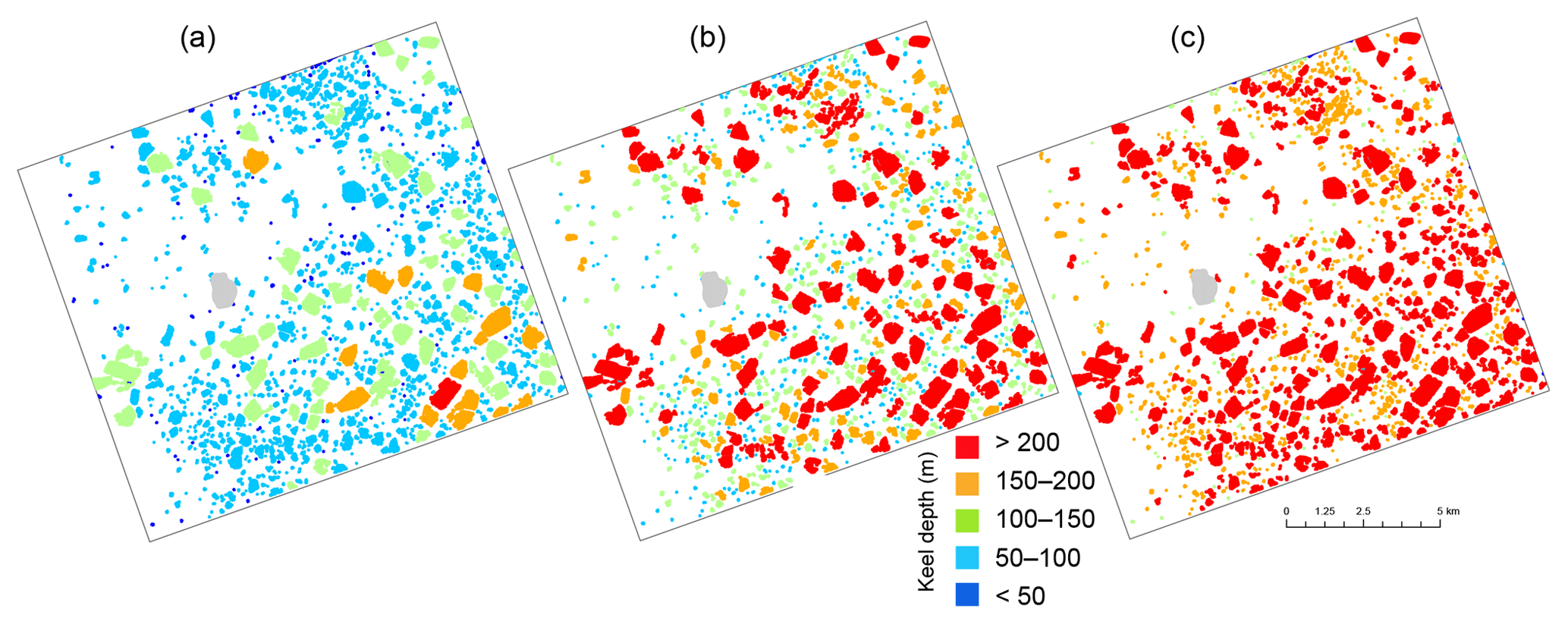
The classification methods described here are associated with limitations. It has proven difficult in this work to classify bergy bits and growlers based on their modest subaerial relief. For the small to extra-large icebergs that can be classified, the derived volume is based on assumptions that the icebergs are in hydrostatic equilibrium. Close to the coast, as is the case here, it will be necessary to assess bathymetric data to assess the validity of that assumption based on phase-derived height, an approximate sail-to-keel ratio, and bathymetric information. We estimated approximate keel depths based on derived iceberg volume and assumed hydrostatic equilibrium (Fig. 9). For the extra-large icebergs in this work, the difference between the estimated minimum and maximum keel depths can reach upwards of 100 m. This can make it problematic to determine whether icebergs are floating or grounded in locations where bathymetric depth falls within this window. Also, keel depth estimates are based on the volume or equivalent length of the iceberg. If two icebergs are connected underwater, then keel depths can be larger than would be calculated by treating the two subaerial parts as individual icebergs. While such a situation may not critically impact estimates of, for example, potential freshwater contribution of icebergs, they could lead to significant errors of estimated keel depth, iceberg drift and decay, and their hazard potential for maritime installations.
In this work, we applied bistatic InSAR data from the TanDEM-X mission over Wordie Bay, Antarctica, to derive topography and volume information of icebergs. We initially validated the phase-derived height of icebergs with elevation data acquired from the OIB/TanDEM-X Antarctic Science Campaign (OTASC). This validation demonstrates that bistatic interferometry can be a valuable tool in assessing iceberg morphology and volume. We furthermore classified icebergs based on volume. Iceberg volume incorporates both the height dimension and the length scale and is likely an advantageous metric for a number of applications. For instance, volume is of key relevance not only to offshore operations and ice management but also in the context of marine habitat and ecosystem mapping and glaciology research. Based on derived volume, we were able to estimate the tabular nature of icebergs and bracket minimum and maximum keel depths, resulting in a range of bathymetric depths where the surveyed icebergs can potentially interact with the sea floor. A detailed discussion of the main uncertainties affecting these estimates was provided. Further work is needed to investigate how to most effectively and accurately classify icebergs using InSAR for different applications.
TanDEM-X is the only current spaceborne SAR system that can be used to consistently evaluate the morphology and volume of icebergs. TanDEM-X has a relatively narrow achievable swath width in strip-map mode (∼30 km for single polarization and ∼15 km for dual polarization), which is suboptimal for iceberg monitoring across large spatial scales. Future systems with a high-resolution wide swath mode may be able to overcome this limitation. TanDEM-X has a repeat-pass cycle of 11 d, limiting data availability and reducing the applicability of InSAR in an operational setting. Future systems such as the LOTUSat-1 (2021 launch) and LOTUSat-2 (2025) X-band SAR missions (Pham, 2017) may alleviate this concern. However, the capability of LOTUSat for iceberg detection needs to be evaluated specifically based on LOTUSat SAR characteristics and orbit configurations. The planned TanDEM-L mission (Moreira et al., 2015) may further contribute synergistic data in time and space; however, it is unclear how L-band SAR would differ from X-band in assessing iceberg volume due to larger penetration depth. Although the data availability of TanDEM-X is suboptimal for effective ice management and support of operations, volume products could still be a great asset in conjunction with other SAR systems. We also argue that TanDEM-X has the potential to be a valuable tool for deriving morphological statistics of icebergs to complement volume estimates by other observation methods. Such statistics could provide value for calving estimates, iceberg drift modeling, and habitat mapping.
TanDEM-X data from this analysis can be obtained from the German Aerospace Center (DLR) and downloaded from the Earth Observation on the Web (EOWEB; https://eoweb.dlr.de, last access: 23 March 2019) portal. Data from the Operation IceBridge mission can be accessed at the National Snow and Ice Data Center (NSIDC; https://nsidc.org/data/icebridge, last access: 23 March 2019), which is a Distributed Active Archive Center (DAAC).
DOD conducted the interferometric processing and analysis and drafted the initial manuscript. LEBE and SVN provided critical guidance on all aspects of the analysis and manuscript. SVN, NTK, JGS, and TB contributed to the thorough planning and successful execution of the OIB/TanDEM-X Antarctic Science Campaign, providing satellite and aircraft data used in this research. EP provided valuable expertise relevant to icebergs and iceberg classification. FJM and ARM contributed guidance in terms of interferometric analysis and interpretation. All co-authors also provided valuable recommendations and corrections resulting in the final paper.
The authors declare that they have no conflict of interest.
TanDEM-X data were provided free of charge by the DLR through science proposals XTI_GLAC6921 and XTI_GLAC7297. Operation IceBridge data were provided by NASA. The research carried out at the Jet Propulsion Laboratory (Son V. Nghiem), California Institute of Technology, was supported by the NASA Cryosphere Science Program and in part by the NASA Earth Science R&A Program.
This research has been supported by the Swedish National Space Agency (grant no. 192/15) and StormGeo.
This paper was edited by John Yackel and reviewed by three anonymous referees.
Akbari, V. and Brekke, C.: Iceberg detection in open and ice-infested waters using C-band polarimetric synthetic aperture radar, IEEE T. Geosci. Remote, 56, 407–421, 2018.
Aoki, S.: Seasonal and spatial variations of iceberg drift off Dronning Maud Land, Antarctica, detected by satellite scatterometers, J. Oceanogr., 59, 629–635, 2003.
Arrigo, K. R. and van Dijken, G. L.: Impact of iceberg C-19 on Ross Sea primary production, Geophys. Res. Lett., 30, 1836, https://doi.org/10.1029/2003GL017721, 2003.
Ballantyne, J. and Long, D. G.: A multidecadal study of the number of Antarctic icebergs using scatterometer data, IEEE International Geoscience and Remote Sensing Symposium, 24–28 June 2002, Toronto, Ontario, Canada, 5, 3029–3031, 2002.
Barker, A., Sayed, M., and Carrieres, T.: Determination of iceberg draft, mass and cross-sectional areas, The fourteenth international offshore and polar engineering conference, 23–28 May 2004, Toulon, France, 2004.
Bass, D.: Stability of icebergs, Ann. Glaciol., 1, 43–47, https://doi.org/10.3189/S0260305500016943, 1980.
Bigg, G. R., Cropper, T., O'Neill, C. K., Arnold, A. K., Fleming, A. H., Marsh, R., Ivchenko, V., Fournier, N., Osborne, M., and Stephens, R.: A model for assessing iceberg hazard, Nat. Hazards, 92, 1113–1136, https://doi.org/10.1007/s11069-018-3243-x, 2018.
Blundell, G. M., Womble, J. N., Pendleton, G. W., Karpovich, S. A., Gende, S. M., and Herreman, J. K.: Use of glacial and terrestrial habitats by harbor seals in Glacier Bay, Alaska: costs and benefits, Mar. Ecol. Prog. Ser., 429, 277–290, https://doi.org/10.3354/meps09073, 2011.
Crawford, A. J., Mueller, D., and Joyal, G.: Surveying Drifting Icebergs and Ice Islands: Deterioration Detection and Mass Estimation with Aerial Photogrammetry and Laser Scanning, Remote Sens., 10, 575, https://doi.org/10.3390/rs10040575, 2018.
Dammann, D. O., Eicken, H., Meyer, F., and Mahoney, A.: Assessing small-scale deformation and stability of landfast sea ice on seasonal timescales through L-band SAR interferometry and inverse modeling, Remote Sens. Environ., 187, 492–504, https://doi.org/10.1016/j.rse.2016.10.032, 2016.
Dammann, D. O., Eicken, H., Saiet, E., Mahoney, A., Meyer, F., and George, J. C.: Traversing sea ice – linking surface roughness and ice trafficability through SAR polarimetry and interferometry, IEEE J. Sel. Top. Appl., 11, 416–433, https://doi.org/10.1109/JSTARS.2017.2764961, 2017.
Davis, C. H. and Poznyak, V. I.: The depth of penetration in Antarctic firn at 10 GHz, IEEE T. Geosci. Remote, 31, 1107–1111, https://doi.org/10.1109/36.263784, 1993.
Dehecq, A., Millan, R., Berthier, E., Gourmelen, N., Trouvé, E., and Vionnet, V.: Elevation Changes Inferred From TanDEM-X Data Over the Mont-Blanc Area: Impact of the X-Band Interferometric Bias, IEEE J. Sel. Top. Appl., 9, 3870–3882, https://doi.org/10.1109/JSTARS.2016.2581482, 2016.
Denbina, M. and Collins, M. J.: Iceberg detection using compact polarimetric synthetic aperture radar, Atmos.-Ocean, 50, 437–446, 2012.
Dierking, W. and Wesche, C.: C-Band radar polarimetry – useful for detection of icebergs in sea ice?, IEEE T. Geosci. Remote, 52, 25–37, https://doi.org/10.1109/TGRS.2012.2234756, 2014.
Dierking, W., Lang, O., and Busche, T.: Sea ice local surface topography from single-pass satellite InSAR measurements: a feasibility study, The Cryosphere, 11, 1967–1985, https://doi.org/10.5194/tc-11-1967-2017, 2017.
Dominguez, R.: IceBridge DMS L1B Geolocated and Orthorectified Images, version 1, NASA DAAC at the National Snow and Ice Data Center, Boulder, Colorado USA, 2010 (updated 2013).
Eik, K. and Gudmestad, O. T.: Iceberg management and impact on design of offshore structures, Cold Reg. Sci. Technol., 63, 15–28, https://doi.org/10.1016/j.coldregions.2010.04.008, 2010.
Enderlin, E. and Hamilton, G.: Estimates of iceberg submarine melting from high-resolution digital elevation models: application to Sermilik Fjord, East Greenland, J. Glaciol., 60, 1084–1092, https://doi.org/10.3189/2014JoG14J085, 2014.
Enderlin, E. M., Hamilton, G. S., Straneo, F., and Sutherland, D. A.: Iceberg meltwater fluxes dominate the freshwater budget in Greenland's iceberg-congested glacial fjords, Geophys. Res. Lett., 43, 11287–11294, 2016.
Frost, A., Ressel, R., and Lehner, S.: Automated iceberg detection using high-resolution X-band SAR images, Can. J. Remote Sens., 42, 354–366, 2016.
García, J. A., Eyssartier, K., López-Dekker, P., Prats, P., De Zan, F., Krieger, G., and Busche, T.: Monitoring the Petermann ice island with TanDEM-X, Geoscience and Remote Sensing Symposium (IGARSS), 22–27 July 2012, Munich, Germany, 2012 IEEE International, 1912–1915, 2012.
Gardelle, J., Berthier, E., and Arnaud, Y.: Impact of resolution and radar penetration on glacier elevation changes computed from DEM differencing, J. Glaciol., 58, 419–422, https://doi.org/10.3189/2012JoG11J175, 2012.
Gladstone, R. M., Bigg, G. R., and Nicholls, K. W.: Iceberg trajectory modeling and meltwater injection in the Southern Ocean, J. Geophys. Res.-Oceans, 106, 19903–19915, https://doi.org/10.1029/2000JC000347, 2001.
Goldstein, R. M. and Werner, C. L.: Radar interferogram filtering for geophysical applications, Geophys. Res. Lett., 25, 4035–4038, https://doi.org/10.1029/1998GL900033, 1998.
Guttenberg, N., Abbot, D. S., Amundson, J. M., Burton, J. C., Mac Cathles, L., MacAYEAL, D. R., and Zhang, W. W.: A computational investigation of iceberg capsize as a driver of explosive ice-shelf disintegration, Ann. Glaciol., 52, 51–59, https://doi.org/10.3189/172756411799096178, 2011.
Hall, D. K. and Martinec, J.: Remote sensing of ice and snow, Chapman and Hall, New York, NY, USA, 189 pp., 1985.
Hamley, T. and Budd, W.: Antarctic iceberg distribution and dissolution, J. Glaciol., 32, 242–251, https://doi.org/10.3189/S0022143000015574, 1986.
Helly, J. J., Kaufmann, R. S., Stephenson Jr, G. R., and Vernet, M.: Cooling, dilution and mixing of ocean water by free-drifting icebergs in the Weddell Sea, Deep-Sea Res. Pt. II, 58, 1346–1363, https://doi.org/10.1016/j.dsr2.2010.11.010, 2011.
Howell, C., Youden, J., Lane, K., Power, D., Randell, C., and Flett, D.: Iceberg and ship discrimination with ENVISAT multipolarization ASAR, IGARSS 2004, 2004 IEEE International Geoscience and Remote Sensing Symposium, 20–24 September 2004, Anchorage, AK, USA, 2004.
Jacka, T. H. and Giles, A. B.: Antarctic iceberg distribution and dissolution from ship-based observations, J. Glaciol., 53, 341–356, https://doi.org/10.3189/002214307783258521, 2007.
Jacobs, S., Helmer, H., Doake, C., Jenkins, A., and Frolich, R.: Melting of ice shelves and the mass balance of Antarctica, J. Glaciol., 38, 375–387, https://doi.org/10.3189/S0022143000002252, 1992.
Kim, J.-W., Kim, D.-J., and Hwang, B. J.: Characterization of Arctic Sea ice thickness using high-resolution spaceborne polarimetric SAR data, IEEE T. Geosci. Remote, 50, 13–22, 2012.
Kollmeyer, R. C.: West Greenland glaciers: iceberg sources, in: Iceberg Utilization, Proceedings of the First International Conference and Workshops on Iceberg Utilization for Fresh Water Production, Weather Modification and Other Applications, Iowa State University, Ames, Iowa, USA, 2–6 October 1977, edited by: Husseiny, A. A., Elsevier, 25–28, 1978.
Lazzara, M., Jezek, K., Scambos, T., MacAyeal, D., and Van der Veen, C.: On the recent calving of icebergs from the Ross Ice Shelf, Polar Geography, 23, 201–212, https://doi.org/10.1080/10889379909377676, 1999.
Liu, Z., Amdahl, J., and Løset, S.: Integrated numerical analysis of an iceberg collision with a foreship structure, Mar. Struct., 24, 377–395, https://doi.org/10.1016/j.marstruc.2011.05.004, 2011.
Long, D. G., Ballantyn, J., and Bertoia, C.: Is the number of Antarctic icebergs really increasing?, Eos, Transactions American Geophysical Union, 83, 469–474, 2002.
Lydersen, C., Assmy, P., Falk-Petersen, S., Kohler, J., Kovacs, K. M., Reigstad, M., Steen, H., Strøm, H., Sundfjord, A., and Varpe, Ø.: The importance of tidewater glaciers for marine mammals and seabirds in Svalbard, Norway, J. Marine Syst., 129, 452–471, https://doi.org/10.1016/j.jmarsys.2013.09.006, 2014.
Marino, A., Dierking, W., and Wesche, C.: A depolarization ratio anomaly detector to identify icebergs in sea ice using dual-polarization SAR images, IEEE T. Geosci. Remote, 54, 5602–5615, 2016.
Markus, T., Neumann, T., Martino, A., Abdalati, W., Brunt, K., Csatho, B., Farrell, S., Fricker, H., Gardner, A., and Harding, D.: The Ice, Cloud, and land Elevation Satellite-2 (ICESat-2): science requirements, concept, and implementation, Remote Sens. Environ., 190, 260–273, https://doi.org/10.1016/j.rse.2016.12.029, 2017.
Martin, C. F., Krabill, W. B., Manizade, S. S., Russell, R. L., Sonntag, J. G., Swift, R. N., and Yungel, J. K.: Airborne topographic mapper calibration procedures and accuracy assessment, NASA Goddard Space Flight Center, Greenbelt, MD, USA, 2012.
Massom, R., Hill, K., Lytle, V., Worby, A., Paget, M., and Allison, I.: Effects of regional fast-ice and iceberg distributions on the behaviour of the Mertz Glacier polynya, East Antarctica, Ann. Glaciol., 33, 391–398, https://doi.org/10.3189/172756401781818518, 2001.
Mazur, A. K., WÅhlin, A. K., and Krężel, A.: An object-based SAR image iceberg detection algorithm applied to the Amundsen Sea, Remote Sens. Environ., 189, 67–83, https://doi.org/10.1016/j.rse.2016.11.013, 2017.
McGuire, P., Younan, A., Wang, Y., Bruce, J., Gandi, M., King, T., Keeping, K., and Regular, K.: Smart iceberg management system–rapid iceberg profiling system, Arctic Technology Conference, 24–26 October 2016, St. John's, NL, Canada, 2016.
McIntyre, N. and Cudlip, W.: Observation of a giant Antarctic tabular iceberg by satellite radar altimetry, Polar Rec., 23, 458–462, 1987.
McNabb, R. W., Womble, J. N., Prakash, A., Gens, R., and Haselwimmer, C. E.: Quantification and analysis of icebergs in a tidewater glacier fjord using an object-based approach, Plos One, 11, e0164444, https://doi.org/10.1371/journal.pone.0164444, 2016.
Merino, N., Le Sommer, J., Durand, G., Jourdain, N. C., Madec, G., Mathiot, P., and Tournadre, J.: Antarctic icebergs melt over the Southern Ocean: Climatology and impact on sea ice, Ocean Model., 104, 99–110, https://doi.org/10.1016/j.ocemod.2016.05.001, 2016.
Moon, T., Sutherland, D., Carroll, D., Felikson, D., Kehrl, L., and Straneo, F.: Subsurface iceberg melt key to Greenland fjord freshwater budget, Nat. Geosci., 11, 49–54, https://doi.org/10.1038/s41561-017-0018-z, 2018.
Moreira, A., Krieger, G., Hajnsek, I., Papathanassiou, K., Younis, M., Lopez-Dekker, P., Huber, S., Villano, M., Pardini, M., and Eineder, M.: Tandem-L: A highly innovative bistatic SAR mission for global observation of dynamic processes on the Earth's surface, IEEE Geoscience and Remote Sensing Magazine, 3, 8–23, https://doi.org/10.1109/MGRS.2015.2437353, 2015.
Murphy, D. L. and Cass, J. L.: The International Ice Patrol: safeguarding life and property at sea, Coast Guard Journal of Safety & Security at Sea, Proceedings of the Marine Safety & Security Council, Washington, D.C., USA, 13–16, 2012.
Nghiem, S. V., Busche, T., Kraus, T., Tinto, K., Rack, W., Langhorne, P., Haas, C., Panowicz, C., Rigor, I., Morin, P., Nguyen, L., and Neumann, G.: Remote Sensing of Antarctic Sea Ice with Coordinated Aircraft and Satellite Data Acquisitions, Proc. of the International Geoscience and Remote Sensing Symposium, 22–27 July 2018, Valencia, Spain, 18244459, 2018.
Parmiggiani, F., Moctezuma-Flores, M., Guerrieri, L., and Battagliere, M.: SAR analysis of the Larsen-C A-68 iceberg displacements, Int. J. Remote Sens., 39, 5850–5858, https://doi.org/10.1080/01431161.2018.1508921, 2018.
Pham, A. T.: Vietnam roadmap to master satellite technology, Vietnam Journal of Science, Technology and Engineering, 59, 6–9, https://doi.org/10.31276/VJSTE.59(1).06, 2017.
Rignot, E., Echelmeyer, K., and Krabill, W.: Penetration depth of interferometric synthetic-aperture radar signals in snow and ice, Geophys. Res. Lett., 28, 3501–3504, https://doi.org/10.1029/2000GL012484, 2001.
Romanov, Y. A., Romanova, N. A., and Romanov, P.: Shape and size of Antarctic icebergs derived from ship observation data, Antarct. Sci., 24, 77–87, https://doi.org/10.1017/S0954102011000538, 2012.
Romanov, Y. A., Romanova, N. A., and Romanov, P.: Geographical distribution and volume of Antarctic icebergs derived from ship observation data, Ann. Glaciol., 58, 28–40, https://doi.org/10.1017/aog.2017.2, 2017.
Rosen, P. A., Hensley, S., Joughin, I. R., Li, F. K., Madsen, S. N., Rodriguez, E., and Goldstein, R. M.: Synthetic aperture radar interferometry, P. IEEE, 88, 333–382, 2000.
Scambos, T., Sergienko, O., Sargent, A., MacAyeal, D., and Fastook, J.: ICESat profiles of tabular iceberg margins and iceberg breakup at low latitudes, Geophys. Res. Lett., 32, L23S09, https://doi.org/10.1029/2005GL023802, 2005.
Schodlok, M., Hellmer, H., Rohardt, G., and Fahrbach, E.: Weddell Sea iceberg drift: Five years of observations, J. Geophys. Res.-Oceans, 111, C06018, https://doi.org/10.1029/2004JC002661, 2006.
Silva, T. A. and Bigg, G. R.: Computer-based identification and tracking of Antarctic icebergs in SAR images, Remote Sens. Environ., 94, 287–297, https://doi.org/10.1016/j.rse.2004.10.002, 2005.
Silva, T. A. M., Bigg, G., and Nicholls, K.: Contribution of giant icebergs to the Southern Ocean freshwater flux, J. Geophys. Res.-Oceans, 111, C03004, https://doi.org/10.1029/2004JC002843, 2006.
Smith, K. L., Robison, B. H., Helly, J. J., Kaufmann, R. S., Ruhl, H. A., Shaw, T. J., Twining, B. S., and Vernet, M.: Free-drifting icebergs: hot spots of chemical and biological enrichment in the Weddell Sea, Science, 317, 478–482, https://doi.org/10.1126/science.1142834, 2007.
Stern, A. A., Johnson, E., Holland, D. M., Wagner, T. J., Wadhams, P., Bates, R., Abrahamsen, E. P., Nicholls, K. W., Crawford, A., and Gagnon, J.: Wind-driven upwelling around grounded tabular icebergs, J. Geophys. Res.-Oceans, 120, 5820–5835, 2015.
Stuart, K. M. and Long, D. G.: Iceberg size and orientation estimation using SeaWinds, Cold Reg. Sci. Technol., 69, 39–51, https://doi.org/10.1016/j.coldregions.2011.07.006, 2011.
Studinger, M.: IceBridge ATM L2 Icessn Elevation, Slope, and Roughness, Version 2. NASA Distrib. Active Archive Center, Nat. Snow Ice Data Center, Boulder, CO, USA, 2016.
Sulak, D. J., Sutherland, D. A., Enderlin, E. M., Stearns, L. A., and Hamilton, G. S.: Iceberg properties and distributions in three Greenlandic fjords using satellite imagery, Ann. Glaciol., 58, 92–106, https://doi.org/10.1017/aog.2017.5, 2017.
Surdyk, S.: Using microwave brightness temperature to detect short-term surface air temperature changes in Antarctica: An analytical approach, Remote Sens. Environ., 80, 256–271, https://doi.org/10.1016/S0034-4257(01)00308-X, 2002.
Tournadre, J., Whitmer, K., and Girard-Ardhuin, F.: Iceberg detection in open water by altimeter waveform analysis, J. Geophys. Res.-Oceans, 113, C08040, https://doi.org/10.1029/2007JC004587, 2008.
Tournadre, J., Girard-Ardhuin, F., and Legrésy, B.: Antarctic icebergs distributions, 2002–2010, J. Geophys. Res.-Oceans, 117, C05004, https://doi.org/10.1029/2011JC007441, 2012.
Tournadre, J., Bouhier, N., Girard-Ardhuin, F., and Rémy, F.: Large icebergs characteristics from altimeter waveforms analysis, J. Geophys. Res.-Oceans, 120, 1954–1974, 2015.
Wagner, T. J., Wadhams, P., Bates, R., Elosegui, P., Stern, A., Vella, D., Abrahamsen, E. P., Crawford, A., and Nicholls, K. W.: The “footloose” mechanism: Iceberg decay from hydrostatic stresses, Geophys. Res. Lett., 41, 5522–5529, 2014.
Werner, C., Wegmüller, U., Strozzi, T., and Wiesmann, A.: Gamma SAR and interferometric processing software, Proceedings of the ERS-ENVISAT symposium, 16–20 October 2000, Gothenburg, Sweden, 1620, 2000.
Wesche, C. and Dierking, W.: Iceberg signatures and detection in SAR images in two test regions of the Weddell Sea, Antarctica, J. Glaciol., 58, 325–339, https://doi.org/10.3189/2012J0G11J020, 2012.
Williams, R., Rees, W., and Young, N.: A technique for the identification and analysis of icebergs in synthetic aperture radar images of Antarctica, Int. J. Remote Sens., 20, 3183–3199, https://doi.org/10.1080/014311699211697, 1999.
Willis, C., Macklin, J., Partington, K., Teleki, K., Rees, W., and Williams, R.: Iceberg detection using ERS-1 synthetic aperture radar, Int. J. Remote Sens., 17, 1777–1795, https://doi.org/10.1080/01431169608948739, 1996.
Yitayew, T. G., Dierking, W., Divine, D. V., Eltoft, T., Ferro-Famil, L., Rösel, A., and Negrel, J.: Validation of Sea-Ice Topographic Heights Derived From TanDEM-X Interferometric SAR Data With Results From Laser Profiler and Photogrammetry, IEEE T. Geosci. Remote, 56, 6504–6520, https://doi.org/10.1109/TGRS.2018.2839590, 2018.
Zakharov, I., Power, D., Puestow, T., Howell, M., Warren, S., and Lynch, M.: 3D mapping of icebergs in sea ice with TanDEM-X interferomery, 2017 IEEE International Geoscience and Remote Sensing Symposium (IGARSS), 23–28 July 2017, Fort Worth, TX, USA, 938–940, 2017.
Zakharov, I., Puestow, T., Power, D., and Howell, M.: Icebergs in Sea Ice With TanDEM-X Interferometry, IEEE Geosci. Remote S., 16, 1070–1074, https://doi.org/10.1109/LGRS.2019.2892896, 2019.
Zwally, H., Schutz, B., Abdalati, W., Abshire, J., Bentley, C., Brenner, A., Bufton, J., Dezio, J., Hancock, D., and Harding, D.: ICESat's laser measurements of polar ice, atmosphere, ocean, and land, J. Geodyn., 34, 405–445, https://doi.org/10.1016/S0264-3707(02)00042-X, 2002.