the Creative Commons Attribution 4.0 License.
the Creative Commons Attribution 4.0 License.
 | 23 Jan 2019
Sensitivity of active-layer freezing process to snow cover in Arctic Alaska
Yonghong Yi
John S. Kimball
Richard H. Chen
Mahta Moghaddam
Charles E. Miller
The contribution of cold-season soil respiration to the Arctic–boreal carbon cycle and its potential feedback to the global climate remain poorly quantified, partly due to a poor understanding of changes in the soil thermal regime and liquid water content during the soil-freezing process. Here, we characterized the processes controlling active-layer freezing in Arctic Alaska using an integrated approach combining in situ soil measurements, local-scale (∼50 m) longwave radar retrievals from NASA airborne P-band polarimetric SAR (PolSAR) and a remote-sensing-driven permafrost model. To better capture landscape variability in snow cover and its influence on the soil thermal regime, we downscaled global coarse-resolution (∼0.5∘) MERRA-2 reanalysis snow depth data using finer-scale (500 m) MODIS snow cover extent (SCE) observations. The downscaled 1 km snow depth data were used as key inputs to the permafrost model, capturing finer-scale variability associated with local topography and with favorable accuracy relative to the SNOTEL site measurements in Arctic Alaska (mean RMSE=0.16 m, m). In situ tundra soil dielectric constant (ε) profile measurements were used for model parameterization of the soil organic layer and unfrozen-water content curve. The resulting model-simulated mean zero-curtain period was generally consistent with in situ observations spanning a 2∘ latitudinal transect along the Alaska North Slope (R: 0.6±0.2; RMSE: 19±6 days), with an estimated mean zero-curtain period ranging from 61±11 to 73±15 days at 0.25 to 0.45 m depths. Along the same transect, both the observed and model-simulated zero-curtain periods were positively correlated (R>0.55, p<0.01) with a MODIS-derived snow cover fraction (SCF) from September to October. We also examined the airborne P-band radar-retrieved ε profile along this transect in 2014 and 2015, which is sensitive to near-surface soil liquid water content and freeze–thaw status. The ε difference in radar retrievals for the surface ( m) soil between late August and early October was negatively correlated with SCF in September (, p<0.01); areas with lower SCF generally showed larger ε reductions, indicating earlier surface soil freezing. On regional scales, the simulated zero curtain in the upper (<0.4 m) soils showed large variability and was closely associated with variations in early cold-season snow cover. Areas with earlier snow onset generally showed a longer zero-curtain period; however, the soil freeze onset and zero-curtain period in deeper (>0.5 m) soils were more closely linked to maximum thaw depth. Our findings indicate that a deepening active layer associated with climate warming will lead to persistent unfrozen conditions in deeper soils, promoting greater cold-season soil carbon loss.
- Article
(6994 KB) -
Supplement
(1713 KB) - BibTeX
- EndNote


Warming in the northern high latitudes is occurring at roughly twice the global rate, leading to widespread soil thawing and permafrost degradation (Liljedahl et al., 2016). Increasing soil warming and thawing potentially expose vast soil organic carbon (SOC) stocks in permafrost soils to mobilization and decomposition, which may promote large positive climate feedbacks (Schuur et al., 2015). The timing, magnitude, location and form of this potential permafrost carbon feedback remain highly uncertain due to many poorly understood mechanisms that control permafrost thaw and subsequent organic carbon decomposition (Lawrence et al., 2015). Despite recent improvements in modeling permafrost soil thermal and carbon dynamics, global model projections of near-surface permafrost loss by 2100 range from 30 % to 99 % and associated carbon release ranges from 37 to 174 Pg C under the current climate warming trajectory (Representative Concentration Pathway RCP 8.5) (Koven et al., 2013; Schuur et al., 2015). Moreover, most observational and modeling studies in the Arctic–boreal zone (ABZ) have emphasized the shorter growing season, while cold-season soil respiration may account for more than 50 % of the annual carbon budget (Zona et al., 2016).
A lack of consensus on the contribution of cold-season soil respiration to the annual ABZ carbon cycle and the potential carbon feedbacks of ABZ ecosystems to global climate can be largely attributed to a relatively poor understanding of changes in liquid water content and soil thermal regime that occur during the seasonal soil freeze–thaw (F–T) transition (Oechel et al., 1997; Zona et al., 2016). Models typically assume that the thaw or growing season is the most active period of carbon exchange in ABZ ecosystems, while soil respiration largely shuts down when surface soils freeze (Commane et al., 2017). However, unfrozen conditions in deeper soil layers can persist for a substantially longer period than surface soils and maintain a significant amount of liquid water, sustaining soil respiration for several weeks or more (Oechel et al., 1997). Earlier snow accumulation and a deeper snowpack can effectively insulate soils from cold-air temperatures (Zhang, 2005; Yi et al., 2015). Soil moisture can further delay soil freezing due to large latent heat release with soil-water phase change, where soil temperatures can persist near 0 ∘C (i.e., the zero-curtain period) for up to several weeks or more during the late fall and early winter seasons. The zero curtain can sustain soil microbial activity and has been shown to be closely correlated with soil respiration during the early cold season (Zona et al., 2016; Euskirchen et al., 2017). Highly organic soils and peat (e.g., SOC>25 kg C m−2), prevalent in the ABZ, can act as strong insulators during the summer thaw season and can also have a significant impact on the soil thermal regime and hydrologic processes due to their distinct hydraulic and thermal properties (Lawrence and Slater, 2008; Rawlins et al., 2013).
We still lack a comprehensive understanding of how the soil-freezing process and zero curtain vary across the Arctic and are responding to recent climate trends and associated changes in snow cover conditions, especially in deep soils. Limited field studies have shown inconsistent trends in the fall soil freeze-up and zero-curtain period in the Arctic, mainly attributed to the relatively short study period examined and large interannual climate variability (Smith et al., 2016; Euskirchen et al., 2017; Kittler et al., 2017). Moreover, sparse in situ measurements covering different temporal periods pose challenges in characterizing regional trends in soil freezing across the Arctic. Satellite microwave remote-sensing data sets over the past 3 decades indicate widespread reductions (∼0.8–1.3 days decade−1) in the mean annual frozen season across the pan-Arctic domain (Kim et al., 2015). This is primarily caused by earlier spring thawing, while the onset of fall soil freezing shows more variable trends, partly due to more variable snow cover conditions during fall and winter (Qian et al., 2011; Brown and Derksen, 2013; Burke et al., 2013). Moreover, current satellite microwave sensors operating at frequencies ranging from Ka to L-band that provide regional monitoring of surface F–T dynamics are generally less sensitive to deeper soils, e.g., below ∼5 cm depth. The soil F–T classification is also constrained by the coarse spatial resolution ( km) of passive microwave sensors and scatterometers relative to finer-scale landscape heterogeneity, particularly during seasonal F–T transitions (Naeimi et al., 2012; Rautiainen et al., 2016; Derksen et al., 2017).
Detailed process models have been widely used to simulate soil F–T and permafrost dynamics in the ABZ, which can effectively represent heat transfer between the atmosphere and underlying soil and permafrost layers to predict changes in active-layer conditions and land–atmosphere interactions (Burke et al., 2013; Rawlins et al., 2013; Lawrence et al., 2015; Paquin and Sushama, 2015; Jafarov et al., 2018). However, regional model applications are constrained by multiple factors including large uncertainties in surface meteorology drivers, deficient representations of surface heterogeneity and microtopography and insufficient understanding of the processes controlling soil F–T and permafrost dynamics (e.g., Koven et al., 2013; Slater and Lawrence, 2013; Walvoord and Kurylyk, 2016). Other models provide an intermediate level of complexity by relying on a simplified process logic utilizing satellite remote-sensing-based environmental observations as key model drivers; these models have been effective in regional-scale mapping of permafrost extent and active-layer dynamics in the Arctic (Westermann et al., 2017; Yi et al., 2018).
The objective of this study was to clarify primary environmental controls on the timing of seasonal freezing of the active layer and the duration of the zero-curtain period in Arctic Alaska. A remote-sensing-driven soil process model was used to examine the impact of climate variability and snow cover properties on the estimated soil F–T transition and zero curtain within the active-layer profile. Model simulations were conducted at 1 km resolution and over a multi-year period (2001–2016) to capture landscape-level heterogeneity in active-layer freezing process and its sensitivity to regional environmental trends. To better capture the snow cover variability and its impact on soil F–T dynamics, we also developed a new algorithm to generate a fine-resolution (1 km) snow depth data set as soil model inputs through combining the MODerate resolution Imaging Spectroradiometer (MODIS) snow cover extent (SCE) and coarse-resolution global reanalysis data. The timing and duration of frozen soil conditions in the Arctic strongly influence underlying permafrost stability and potential vulnerability of vast SOC stocks in the tundra area (Parazoo et al., 2018; Yi et al., 2018; Zona et al., 2016). Thus, the model results also help clarify the potential response of cold-season soil respiration and boreal–Arctic carbon cycle to current climate warming trends.
In this study, we used a remote-sensing-driven permafrost soil model that was previously applied to simulate the active-layer dynamics across Alaska at 1 km resolution (Yi et al., 2018). Seasonal snow cover is a key model driver and one of the most important factors influencing soil freezing, while few snow data sets are available for the Arctic region with suitable spatial (≤1 km resolution) and temporal (∼ weekly) fidelity. Most regional and global permafrost models rely on global reanalysis precipitation or snow data sets to represent snow insulation effects on soil thermal regime. However, coarse-resolution reanalysis data sets generally have difficulty capturing landscape-scale (100–1000 m) variability in snow cover conditions, especially over complex terrain and during seasonal transitions (Liston and Sturm, 2002; Gisnås et al., 2016). Therefore, a necessary first step in our study involved generating an Alaskan snow data set with suitable spatial and temporal resolution consistent with soil model inputs (1 km and 8 day). To do this, we developed a new algorithm to downscale the coarse (∼0.5∘) global reanalysis snow depth data using finer-scale MODIS SCE records (Fig. 1). The resulting downscaled 1 km snow data set was used as the soil model inputs to simulate the soil freeze onset and zero-curtain period over the Alaskan Arctic.
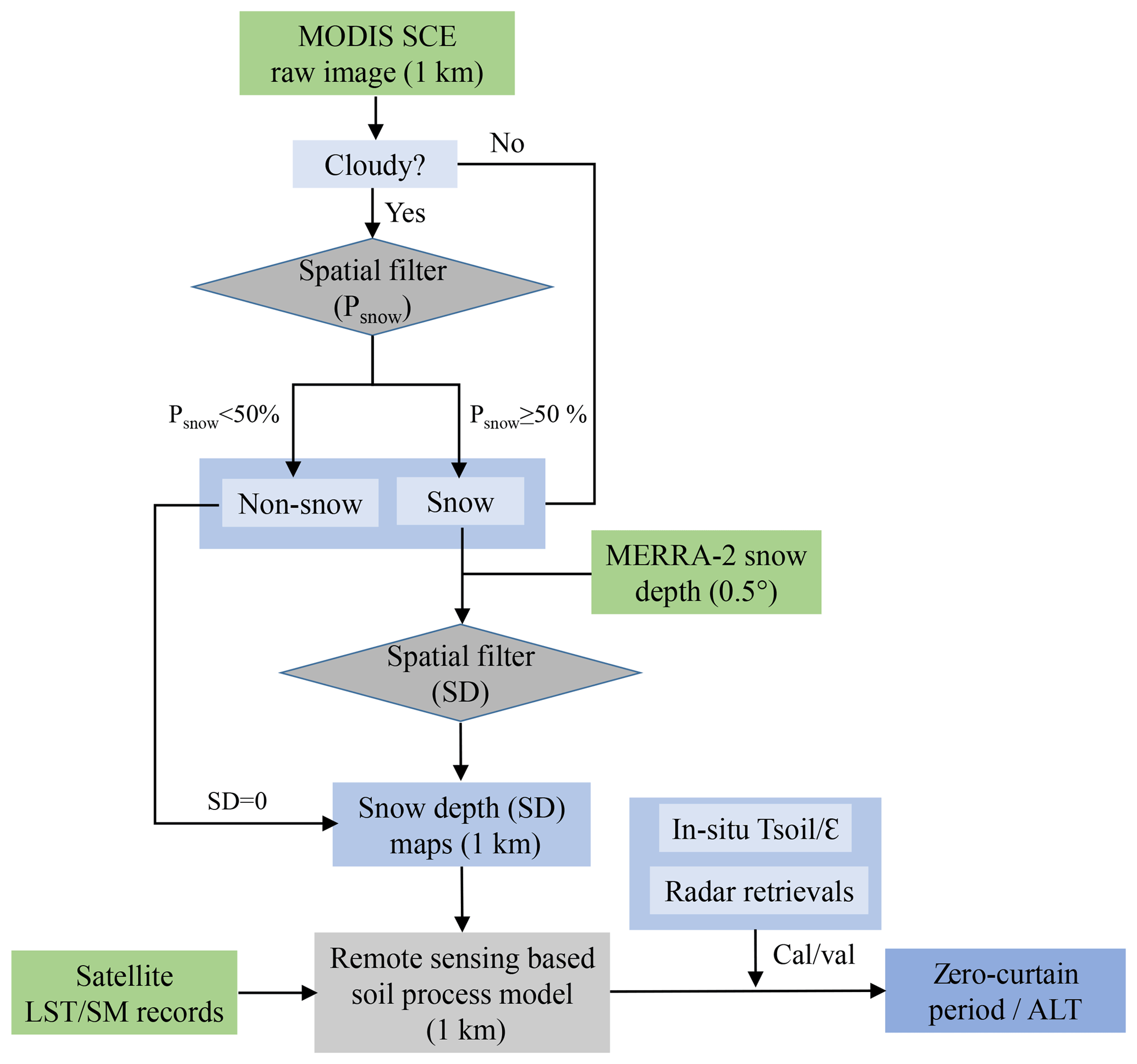
Figure 1Flow diagram describing the snow data processing and soil modeling procedure. A spatial filter was used to predict the snow occurrence probability for MODIS cloud-contaminated pixels. Based on the cloud-free MODIS SCE imagery, the snow depth of each snow-covered 1 km pixel was estimated from the snow depth of the neighboring MERRA-2 grid cells with weights predicted using another spatial filter. The downscaled 1 km snow depth data were then used to drive a remote-sensing-based soil process model to simulate the zero-curtain period and ALT. Both the snow data processing and soil modeling were carried out at an 8-day time step.
Soil dielectric constant is directly associated with the amount of unfrozen water remaining during soil freeze-up and thus may better define the active-layer freezing process compared with soil temperature. In this study, we investigated the sensitivity of soil dielectric constant to active-layer freezing indicated from both in situ measurements and airborne radar retrievals during the fall transitional period. Longwave (P-band) polarimetric SAR (PolSAR) data with large penetration depths (∼50–60 cm depending on soil moisture content) were acquired from airborne radar acquisitions over northern Alaska in August and October 2014 and 2015 prior to the NASA Arctic Boreal Vulnerability Experiment (ABoVE) airborne campaign. The airborne radar data were used to characterize spatial variability and seasonal shifts in the near-surface ( cm depth) soil dielectric constant associated with the soil F–T transition. These data were used to augment more detailed but spatially limited in situ soil dielectric measurements used for model parameterization and to assess the value of longwave radar measurements in frozen soil studies. Resulting model simulations were then validated using ground-based zero-curtain measurements. We then conducted an integrated analysis of the sensitivity of active-layer freezing to variable snow conditions combining in situ observations, model simulations and airborne radar retrievals.
2.1 Constructing a fine-resolution regional snow data set
In a previous study (Yi et al., 2018) we used coarse-resolution (0.5∘) snow depth data from the MERRA-2 global reanalysis as input for the permafrost model over Alaska. In the prior study, we first interpolated the MERRA-2 data over a finer 1 km spatial grid using an inverse-distance weighting scheme and then used the MODIS 500 m SCE data to identify snow-free pixels within each coarser MERRA-2 grid and adjust the 1 km snow depth estimates accordingly. However, a more sophisticated downscaling scheme was needed to better account for the influence of local topography on the 1 km snow distribution pattern. This information can be derived from the MODIS SCE data; however, persistent cloud cover and patchy snow conditions constrain the ability of the MODIS SCE data to capture snow cover variability, especially during the transitional season. To overcome this constraint, in this study we developed an elevation-based spatial filtering algorithm to predict the snow occurrence for MODIS cloud-contaminated pixels; we then used the cloud-free MODIS SCE data to downscale the MERRA-2 snow depth data (Fig. 1). For each snow-covered 1 km pixel indicated by the MODIS data, we estimated the snow depth based on the snow depth of neighboring MERRA-2 0.5∘ grid cells, with weights predicted using a similar spatial filter.
2.1.1 Cloud filtering of MODIS SCE data
Most existing cloud-filter algorithms designed for the MODIS SCE products use empirical relationships between snow cover conditions and ancillary data to predict the snow cover occurrence for cloud-covered pixels (e.g., Parajka and Blöschl, 2008; Gafurov and Bárdossy, 2009; Parajka et al., 2010). The empirical relationships are generally appropriate for the limited areas or conditions in which they were developed and may not be suitable for other regions with different climates or topography. To develop a more general cloud-filter algorithm, we exploited spatial interpolation methods originally designed for generating grid-based surface meteorology from in situ weather station observations. We used a similar methodology that was used to generate Daymet surface precipitation, which uses a truncated Gaussian weighting filter and accounts for the dependence of precipitation on elevation (Thornton et al., 1997). This method was found to generate reliable precipitation estimates in complex topography in the western USA (Henn et al., 2018). For our application, we treated the pixels without cloud cover as “station observations” and then used the spatial filter to predict the occurrence of snow in cloud-contaminated pixels and generate continuous cloud-free snow cover images at 1 km spatial resolution and 8-day timescale.
The general form of the spatial filter, with respect to the cloud-contaminated or central pixel (i) to be filled, is defined as follows:
where W(d) is the filter weight associated with the radial distance d from the central pixel, and α is a unitless shape parameter with a prescribed value of 6.0 following Thornton et al. (1997). R is the truncation distance, varying with the local density of observations (i.e., cloud-free pixels) in the adjacent areas of the central pixel; at least 50 observations should be included for interpolation to the central pixel, within a maximum search radius of 50 km. Snow distribution is closely associated with local topography; therefore, we divided the observations falling within the range of the search radius into two groups representing elevations above and below the elevation of the central pixel. We then estimated the snow occurrence probability (Psnow) and weighted elevation (Z) for each group:
The snow occurrence probability at the central pixel (Psnow,i) was then estimated as a weighted function of the snow occurrence probability of the two groups (Zabove and Zbelow):
The snow cover condition (SC) of the central pixel is determined based on the comparison of Psnow,i with a specific cutoff value, Pcutoff:
Temporal filtering of the MODIS SCE data was conducted prior to the application of the spatial filter. Pixels with cloud cover were reclassified as either snow or nonsnow conditions if the two temporally adjacent 8-day periods were both identified as cloud-free and indicated consistent snow or nonsnow-covered conditions. Missing SCE pixels occurring during polar night were assigned as “snow” when there were established snow cover conditions in the prior 8-day period or there was more than 0.2 m snow depth indicated by the co-located MERRA-2 grid cell. This procedure effectively reduced the number of cloud-contaminated pixels requiring gap filling.
2.1.2 Downscaling of MERRA-2 snow depth data
The resulting cloud-free 8-day MODIS SCE data was used with a 1 km digital elevation model (DEM) aggregated from the 2 arcsec (∼60 m) DEM for Alaska (U.S. Geological Survey, 2017) to downscale the MERRA-2 snow depth data to 1 km resolution. Here, a spatial filter similar to the above procedure was used for the downscaling process, except that the MERRA-2 gridded snow data were treated as station observations and the station elevations were defined as the mean elevation within the associated MERRA-2 grid cell. Previous studies have demonstrated a clear dependence of snow depth on elevation, generally with a snow depth increase with elevation up to a certain level followed by a decrease at the highest elevations (Grünewald et al., 2014; Kirchner et al., 2014). Therefore, we used the transformed snow depth variables instead of the original MERRA-2 snow depth as input to the spatial filter to account for the dependence of snow distribution on elevation. We used a least-squares regression to analyze the relationship between snow depth and elevation:
The snow depth (SD) and elevation (Z) data were normalized using their maximum (SDmax and Zmax) and minimum (SDmin and Zmin) values from the MERRA-2 grid cells within the spatial search radius to account for local variability in snow distribution (Grünewald et al., 2014). β0 and β1 are empirical fitting parameters from the regression model. Linear regression does not account for the snow depth decrease at the highest elevations; however, the coarse MERRA-2 data represent average conditions within each ∼0.5∘ grid cell and are unable to capture snow depth changes at these high-elevation extremes.
For each 1 km snow-covered pixel indicated by the MODIS SCE data, snow depth is estimated as follows:
where the interpolation only weights MERRA-2 grid cells with snow occurrence (indicated by SC). The MERRA-2 snow depth data were used directly for the spatial interpolation (i.e., β1≅0) where no significant relationship was indicated between elevation and snow depth changes within the search radius.
2.2 The remote-sensing-driven permafrost soil process model
The newly developed snow depth data were used with other satellite remote-sensing data sets as primary input to an established permafrost soil model (Yi et al., 2018) for simulating soil freeze onset and zero-curtain period across Arctic Alaska. The model was developed based on a detailed permafrost hydrology model (Rawlins et al., 2013; Yi et al., 2015) but has a flexible structure designed to exploit remote-sensing observations as key model drivers and for model parameterization. The remote-sensing-based permafrost model, as described in Yi et al. (2018), uses a numerical approach to simulate soil F–T processes and the temperature profile down to 60 m below the surface using 23 soil layers, with increasing layer thickness at depth (soil nodes from 0 to 1 m: 0.01, 0.03, 0.08, 0.13, 0.23 ,0.33, 0.45, 0.55, 0.70, 1.05 m). Up to five snow layers are used to account for the effects of seasonal snow cover evolution on snow density and thermal properties. Both snow heat capacity and thermal conductivity vary with snow density and are estimated using empirical methods (Calonne et al., 2011). The model also accounts for the effects of organic soils and soil-water phase change on the soil F–T process as described below.
The soil model simulates snow and ground thermal dynamics by solving a 1-D heat transfer equation with phase change (Nicolsky et al., 2007; Rawlins et al., 2013):
where T(zt) is the temperature (∘C) at a specific soil depth (z) and time step (t), L is the volumetric latent heat of fusion of water (J m−3), ζ is the volumetric water content (m3 m−3), and θ is the unfrozen liquid water fraction (range: 0–1). C and λ are the volumetric heat capacity () and thermal conductivity () of soil respectively, varying with soil moisture, F–T state and depth. The upper boundary condition is set as the surface temperature (i.e., LST) at the snow–ground surface (zs), while a heat flux characterizing the geothermal gradient is applied at the lower boundary (zb). The soil heat capacity is a function of heat capacities for soil solid and liquid water, and ice components (Farouki, 1981):
where Cm, Co, Cw and Ci are the heat capacity of mineral and organic soil solid, liquid water and ice respectively, weighted by their volumetric function. f is the soil organic fraction; θsat, θw and θi are the respective saturated water content, volumetric liquid water and ice content, where . The thermal conductivity λ () was estimated as a normalized thermal conductivity of the dry (λdry) and saturated (λsat) soil thermal conductivity weighted by soil saturation:
where the Kersten number (Ke) is a function of the soil saturation degree, generally using a logarithm form for unfrozen soils or linear form for frozen soils (Lawrence and Slater, 2008). λdry is estimated from the soil bulk density; λsat is estimated as a geometric mean of the thermal conductivity of different soil components (Farouki, 1981), which can vary several-fold from pure organic soil (∼0.5 ) to mineral soils (1.5–3 ):
where λm, λo, λw and λi are the thermal conductivity of mineral and organic soil solid, liquid water and ice, respectively; and θsat,w and θsat,i are the respective unfrozen liquid water and ice fractions under saturated conditions.
The unfrozen liquid water fraction (θ) is estimated empirically as follows:
Soil water usually freezes at sub-zero temperatures depending on solute concentration and other factors, and the constant T∗ is used to represent this freezing-point depression, with values generally above −1 ∘C (Banin and Anderson, 1974; Woo, 2012). b is a dimensionless parameter determined by fitting the unfrozen water curve (Romanovsky and Osterkamp, 2000; Schaefer and Jafarov, 2016). A significant amount of liquid water can exist even when the soil temperature is considerably lower than T∗, characterized by different values of b. Fine-grained soils that can have a larger amount of liquid water below freezing are generally associated with smaller b values (Woo, 2012).
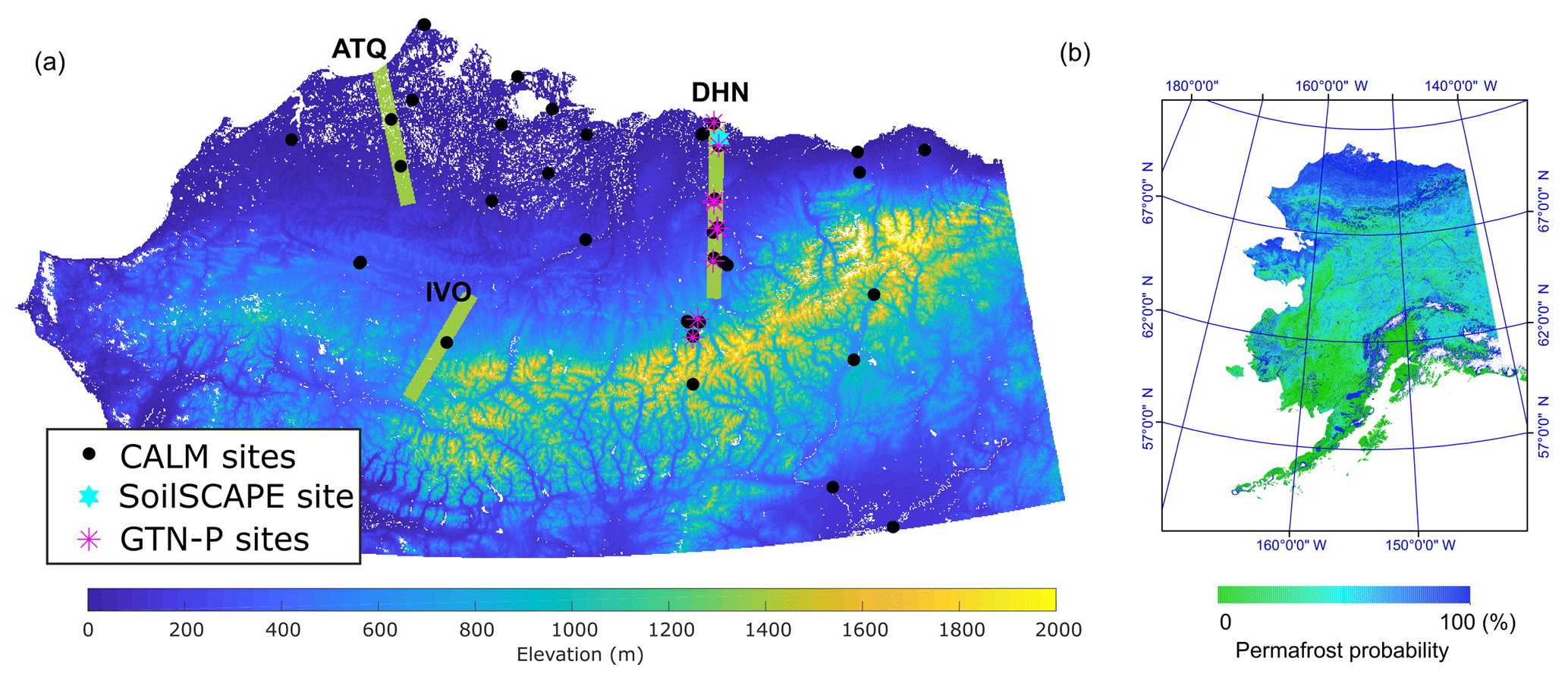
Figure 2(a) The study area (Arctic Alaska, >66.55∘ N) used for the soil model simulations and the locations of in situ sites used for model calibration and validation; (b) an Alaska permafrost probability map (Pastick et al., 2015) is also shown, indicating higher permafrost occurrence in Arctic Alaska. The in situ sites include the Prudhoe Meadow SoilSCAPE site, GTN-P soil temperature sites and CALM ALT sites. Airborne P-band radar data (denoted by green lines) were obtained in late August and early October in 2014 and 2015. Another radar flight line was collected over the Barrow area (not shown) but was not included in this analysis due to a large percent of surface water in this area.
2.3 Model driver data sets and in situ data
Model simulations were conducted in the Arctic Alaskan domain (>66.55∘ N, Fig. 2), encompassing an area of ∼ 400 000 km2 and spanning a 16-year period (2001–2016). Primary model drivers include MODIS 8-day composite 1 km LST (MOD11A2; Wan and Hulley, 2015) and 500 m SCE records (MOD10A2; Hall and Riggs, 2016), SMAP 9 km NatureRun (Version 4) and level 4 daily surface (≤5 cm depth) and root zone (0–1 m depth) soil moisture (L4SM, Reichle et al., 2017), and daily snow depth and snow density from MERRA-2 global reanalysis data (Gelaro et al., 2017). The MODIS LST and SMAP L4SM products were used to define model boundary conditions and soil thermal properties. The soil process model was run at 1 km resolution and 8-day time step consistent with the MODIS LST and SCE inputs. All model input data sets were reprojected to a consistent 1 km Albers projection. The model snow depth inputs were derived by combining the MODIS SCE and MERRA-2 snow depth records as discussed in Sect. 2.1. Compared with snow depth, snow density shows much smaller spatial and temporal variability (Sturm et al., 2010); therefore, we used the 1 km snow density data generated using a simple spatial interpolation scheme as described in Yi et al. (2018). Other ancillary inputs to the soil model included the 30 m National Land Cover Database (NCLD) 2011 (Jin et al., 2013), 2 arcsec (∼60 m) DEM for Alaska (U.S. Geological Survey, 2017), 50 m SOC estimates for Alaska (to 1 m depth; Mishra et al., 2016), and the global 9 km mineral soil texture data developed for the SMAP L4SM algorithm (De Lannoy et al., 2014). The dominant NLCD land cover type within each 1 km pixel was used to define the modeling domain, with open water and perennial ice and snow areas excluded from the model simulations. The soil texture and SOC data were used to define model soil properties including thermal conductivities and heat capacities. The SOC inventory data was distributed through the top 10 model soil layers (≤1.05 m depth) following an exponentially decreasing curve (Hossain et al., 2015) to calculate the SOC fraction and adjust the soil physical properties of each soil layer based on the weighted mineral and organic soil components. More details on the data processing can be found in Yi et al. (2018).
Three in situ data sets were used for model calibration and validation (Fig. 2), including half-hourly soil dielectric constant (ε) and temperature profile measurements from a Soil moisture Sensing Controller and oPtimal Estimator (SoilSCAPE) site (Moghaddam et al., 2010); daily soil temperature profile measurements from Global Terrestrial Network for Permafrost (GTN-P) sites (Biskaborn et al., 2015), and ALT measurements from regional Circumpolar Active Layer Monitoring (CALM) network sites (Brown et al., 2000). The SoilSCAPE soil temperature and ε measurements were obtained from four different depths (0.05, 0.15, 0.35, 0.56 m) and four different nodes of a wireless sensor network deployed near Prudhoe Bay, Alaska (70∘13′47 N, 148∘25′19 W) in the summer of 2016. ε was measured using a METER TEROS 12 soil moisture sensor operating at 70 MHz. For the GTN-P in situ measurements, we only selected the sites where shallow ground-temperature measurements (generally down to 1 m depth) were available for at least 2 consecutive years. Most GTN-P sites meeting these criteria in Arctic Alaska are located along the Dalton Highway (Table S1 in the Supplement). In addition, daily snow depth measurements using an ultrasonic sensor were available at SNOTEL (SNOwpack TELemetry) sites across Alaska (Schaefer and Paetzold, 2000; http://www.wcc.nrcs.usda.gov, last access: 1 September 2018, Fig. S1 in the Supplement) and used to validate the 1 km snow depth product (Sect. 2.1).
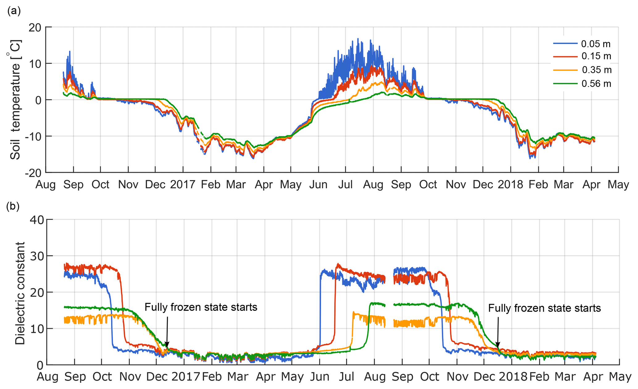
Figure 3In situ measurements of soil temperature (a) and dielectric constant (b) for a single SoilSCAPE sensor node (S6) at the Prudhoe Meadow site in northern Alaska (http://soilscape.usc.edu, last access: 1 May 2018).
2.4 Model parameterization
Soil dielectric properties are strongly correlated with soil moisture, texture and F–T state (Mironov et al., 2010); ε can capture the soil-freezing process well due to large ε differences between liquid water and ice (Dobson et al., 1985), especially during the zero-curtain period, when soil temperatures hover around 0 ∘C and are a relatively poor indicator of F–T conditions (Fig. 3). The SoilSCAPE measurements were used to calibrate the model unfrozen water content curve (Eq. 11) assuming a linear relationship between ε and liquid water content (Mironov et al., 2010; Park et al., 2017). However, the slope of this linear relationship may change during the freezing period due to different dielectric properties of free and bound water, and ice (Mironov et al., 2010). The ε measurements were also used to determine the timing of complete soil freeze-up at each soil depth. The timing of soil freeze-up was defined when the observed ε drops below a critical level:
where εmax and εmin are the maximum and minimum dielectric constants for each soil layer, and the threshold δ is an empirical parameter. The zero-curtain period at different depths was then calculated as the difference between soil freeze-up and land-surface freeze onset. The land-surface freeze onset was determined from MODIS 1 km LST records extracted at the SoilSCAPE site and defined as the date at which the mean LST during three consecutive 8-day periods dropped below 0 ∘C.
The model-simulated soil temperature profile is very sensitive to the soil thermal conductivity, largely determined by soil texture (organic or mineral soils) and soil saturation (Eqs. 9–10), which are also two major factors affecting ε. Therefore, we used the in situ ε data at the SoilSCAPE site to guide the parameterization of model soil thermal properties. Since the soil is mostly saturated at this site, much larger ε values in the top two layers during the thaw season (Fig. 3) should be related to organic-rich soils with large soil porosity (thus high volumetric soil moisture). We defined the top five model soil layers (0–0.23 m) as organic soils and adjusted the model soil thermal properties accordingly. The unfrozen soil thermal conductivity within the organic layer was assumed to gradually increase with depth from ∼0.5 in the surface organic soil layer to ∼1.2 at 0.33 m depth for mineral soils, accounting for increases in the soil bulk density (Letts et al., 2000). Similarly, soil porosity was assumed to gradually decease from 0.8 at the surface to ∼0.4 in the deeper mineral soil layers. The soil thermal conductivity for frozen conditions can then be determined from Eq. (10). Using this soil thermal conductivity profile, the model-simulated temperatures agree well with the in situ observations (R>0.97, RMSE<2.24 ∘C for all measured soil depths). We then tested different soil dielectric thresholds (δ) ranging from 0 % to 50 % and selected the threshold that produced minimum bias and RMSE between the zero-curtain period determined using in situ ε measurements and model-simulated unfrozen water content. Using this trial and error method, an optimal threshold of 15 % was selected, which produced a mean RMSE of 10.3 days in the simulated zero curtain from 0.15–0.56 m soil depth in 2016 and 2017 (Fig. 4a).
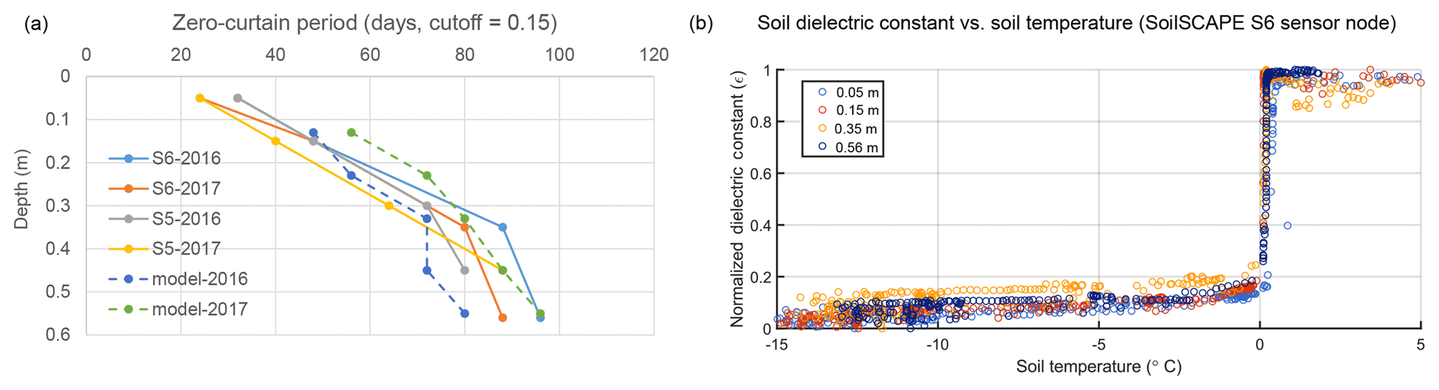
Figure 4Soil-freezing characteristics at the Prudhoe Meadow SoilSCAPE site: (a) comparisons of modeled and observed zero-curtain period at two sensor nodes (S5 and S6) using a cutoff threshold of 0.15 (Eq. 12) for both in situ soil dielectric constant and model-simulated unfrozen water content to determine soil freeze onset; (b) changes in in situ soil dielectric constant during soil freezing at the S6 node. The soil dielectric constant was normalized using the maximum and minimum values of soil dielectric constant during the observation period.
The resulting threshold δ was then used to determine the critical threshold of soil temperature at soil freeze-up using both the GTN-P measurements and soil model simulations. The observed changes in the normalized ε with soil freezing is presented for a selected SoilSCAPE sensor node (S6) in Fig. 4b. ε below the freezing point and above −10 ∘C ranges from ∼5 % to 20 % of the ε value for unfrozen soils. Assuming a linear relationship between ε and liquid water content (Mironov et al., 2010), Fig. 4b can approximate changes in unfrozen water content during soil freezing. Assuming soil freeze-up starts when ε drops below 15 %–20 % of the annual amplitude, the corresponding soil temperatures range from −0.01 to −1 ∘C at depths between 0.05 and 0.56 m. We selected a temperature threshold of −0.35 ∘C for soil freeze-up, which is at the higher end of the range indicated from the S6 node, but closer to the other SoilSCAPE nodes showing more rapid ε changes below 0 ∘C. This temperature threshold is also consistent with our model simulations, which show a −0.3 to −0.5 ∘C temperature range and 15 %–20 % liquid water content during freeze-up. This temperature threshold was used to determine the soil freeze onset and zero-curtain period at the GTN-P sites with only soil temperature measurements available. However, there is large variability in the relationship between ε and liquid water content at freezing temperatures due to changes in free and bound water and ice components (Mironov et al., 2010; Naeimi et al., 2012), which can result in large uncertainties in the above estimated thresholds.
2.5 Soil dielectric constant retrievals from airborne P-band radar
The soil model unfrozen water content curve used to define the soil freeze-up and zero curtain was only calibrated using limited SoilSCAPE soil dielectric measurements. We therefore evaluated the sensitivity of surface soil dielectric properties derived from local-scale (∼50 m) airborne low-frequency (P-band) radar acquisitions along regional transects in northern Alaska and associated F–T patterns to snow cover variations. Multiple flight lines were acquired in late August (fully thawed) and early October (partially frozen) of 2014 and 2015 in northern Alaska, including a regional transect along the Dalton Highway (DHN, 148.39–149.05∘ W, 68.78–70.40∘ N). Multiple soil parameters, including active-layer thickness (ALT) and soil moisture (converted from soil dielectric constant), were derived from NASA Airborne P-band (430 MHz) PolSAR radar backscatter measurements in August and October (Chen et al., 2019). The radar soil retrievals examined in this study differ from Yi et al. (2018), which used active-layer retrievals derived from multi-frequency (L + P-band) radar backscatter acquired in October 2015. The alternative single-channel (P-band) time series algorithm used in the current study avoids potential artifacts introduced from variable P and L-band radar acquisition times. The soil parameters were derived from the radar backscatter using a three-layer soil dielectric model. In August, the three layers represent the surface thawed layer, middle and bottom active layer, and the top of the upper permafrost layer. In October, the two surface layers represent a partially frozen active layer with a frozen surface layer overlying a deeper unfrozen active layer. An iterative optimization scheme was used to estimate the soil parameters by minimizing differences between the observed radar backscatter and radar scattering model simulations using the above three-layer soil dielectric model. The retrieved parameters include the thickness and soil dielectric constant of the surface layer in August and October, the depth and dielectric constant of deeper active layer. Initial validation indicated favorable radar ALT retrieval accuracy in relation to in situ CALM measurements along the DHN transect (Chen et al., 2018, 2019). The differences in surface soil dielectric constant between August and early October represent the changes in soil liquid water content that occur during F–T conditions. Therefore, we examined differences in soil dielectric constant under variable MODIS snow cover fraction to clarify the influence of snow cover on active-layer freezing.
2.6 Regional soil model simulation and analysis
We conducted an integrated analysis of in situ ground observations, soil model simulations and airborne radar retrievals to investigate the sensitivity of soil freezing to variable snow cover conditions across Arctic Alaska. For the regional simulation, the soil process model was spun up for 50 years to bring the top 10 m soil temperature profile into dynamic equilibrium using model inputs in the year 2000 (Yi et al., 2018), followed by a model transit run from 2001 to 2017. Unfrozen conditions in the deeper active layer may persist well into the winter season and into the subsequent calendar year. In order to accurately estimate the active-layer freeze onset and zero-curtain period for the current year, model simulations of the next calendar year were also needed. Therefore, the soil freeze onset and zero-curtain period in year 2017 were not calculated. The soil freeze onset for each soil layer was determined when model-simulated soil temperature dropped below −0.35 ∘C as discussed in Sect. 2.4. The zero-curtain period at each soil depth was defined as the duration between land-surface freeze onset and freeze onset of the given soil layer. The regional correlation between snow onset calculated from the MODIS SCE data and the zero-curtain period for each soil layer was used to examine relations between the timing of early snow accumulation and soil freeze-up. Snow onset was determined as the center of the 8-day period with more than three adjacent snow-covered periods within a 40-day moving window; the relatively long temporal window was used to account for more variable snow cover conditions during fall.
We selected the DHN flight transect as the focus area for the integrated analysis due to the relatively dense network of GTN-P soil temperature and CALM ALT sites in this area relative to other transects (i.e., ATQ and IVO, Fig. 2). Because the MODIS 8-day SCE product (i.e., MOD10A2) only provides binary snow data (i.e., snow vs. nonsnow), the data set was binned for each 0.1∘ latitudinal region along the radar flight transect to calculate the snow-covered area fraction (SCF). We also averaged the airborne radar-retrieved surface soil dielectric constant for each 0.1∘ latitudinal bin and analyzed the correlations between SCF and selected variables representing the soil-freezing process, including the radar-retrieved surface dielectric constant changes between October and August, and the zero-curtain period derived from both the soil model simulations and in situ data. For the site analysis, the SCF from the 0.1∘ latitudinal bin including the site was used. Arctic Alaska is generally fully snow covered by the end of October or early November. Therefore, we used the SCF averaged from September to October for the zero-curtain analysis, while only the September SCF was used for the airborne radar data analysis, since the radar data were obtained in early October.
3.1 Model validation
Accurate simulation of early cold-season soil freezing requires accurate characterization of landscape-scale snow cover conditions, which was addressed in this study by gap filling the MODIS SCE record to mitigate data loss from pervasive cloud cover and other factors. The gap-filled MODIS SCE products were then combined with other ancillary data to downscale the MERRA-2 reanalysis snow depth data, as one of the main driver data sets for the permafrost soil model. The accuracy of the gap-filled MODIS SCE product was cross-checked using the two MODIS sensors (Terra and Aqua); the downscaled snow depth data were evaluated using in situ SNOTEL observations across Alaska. The model-simulated soil-freezing process and ALT dynamics were conducted over a smaller Arctic Alaska domain and evaluated using a diverse set of regional observations.
3.1.1 Regional 1 km snow cover product
The cloud-free Aqua MODIS SCE data were used to evaluate the accuracy of filled pixels identified as cloud covered in the Terra MODIS SCE data and vice versa, assuming relatively consistent snow conditions between morning (Terra) and afternoon (Aqua) SCE acquisitions during the 8-day composite period. Our results indicate an accuracy of more than 80 % in the cloud-filtering algorithm with no obvious differences observed between the two sensor SCE records (Table 2 and Fig. S2). The cloud cover fraction for the 8-day temporal composite Terra MODIS SCE data represents 0.5 % to 10.1 % of the entire state throughout the year, and the percentage of cloud-free Aqua MODIS pixels that overlapped with cloud-covered Terra MODIS pixels ranges from 0.4 % to 4.6 % (Fig. S2). There are significantly more cloud-covered pixels in the Aqua MODIS record (1.1 %–15.2 %) and thus more cloud-free Terra MODIS pixels (0.9 %–9.8 %) overlapping with cloud-covered Aqua MODIS pixels. Cloud cover mostly occurs in the spring and fall shoulder seasons, resulting in larger SCE uncertainties during those periods. There is no obvious bias in the misclassification of cloud-contaminated pixels (Table 2), which indicates that using a cut-off threshold of 50 % for the snow occurrence probability (Pcutoff, Eq. 4 and Table 1) to classify snow or nonsnow conditions works well. Using a higher threshold (e.g., 60 %) generally results in more snow pixels misclassified as land pixels and vice versa.
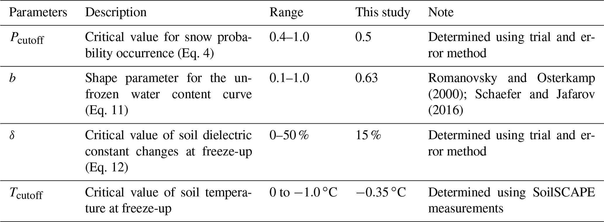
Table 2The accuracy of the spatial filter algorithm applied to the Aqua MODIS SCE data during spring (April to June) and fall (September to November) transitions averaged over Alaska from 2003 to 2015. Pixels that identified cloud contamination in the Aqua MODIS record but indicated clear conditions in the Terra MODIS were used for evaluation. The percentage of cloud-contaminated and evaluated pixels were calculated for the entire Alaska domain, while the accuracy and misclassification were calculated as the percentage of the evaluated pixels. Both Terra and Aqua MODIS SCE data show similar accuracy, while only the Aqua MODIS results are shown here due to a higher percentage of cloud-contaminated pixels (available for evaluation) in the Aqua imagery.
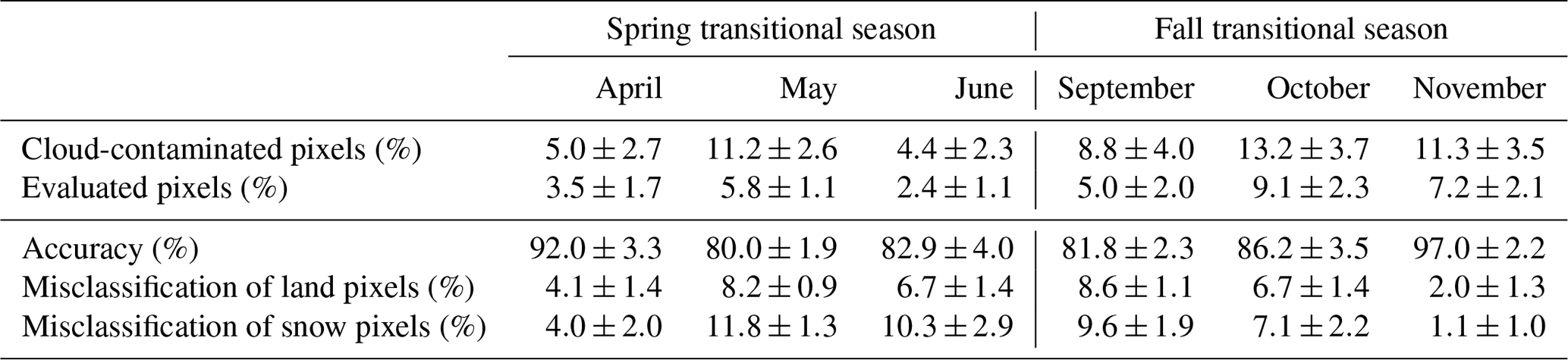
Table 3Statistics of 1 km MERRA-2 snow depth data generated using different spatial interpolation schemes compared with in situ snow depth measurements at the Alaskan SNOTEL sites.
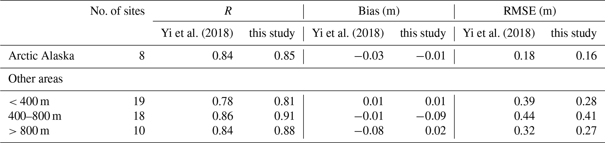
Compared with in situ snow depth measurements from the Alaskan SNOTEL sites, the 1 km MERRA-2 snow depth data generated using the new downscaling algorithm showed an overall improvement compared to the original spatial interpolation scheme used in Yi et al. (2018) (Table 3). The new 1 km snow depth data showed overall reduced RMSE and lower bias except in Interior Alaska at elevations between 400 and 800 m. At these elevations the USGS DEM used for spatial downscaling at the 1 km grid shows large deviations from the reported SNOTEL site elevations (Fig. S3), which may account for the relatively poorer performance of the new snow depth data set in this elevation band. In Arctic Alaska, the new snow depth product has a modest improvement over the Yi et al. (2018) product, with an RMSE of 0.16 m and bias of −0.01 m versus an RMSE of 0.18 m and bias of −0.03 m for the original data set. However, there are only eight SNOTEL sites in this region and only two sites at the Alaska North Slope. Compared with the Yi et al. (2018) product, the new MERRA-2 downscaled snow product captured more fine-scale details of spring snow melting and topographically varying snow distribution, especially in mountain areas (Figs. 5 and S4).
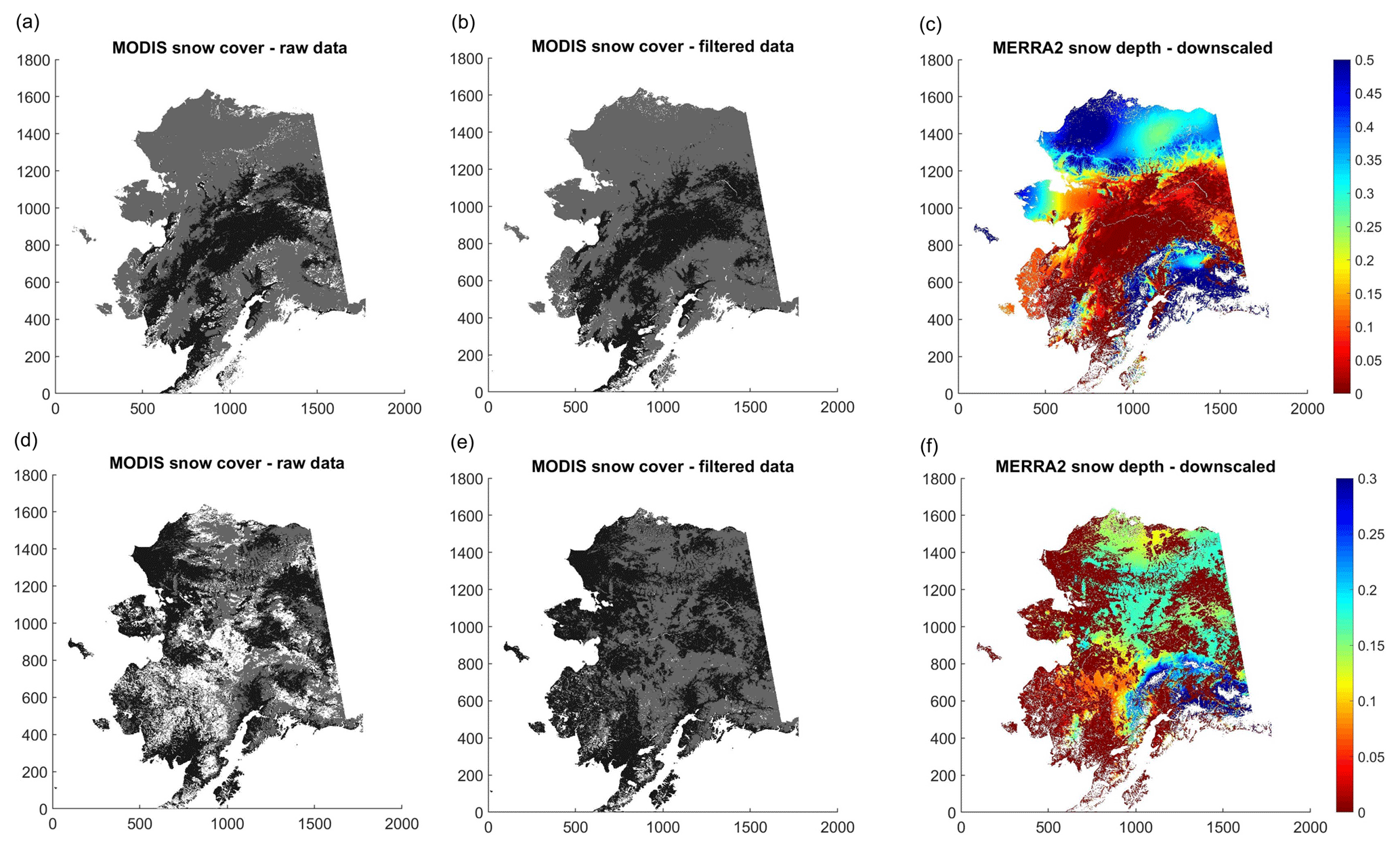
Figure 5Illustration of the snow data processing: the raw (a, d) and cloud-filtered (b, e) MODIS SCE images using an elevation-based spatial filter and downscaled MERRA-2 snow depth (in meters) data (c, f) using the filtered MODIS SCE and DEM data during spring snow melt (a–c: 23–30 April) and early snow accumulation (d–f: 30 September–7 October) period in 2007. In the MODIS images, snow-covered areas are shown in gray, while land and cloud-covered areas are shown in black and white, respectively.
The snow offset and onset derived from the MODIS SCE and downscaled MERRA-2 snow depth records show very similar spatial patterns and trends over the 2001 to 2016 study period (Figs. S5 and S6). These results indicate that the downscaled MERRA-2 snow depth data generally capture the regional variability in snow cover conditions during the transitional season indicated from the MODIS observations. During the study period, the data sets show similar spring snow offset dates over Alaska (e.g., DOY 138±7 for MODIS versus DOY 140±7 for downscaled MERRA-2 snow depth), while there is an approximate 10-day difference in fall snow onset dates between the two data sets (MODIS: DOY 284±5; MERRA-2: DOY 273±5). The difference in mean snow onset is likely due to different methods used to determine snow onset for the two data sets. For the MODIS SCE record, snow onset was chosen as the composite period with more than three adjacent 8-day snow-covered periods within a 40-day moving window, while snow onset was defined from the downscaled snow depth record as the composite period with a mean snow depth above a 0.05 m threshold within a 24-day moving window. A higher snow depth threshold results in a later snow onset date in the MERRA-2 data set. However, the two records show similar snow onset patterns (Fig. S5) and interannual variability during the study period (R=0.79, p<0.01). Both data sets show a generally earlier snow onset trend in Arctic Alaska over the study period, which is discussed in Sect. 3.2.
Table 4Comparisons of model-simulated and in situ observed zero-curtain period at 0.35 m soil depth for sites along the DHN transect. The model-simulated mean zero-curtain period was calculated from 2001 to 2016. The zero-curtain period calculated using in situ soil temperatures at closely adjacent sites (e.g., the three Franklin Bluff sites, Table S1) were combined for a longer observational record.
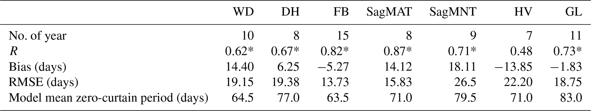
Note that the asterisk denotes p<0.1, WD is West Dock, DH is Deadhorse, FB is Franklin Bluffs, SagMAT is Sagwon MAT, SagMNT is Sagwon MNT, HV is Happy Valley and GL is Galbraith Lake. Imnaviat 1 and GL were closely adjacent sites and were combined to form a longer time series.
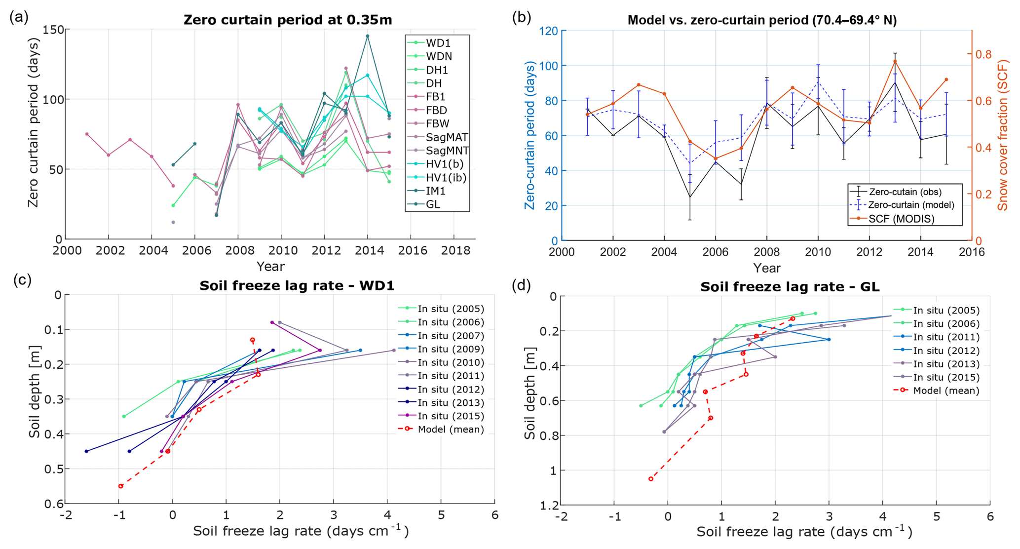
Figure 6Comparisons of soil-freezing characteristics derived from GTN-P soil temperature measurements and model simulations along the DHN transect in northern Alaska: (a) interannual variations in zero-curtain period derived from in situ measurements, (b) variations of model versus in situ zero-curtain period at 0.35 m soil depth relative to MODIS SCF averaged for the northern part of the DHN transect, (c, d) changes in the soil freeze lag rate with depth at two DHN sites. Both sites have lower ALT in the earlier years shown here, ranging from 0.37 m in the earlier period to 0.43 m during later period of record for the WD1 site and from 0.47 to 0.57 m for the GL site.
3.1.2 Soil model simulations
Across the DHN transect, the soil model-simulated zero-curtain period was significantly (p<0.1) correlated with the in situ observations, with a mean bias of 6.6 days and RMSE of 19.0 days at 0.35 m soil depth (Table 4). However, lower correspondence was found between the model simulations and in situ observations at the DHN Happy Valley site (R=0.48, p>0.1). Relatively large RMSE differences in the estimated zero curtain period were mainly due to large interannual variability in the soil freeze onset and zero-curtain period during the study period (Fig. 6a). Both model-simulated and in situ observed zero-curtain periods were strongly correlated at different soil depths (e.g., R>0.92 at 0.25 and 0.35 m), except for the SagMAT site (R=0.87). Larger differences were observed in the model-simulated and in situ observed zero-curtain period at the surface (≤0.15 m) and for deeper soil layers (≥0.45 m) due to model limitations in capturing a shorter zero-curtain period in surface soils on an 8-day temporal scale, and larger uncertainties in both the in situ observations and model-simulated zero-curtain period in deeper soils. Across the DHN transect, both the model-simulated and in situ observed soil freeze onset were strongly correlated (R>0.9) with the zero-curtain period at soil depths below 0.15 m (Figs. 6a, S7–S8); therefore, the modeled soil freeze onset was not discussed separately. The in situ observations also showed consistent interannual variability in the soil freeze onset and zero-curtain period across the GTN-P sites within the DHN transect, which spans an approximate 2∘ latitudinal gradient (Table S1); the correspondence was particularly strong for sites located north of the Sagwon site (>69.43∘ N), which is discussed further in the next section (Sect. 3.2.1).
Across Arctic Alaska, model simulations slightly overestimate ALT compared with the available in situ ALT measurements from 32 CALM sites, with a mean bias of 10.0±13.2 cm (∼20 % of mean ALT), and an RMSE of 15.6±7.7 cm. For the 23 CALM sites with at least 9 years of ALT measurements, the correlations between model-simulated ALT and the in situ measurements range from 0.20 to 0.69, with 17 (73.9 %) of the sites showing significant correspondence (p<0.1).
3.2 Sensitivity of active-layer freezing to snow cover
We first analyzed the sensitivity of active-layer freezing to seasonal snow cover using in situ observations, local-scale airborne P-band radar retrievals, MODIS snow cover observations and model simulations, focusing on the DHN transect in the Alaska North Slope. We then evaluated the regional sensitivity of model-simulated soil freeze onset and zero-curtain period within the active-layer to early snow accumulation indicated by the MODIS SCE record across Arctic Alaska.
3.2.1 Integrated analysis along the DHN airborne flight transect
For all sites along the DHN transect, both the model-simulated and in situ observed zero-curtain periods at 0.25 and 0.35 m soil depths showed significant positive correlations (, p<0.1) with MODIS SCF. The zero-curtain period and SCF record showed similar interannual variability across the DHN transect, particularly north of Sagwon sites (>69.4∘ N). Thus years with greater (less) snow cover are associated with a generally longer (shorter) zero-curtain period at these depths. The average zero-curtain period at 0.35 m soil depth for the DHN transect sites located from 70.4 to 69.4∘ N is shown along with the corresponding MODIS SCF observations in Fig. 6b. These observations show large interannual variability in early season snow accumulation in this area, with the fall (September–October) SCF varying from 0.35 to 0.77 from 2001 to 2015. Correspondingly, both the in situ and model-simulated zero curtain show large variability throughout the study period; here, the in situ observations varied from 23.5 to 79.2 days at 0.25 m and from 24.7 to 90.3 days at 0.35 m, while the model simulations ranged from 29.3 to 76.0 and 44.0 to 90.7 days for the same soil depths.
The timing of early snow accumulation was the primary factor affecting the freezing process of the top soils, while ALT is more closely related to the length of zero-curtain period in deeper soils, particularly in areas with a shallower thaw depth. This can be seen from the delayed soil freezing below 0.30 m soil depth at two monitoring sites (West dock and Galbraith Lake) in years with larger ALT (Fig. 6c–d). Both monitoring sites show deeper ALT conditions during the later years of the study period, which are also associated with larger soil-freezing lag rates. Here, the soil-freezing lag rate is defined as the ratio of the soil freeze onset difference between two adjacent soil layers and the respective depth difference between the two layers. However, soil-freezing lag rates derived from both the in situ measurements and model simulations show large variability and are likely associated with large uncertainty, especially for deeper soil layers. The temporal coverage of the in situ observations used for estimating the soil parameter conditions is also less extensive than the model simulations, which may contribute additional uncertainty.
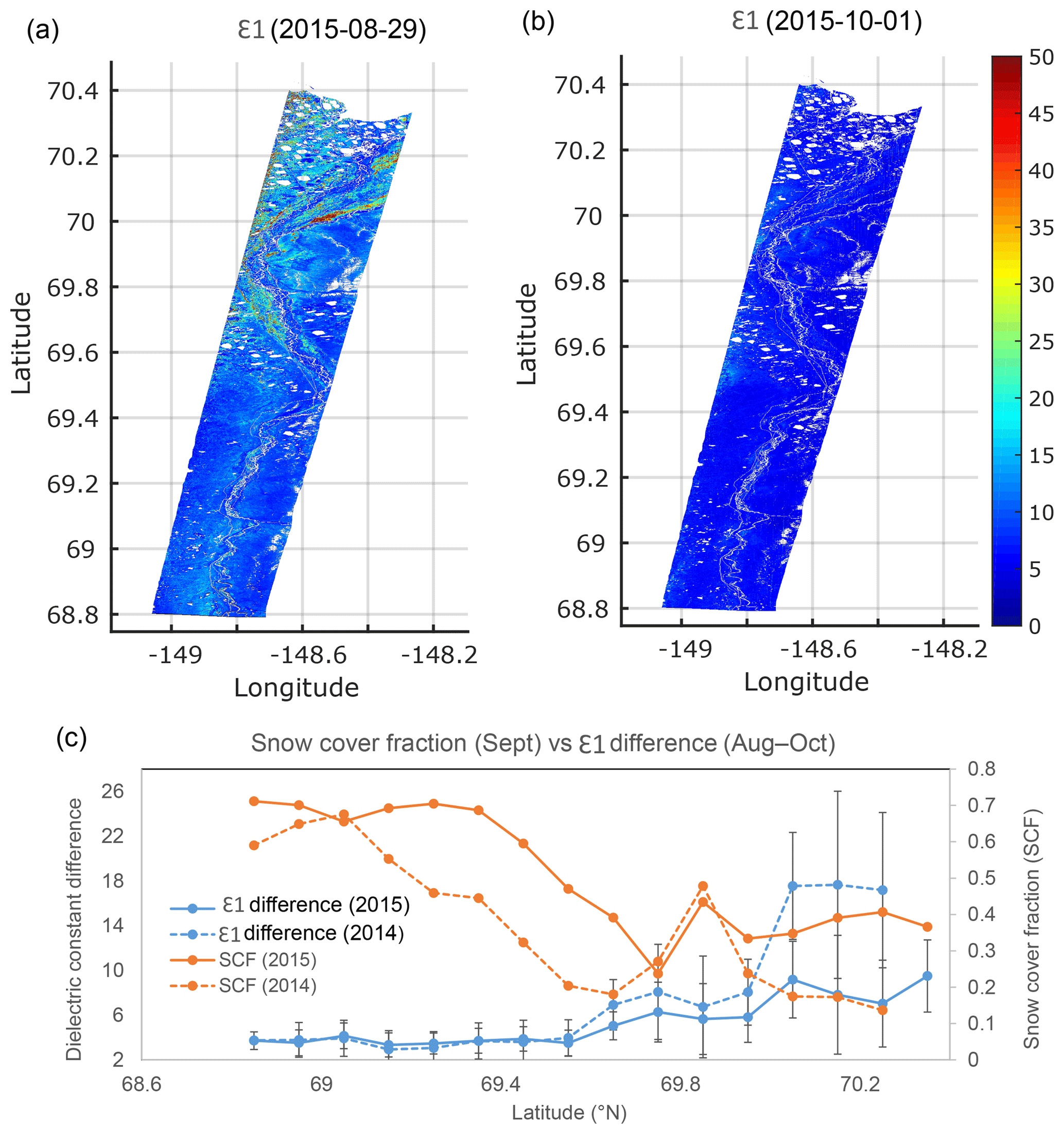
Figure 7Soil-freezing process indicated by the radar-retrieved (Chen et al., 2019) soil dielectric constant (ε1) of surface soils ( m) at the DHN transect in August (a) and October (b), and changes in ε1 in relation to MODIS SCF (c). The ε1 differences between August and October were binned to 0.1∘ latitudinal bins, while SCF was calculated as the percentage of snow-covered pixels indicated by MODIS SCE data for each 0.1∘ bin. The standard deviations of ε1 differences for each 0.1∘ bin were shown as error bars.
The airborne P-band radar retrievals over the DHN flight transect in early October (9 October in 2014, 1 October in 2015) showed a larger reduction in the surface soil dielectric constant (ε1) in areas with shallower snow cover during September than areas with deeper snow conditions (Fig. 7). In both years, the ε1 differences were negatively correlated with MODIS SCF across the DHN latitudinal gradient (2014: , 2015: , p<0.01, n=17). The reduction in ε1 retrievals in early October was more obvious in the northern part (>69.5∘ N) of the transect (2014: , 2015: ), which had a shallower seasonal snow cover (mean SCF of 0.22 in 2014 and 0.38 in 2015) and relatively early onset of frozen conditions than the southern part of the transect. Variation in vegetation cover may also contribute to the large contrast in the ε1 retrievals between the northern and southern portions of the transect, though the large apparent changes in ε1 between 2014 and 2015 in the northern portion of the transect provide a relatively robust indicator of frozen soil conditions. A similar relationship between radar-retrieved dielectric constant changes and MODIS SCF was observed over the Atqasuk (ATQ) flight transect. However, the opposite pattern was observed over the Ivotuk (IVO) transect, where ε1 changes increased with increasing seasonal snow cover at higher elevations (Fig. S9). The IVO transect differs from the other Alaska tundra transects by encompassing more variable topography (Fig. 2) and higher elevations (614±75 m) than both DHN (208±36 m) and ATQ (34±7 m).
Figure 8Model-simulated zero-curtain period at 0.35 m in relation to snow accumulation during the early snow season indicated by filtered MODIS SCE images for 2 selected years with later (2007: a–c) and earlier (2015: d–f) snowfall. In the MODIS images, snow was shown in dark gray, while land was shown in black and the areas masked out were shown in white.
3.2.2 Model sensitivity analysis in Arctic Alaska
We first compared the model-simulated zero-curtain period over Arctic Alaska for 2 selected years with relatively late (2007) and early (2015) snowfall. These results indicate that snow accumulation during the early cold season is a primary control on the zero-curtain period within the upper (<0.4 m) soil layers (Fig. 8). The regional mean surface freeze onset and snow onset based on the MODIS LST and SCE observations was DOY 269±5 (surface freeze onset) and 281±9 (snow onset) in 2007, and DOY 259±8 (surface freeze onset) and 262±12 (snow onset) in 2015. The later snow cover establishment in 2007 resulted in an overall shorter zero-curtain period over most of the Arctic Alaska region, with a model-simulated mean zero-curtain period of 49.3±25.1 days at 0.25 m depth and 64.3±26.3 days at 0.35 m depth. In contrast, earlier snow accumulation in 2015 resulted in a longer zero-curtain period, ranging from 69.4±22.1 days at 0.25 m depth to 84.7±25.2 days at 0.35 m depth. The spatial pattern of the model-simulated zero-curtain period also corresponded well with the snow accumulation pattern indicated from the MODIS SCE observations, leading up to full snow cover conditions.
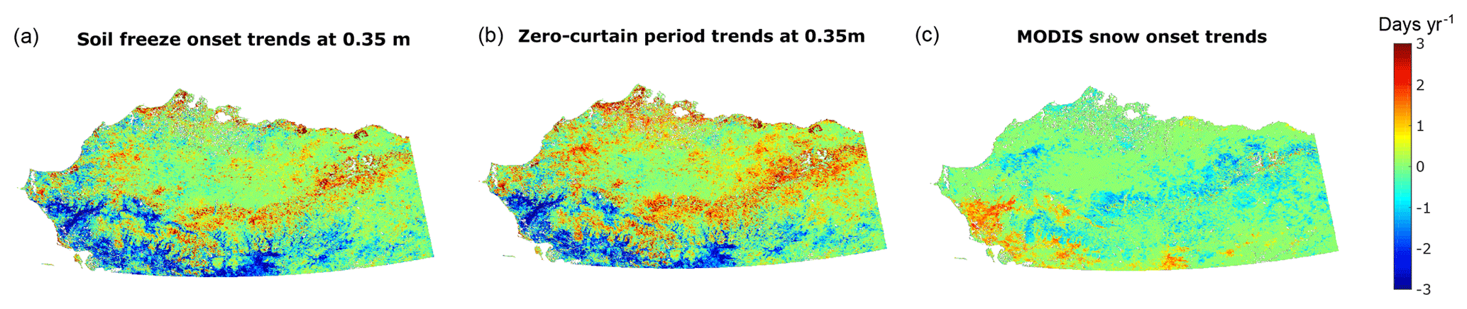
Figure 9Trends in model-simulated soil freeze onset (a) and zero-curtain period (b) at 0.35 m depth from 2001 to 2016. The fall snow onset trend for the same period derived from the MODIS SCE data is shown in (c).
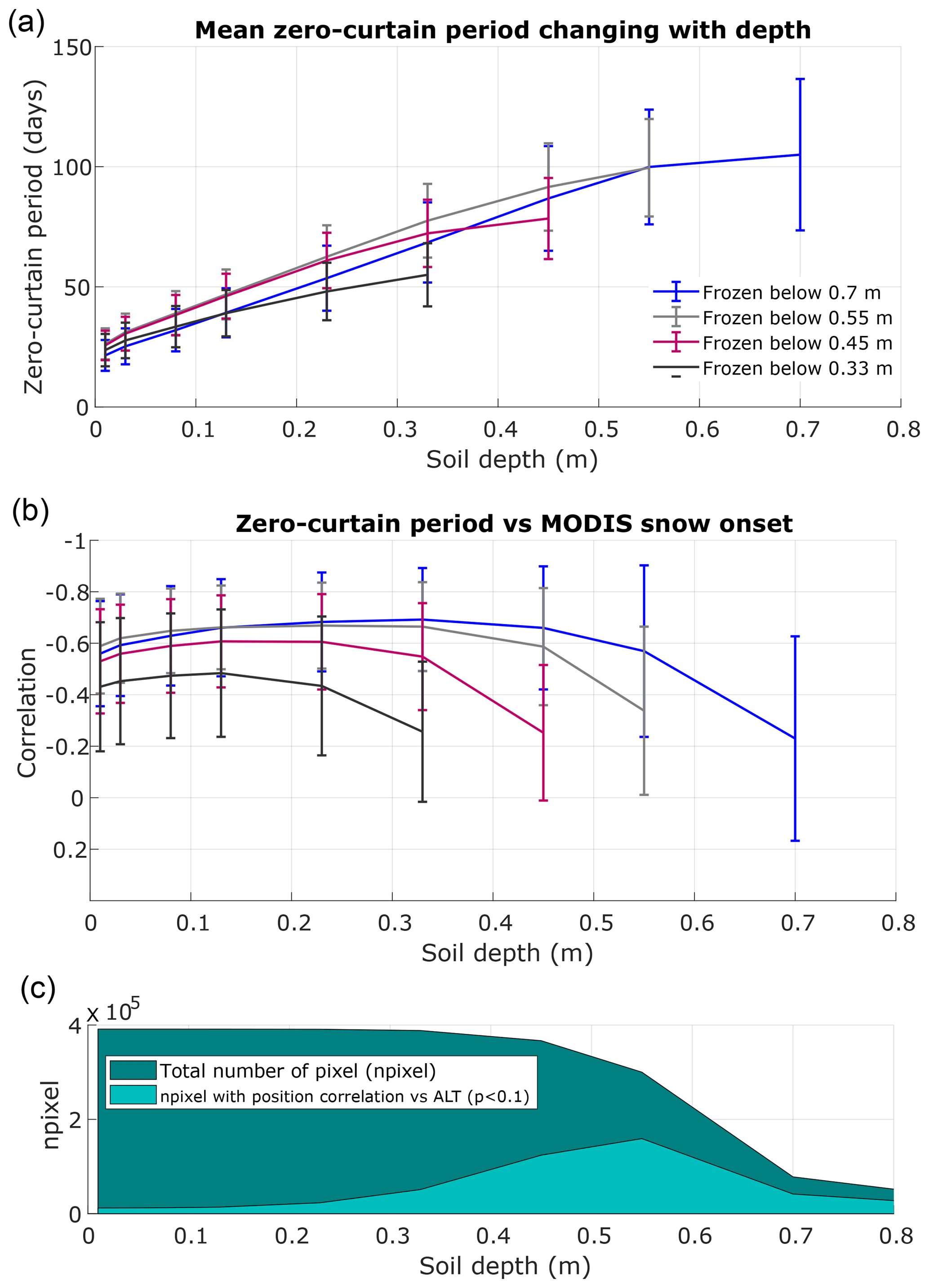
Figure 10Regional statistics of model-simulated zero-curtain period (a) and its sensitivity to MODIS snow onset and model-simulated ALT (b–c) from 2001 to 2016: (a) regional mean of model-simulated zero-curtain period at different depths; (b) changes in correlations between snow onset and zero-curtain period with depths; for both (a) and (b), the study area was divided into four groups: soil column froze below 0.33, 0.45, 0.55 and 0.7 m. The soil column for the majority of the study area froze below 0.7 m. (c) The proportion of pixels with a significant positive correlation between the zero-curtain period and ALT at different depths. The total number of unfrozen pixel was shown as “npixel”.
During the study period, the spatial pattern of model-simulated soil freeze onset and zero-curtain period trends at 0.25 and 0.35 m is closely associated with the trends of MODIS snow onset (Fig. 9); areas with earlier snow onset generally show later freeze onset and a longer zero-curtain period. Further analysis indicates that early snow accumulation is the main control on the soil freezing for the upper ( m) active-layer, while the zero-curtain period of deeper soils is more related to ALT (Fig. 10). The model simulations show an overall longer zero-curtain period in areas with deeper ALT. Approximately 55 % of the Arctic Alaska has a maximum thaw depth between 0.45 and 0.55 m. In those areas, correlations between MODIS snow onset and zero-curtain period generally decrease with increasing soil depths below 0.4 m, which corresponds to an increasing positive correlation between the ALT and zero-curtain period. This reduction of the correlation between snow onset and zero-curtain period is more pronounced in areas with shallower ALT. Compared with the zero-curtain period, we found a much weaker correlation between model-simulated soil freeze onset in near-surface soils (<0.1 m) and MODIS snow onset but similar relationships for soil depths below (>0.2 m) (Fig. S10). This is due to a positive correlation between surface freeze onset derived from MODIS LST and MODIS snow onset (R=0.71, p<0.1) in Arctic Alaska during the study period; earlier surface freezing leads to cold underlying soil, while earlier snow onset generally leads to warm soil in this area. Therefore, soil freeze onset for near-surface soils has weaker correlations with MODIS snow onset compared with the middle of the active layer (∼0.2–0.4 m), while the soil freeze onset is subject to similar controls as the zero-curtain period with soil depth increases. These results indicate that the land-surface temperature or F–T status may be a relatively poor indicator of soil-freezing status and the zero curtain period in the deeper active layer for the Arctic region.
4.1 Sensitivity of active-layer freezing process to recent climate change
Our results show a strong correlation between the active-layer freezing process and snow accumulation during the early snow season in Arctic Alaska, especially within upper ( m) soil layers. Earlier snow onset and establishment of a complete snow cover generally delays active-layer freezing and promotes a longer zero-curtain period (Figs. 8 and 9). Previous studies have highlighted the decoupling of surface air and soil temperatures during the winter season in the northern high latitudes due to strong insulating effects of snow cover (Morse et al., 2012; Throop et al., 2012; Koven et al., 2013; Smith et al., 2016). Changes in the rate of accumulation, timing, duration, density and amount of snow cover play an important role in determining how soil F–T dynamics respond to surface warming (Zhang, 2005; Lawrence and Slater, 2010). The relationship between fall snow onset and soil warming may vary depending on the timing and magnitude of snowfall, and local climate conditions (Yi et al., 2015). Early snow onset may enhance thermal buffering of cold surface temperatures and promote soil warming in colder climate zones such as Arctic Alaska. A shorter snow season may cool the soil in colder areas due to less insulation from cold atmospheric temperatures but may warm the soil in warmer areas by promoting greater heat transfer into soils (Lawrence and Slater, 2010). The snow cover impact on soil F–T dynamics will also depend on differences between the timing of first surface freeze and snow cover establishment, especially for near-surface ( m) soils (Kim et al., 2015).
Our model simulations also show that the influence of snow cover on soil freezing is weaker for deeper soil layers ( m), where the freeze onset and zero-curtain period are more closely related to the summer maximum thaw depth (i.e., ALT, Figs. 10 and S10). This can be largely explained by a close link between ALT and the soil-freezing lag rate of deeper soils. During fall, active-layer freezing proceeds both downward from the surface and upward from the underlying permafrost table (Outcalt et al., 1990; Oechel et al., 1997; Zona et al., 2016). This can be seen from the negative soil-freezing lag rate (related to differences in soil freeze onset between two adjacent soil layers) at the bottom of the active layer at the GTN-P sites (Fig. 6c–d), indicating that the bottom of the active layer freezes first. Increases in ALT can lead to abrupt changes in the soil-freezing lag rate at the same soil depth, which can change from a negative value to a small positive value and result in abrupt changes in the zero-curtain period at the bottom active layer (e.g., at the WD1 and WDN sites in Fig. S8b). Previous studies have also reported a delayed soil freeze-up and thus longer zero curtain with increasing ALT (Morse et al., 2012; Euskirchen et al., 2017). Based on the GTN-P site measurements, deeper soils show a general delay in soil freeze onset relative to shallower active layer, with a mean lag rate of 0.79±0.52 days cm−1 at 0.35 m depth; large variability in the soil-freezing lag rate is likely associated with different soil structure and variable active-layer soil moisture content (Throop et al., 2012). Therefore, a deepening active layer associated with climate warming will likely lead to a longer zero-curtain period in deeper soils.
The Arctic is expected to experience continued warming and precipitation increases under projected climate trends (IPCC, 2013), though the potential response of active-layer freezing to these changes may vary depending on changes in seasonal snow cover. Both surface warming and a changing precipitation regime can modify seasonal snow cover, leading to a nonlinear response of soil temperatures to warming (Lawrence and Slater, 2010; Yi et al., 2015). Increases in winter precipitation and snowpack deepening may enhance soil warming, while a reduced snowpack may promote soil cooling in colder climate areas. More frequent and intense rain-on-snow events during fall and early winter have been observed across the ABZ with recent warming trends (Ye et al., 2008; Langlois et al., 2017). Therefore, how these climate trends will affect soil moisture and thermal dynamics is a key challenge for accurately estimating soil F–T dynamics and potential carbon and climate feedbacks. In addition, with continued warming and ALT deepening, unfrozen conditions may persist in the bottom of the active layer, resulting in a perennially thawed subsurface soil layer or talik zone; once a talik forms, it can greatly accelerate permafrost degradation and result in large changes in surface hydrology and soil carbon decomposition (Yoshikawa and Hinzman, 2003; Parazoo et al., 2018).
Our model simulations are associated with large uncertainties, particularly regarding soil moisture effects on soil heat transfer during the F–T period. Changes in liquid water content during soil freezing vary for different soil conditions, while accurate simulation of this process is challenging due to complex processes controlling ice formation, liquid water movement and heat transfer in frozen soils (Outcalt et al., 1990; Romanovsky and Osterkamp, 2000; Schaefer and Jafarov, 2016). Our study used in situ soil dielectric constant (ε) measurements to parameterize the unfrozen water curve and determine the temperature threshold used to define soil freeze onset and calculate the zero-curtain period. However, our results also show large ε variability in response to freezing temperatures from the in situ SoilSCAPE measurements; the relationship between ε and liquid water content in organic-rich soils may also be different from mineral soils (Engstrom et al., 2005; Mironov et al., 2010). A reliable soil dielectric model characterizing the relations between unfrozen water content and ε for organic soils will help reduce the uncertainty in the estimated temperature threshold at soil freeze onset; a model sensitivity analysis using different b values in the unfrozen water curve (Eq. 11) may also help quantify uncertainties in the model-simulated zero-curtain period and its regional pattern. On the other hand, potential soil moisture redistribution with active-layer deepening is not accounted for in the current model, though this effect is likely small due to small ALT trends in this area during the study period (Yi et al., 2018). Increasing disturbance from thermokarst and wildfire are expected to alter microclimate and soil moisture conditions, vegetation cover and SOC stocks in the ABZ, which will also likely influence the dynamics of ground-ice evolution and permafrost degradation (Grosse et al., 2011; Liljedahl et al., 2016).
4.2 Potential use of remote-sensing to improve regional monitoring of soil F–T process
Large-scale satellite observations and global reanalysis data generally have difficulty capturing finer-scale snow cover variations and associated impacts on soil F–T dynamics. These limitations are exacerbated in the Arctic due to a paucity of regional climate stations and complex microclimate and snow cover conditions influenced by local topography, vegetation and winds (Liston and Sturm, 2002; Gisnås et al., 2016). Optical satellite remote sensing, including Landsat and MODIS sensors, can provide accurate local-scale information on the snow cover extent, though effective regional monitoring from these observations is constrained by persistent cloud cover and reduced solar illumination for much of the year. Moreover, these observations do not include snow depth or water content information, which are critical parameters for hydrologic and ecological applications (Brown et al., 2010; Painter et al., 2016). Snow-covered areas attenuate the emitted microwave radiation from the underlying surface, while the magnitude of microwave emissions and attenuation depends on the sensor frequency, snow liquid water content, snow grain size and shape. Thus, snow properties, including snow water equivalent (SWE), may be derived from passive microwave sensors, albeit at relatively coarse spatial scale (Kelly et al., 2003; Armstrong et al., 2005; Takala et al., 2011). However, its accuracy is limited in deep snowpack conditions, and its applicability is limited in forest areas and wet snow conditions (Frei et al., 2012). Compared with passive microwave sensors, active radars or scatterometers such as Ku band are capable of much higher spatial resolutions and can be particularly useful for regional snow mapping (Yueh et al., 2009). However, more studies are needed to clarify the multiple scattering effects from snow microstructure variations and contributions from other elements within the sensor footprint including vegetation, soil and open-water effects, to ensure accurate retrieval of snow properties (King et al., 2018). Airborne laser altimeters (lidar) also show strong potential for mapping snow depth patterns (Deems et al., 2013; Painter et al., 2016), while the recently launched ICESat-2 is expected to provide new capabilities of satellite lidar for regional snow mapping (Kwok and Markus, 2018). In the near term, significant improvements in acquiring geospatial information on snow properties in the Arctic will likely come from merging in situ and modeling data sets with multi-sensor snow products (Painter et al., 2016).
Another major challenge for regional permafrost modeling is the lack of information on subsurface properties, particularly for organic soils with distinct hydraulic and thermal properties. Current permafrost models generally use regional or global SOC inventory data to parameterize the SOC profile following an exponentially decreasing curve (Lawrence and Slater, 2008; Rawlins et al., 2013; Yi et al., 2018). However, large discrepancies are apparent from the available SOC inventory records in the ABZ (Liu et al., 2013; Hugelius et al., 2014). There is also large regional variability in the vertical SOC distribution due to multiple processes affecting the SOC distribution in cryoturbated soils (Mishra et al., 2013; Hugelius et al., 2014; Hossain et al., 2015). Long wavelength radar, including P-band (∼70 cm) and L-band (∼24 cm), is sensitive to surface vegetation structure, soil surface and subsurface dielectric properties (e.g., Dobson et al., 1985; Mironov et al., 2010; Tabatabaeenejad et al., 2015). Our model experiments and analysis using in situ dielectric constant measurements and a P-band radar-retrieved soil dielectric constant for soil-freezing studies, albeit simple, show the potential of longwave radar remote sensing in mapping of SOC, active layer F–T and moisture profiles. However, similarly to many other inversion problems, radar retrievals suffer from ambiguity in the inversion parameter definitions, mainly due to insufficient information on the subsurface profile (e.g., Tabatabaeenejad et al., 2015; Chen et al., 2019). Therefore, new methodologies are needed to address the underdetermined nature of the radar backscatter inversion and associated land parameter retrievals, by either including additional observations or other synergistic information from soil physical models to reduce parameter dimensions in the radar model (e.g., Sadeghi et al., 2016). The vegetation canopy also has a large impact on the radar backscatter, especially at L-band and shorter wavelengths, while separating the radar contribution of subsurface soils from the vegetation canopy remains a challenge. Radar measurements with shorter wavelengths (e.g., X, C, L-bands) can be also useful for subsurface retrievals by providing contributing information on surface snow, soil and vegetation conditions (Moghaddam et al., 2000; Yueh et al., 2009; King et al., 2018), which can be used to reduce the uncertainties in the longwave (e.g., P-band) radar soil parameter retrievals. However, more sophisticated modeling experiments capable of representing complex landscapes and multi-frequency radar backscatter characteristics are needed to fully clarify the value of multi-frequency observations. Additional airborne radar sampling targeting regional disturbance gradients may also provide the necessary information for the regional modeling framework to represent increasing disturbance regimes and associated impacts on active-layer F–T dynamics in the ABZ.
In this study, we used a remote-sensing-driven permafrost model and a newly developed fine-resolution snow data set to simulate the active-layer freezing process, including soil freeze onset and zero-curtain period in Arctic Alaska during the recent satellite period (2001–2016). The model simulations were combined with multiple in situ measurements and local-scale soil dielectric constant retrievals derived from airborne longwave (P-band) radar data to investigate the regional sensitivity of soil freezing and zero-curtain period to recent climate change. Our results indicate that (1) the soil freeze onset and zero-curtain period in the upper soils (<0.4 m) are primarily affected by snow accumulation during the early cold season, whereby areas with earlier snow onset generally show a delayed soil freeze onset and prolonged zero-curtain period; (2) the influence of snow onset and accumulation on the soil freezing decreases with increasing soil depth and the zero-curtain period of deeper soils (>0.5 m) are more closely related to ALT due to an increasing delay in soil freezing with active-layer deepening. Therefore, a deepening active layer associated with climate warming will very likely lead to a longer unfrozen period in deeper soils and potentially result in more cold-season carbon loss. These findings highlight the importance of relatively fine-scale snow cover and active-layer thickness products for a better understanding of potential carbon and climate feedbacks in permafrost ecosystems. Our model experiments and analysis, using in situ and radar-retrieved dielectric constant data to characterize soil freezing, show the potential of longwave radar remote sensing for landscape-level mapping of active-layer soil properties, including SOC, F–T and soil moisture profiles. Future satellite P- and L-band radar missions including NISAR, Tandem-L and BIOMASS (Arcioni et al., 2014; Moreira et al., 2015; Rosen et al., 2017) may enable substantial improvements in the way models represent fine-scale soil processes and thus allow for more accurate predictions of boreal and Arctic environmental changes.
The regional model simulations will be archived and distributed for public access through NASA ABoVE archive at the NASA ORNL DAAC. Radar retrievals are available upon request, and other data used in this study were obtained from free and open data repositories. Code for snow data processing and permafrost modeling is also available upon request.
The supplement related to this article is available online at: https://doi.org/10.5194/tc-13-197-2019-supplement.
YY and CEM initiated the study. YY did the calculations and wrote the paper. RHC and MM contributed to the data. All authors contributed to the discussions and provided feedback on the final version.
The authors declare that they have no conflict of interest.
Funding for this study was provided by NASA (NNX15AT74A, NNX14AO23G). The
authors thank Vladimir Romanovsky's group for providing the GTN-P soil temperature
data in Alaska. A portion of this research was carried out at the Jet
Propulsion Laboratory, California Institute of Technology, under contract
with NASA.
Edited by: Chris Derksen
Reviewed by: two anonymous referees
Arcioni, M., Bensi, P., Fehringer, M., Fois, F., Heliere, F., Lin, C.-C., and Scipal, K.: The Biomass mission, status of the satellite system, 2014 IEEE Geoscience and Remote Sensing Symposium, Quebec City, QC, 1413–1416, https://doi.org/10.1109/IGARSS.2014.6946700, 2014.
Armstrong, R., Brodzik, M. J., Knowles, K., and Savoie, M.: Global Monthly EASE-Grid Snow Water Equivalent Climatology, Version 1, Indicate subset used, Boulder, Colorado USA, NASA National Snow and Ice Data Center, Distributed Active Archive Center, https://doi.org/10.5067/KJVERY3MIBPS, 2005.
Banin, A. and Anderson, D. M.: Effects of Salt Concentration Changes During Freezing on the Unfrozen Water Content of Porous Materials, Water Resour. Res., 10, 124–128, https://doi.org/10.1029/WR010i001p00124, 1974.
Biskaborn, B. K., Lanckman, J.-P., Lantuit, H., Elger, K., Streletskiy, D. A., Cable, W. L., and Romanovsky, V. E.: The new database of the Global Terrestrial Network for Permafrost (GTN-P), Earth Syst. Sci. Data, 7, 245–259, https://doi.org/10.5194/essd-7-245-2015, 2015.
Brown, J., Hinkel, K. M., and Nelson, F. E.: The circumpolar active layer monitoring (CALM) program: Research designs and initial results, Polar Geography, 24, 166–258, 2000.
Brown, R., Derksen, C., and Wang, L.: A multi-data set analysis of variability and change in Arctic spring snow cover extent, 1967–2008, J. Geophys. Res., 115, D16111, https://doi.org/10.1029/2010JD013975, 2010.
Brown, R. D. and Derksen, C.: Is Eurasian October snow cover extent increasing?, Environ. Res. Lett., 8, 024006, https://doi.org/10.1088/1748-9326/8/2/024006, 2013.
Burke, E. J., Dankers, R., Jones, C. D., and Wiltshire, A. J.: A retrospective analysis of pan Arctic permafrost using the JULES land surface model, Clim. Dynam., 41, 1025–1038, https://doi.org/10.1007/s00382-012-1648-x, 2013.
Calonne, N., Flin, F., Morin, S., Lesaffre, B., du Roscoat, S. R., and Geindreau, C.: Numerical and experimental investigations of the effective thermal conductivity of snow, Geophys. Res. Lett., 38, L23501, https://doi.org/10.1029/2011GL049234, 2011.
Chen, R. H., Tabatabaeenejad, A., and Moghaddam, M.: P-Band Radar Retrieval of Permafrost Active Layer Properties: Time-Series Approach and Validation with in-situ Observations IEEE International Geoscience and Remote Sensing Symposium (IGARSS), Valencia, 6777–6779, https://doi.org/10.1109/IGARSS.2018.8518179, 2018.
Chen, R. H., Tabatabaeenejad, A., and Moghaddam, M.: Retrieval of Permafrost Active Layer Properties Using Time-Series P-Band Radar Observations, IEEE T. Geosci. Remote, accepted, 2019.
Commane, R., Lindaas, J., Benmergui, J., Luus, K. A., Chang, R. Y.-W., Daube, B. C., Euskirchen, E. S., Henderson, J. M., Karion, A., Miller, J. B., Miller, S. M., Parazoo, N. C., Randerson, J. T., Sweeney, C., Tans, P., Thoning, K., Veraverbeke, S., Miller, C. E. and Wofsy, S. C.: Carbon dioxide sources from Alaska driven by increasing early winter respiration from Arctic tundra, P. Natl. Acad. Sci. USA, https://doi.org/10.1073/pnas.1618567114, 2017.
Deems, J. S., Painter, T. H., and Finnegan, D. C.: Lidar measurement of snow depth: a review, J. Glaciol., 59, 467–479, https://doi.org/10.3189/2013JoG12J154, 2013.
De Lannoy, G. J. M., Koster, R. D., Reichle, R. H., Mahanama, S. P. P., and Liu, Q.: An updated treatment of soil texture and associated hydraulic properties in a global land modeling system, J. Adv. Model. Earth Sy., 6, 957–979, 2014.
Derksen, C., Xu, X., Scott Dunbar, R., Colliander, A., Kim, Y., Kimball, J. S., Black, T. A., Euskirchen, E., Langlois, A., Loranty, M. M., Marsh, P., Rautiainen, K., Roy, A., Royer, A., and Stephens, J.: Retrieving landscape freeze/thaw state from Soil Moisture Active Passive (SMAP) radar and radiometer measurements, Remote Sens. Environ., 194, 48–62, https://doi.org/10.1016/j.rse.2017.03.007, 2017.
Dobson, M., Ulaby, F., Hallikainen, M., and El-rayes, M.: Microwave Dielectric Behavior of Wet Soil-Part II: Dielectric Mixing Models, IEEE T. Geosci. Remote, GE-23, 35–46, https://doi.org/10.1109/TGRS.1985.289498, 1985.
Engstrom, R., Hope, A., Kwon, H., Stow, D., and Zamolodchikov, D.: Spatial distribution of near surface soil moisture and its relationship to microtopography in the Alaskan Arctic coastal plain, Hydrol. Res., 36, 219–234, https://doi.org/10.2166/nh.2005.0016, 2005.
Euskirchen, E. S., Bret-Harte, M. S., Shaver, G. R., Edgar, C. W., and Romanovsky, V. E.: Long-Term Release of Carbon Dioxide from Arctic Tundra Ecosystems in Alaska, Ecosystems, 20, 960–974, https://doi.org/10.1007/s10021-016-0085-9, 2017.
Farouki, O. T.: Thermal properties of soils, Report No. 81, CRREL Monograph, United States Army Corps of Engineers Cold Regions Research and Engineering Laboratory, Hanover, New Hampshire, USA, 1981.
Frei, A., Tedesco, M., Lee, S., Foster, J., Hall, D. K., Kelly, R., and Robinson, D. A.: A review of global satellite-derived snow products, Adv. Space Res., 50, 1007–1029, https://doi.org/10.1016/j.asr.2011.12.021, 2012.
Gafurov, A. and Bárdossy, A.: Cloud removal methodology from MODIS snow cover product, Hydrol. Earth Syst. Sci., 13, 1361–1373, https://doi.org/10.5194/hess-13-1361-2009, 2009.
Gelaro, R., McCarty, W., Suárez, M. J., Todling, R., Molod, A., Takacs, L., Randles, C. A., Darmenov, A., Bosilovich, M. G., Reichle, R., Wargan, K., Coy, L., Cullather, R., Draper, C., Akella, S., Buchard, V., Conaty, A., da Silva, A. M., Gu, W., Kim, G.-K., Koster, R., Lucchesi, R., Merkova, D., Nielsen, J. E., Partyka, G., Pawson, S., Putman, W., Rienecker, M., Schubert, S. D., Sienkiewicz, M., and Zhao, B.: The Modern-Era Retrospective Analysis for Research and Applications, Version 2 (MERRA-2), J. Climate, 30, 5419–5454, 2017.
Gisnås, K., Westermann, S., Schuler, T. V., Melvold, K., and Etzelmüller, B.: Small-scale variation of snow in a regional permafrost model, The Cryosphere, 10, 1201–1215, https://doi.org/10.5194/tc-10-1201-2016, 2016.
Grosse, G., Harden, J., Turetsky, M., McGuire, A. D., Camill, P., Tarnocai, C., Frolking, S., Schuur, E. A. G., Jorgenson, T., Marchenko, S., Romanovsky, V., Wickland, K. P., French, N., Waldrop, M., Bourgeau-Chavez, L., and Striegl, R. G.: Vulnerability of high-latitude soil organic carbon in North America to disturbance, J. Geophys. Res.-Biogeo., 116, G00K06, 2011.
Grünewald, T., Bühler, Y., and Lehning, M.: Elevation dependency of mountain snow depth, The Cryosphere, 8, 2381–2394, https://doi.org/10.5194/tc-8-2381-2014, 2014.
Hall, D. K. and Riggs, G. A.: MODIS/Terra Snow Cover 8-Day L3 Global 500 m Grid, Version 6, NASA National Snow and Ice Data Center Distributed Active Archive Center, Boulder, Colorado, USA, https://doi.org/10.5067/MODIS/MOD10A2.006, 2016.
Henn, B., Newman, A. J., Livneh, B., Daly, C., and Lundquist, J. D.: An assessment of differences in gridded precipitation datasets in complex terrain, J. Hydrol., 556, 1205–1219, https://doi.org/10.1016/j.jhydrol.2017.03.008, 2018.
Hossain, M. F., Chen, W., and Zhang, Y.: Bulk density of mineral and organic soils in the Canada's arctic and sub-arctic, Information Processing in Agriculture, 2, 183–190, 2015.
Hugelius, G., Strauss, J., Zubrzycki, S., Harden, J. W., Schuur, E. A. G., Ping, C.-L., Schirrmeister, L., Grosse, G., Michaelson, G. J., Koven, C. D., O'Donnell, J. A., Elberling, B., Mishra, U., Camill, P., Yu, Z., Palmtag, J., and Kuhry, P.: Estimated stocks of circumpolar permafrost carbon with quantified uncertainty ranges and identified data gaps, Biogeosciences, 11, 6573–6593, https://doi.org/10.5194/bg-11-6573-2014, 2014.
IPCC: Climate Change 2013: The Physical Science Basis, Cambridge University Press, Cambridge, United Kingdom and New York, NY, USA, 1535 pp., https://doi.org/10.1017/CBO9781107415324, 2013.
Jafarov, E. E., Coon, E. T., Harp, D. R., Wilson, C. J., Painter, S. L., Atchley, A. L., and Romanovsky, V. E.: Modeling the role of preferential snow accumulation in through talik development and hillslope groundwater flow in a transitional permafrost landscape, Environ. Res. Lett., 13, 105006, https://doi.org/10.1088/1748-9326/aadd30, 2018.
Jin, S. M., Yang, L. M., Danielson, P., Homer, C., Fry, J., and Xian, G.: A comprehensive change detection method for updating the National Land Cover Database to circa 2011, Remote Sens. Environ., 132, 159–175, 2013.
Kelly, R. E., Chang, A. T., Tsang, L., and Foster, J. L.: A prototype AMSR-E global snow area and snow depth algorithm, IEEE T. Geosci. Remote, 41, 230–242, https://doi.org/10.1109/TGRS.2003.809118, 2003.
Kim, Y., Kimball, J. S., Robinson, D. A., and Derksen, C.: New satellite climate data records indicate strong coupling between recent frozen season changes and snow cover over high northern latitudes, Environ. Res. Lett., 10, 084004, https://doi.org/10.1088/1748-9326/10/8/084004, 2015.
King, J., Derksen, C., Toose, P., Langlois, A., Larsen, C., Lemmetyinen, J., Marsh, P., Montpetit, B., Roy, A., Rutter, N., and Sturm, M.: The influence of snow microstructure on dual-frequency radar measurements in a tundra environment, Remote Sens. Environ., 215, 242–254, https://doi.org/10.1016/j.rse.2018.05.028, 2018.
Kirchner, P. B., Bales, R. C., Molotch, N. P., Flanagan, J., and Guo, Q.: LiDAR measurement of seasonal snow accumulation along an elevation gradient in the southern Sierra Nevada, California, Hydrol. Earth Syst. Sci., 18, 4261–4275, https://doi.org/10.5194/hess-18-4261-2014, 2014.
Kittler, F., Heimann, M., Kolle, O., Zimov, N., Zimov, S., and Göckede, M.: Long-Term Drainage Reduces CO2 Uptake and CH4 Emissions in a Siberian Permafrost Ecosystem: Drainage impact on Arctic carbon cycle, Global Biogeochem. Cy., 31, 1704–1717, https://doi.org/10.1002/2017GB005774, 2017.
Koven, C. D., Riley, W. J., and Stern, A.: Analysis of permafrost thermal dynamics and response to climate change in the CMIP5 Earth System Models, J. Climate, 26, 1877–1900, 2013.
Kwok, R. and Markus, T.: Potential basin-scale estimates of Arctic snow depth with sea ice freeboards from CryoSat-2 and ICESat-2: An exploratory analysis, Adv. Space Res., 62, 1243–1250, https://doi.org/10.1016/j.asr.2017.09.007, 2018.
Langlois, A., Johnson, C.-A., Montpetit, B., Royer, A., Blukacz-Richards, E. A., Neave, E., Dolant, C., Roy, A., Arhonditsis, G., Kim, D.-K., Kaluskar, S., and Brucker, L.: Detection of rain-on-snow (ROS) events and ice layer formation using passive microwave radiometry: A context for Peary caribou habitat in the Canadian Arctic, Remote Sens. Environ., 189, 84–95, https://doi.org/10.1016/j.rse.2016.11.006, 2017.
Lawrence, D. M. and Slater, A. G.: Incorporating organic soil into a global climate model, Clim. Dynam., 30, 145–160, 2008.
Lawrence, D. M. and Slater, A. G.: The contribution of snow condition trends to future ground climate, Clim. Dynam., 34, 969–981, 2010.
Lawrence, D. M., Koven, C. D., Swenson, S. C., Riley, W. J., and Slater, A. G.: Permafrost thaw and resulting soil moisture changes regulate projected high-latitude CO 2 and CH 4 emissions, Environ. Res. Lett., 10, 094011, https://doi.org/10.1088/1748-9326/10/9/094011, 2015.
Letts, M. G., Roulet, N. T., Comer, N. T., Skarupa, M. R., and Verseghy, D. L.: Parametrization of peatland hydraulic properties for the Canadian land surface scheme, Atmosphere-Ocean, 38, 141–160, https://doi.org/10.1080/07055900.2000.9649643, 2000.
Liljedahl, A. K., Boike, J., Daanen, R. P., Fedorov, A. N., Frost, G. V., Grosse, G., Hinzman, L. D., Iijma, Y., Jorgenson, J. C., Matveyeva, N., Necsoiu, M., Raynolds, M. K., Romanovsky, V. E., Schulla, J., Tape, K. D., Walker, D. A., Wilson, C. J., Yabuki, H., and Zona, D.: Pan-Arctic ice-wedge degradation in warming permafrost and its influence on tundra hydrology, Nat. Geosci., 9, 312–319, 2016.
Liston, G. E. and Sturm, M.: Winter Precipitation Patterns in Arctic Alaska Determined from a Blowing-Snow Model and Snow-Depth Observations, J. Hydrometeorol., 3, 646–659, https://doi.org/10.1175/1525-7541(2002)003<0646:WPPIAA>2.0.CO;2, 2002.
Liu, S., Wei, Y., Post, W. M., Cook, R. B., Schaefer, K., and Thornton, M. M.: The Unified North American Soil Map and its implication on the soil organic carbon stock in North America, Biogeosciences, 10, 2915–2930, https://doi.org/10.5194/bg-10-2915-2013, 2013.
Mironov, V. L., De Roo, R. D., and Savin, I. V.: Temperature-Dependable Microwave Dielectric Model for an Arctic Soil, IEEE T. Geosci. Remote, 48, 2544–2556, https://doi.org/10.1109/TGRS.2010.2040034, 2010.
Mishra, U., Jastrow, J. D., Matamala, R., Hugelius, G., Koven, C. D., Harden, J. W., Ping, C. L., Michaelson, G. J., Fan, Z., Miller, R. M., McGuire, A. D., Tarnocai, C., Kuhry, P., Riley, W. J., Schaefer, K., Schuur, E. A. G., Jorgenson, M. T., and Hinzman, L. D.: Empirical estimates to reduce modeling uncertainties of soil organic carbon in permafrost regions: a review of recent progress and remaining challenges, Environ. Res. Lett., 8, 035020, 2013.
Mishra, U., Drewniak, B., Jastrow, J. D., Matamala, R. M., and Vitharana, U. W. A.: Spatial representation of organic carbon and active-layer thickness of high latitude soils in CMIP5 earth system models, Geoderma, 300, 55–63, 2016.
Moghaddam, M., Saatchi, S., and Cuenca, R. H.: Estimating subcanopy soil moisture with radar, J. Geophys. Res.-Atmos., 105, 14899–14911, https://doi.org/10.1029/2000JD900058, 2000.
Moghaddam, M., Entekhabi, D., Goykhman, Y., Li, K., Liu, M., Mahajan, A., Nayyar, A., Shuman, D., and Teneketzis, D.: A Wireless Soil Moisture Smart Sensor Web Using Physics-Based Optimal Control: Concept and Initial Demonstrations, IEEE J. Sel. Top. Appl., 3, 522–535, https://doi.org/10.1109/JSTARS.2010.2052918, 2010.
Moreira, A., Krieger, G., Hajnsek, I., Papathanassiou, K., Younis, M., Lopez-Dekker, P., Huber, S., Villano, M., Pardini, M., Eineder, M., De Zan, F., and Parizzi, A.: Tandem-L: A Highly Innovative Bistatic SAR Mission for Global Observation of Dynamic Processes on the Earth's Surface, IEEE Geosci. Remote Sens. Mag., 3, 8–23, https://doi.org/10.1109/MGRS.2015.2437353, 2015.
Morse, P. D., Burn, C. R., and Kokelj, S. V.: Influence of snow on near-surface ground temperatures in upland and alluvial environments of the outer Mackenzie Delta, Northwest Territories, edited by: Allard, M., Can. J. Earth Sci., 49, 895–913, https://doi.org/10.1139/e2012-012, 2012.
Naeimi, V., Paulik, C., Bartsch, A., Wagner, W., Kidd, R., Park, S.-E., Elger, K., and Boike, J.: ASCAT Surface State Flag (SSF): Extracting Information on Surface Freeze/Thaw Conditions From Backscatter Data Using an Empirical Threshold-Analysis Algorithm, IEEE T. Geosci. Remote, 50, 2566–2582, https://doi.org/10.1109/TGRS.2011.2177667, 2012.
Nicolsky, D. J., Romanovsky, V. E., Alexeev, V. A., and Lawrence, D. M.: Improved modeling of permafrost dynamics in a GCM land-surface scheme, Geophys. Res. Lett., 34, L08501, https://doi.org/10.1029/2007GL029525, 2007.
Oechel, W. C., Vourlitis, G., and Hastings, S. J.: Cold season CO2 emission from arctic soils, Global Biogeochem. Cy., 11, 163–172, 1997.
Outcalt, S. I., Nelson, F. E., and Hinkel, K. M.: The zero-curtain effect: Heat and mass transfer across an isothermal region in freezing soil, Water Resour. Res., 26, 1509–1516, https://doi.org/10.1029/WR026i007p01509, 1990.
Painter, T. H., Berisford, D. F., Boardman, J. W., Bormann, K. J., Deems, J. S., Gehrke, F., Hedrick, A., Joyce, M., Laidlaw, R., Marks, D., Mattmann, C., McGurk, B., Ramirez, P., Richardson, M., Skiles, S. M., Seidel, F. C., and Winstral, A.: The Airborne Snow Observatory: Fusion of scanning lidar, imaging spectrometer, and physically-based modeling for mapping snow water equivalent and snow albedo, Remote Sens. Environ., 184, 139–152, https://doi.org/10.1016/j.rse.2016.06.018, 2016.
Paquin, J.-P. and Sushama, L.: On the Arctic near-surface permafrost and climate sensitivities to soil and snow model formulations in climate models, Clim. Dynam., 44, 203–228, https://doi.org/10.1007/s00382-014-2185-6, 2015.
Parajka, J. and Blöschl, G.: Spatio-temporal combination of MODIS images – potential for snow cover mapping: SPATIO-TEMPORAL COMBINATION OF MODIS IMAGES, Water Resour. Res., 44, W03406, https://doi.org/10.1029/2007WR006204, 2008.
Parajka, J., Pepe, M., Rampini, A., Rossi, S., and Blöschl, G.: A regional snow-line method for estimating snow cover from MODIS during cloud cover, J. Hydrol., 381, 203–212, https://doi.org/10.1016/j.jhydrol.2009.11.042, 2010.
Parazoo, N. C., Koven, C. D., Lawrence, D. M., Romanovsky, V., and Miller, C. E.: Detecting the permafrost carbon feedback: talik formation and increased cold-season respiration as precursors to sink-to-source transitions, The Cryosphere, 12, 123–144, https://doi.org/10.5194/tc-12-123-2018, 2018.
Park, C.-H., Behrendt, A., LeDrew, E., and Wulfmeyer, V.: New Approach for Calculating the Effective Dielectric Constant of the Moist Soil for Microwaves, Remote Sens., 9, 732, https://doi.org/10.3390/rs9070732, 2017.
Pastick, N. J., Jorgenson, M. T., Wylie, B. K., Nield, S. J., Johnson, K. D., and Finley, A. O.: Distribution of near-surface permafrost in Alaska: Estimates of present and future conditions, Remote Sens. Environ., 168, 301–315, 2015.
Qian, B., Gregorich, E. G., Gameda, S., Hopkins, D. W., and Wang, X. L.: Observed soil temperature trends associated with climate change in Canada, J. Geophys. Res., 116, D02106, https://doi.org/10.1029/2010JD015012, 2011.
Rawlins, M. A., Nicolsky, D. J., McDonald, K. C., and Romanovsky, V. E.: Simulating soil freeze/thaw dynamics with an improved pan-Arctic water balance model, J. Adv. Model. Earth Sy., 5, 659–675, 2013.
Rautiainen, K., Parkkinen, T., Lemmetyinen, J., Schwank, M., Wiesmann, A., Ikonen, J., Derksen, C., Davydov, S., Davydova, A., Boike, J., Langer, M., Drusch, M., and Pulliainen, J.: SMOS prototype algorithm for detecting autumn soil freezing, Remote Sens. Environ., 180, 346–360, https://doi.org/10.1016/j.rse.2016.01.012, 2016.
Reichle, R. H., De Lannoy, G. J. M., Liu, Q., Ardizzone, J. V., Colliander, A., Conaty, A., Crow, W., Jackson, T. J., Jones, L. A., Kimball, J. S., Koster, R. D., Mahanama, S. P., Smith, E. B., Berg, A., Bircher, S., Bosch, D., Caldwell, T. G., Cosh, M., González-Zamora, Á., Holifield Collins, C. D., Jensen, K. H., Livingston, S., Lopez-Baeza, E., Martínez-Fernández, J., McNairn, H., Moghaddam, M., Pacheco, A., Pellarin, T., Prueger, J., Rowlandson, T., Seyfried, M., Starks, P., Su, Z., Thibeault, M., van der Velde, R., Walker, J., Wu, X., and Zeng, Y.: Assessment of the SMAP Level-4 Surface and Root-Zone Soil Moisture Product Using In Situ Measurements, J. Hydrometeorol., 18, 2621–2645, 2017.
Romanovsky, V. E. and Osterkamp, T. E.: Effects of unfrozen water on heat and mass transport processes in the active layer and permafrost, Permafrost Periglac., 11, 219–239, 2000.
Rosen, P., Hensley, S., Shaffer, S., Edelstein, W., Kim, Y., Kumar, R., Misra, T., Bhan, R., and Sagi, R.: The NASA-ISRO SAR (NISAR) mission dual-band radar instrument preliminary design, in: 2017 IEEE International Geoscience and Remote Sensing Symposium (IGARSS), 3832–3835, IEEE, Fort Worth, TX, 2017.
Sadeghi, M., Tabatabaeenejad, A., Tuller, M., Moghaddam, M., and Jones, S.: Advancing NASA's AirMOSS P-Band Radar Root Zone Soil Moisture Retrieval Algorithm via Incorporation of Richards' Equation, Remote Sens., 9, 17, https://doi.org/10.3390/rs9010017, 2016.
Schaefer, K. and Jafarov, E.: A parameterization of respiration in frozen soils based on substrate availability, Biogeosciences, 13, 1991–2001, https://doi.org/10.5194/bg-13-1991-2016, 2016.
Schaefer, G. L. and Paetzold, R. F.: SNOTEL (SNOwpack TELemetry) and SCAN (Soil Climate Analysis Network) presented at the Automated Weather Station (AWS) workshop, 6–10 March, Lincoln, NE, 2000.
Schuur, E. A. G., McGuire, A. D., Schadel, C., Grosse, G., Harden, J. W., Hayes, D. J., Hugelius, G., Koven, C. D., Kuhry, P., Lawrence, D. M., Natali, S. M., Olefeldt, D., Romanovsky, V. E., Schaefer, K., Turetsky, M. R., Treat, C. C., and Vonk, J. E.: Climate change and the permafrost carbon feedback, Nature, 520, 171–179, 2015.
Slater, A. G. and Lawrence, D. M.: Diagnosing Present and Future Permafrost from Climate Models, J. Climate, 26, 5608–5623, 2013.
Smith, S. L., Riseborough, D. W., Bonnaventure, P. P., and Duchesne, C.: An ecoregional assessment of freezing season air and ground surface temperature in the Mackenzie Valley corridor, NWT, Canada, Cold Reg. Sci. Technol., 125, 152–161, https://doi.org/10.1016/j.coldregions.2016.02.007, 2016.
Sturm, M., Taras, B., Liston, G. E., Derksen, C., Jonas, T., and Lea, J.: Estimating Snow Water Equivalent Using Snow Depth Data and Climate Classes, J. Hydrometeorol., 11, 1380–1394, 2010.
Tabatabaeenejad, A., Burgin, M., Duan, X. Y., and Moghaddam, M.: P-Band Radar Retrieval of Subsurface Soil Moisture Profile as a Second-Order Polynomial: First AirMOSS Results, IEEE T. Geosci. Remote, 53, 645–658, 2015.
Takala, M., Luojus, K., Pulliainen, J., Derksen, C., Lemmetyinen, J., Kärnä, J.-P., Koskinen, J., and Bojkov, B.: Estimating northern hemisphere snow water equivalent for climate research through assimilation of space-borne radiometer data and ground-based measurements, Remote Sens. Environ., 115, 3517–3529, https://doi.org/10.1016/j.rse.2011.08.014, 2011.
Thornton, P. E., Running, S. W., and White, M. A.: Generating surfaces of daily meteorological variables over large regions of complex terrain, J. Hydrol., 190, 214–251, https://doi.org/10.1016/S0022-1694(96)03128-9, 1997.
Throop, J., Lewkowicz, A. G., and Smith, S. L.: Climate and ground temperature relations at sites across the continuous and discontinuous permafrost zones, northern Canada, Can. J. Earth Sci., 49, 865–876, https://doi.org/10.1139/e11-075, 2012.
U.S. Geological Survey: Alaska 2 Arc-second Digital Elevation Models (DEMs) – USGS National Map 3DEP Downloadable Data Collection, U.S. Geological Survey, 2017.
Walvoord, M. A. and Kurylyk, B. L.: Hydrologic Impacts of Thawing Permafrost-A Review, Vadose Zone J., 15, vzj2016.01.0010, 2016.
Wan, Z. S. H. and Hulley, G.: MOD11A2 MODIS/Terra Land Surface Temperature/Emissivity 8-Day L3 Global 1 km SIN Grid V006, NASA EOSDIS Land Processes DAAC, https://doi.org/10.5067/MODIS/MOD11A2.006, 2015.
Westermann, S., Peter, M., Langer, M., Schwamborn, G., Schirrmeister, L., Etzelmüller, B., and Boike, J.: Transient modeling of the ground thermal conditions using satellite data in the Lena River delta, Siberia, The Cryosphere, 11, 1441–1463, https://doi.org/10.5194/tc-11-1441-2017, 2017.
Woo, M. K.: Permafrost hydrology, Springer-Verlag, Heidelberg, Germany, 575 pp., 2012.
Ye, H., Yang, D., and Robinson, D.: Winter rain on snow and its association with air temperature in northern Eurasia, Hydrol. Process., 22, 2728–2736, https://doi.org/10.1002/hyp.7094, 2008.
Yi, Y., Kimball, J. S., Rawlins, M. A., Moghaddam, M., and Euskirchen, E. S.: The role of snow cover affecting boreal-arctic soil freeze–thaw and carbon dynamics, Biogeosciences, 12, 5811–5829, https://doi.org/10.5194/bg-12-5811-2015, 2015.
Yi, Y., Kimball, J. S., Chen, R. H., Moghaddam, M., Reichle, R. H., Mishra, U., Zona, D., and Oechel, W. C.: Characterizing permafrost active layer dynamics and sensitivity to landscape spatial heterogeneity in Alaska, The Cryosphere, 12, 145–161, https://doi.org/10.5194/tc-12-145-2018, 2018.
Yoshikawa, K. and Hinzman, L. D.: Shrinking thermokarst ponds and groundwater dynamics in discontinuous permafrost near council, Alaska, Permafrost Periglac., 14, 151–160, https://doi.org/10.1002/ppp.451, 2003.
Yueh, S. H., Dinardo, S. J., Akgiray, A., West, R., Cline, D. W., and Elder, K.: Airborne Ku-Band Polarimetric Radar Remote Sensing of Terrestrial Snow Cover, IEEE T. Geosci. Remote, 47, 3347–3364, https://doi.org/10.1109/TGRS.2009.2022945, 2009.
Zhang, T. J.: Influence of the seasonal snow cover on the ground thermal regime: An overview, Rev. Geophys., 43, RG4002, https://doi.org/10.1029/2004RG000157, 2005.
Zona, D., Gioli, B., Commane, R., Lindaas, J., Wofsy, S. C., Miller, C. E., Dinardo, S. J., Dengel, S., Sweeney, C., Karion, A., Chang, R. Y.-W., Henderson, J. M., Murphy, P. C., Goodrich, J. P., Moreaux, V., Liljedahl, A., Watts, J. D., Kimball, J. S., Lipson, D. A., and Oechel, W. C.: Cold season emissions dominate the Arctic tundra methane budget, P. Natl. Acad. Sci. USA, 113, 40–45, https://doi.org/10.1073/pnas.1516017113, 2016.