2.1 Rugged LaserScan (RLS)

The Rugged LaserScan (RLS) is composed of a lasermeter mounted on a two-axis rotation stage to perform the elevation and azimuthal rotations, enabling 2-D scanning of the surface. It is described in detail in Picard et al. (2016) and only limited information is recalled here. The lasermeter (Dimetix FLS-CH 10) measures the radial distance to the snow surface with an intrinsic accuracy of ±2 mm (statistical confidence level of 95.4 %), which proved to be effective for a wide range of illumination and temperature conditions (Picard et al., 2016). To achieve this constant accuracy however, the rate of measurements, of 20 Hz in optimal conditions, is automatically reduced when the conditions are unfavorable (high luminosity, blowing snow, rapidly changing surface). The consequence for our particular setup where the lasermeter is rotated at a constant speed is a reduced spatial resolution. We also found that despite a design for outdoor operations, the lasermeter performance during the daytime was greatly improved by adding a band-pass optical filter at the laser operating wavelength (650 nm) on the optical window. The lasermeter is heated with internal components and regulated at 0 ^∘C for maximal stability of the internal time reference. We fitted an additional heating patch (20 W) on the external box, enabling operations at temperatures as low as −80 ^∘C, which also contributes to the removal of the frost and snow (by sublimation) that occasionally builds up on the device.

The two-axis stage is composed of two identical motors controlled by a feedback loop on the position (servomotor). The precision and accuracy are of the order of 0.03 and 0.1^∘, respectively, which is small but nonetheless is the main limiting factor in terms of accuracy. The scan is performed by moving the azimuth (horizontal) stage at constant speed from nearly −90 to $+{\mathrm{90}}^{\circ }$, then by increasing the zenith angle (angle from the vertical axis) by a small increment, and finally by moving the stage back from +90 to $-{\mathrm{90}}^{\circ }$. The process is repeated many times for zenith angles from 17 up to 62^∘. The increment in zenith angle and the speed in azimuth are not constant as they are calculated to obtain a uniform measurement sampling over the whole area. Nevertheless the resolution effectively obtained also depends on the actual lasermeter rate, which can vary a lot. A normal scan contains about 200 000 points and takes a total of 4 h to complete.

Scanning is scheduled at 21:00 local time (GMT+8) every day to avoid high-illumination conditions. However, not all the scans are completed with sufficient points to produce a useful map. The main reasons include (1) downtime due to major failures of the RLS or for maintenance, (2) snow or frost deposition on the laser window, and (3) blowing snow crystals intercepting the laser beam, which greatly reduces the acquisition rate. The two latter causes of failure obviously occur during or after snowfalls and blowing snow events. This results in fewer valid scans in the periods of greater surface change. This correlation between the observation quality and the observed phenomenon represents a potential source of bias which must be kept in mind for the analysis. Other, more occasional, reasons of scan failure include power supply shutdowns and interruptions of the scanning process due to undocumented errors raised by the lasermeter.

The RLS was operating at Dome C (Fig. 1; see also Picard et al., 2016) over two periods with different configurations (Table 1). From 1 January 2015 to 17 January 2016, it was set up at a height of 2.8 m (period 1). A major failure occurred during this period between 17 October and 5 December 2015 (49 d). After the maintenance during the summer campaign, it was reinstalled at a height of 4.5 m (period 2) on 1 February 2016. Because of the difference in height during periods 1 and 2, the scanned area is different: 40 m² and 110 m², respectively, and the effective spatial resolution was accordingly adjusted to 2 and 3 cm, respectively. Although the area scanned during period 1 was located inside the area scanned during period 2, no attempt to co-register the two was made. The two time series are interpreted as independent datasets. Only the mean surface elevation at the end of period 1 is taken as reference for shifting the starting elevation of period 2 in order to get a continuous mean elevation time series. Furthermore, after a year of operation in period 2, the outer sheath of the lasermeter cable was damaged by the recurring friction during the azimuthal rotations. The electric contacts became less and less reliable. Nonetheless, the lasermeter continued to operate but returned a decreasing number of valid data until the dismounting on 28 January 2018. Because of the random nature of the problem, a few scans are useful, at least to estimate the mean elevation of the surface. Hence, we split period 2 into a first high-quality part, named 2a, and a second part named 2b where only the few best scans are selected (Table 1). Despite a much lower temporal resolution, the period 2b time series still provides a useful extension of nearly a year. In the following, we mainly use period 2a for its finer temporal resolution and wider scanned area, while periods 1 and 2b are only exploited to investigate the general trends over the 3 years.

Table 1RLS configuration and performance for different periods.

Download Print Version | Download XLSX

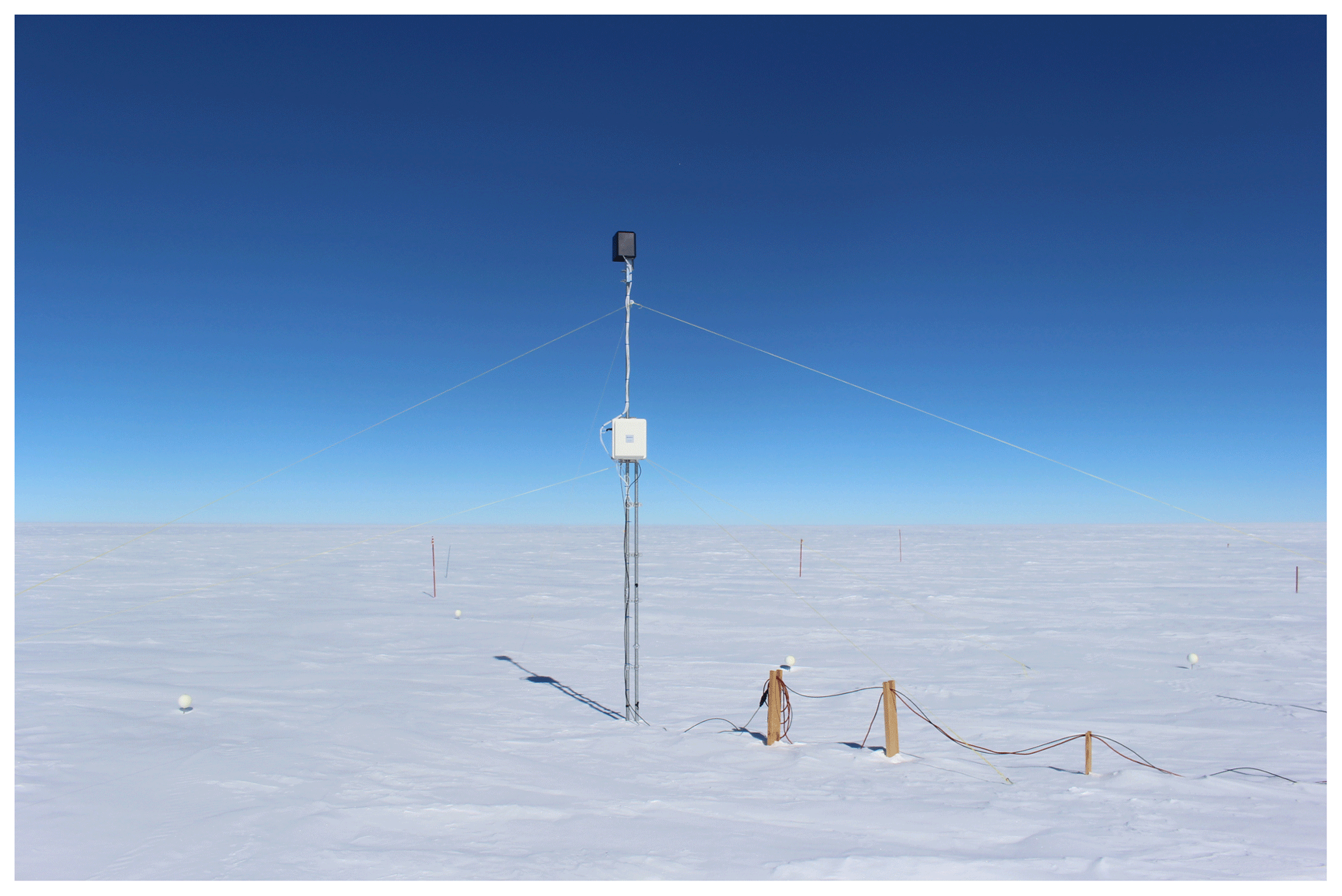
Figure 1The RLS setup at Dome C (January 2017). The lasermeter and rotation mount are located under the black cap. The control is in the white box. The photograph looks southward, facing prevailing winds, and the scanned area is behind the RLS mast.

Download

2.2 RLS precision and stability

To capture the small accumulation that occurs at Dome C, the accuracy and precision of the instrument are critical. In Picard et al. (2016) we estimated the vertical long-term absolute accuracy to be better than 1 cm over period 1. This is reasonably low compared to the annual accumulation (approximately 8 cm). To achieve such long-term stability, the mast was anchored to a wooden board (50 cm×50 cm) buried at a depth of 1 m. The mast was secured with three Dyneema SK78 ropes (3 mm in diameter) during period 1 and with six ropes on two levels during period 2 (as shown in Fig. 1). These ropes have a small wind surface area, low stretchability due to creep and weak thermal dilatation. We also estimated over period 1 that the precision (or reproducibility) between successive measurements was better than 0.5 cm.

Since the RLS was set up higher during period 2, we briefly reevaluate the accuracy here. Figure 2 shows the vertical movements of the calibration spheres (visible in the photograph in Fig. 1; see details in Picard et al., 2016). Four spheres were installed at the beginning of period 1 in the scanned area, and during period 2 only two of them remained in the scanned area, high enough above the surface to be detected, and one was added. The results show apparent movements of up to 2–4 cm in maximum amplitude over the 2 years and 0.28–0.68 cm rms over period 1 – depending on the sphere, so 0.5 cm on average for the available spheres – and 0.49–0.81 cm rms over period 2. We can estimate that the slow variations and some of the sharp variations are caused by the imperfect stability of the mast and, as noticed by the winter-over staff, by the formation and removal of hoar on the spheres (about 1 cm thick) (Champollion et al., 2013). Conversely, most of the rapid variations are likely caused by instrumental errors and the uncertainty in the detection of the spheres. The rapid variations can be quantified by computing the standard deviation of the sphere elevation changes between every successive scan. We find variations of 0.16–0.24 cm rms and 0.38–0.62 cm rms for the two periods. The largest value is obtained for sphere 5, which is at the furthest edge of the scanned area, and thus represents the most challenging conditions to retrieve the elevation. These values provide the upper limits of the instrument error.

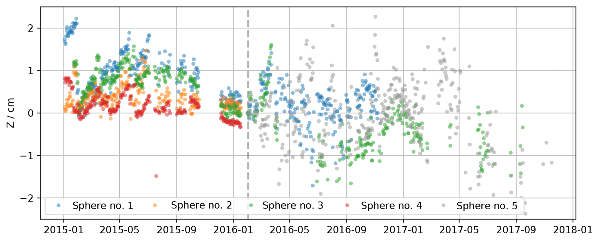
Figure 2Evolution of the elevation of five calibration spheres set up in the scanned area at the beginning of period 1. The gray dashed line shows the beginning of period 2.

Download

Another approach to estimate the non-systematic instrument error can be based on the measured rms change between successive acquisitions, which is the sum of the real rms changes and the rms variations due to the instrument error. We can thus estimate the latter when the surface has been subject to no real change, i.e., when the first term is null. Because both terms are strictly positive, we can estimate the rms variations caused by instrumental errors by searching for the minimum rms changes over the time series (i.e., standard deviation of daily accumulation) and assume that for that day, the surface did not change. For periods 1 and 2, respectively, we find minimum rms variations of 0.03 and 0.13 cm, which are very low values. These estimates are representative of the most favorable conditions (calm air), as it is likely that windy conditions always provoke real changes, and thus cannot lead to a minimum rms. We therefore conclude that the actual instrument error that most affects our daily accumulation is between the estimate derived from the spheres and the estimate derived using the minimum variations in rms, say around 0.2 and 0.4 cm for periods 1 and 2, respectively.

2.3 RLS data processing

Processing the raw data to produce elevation maps on a common and regular grid is performed in several steps. For each single acquisition, raw data comprise the radial distance and two angles (azimuth and zenith). After filtering the obviously erroneous distances (less than 3 m or more than 17 m), the data are projected into Cartesian coordinates (x,y) with z the vertical axis. z(x,y) is the surface elevation. A second filter is applied to remove the points (x,y) with fewer than two neighbors in a 5 cm radius circle centered at (x,y) and with $\left|z\right(x,y)-\overline{z}|>\mathrm{5}\mathrm{cm}$, where $\overline{z}$ is the averaged elevation of the neighbors. This operation removes outliers and small objects like blowing crystals or the RLS mast guylines. This set of curated but irregularly spaced points is then interpolated onto a regular grid using the bilinear method interpolation provided by the matplotlib.mlab.griddata Python function (version 2.2). The grid spacing is set to 2 and 3 cm, respectively, for periods 1 and 2, in relationship with the different setup heights. To avoid filling large gaps with the bilinear interpolation, a grid point was attributed a valid z value only if at least one measurement was taken within twice the grid spacing (i.e., 4 and 6 cm for periods 1 and 2 respectively) around it. In practice, we found that 93 % (62 %) of the grid points have at least one measurement within one (half) grid spacing. If the final map contained fewer than 100 000 valid grid points, it was completely discarded. All these operations yield a time series of elevation maps on a common grid. The grid orientation was determined by observing the shadow of the RLS mast in the scanned area. We found that the x axis lies towards 116^∘ (east-southeast), which allowed us to draw the southern direction on the maps. Note that this orientation was chosen to minimize the perturbation of the mast on the surface, the prevailing winds being from the southeast–southwest sector.

Various additional datasets are then derived from the generated maps. The accumulation between every successive scan is calculated as the difference between the elevation for each point of the grid. In most cases, both scans are acquired 1 d apart (90 % over period 2a) so the computed accumulation is representative of the daily variation. However, due to scan failure or rejection during the processing, longer time intervals are present in the time series (2 d in 7 % of the cases, and 3–9 d in the remaining 3 %). We nevertheless interpret the accumulation time series as if it were daily accumulation only.

The age of the snow on the surface is another dataset derived from the elevation maps. The algorithm is applied independently for each point as follows. For each point, the age is initialized to 0. For each date i the accumulation a_i since the last detected deposition or erosion event (or the beginning of the time series) is calculated. If a_i is larger than a given positive threshold δ_a, (a_i≥δ_a), there was deposition of new snow, and the age is reset to 0. If this value is lower than a negative threshold δ_e (a_i<δ_e), snow was removed by erosion, and for values between both thresholds (${\mathit{\delta }}_{\mathrm{e}}\le a_i<{\mathit{\delta }}_{\mathrm{a}}$), the variation is considered insignificant and the age is incremented by the time elapsed since the previous available date. In the case of erosion, the algorithm then searches back in time for the first date j for which the elevation was equal (or closest below) to the present elevation at the point. The snow present at the surface at date j now emerges again. The age of this snow is calculated as its age at date j plus the time elapsed since j, that is i−j. We choose a threshold value δ_a=1 cm which tends to avoid sporadic age change for small variations (possibly due to residual noise) and δ_e=0. This algorithm is robust because even if δ_a is chosen too close to the noise level, age errors are not accumulated over time, and only the statistics of the age at a given date may be affected. A low threshold tends to bias the age distribution towards younger snow due to the overestimation of new snow accumulation. To illustrate the sensitivity we also present results for δ_a=0.5 cm and ${\mathit{\delta }}_{\mathrm{e}}=-\mathrm{0.5}\mathrm{cm}$.

In addition to the age, we derive the time of residence on the surface, which is the same as the age except that when erosion is detected, the time on the surface at time i is taken as equal to the time on the surface at time j, not counting the time spent while buried (i−j). We also derive the time of residence before erosion, which is equal to the time spent on the surface just before erosion is detected.

2.4 Meteorological data

Meteorological data are used to relate surface changes and weather. We use precipitation forecast provided by the ERA-Interim reanalysis (ERA-I) (Dee et al., 2011) near Dome C. Due to the absence of reliable methods to record in situ precipitation in Antarctic conditions, ERA-I is one of the most reliable sources of information to date (Bromwich et al., 2011), though it is known to underestimate accumulation near Dome C (Genthon et al., 2015; Wang et al., 2016). For wind speed and direction, we use data from the weather station at Concordia station (75.1^∘ S, 123.3^∘ E, 3230 m a.s.l., http://www.climantartide.it/, last access: 15 July 2019). Over the 3 years, the mean wind speed at 3 m is 7 m s⁻¹, which is higher than the ERA-I prediction of 5.2 m s⁻¹ at 10 m. Nevertheless, both sources agree on the temporal variations, with a correlation of 0.8, which is the most important point for our comparison. The wind regime at Dome C is characterized by a prevailing direction from the south (74 % of the time), the most likely direction being 190^∘. The distribution and maximum remain identical when selecting only strong winds (e.g., over the mean, 7 m s⁻¹), which are relevant for this study.

3.1 Surface elevation changes

The elevation of the surface averaged over the scanned area generally increases with time at a mean rate of 8.7 cmyr⁻¹ (Fig. 3). However, different dynamics are observed for the different years. As noted by Picard et al. (2016) for the first year, a unique and marked accumulation event occurred in the period 4–16 July 2015, which accounted for most of the annual accumulation during that year. In contrast, the second and third years of the dataset feature a fairly regular increase in the surface elevation, suggesting the absence of dramatic accumulation events. Interestingly, this regularity in the cumulative precipitation is also found in the ERA-I forecast (Fig. 3, green curve) with a remarkable absence of seasonal signal despite the huge variations in temperature between summer (typ. −25 ^∘C) and winter (typ. −70 ^∘C). However, the precipitation in ERA-I is overall too weak with only 16 $\mathrm{kg}{\mathrm{m}}^{-\mathrm{2}}{\mathrm{yr}}^{-\mathrm{1}}$ over the 3 years. This mass is equivalent to only 5 cm yr⁻¹ of snow taking a typical surface density value of 320 kg m⁻³ for the conversion (Genthon et al., 2015; Picard et al., 2014; Leduc-Leballeur et al., 2017). The missing mass in ERA-I could be due to underestimation of the synoptic precipitation or of the deposition that seems indeed very low (Genthon et al., 2015) compared to that reported by other sources (Krinner et al., 2006; Agosta et al., 2019).

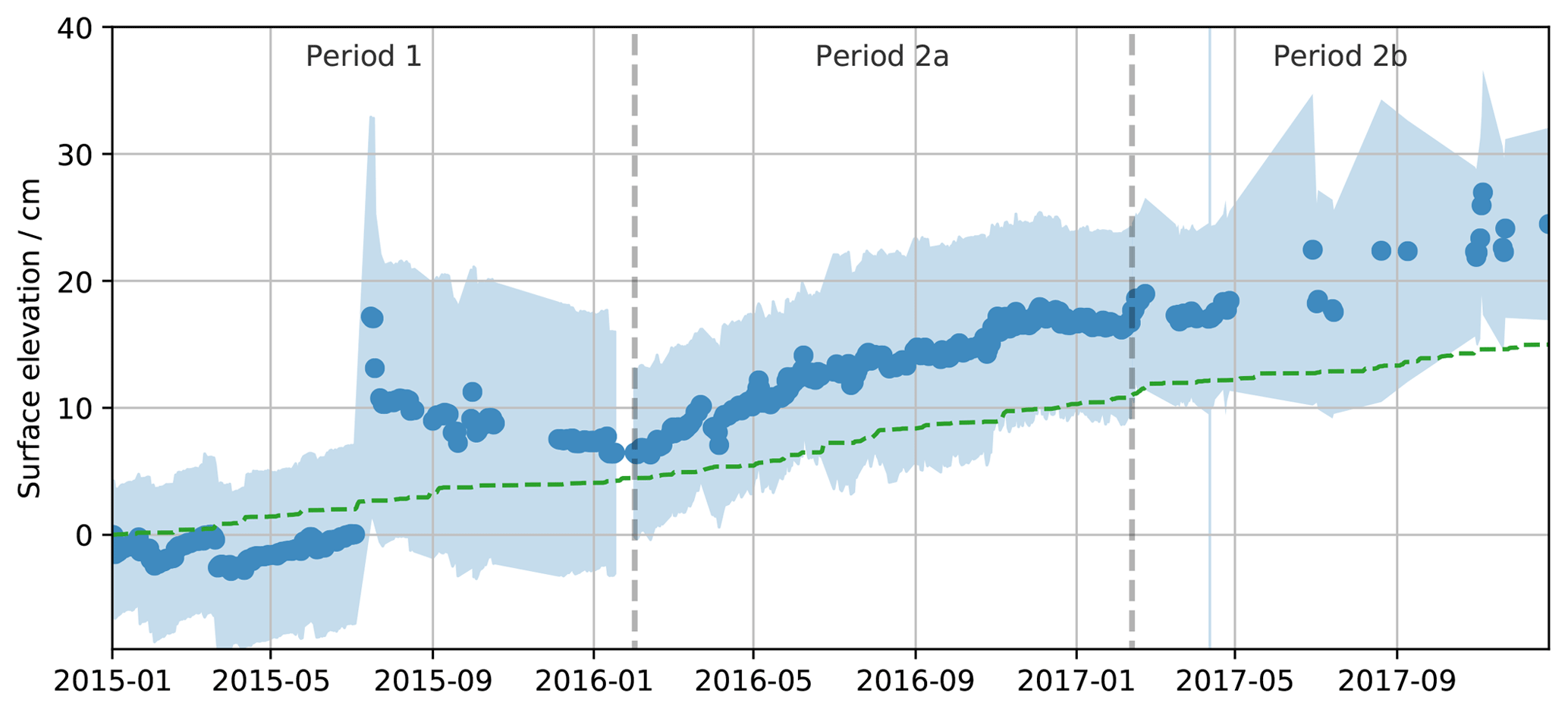
Figure 3Evolution of the mean surface elevation and rms height in the scanned area observed by RLS (blue) and of the cumulative precipitation forecast from ERA-Interim at Dome C (green) converted in snow depth assuming a surface density of 320 kg m⁻³. The blue shade shows ±1 rms height around the mean.

Download

The root-mean-square height of the surface (rms height, calculated as the standard deviation of the surface elevation) is shown in Fig. 3 as a blue shaded area. Physically, this metric measures the amplitude of the elevation variations over the scanned area including all the spatial scales of variations, that is, those due to the meter-scale roughnesses, the local slope, and potential instrumental artifacts (such as the repeatability error of the RLS). Overall, the rms height has a large magnitude compared to the annual accumulation. Over the 3 years, it was smaller (4 cm) at the beginning of the first season, before the event in July 2015, where it nearly doubled and remained fairly constant after that, with 7–8 cm. In particular it remained constant during the shift periods 1 and 2a, despite a 3-fold increase in the scanned area. These numbers are significant compared to the instrumental error (Sect. 2.2), except during the last period (2b), where we believe the standard deviation is unreliable, and probably affected by the failures of the RLS.

To estimate the respective role of the meter-scale roughness and the local slope over the scanned area, we fitted a plane on each scan using the least-square method. The local slope is fairly constant, of the order of 1–1.5^∘ over the time series, indicating that a large-scale terrain undulation was present. In comparison, the Dome C area has a very small overall slope, less than 1 m per kilometer (0.06^∘). Once the plane is subtracted from the elevation map, the rms height is reduced by about half, implying that half of the elevation variations are attributed to meter-scale roughness (typically sastrugi and small dunes) whilst the other half are caused by terrain undulation (e.g., decameter-scale dunes; Picard et al., 2014). It is finally worth noting the absence of seasonal signals in the roughness evolution, which differs from reports for other locations on the ice sheet (Gow, 1969; Adodo et al., 2018).

3.2 Spatial characteristics of the annual accumulation

Figure 4 shows the statistical distribution of annual accumulation over the scanned area. The three periods, corresponding roughly to the years 2015, 2016, and 2017, present different patterns. In 2015, the mean accumulation is 7.7 cm and the highest accumulation is nearly 30 cm. Negative accumulation concerns 12 % of the surface. The second year highlights a significantly higher mean accumulation with 10.0 cm (+31 % compared to 2015), which is also present in ERA-I (+50 % precipitation). It results that almost no negative accumulation is observed, but more surprisingly the maximum accumulation is reduced compared to 2015, from 30 to about 22 cm. The accumulation distribution in 2016 looks Gaussian and narrow in contrast to the two other years showing a wider and more asymmetrical distribution. The last year has the same mean accumulation as the first one, but fewer negative accumulation values and a lower maximum accumulation, of the order of 22 cm.

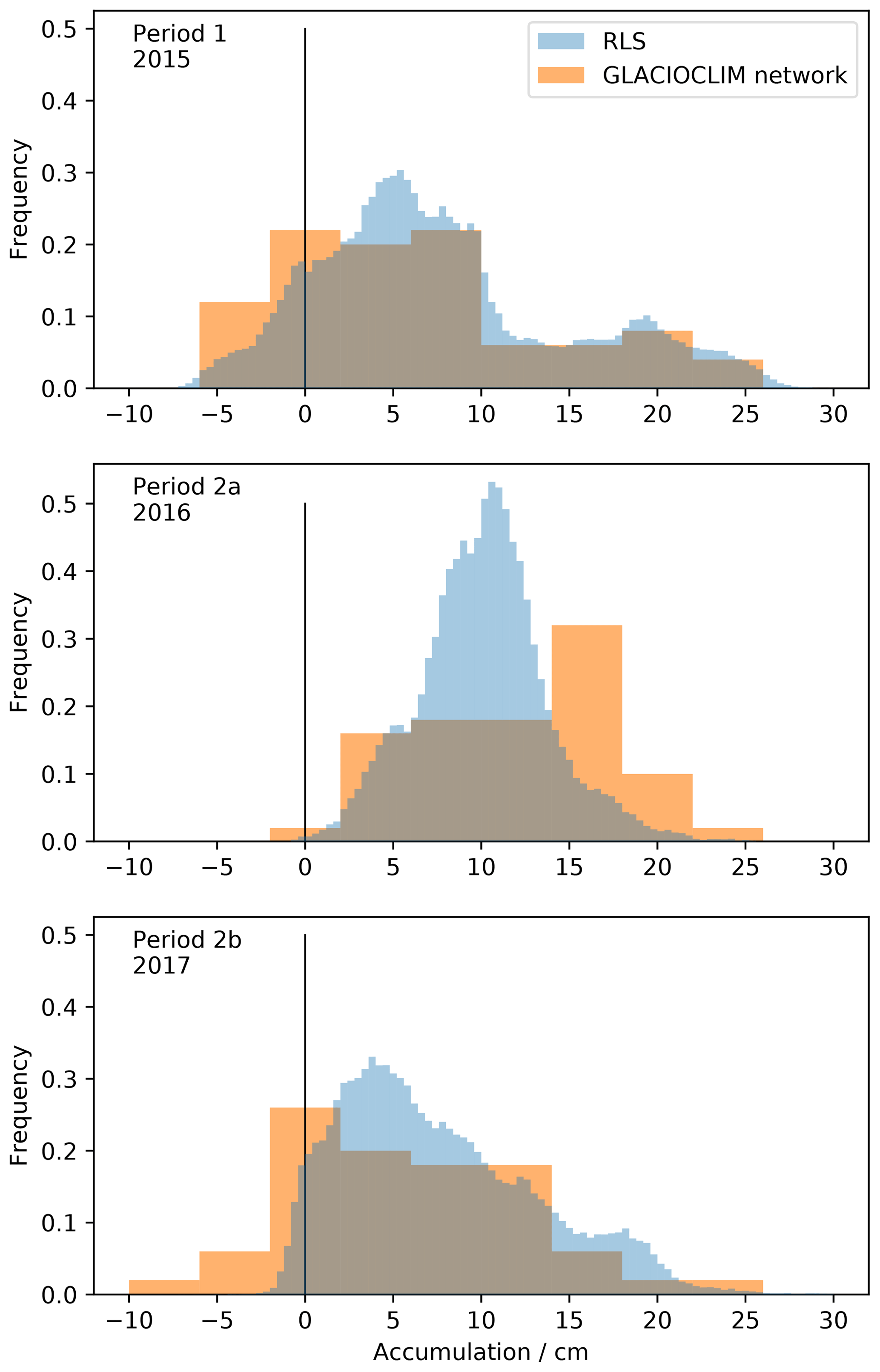
Figure 4Distribution of the annual accumulation in the scanned area (blue bars) and from the 50 stakes of the GLACIOCLIM network near Dome C (orange bars).

Download

In Picard et al. (2016), the distribution of annual accumulation estimated over the RLS area of 40 m² in 2015 was noticed to be surprisingly similar to the distribution obtained from the GLACIOCLIM stake network, which is composed of 50 measurement points about 10 m apart, thus covering a much more extensive area. Figure 4 further confirms this finding for the two last years (2016 and 2017). This remarkable result indicates that despite the small extent of the RLS scanned area, the distribution of net annual accumulation may be representative of a wider area.

3.3 Spatial and temporal characteristics of the daily accumulation

The mean and standard deviation of accumulation (noted $\overline{A}$ and σ_A, respectively) between every two consecutive dates (called daily accumulation here despite the irregular sampling in time) were calculated and compared to precipitation (from ERA-I), wind speed, and direction (from the Concordia Automatic Weather Station). Figure 5 shows scatter plots between these variables (except wind direction as no interesting signal was found). Overall, there is little correlation, if any, between the variables, which is unexpected because in many regions of the world the daily accumulation is strongly related to precipitation (e.g., Alpine regions), and in Antarctica the role of the wind has been emphasized (Groot Zwaaftink et al., 2013). This role may be the reason why in the bottom left plot in Fig. 5, points are scarce above the orange line delineating a domain with low-wind and high surface change. This indicates that some wind is necessary to induce surface change, which is obvious, though the statistical relationship is probably not robust. Another interesting and more robust pattern is visible in the bottom right plot showing the mean and standard deviation of the accumulation. This pattern indicates that significant (positive or negative) mean accumulations are always associated with high standard deviations over the area, which can be expressed mathematically by ${\mathit{\sigma }}_A>\left|\overline{A}\right|$. We interpret this relationship by the fact that (1) many events change the surface but do not affect the overall mass in the area (${\mathit{\sigma }}_A\gg \left|\overline{A}\right|\approx \mathrm{0}\mathrm{cm}$) and (2) that the events leading to significant accumulation or erosion cause highly heterogeneous changes over the area (with both negative and positive changes). Conversely, the process of accumulation or erosion by “layer” (which would correspond to ${\mathit{\sigma }}_A\ll \left|\overline{A}\right|$) does not exist at Dome C. However this relationship does not link accumulation to meteorological conditions.

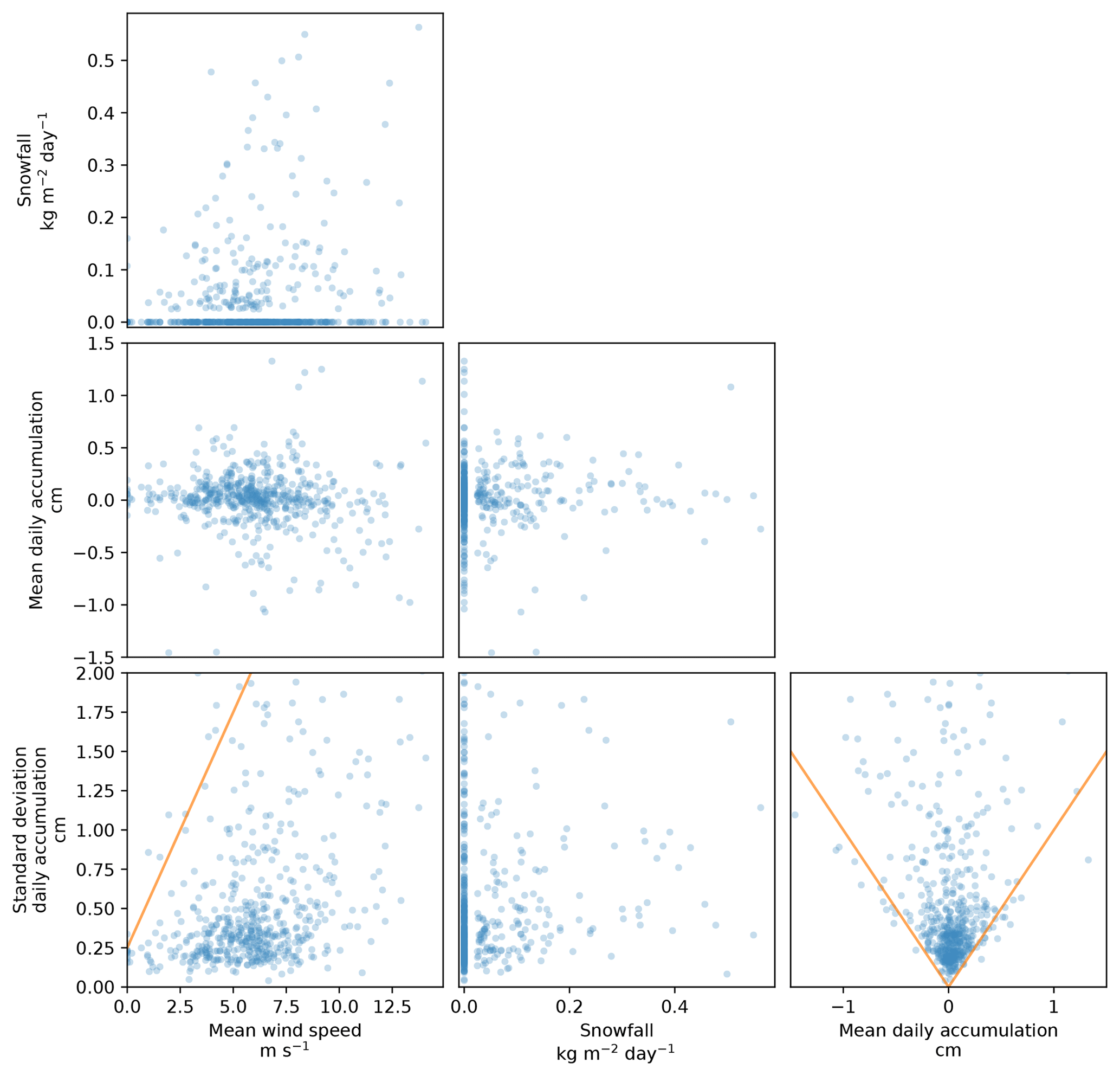
Figure 5Comparison between mean daily accumulation, standard deviation of daily accumulation, daily snowfall, and mean daily wind speed including data from the 3 years. The orange lines delineate remarkable zones with few data (see Sect. 3.3).

Download

This result suggests that further investigation concerning the positive and negative changes in surface elevation at every point is necessary. Figure 6 shows the cumulated sum (average over the scanned area) of daily accumulation considering either only the increments (deposition above 0, 0.5, or 2 cm) or the decrements (erosion higher than 0, 0.5, and 2 cm). To account for the instrumental error in the data, we have estimated for each increment a (or decrement) the probability of the presence of an error by assuming that the error follows a normal distribution with a standard deviation of 0.4 cm (Sect. 2.2), and with the probability set to 1 for 0 cm increments, that is $p\left(a\right)=\exp \left(\frac{-a^{\mathrm{2}}}{\mathrm{2}{\mathit{\sigma }}_{\mathrm{a}}^{\mathrm{2}}}\right)$. We then randomly removed every increment a in the proportion of the probability p(a), that is, given $x\sim \mathcal{U}(\mathrm{0},\mathrm{1})$, the increment a is rejected if x<p(a). The figure also shows the net cumulative accumulation for comparison, which is exactly the same as the mean surface elevation changes in Fig. 3. Over the 1-year period, each pixel has received a total of 55 cm of snow on average. Most of it has been removed (47 cm, or 85 %), leaving a final net accumulation of about 10 cm (Sect. 3.1). The ratio between deposition and net accumulation suggests that a snow particle is remobilized at least $\mathrm{55}/\mathrm{10}=\mathrm{5.5}$ times before its definitive settling. This value is to be taken with caution because of the limited frequency of the scans that only allow us to probe the “long-term” deposition–removal cycles, which excludes the rapid rebounds that occur during saltation and blowing snow. We additionally computed the increments above 0.5 cm (this value is twice as large as the RLS precision). These “significant” events of deposition bring 50 cm of snow in a year, which is still much larger than the net annual accumulation and again suggests that snow is subject to many deposition–removal cycles. Interestingly, the increments above 2 cm (call hereinafter “major events” as they each represent more than a fifth of the annual net accumulation) amount to 22 cm, meaning that every pixel receives many times a year at least 2 cm of snow in a single day (or a few days for the few cases the scanner was not working). The process of erosion shows similar behavior, with 18.3 cm removed by events larger than 2 cm on average over the area.

Figure 6Cumulative spatially averaged amount of snow accumulated (blue >0) and eroded (green <0) in every pixel during the period February 2016–February 2017 (period 2a). Only events with accumulation over the threshold 0.5 and 2 cm and erosion below the thresholds −0.5 and −2 cm are taken into account for the lighter blue and green curves. Cumulative net accumulation is shown in black.

Download

Overall, the results of this section depict a surface subject to frequent changes that remain invisible to the observers who only access long time-period averages or spatial averages of accumulation. To further explore the accumulation process, in the next section we focus on the major events, which amount to 22 cm.

3.4 Patchy accumulation

Figure 7 shows the accumulation map between 4 and 16 July 2015 corresponding to the exceptional event raising the surface by 17 cm on average and clearly visible in Fig. 3. We are confident that this is not an artifact because the surface elevation remained affected by this event for months, and the calibration spheres confirm the stability of the setup. Unfortunately, no data are available between 4 and 16 July, preventing a precise description of the sequence of this event. This RLS failure was likely caused by snow jamming the lasermeter window, which leads us to suppose that intense snow drift started at the beginning of this period, right after 4 July 2015. This event is the only one raising the surface as a whole and smoothly. Nonetheless, the accumulation is not even, featuring a trend, with x increasing from nearly 0 cm (left corner in the figure) to 40 cm over a distance of about 10 m (right corner). This corresponds to the decameter-scale dune mentioned above.

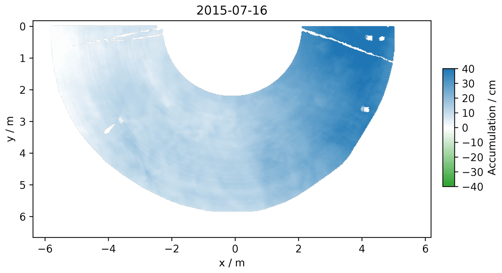
Figure 7Accumulation between 4 and 16 July 2015.

In contrast to this rare event, accumulation maps usually look different. This is illustrated by the maps of accumulation between 28 and 29 May 2016 and between 29 and 30 May 2016 (Fig. 8). It is worth noting that the x- and y-axis scales and the color scale are different from those in Fig. 7. The first day, the net accumulation is −0.8 cm, with 80 % of the area in erosion (and 75 % in pronounced erosion (>2 cm)). The second day, the accumulation is +0.3 cm with 62 % of the area in accumulation. In both cases, elongated patterns are clearly visible. The second day it is possible to observe that most erosion patterns correspond to the accumulation patterns of the previous day (e.g., the two large blue areas on the left the first day are green the second day), meaning that most of the accumulation features in the first day have been blown away and replaced by new ones with similar shapes (size, elongation, orientation).

To explore the geometrical characteristics of these deposition patterns, that we called patches, we applied a threshold (2 cm) to the daily accumulation maps and segmented the map. Each individual patch then received a unique label and its geometrical properties were computed using the Python function skimage.measure.regionprops. The properties include area A, eccentricity e and major axis length of the best-fitting ellipse (0 indicates a circle and 1 an infinitely thin segment), and the orientation of the major axis (with respect to north, increasing eastward). Figure 9 reports the orientation and eccentricity of the elongated patterns only (e>0.8). On 29 May 2016, it is clear that the patches were aligned with orientations ranging from 140 to 192^∘ with respect to the north. The average orientation is 174^∘ (we applied weighting proportional to Ae² to account for the size and eccentricity). This orientation is nearly south, which unsurprisingly corresponds to mean wind direction of the day (169^∘) and to the prevailing wind direction (Champollion et al., 2013). The same computation is repeated for the 280 d of period 2a, yielding 1103 patches that appeared for 93 different days (33 % of the time). As found before for the mean accumulation, there is no clear relationship between the patch properties and wind speed (not shown). The most marked relationship is between the daily-mean orientation and the wind direction on the same day (Fig. 10) with a correlation of 0.33 (the correlation is weighted by the number of patches as in Fig. 10). This simply means that the patches form longitudinal dunes or sastrugi approximatively aligned with the wind direction.

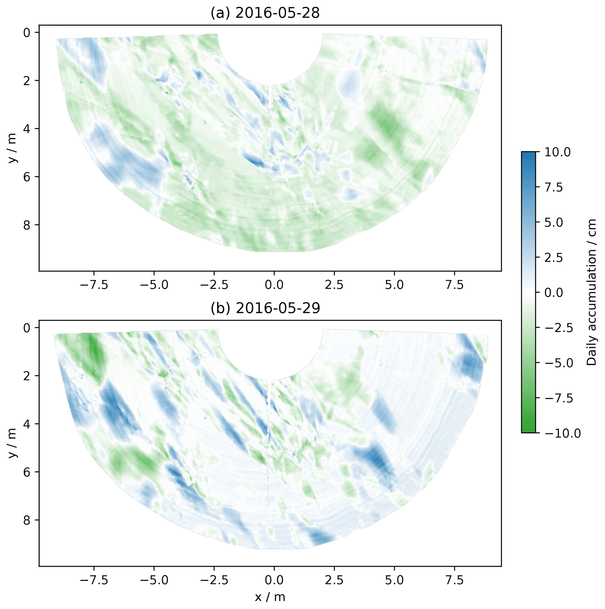
Figure 8Accumulation between 28 and 29 May 2016 (a) and 29 and 30 May 2016 (b).

As a consequence of the frequent deposition–removal cycles, many patches studied here are ephemeral. They can be rapidly removed by the next wind event following their formation, as highlighted on the sequence of 29 and 30 May 2016. These ephemeral patches do not contribute to the snowpack in the long term. To capture and investigate more specifically the few patches that remain and settle and that in the end are the important ones for the snow mass balance and the snowpack internal structure, we estimated the time of survival as follows: for each patch detected at time i, we compute its initial volume (between the surface at time i and the surface at time i−1) and how this volume evolves at all times $i^{\prime }>i$ (volume between the surface at time i^′ and the surface at time i−1). More precisely we seek the minimum value of this volume and the date at which this minimum is reached. The patch is fully eroded if the minimum volume is 0 cm³ or negative, which happens for 652 of the patches among 1103 detected in period 2a (59 % of the cases). Partial erosion occurs when the minimal volume is between 0 and the initial volume, which concerns all the other patches. We found none being fully and continuously buried after deposition in our dataset. Full or partial erosion of at least half of a patch volume occurs for a large proportion of them (930, i.e., 84 %). The mean time of survival before full erosion is 17 d, and for partial erosion this time increases to 46 d, meaning that partial erosion is typically possible after a longer period. In other terms, if a patch is not removed soon after deposition, it is increasingly harder to remove it. The calculation of the time of residence before erosion (Sect. 2.3) provides similar information while not being limited to patches (accumulation over 2 cm). The time of residence on the surface before erosion is 15 d on average over period 2a, with a large spread (10 d standard variation). The maximum is 129 d.

This result confirms that deposition–removal of snow is a very common process and that only a small part of the deposited snow remains on the surface and contributes to the snowpack. Moreover, even when the snow is removed, the number of days spent on the surface can be significant, which lets metamorphism operate and modifies the physical and chemical properties of the snow before it is removed and blown away.

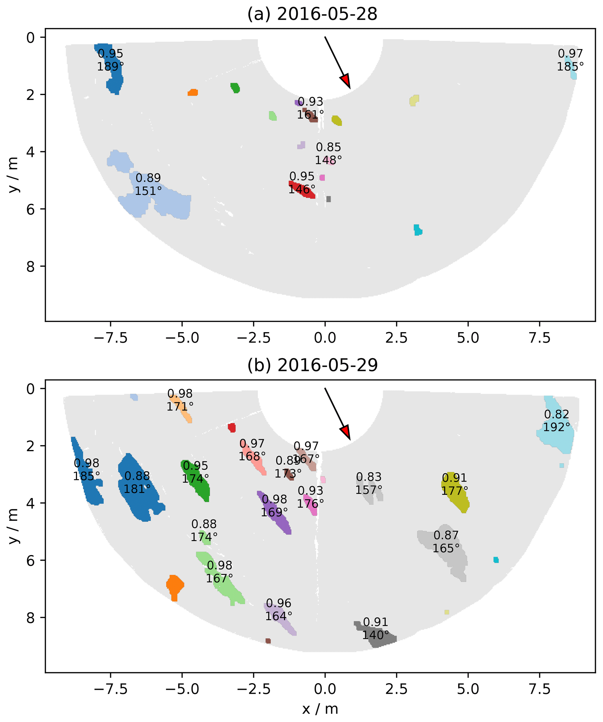
Figure 9Patches of accumulation (>2 cm) between 28 and 29 May 2016 (a) and 29 and 30 May 2016 (b). For each patch with sufficient elongation, the circularity and the orientation are indicated. The southern direction (180^∘) is indicated by the red arrow.

Figure 10Daily-mean orientation of the accumulation patches as a function of the daily-mean wind speed. The size of the symbols indicates the number of patches.

Download

3.5 Age of the snow on the surface

We estimate the age of the snow on the surface with the algorithm described in Sect. 2.3 for all the scans. Figures 11 and 12 show the age of snow near the end of period 2a (18 and 27 January 2017) with respect to the beginning. We have chosen these dates because they are less affected by the fault that increasingly affected RLS from February 2017. To highlight the sensitivity of the algorithmic choices, the histogram in Fig. 12 shows as white dotted bars the result of processing the scans with symmetrical thresholds for accumulation and erosion.

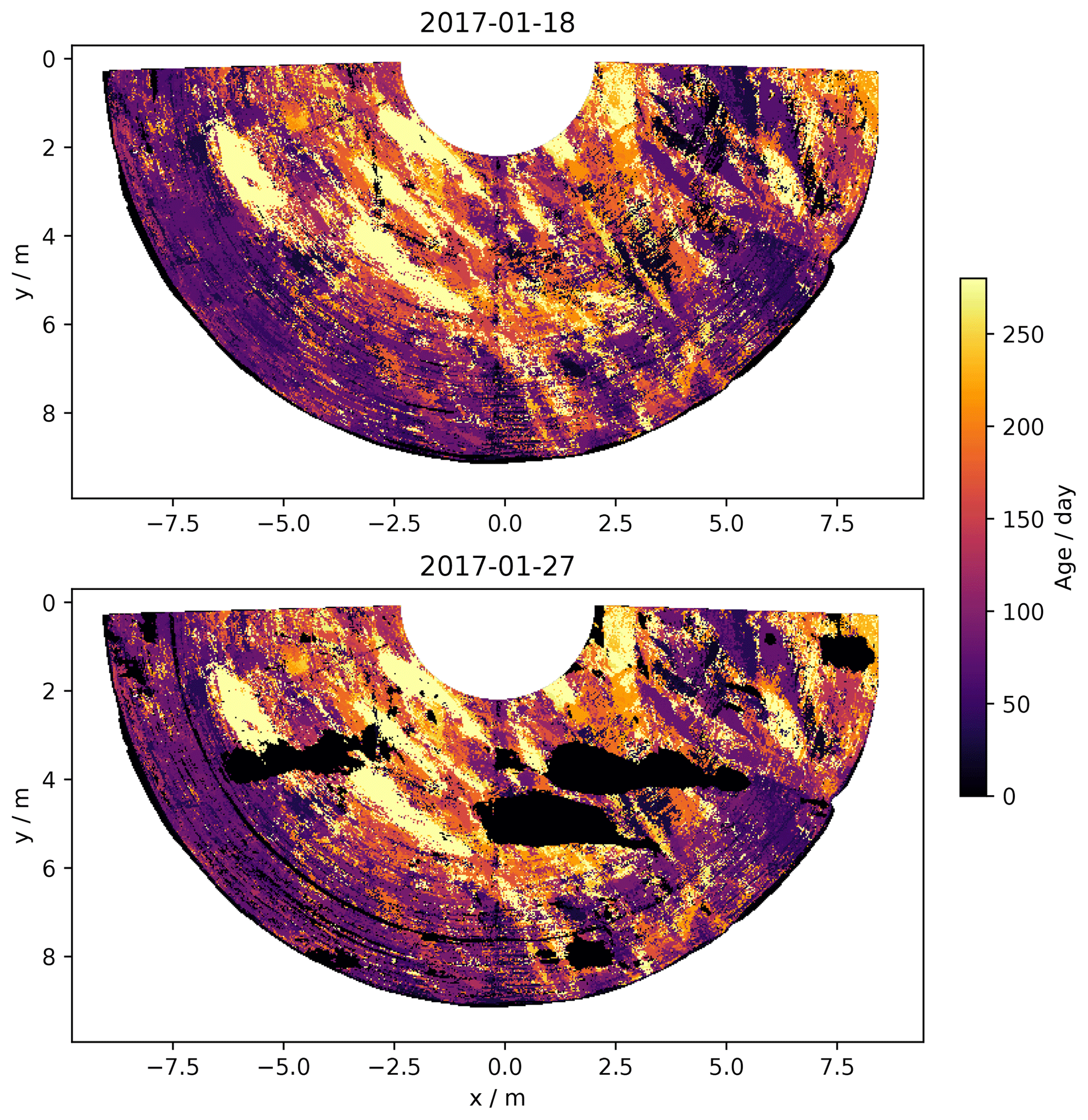
Figure 11Map of age of the snow on the surface for two dates.

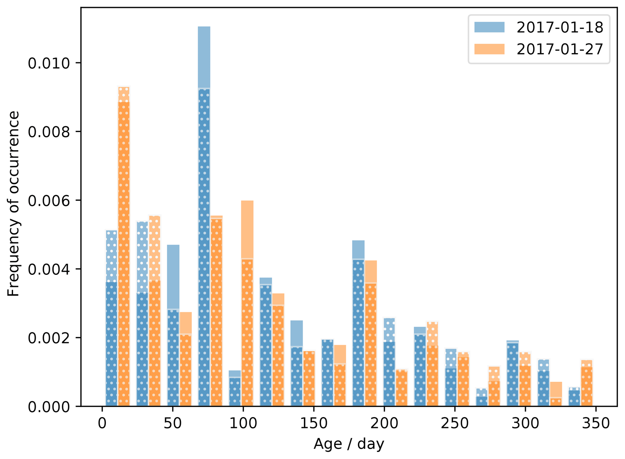
Figure 12Distribution of the age of the snow on the surface for two dates (blue and orange). The age is determined using the algorithm described in Sect. 2.3 based on the accumulation and erosion thresholds δ_a=1 cm and δ_e=0 cm (solid colored bars) and δ_a=0.5 cm and ${\mathit{\delta }}_{\mathrm{e}}=-\mathrm{0.5}\mathrm{cm}$ (white dotted bars).

Download

The map and the distribution of age show that snow with very different ages is present on the surface, from 0 (accumulation of the day) to the maximum possible given the duration of the time series. About 48 % of the surface is younger than 100 d (which is thus the approximate median age), while about 24 % is older than 200 d and 10 % older than 300 d. These figures are moderately affected when using the algorithm with the symmetrical thresholds (46 %, 30 %, and 14 %, respectively).

These proportions also change from day to day because of the ephemeral deposition–erosion as illustrated on 27 January 2017 (Fig. 11) where a few patches of recent accumulation covered 11 % of the surface. These patches disappeared the day after (data not shown), forming the surface as shown in the 18 January map. It is also clear from the histograms that almost all ages are present at the same time, which is in agreement with the apparent regularity of the accumulation (Fig. 4).

Note that period 2a had a relatively high net accumulation and narrow spatial distribution of accumulation, so it is likely that the distribution of age shown here could be wider for years with less accumulation.

The age maps provide another interesting piece of information. We can indeed see clear patterns with marked alignments on these maps (Fig. 11). This confirms the patchy nature of the accumulation process already noted in the previous section (Sect. 3.4). We indeed showed that a significant part of the daily accumulation over 2 cm is organized in patches but that most of them (59 %) do not contribute at all in the long term to the surface mass balance. Here, we complement this by showing that some of the partially eroded patches remain clearly visible on the surface even after a year.

3.6 Structure of the snowpack

The accumulation process depicted in the previous section may affect the internal structure of the snowpack and its spatial variability. The burial of the snow can be tracked using the RLS, at least over a short depth given the limited length of the time series. Figure 13 shows the snowpack internal structure along the x-axis transect at y=4 m (see, e.g., Fig. 11) at the end of period 2a. It is obtained, assuming no compaction, by plotting the successive positive increments of surface elevation at each point with a color depending on the date of deposition. The gray color marks snow older than the first day of period 2a (1 February 2016). The z origin corresponds to the mean elevation in the whole scanned area at the beginning of period 1. The two gray lines represent the mean at the beginning and end of period 2a, respectively.

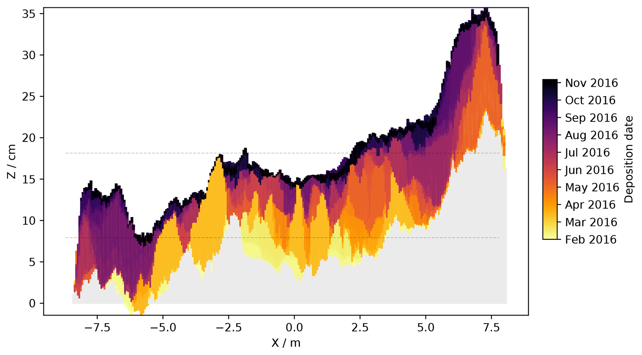
Figure 13Snowpack internal structure along the transect parallel to the x axis at Y=4 m deduced over the period February 2016–February 2017 (period 2a). The color indicates the date of deposition of the layer. The gray shade corresponds to snow older than the first acquisition of RLS in this period. The two gray lines represent the scanned-area average surface elevation at the beginning and end of period 2a.

It is remarkable that the figure shows distinct coherent patterns and fairly little noise. The figure confirms that the heterogeneity on the surface transfers into the snowpack. For instance, around x=0 m old snow is present at 11 cm under the surface (yellow) whilst the surface is young (black). This area presents the greatest diversity in terms of age and the largest number of distinct layers. Around $x=-\mathrm{3}\mathrm{m}$ in contrast, the whole accessible depth features a single homogeneous layer formed in March 2016 (orange). Another thick homogeneous layer is found around $x=-\mathrm{7.5}\mathrm{m}$ but it is much younger (violet, August 2016). Even where we do not observe a unique layer, it is clear that only a few events (≈5) have contributed to the snowpack, forming a few distinct layers. Conversely, it means that at every point many deposition events occurring during a year are not represented, which implies that the profiles of snow physical and chemical properties are probably very different from one point to another.

Another remarkable feature is around x=7.5 m where we can see a 10 cm high dune deposited in July 2016 (orange) where the surface was already higher than the surroundings as marked by the gray lines. Then, two successive events (in September and November, violet) accumulated more snow on the sides of this dune, which was then about 15 cm higher than the surrounding surface. This may be the result of interaction with the pre-existing dune leading to preferential deposition on one side, here the windward side. A similar behavior is observed around $x=-\mathrm{4}\mathrm{m}$ where the space between the two small dunes (in light orange) has been filled by some subsequent events.

4.1 Temporal perspective

The RLS provides contrasted results regarding the surface evolution depending on the spatial scale of interest. On the one hand, the time series of surface elevation averaged over the whole scanned area depicts a slow and relatively regular accumulation, without seasonality or rapid events, except a single event which raised the surface by 8 cm in a few days during the first winter of observation. The accumulation rate measured by RLS ranges between 8 and 10 cm yr⁻¹ for the 3 years of observation, which agrees with values reported by previous studies for Dome C (e.g., Petit et al., 1982; Urbini et al., 2008). The time series of rms height (standard deviation of the surface elevation) is also relatively steady, which again suggests that only slow changes occur over the scanned area. This overall stability is further illustrated in the sequence of photographs in Fig. 14. The photographs were taken from 20 m above ground at Dome C. They depict a landscape dominated by barchan dunes with few differences between the pictures of January and December 2017, 11 months apart. This steadiness is surprising because the accumulation over this period has been of the order of 8 cm, the typical annual accumulation expected in the area (Petit et al., 1982; Genthon et al., 2015).

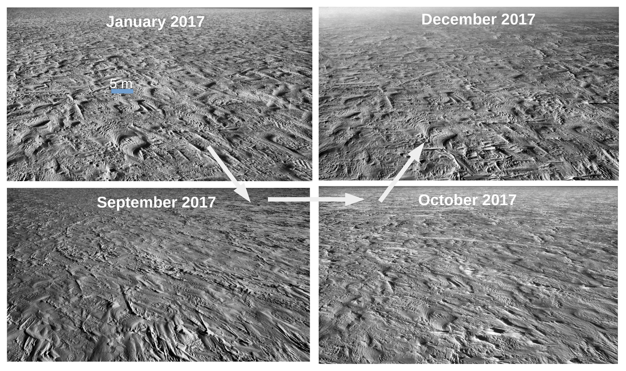
Figure 14Photographs in the near infrared range (820 nm) taken from 20 m height at Dome C (75^∘ S, 123^∘ E) in Antarctica on 27 January 2017 (21:00 UTC), 21 September 2017 (06:00 UTC), 23 October 2017 (20:00 UTC), and 4 December 2017 (17:00 UTC) and highlighting how little the surface can have changed over nearly 1 year.

Download

On the other hand, a very different picture is obtained by investigating the daily changes in surface elevation (i.e., the daily accumulation) and the small spatial scales. Indeed, many local changes in elevation affect the surface almost everyday. Most of these changes are however ephemeral (a few tens of days) so that the overall statistics of the surface are relatively constant or slowly changing. These changes are typically caused by migrating patches on their way downwind or remobilization of loose snow deposited by a recent storm. The picture of September 2017 in Fig. 14 illustrates how major these ephemeral changes in the landscape can be. Nevertheless, these temporarily accumulated snow masses have little consequence as far as the surface mass balance and the snowpack internal structure are concerned. However, they do have consequences on other aspects as they shield the snow surface for a few days, weeks, or even months from solar and infrared radiation and suppress the photochemistry activity and the exchanges of heat, water, and chemical components between the consolidated surface and the atmosphere. During the period of residence, these ephemeral snow masses are subject to transformations resulting in changes in their physical, isotopic, and chemical properties (Casado et al., 2018). When these masses are transported in a downwind region and deposited, they can be very different compared to fresh snow coming from direct local snowfall. This phenomenon of deposition–erosion–transport repeats itself several times. We provide a rough estimate of about five cycles before settling, considering only the timescales longer than a day, thus excluding the many rebounds occurring during saltation. We are however unable to estimate the distance traveled over these cycles.

The meteorological conditions triggering the surface changes raise an important question for modeling, but have not been elucidated here. Snowfalls seem to be frequent at Dome C according to the ERA-I reanalysis, which is in agreement with the slow and regular accumulation observed with RLS, but these events are not related to the observed changes in the surface. The occurrence of snowfalls in ERA-I has been compared to satellite data (Palerme et al., 2014; Lemonnier et al., 2018) in a coastal region and found to be reliable, but conversely it is well known that ERA-I misses a large part of the accumulation amount around Dome C (Genthon et al., 2015). Apart from snowfall, common sense suggests that wind speed should be a driver of change. Groot Zwaaftink et al. (2013) considered in a modeling study that snow deposition occurred after sustained wind over 3 m s⁻¹ for 100 h. Libois et al. (2014) similarly considered that wind speed over 7 m s⁻¹ is required to initiate drift, which then continues as long as this speed limit is reached at least once within 24 h. This criterion yields a drift rate of 70 events per year, which compares well with our estimates of 93 d with patch formation over a year. Nevertheless, our analysis has not revealed any robust simple relationship with the wind speed. The accuracy of the daily accumulation derived from RLS is limited by noise and some artifacts, which could be an explanation. However, a complex interaction between wind and the surface is also not to be excluded. For instance, wind with a direction perpendicular to the prevailing surface roughness exerts a stronger drag on the surface than when parallel, potentially resulting in stronger erosion. This effect was at least once shown on the removal of surface hoar at Dome C (Champollion et al., 2013). Similarly Amory et al. (2017) showed how drag decreased during a snowfall episode (though not at Dome C, but in a coastal region) and (Amory et al., 2016) how the surface roughness direction adjusted to the wind direction. Another key parameter, missing here in our analysis, is the cohesion of the snow (Sommer et al., 2017) that is able to modulate to a very large extent the snow mobility (Vionnet et al., 2012).

4.2 Spatial perspective

All our results show great variability at the meter scale on the surface (e.g., daily accumulation, age of snow on the surface) and within the snowpack (snow layers). Most of this variability results from the heterogeneous accumulation of snow and the selective erosion. We propose calling this former process “patchy” accumulation, in contrast to the even accumulation “in layers”, which is typical of the alpine regions. Representing this process in one-dimensional snow models is a challenge. Groot Zwaaftink et al. (2013) managed to represent the fact that most patches are ephemeral by summing snowfalls and delaying the effective deposition based on wind-speed-based criteria as aforementioned. Even though this results in thicker deposition per event than when all snowfalls are deposited independently, it is impossible with one-dimensional models to account for the fact that the patches often cover a very small fraction of the surface and therefore can be much thicker than if a snowfall is evenly deposited. This is fundamental to produce layer thickness of a few centimeters, as observed in the field, when most snowfalls bring less than a millimeter per day (e.g., 4 mm is the maximum of snow over the 3-year period in ERA-I). Only using a distributed or three-dimensional approach enables the representation of this feature. The attempts of Libois et al. (2014) (already mentioned) were a relative success with a good representation of the spatial distribution of annual accumulation compared to the GLACIOCLIM stake network. However, some of their hypotheses need to be reevaluated in light of our new results. For instance, they assumed that snow deposition only occurs in the lowest 20 % of the surface. This tends to smooth the surface, yet we have shown an example of accumulation near the highest dunes, which conversely tends to enhance the spatial variability. This may be the reason why they obtained an underestimation of the variability of the density and specific surface area profiles in the snowpack. Further work is needed to implement a process able to produce dunes and more generally to transfer the observational findings of the present study to concrete processing, adequate for numerical modeling.

It results from the patchy accumulation and the strong erosion that the surface is continuously rough at Dome C, as evidenced by the rms height. This is usually not the case in alpine regions where roughness increases after snowfalls (Naaim-Bouvet et al., 2016). Surface roughness can amplify itself because it plays the role of an aerodynamic obstacle that promotes heterogeneous deposition and the formation of new rough features overlying the old ones. Moreover, in the longer term, snow on the different faces of the roughness features is exposed to different radiation and wind shear conditions, likely leading to different evolutions of the microstructure (different sintering, sublimation, deposition, and metamorphism). The RLS is limited on this aspect. An avenue is to exploit the laser backscatter signal available from some lasermeters, to retrieve the specific surface area, micro-roughness (hoar), cohesion, and potentially other properties.

It is also worth mentioning that the patches studied throughout this paper are smaller in general than the accumulation pattern that appeared in 4–16 July 2015 (Fig. 7). The latter is probably more similar to the barchan dunes visible in the photographs in Fig. 14 and evoked in Picard et al. (2014) and Sommer et al. (2018). These dunes have tails elongated at ≈45^∘ with respect to the wind direction (Filhol and Sturm, 2015) while the small patches are well aligned with the wind direction (longitudinal bedform). These are clearly different objects, with different sizes (meter versus decameter) and different dynamics (daily versus yearly).

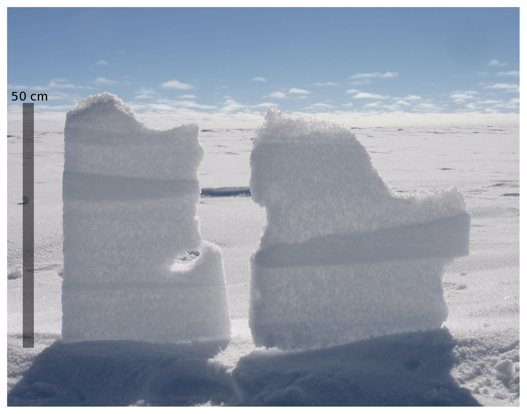
Figure 15Photograph of a thin vertical section extracted from 5 m depth at Dome C in January 2010 showing the persistence of heterogeneity at depth.

Download

4.3 Snowpack perspective

The heterogeneity of the surface eventually transfers to the snowpack in depth. Figure 15 shows a vertical section of snow extracted from a depth of 5 m with evidence of past windpacks. Several layers appear distinctively despite the age (over 50 years old). It is not excluded that transformations of the snow after burial may have amplified the initial differences of snow properties, but in any case, these layers are thick, and were certainly thick when deposited, compared to the annual accumulation. These layers are maybe even thicker than most patches identified with RLS or in the snowpack reconstruction (Fig. 13). An important consequence of this internal heterogeneity concerns the interpretation of ice cores at high resolution or measurements along profiles. With the patchy accumulation and with snow age on the surface spanning at least 1 year, it is clear that some precipitation events, volcanic eruptions, or nuclear events may not be recorded everywhere, at least not with the same intensity and depending on the duration of the events and the mode of deposition (dry or wet). Gautier et al. (2016) explored this aspect in detail for volcano traces using five cores extracted 1 m apart at Dome C. They found that volcanic events were missing in 30 % of the cores on average and that the flux uncertainty reached 65 % when a single core was used. Our dataset is however insufficient to make a precise comparison with these statistics because the presence of a tracer in a snow patch depends on the date of first precipitation of that patch, which is unknown, and we can only estimate the date of its last deposition. Moreover, considering that erosion occurs for 15 d on average (and up to 129 d) after deposition and that snow can be remobilized several times, a patch is composed of snow precipitated over a time window of days to potentially years before settling. This should tend to homogenize the presence of a tracer.

Another issue is the variable age of the snow at a given depth. We showed variations up to 1 year, but it was likely underestimated due to the limited duration of our time series. This age spread not only hinders the analysis of any annual and sub-annual signals, but also may explain some apparent multi-year signals as discussed by Laepple et al. (2018). This also suggests that depth synchronization should be applied between different cores. Gautier et al. (2016) found a maximal offset of 40 cm between two of their five cores, which is the high end of what can be explained with our estimates of rms height (up to 8 cm) or annual accumulation range (up to 30 cm).