Arctic freshwater fluxes: sources, tracer budgets and inconsistencies

Forryan, Alexander; Bacon, Sheldon; Tsubouchi, Takamasa; Torres-Valdés, Sinhué; Naveira Garabato, Alberto C.

doi:https://doi.org/10.5194/tc-13-2111-2019

Articles | Volume 13, issue 8

https://doi.org/10.5194/tc-13-2111-2019

Articles | Volume 13, issue 8

Research article

14 Aug 2019

Research article |

| 14 Aug 2019

Arctic freshwater fluxes: sources, tracer budgets and inconsistencies

Alexander Forryan, Sheldon Bacon, Takamasa Tsubouchi, Sinhué Torres-Valdés, and Alberto C. Naveira Garabato

Abstract

The net rate of freshwater input to the Arctic Ocean has been calculated in the past by two methods: directly, as the sum of precipitation, evaporation and runoff, an approach hindered by sparsity of measurements, and by the ice and ocean budget method, where the net surface freshwater flux within a defined boundary is calculated from the rate of dilution of salinity, comparing ocean inflows with ice and ocean outflows. Here a third method is introduced, the geochemical method, as a modification of the budget method. A standard approach uses geochemical tracers (salinity, oxygen isotopes, inorganic nutrients) to compute “source fractions” that quantify a water parcel's constituent proportions of seawater, freshwater of meteoric origin, and either sea ice melt or brine (from the freezing-out of sea ice). The geochemical method combines the source fractions with the boundary velocity field of the budget method to quantify the net flux derived from each source. Here it is shown that the geochemical method generates an Arctic Ocean surface freshwater flux, which is also the meteoric source flux, of 200±44 mSv (1 Sv=10⁶ m³ s⁻¹), statistically indistinguishable from the budget method's 187±44 mSv, so that two different approaches to surface freshwater flux calculation are reconciled. The freshwater export rate of sea ice (40±14 mSv) is similar to the brine export flux, due to the “freshwater deficit” left by the freezing-out of sea ice (60±50 mSv). Inorganic nutrients are used to define Atlantic and Pacific seawater categories, and the results show significant non-conservation, whereby Atlantic seawater is effectively “converted” into Pacific seawater. This is hypothesized to be a consequence of denitrification within the Arctic Ocean, a process likely becoming more important with seasonal sea ice retreat. While inorganic nutrients may now be delivering ambiguous results on seawater origins, they may prove useful to quantify the Arctic Ocean's net denitrification rate. End point degeneracy is also discussed: multiple property definitions that lie along the same “mixing line” generate confused results.

Download & links

Article (PDF, 9643 KB)

How to cite

How to cite.

Dates

Received: 14 Nov 2018 – Discussion started: 15 Jan 2019 – Revised: 01 Jul 2019 – Accepted: 21 Jul 2019 – Published: 14 Aug 2019

1 Introduction

The global climate is changing (Stocker et al., 2014), and Arctic amplification is increasing both the rate and the variability of this change in the Arctic (Serreze and Barry, 2011). The Arctic Ocean surface area is only 3 % of the global total, but it receives a disproportionate amount of freshwater – including 10 % of global river runoff – and plays a disproportionately large role in the regulation of the global climate (Carmack et al., 2016; Prowse et al., 2015). The permanent halocline, established by freshwater input into the Arctic, both promotes sea ice formation through limiting deep convection and constrains the upward heat flux from deeper warmer waters that promotes sea ice longevity (Carmack et al., 2016). Consequently, changes to the freshwater cycle within the Arctic potentially perturb the formation and melting of sea ice, which has in turn a pronounced impact on both the Arctic heat budget and on planetary albedo (Serreze et al., 2006; Carmack et al., 2016). Changes in the Arctic heat budget may affect the strength of the north–south temperature gradient between the polar and mid-latitude regions, which has recently been linked to increased probability of extreme weather events at mid-latitudes (Screen and Simmonds, 2014; Francis and Vavrus, 2012; Mann et al., 2017). Arctic freshwater export also has the potential to change Atlantic northward heat fluxes through the disruption of deep convection and consequently, the strength of the Atlantic meridional overturning circulation (e.g. Manabe and Stouffer, 1995).

We define a flux of freshwater to mean the rate of addition of pure water to (or its removal from) the ocean surface, by exchanges with the atmosphere (evaporation, E; and precipitation, P) and by input from the land (runoff, R). The total ocean surface freshwater flux F is then $F = P - E + R$ . There are then three ways to estimate F. The first is to measure P, E and R each – the “direct” approach of Aagaard and Carmack (1989); see also Haine et al. (2015), Serreze et al. (2006), Dickson et al. (2007) and Carmack et al. (2016). Direct measurement of Arctic freshwater fluxes is hampered by the scarcity of observations (both in situ and remote) and incomplete knowledge and understanding of the physical processes involving air moisture, clouds, precipitation and evaporation (Vihma et al., 2016; Bring et al., 2016; Lique et al., 2016). This scarcity is compounded by uncertainty in the observations themselves (e.g. Aleksandrov et al., 2005) and by sparsely distributed sampling sites (for a full discussion see Vihma et al., 2016). Estimates of runoff are limited by incomplete river observations (with only ∼70 % of Arctic rivers gauged) and understanding of how river discharge is modified in response to permafrost changes and subsurface–surface water interactions (Bring et al., 2016, 2017). Compensation for ungauged runoff, arising from incomplete river observations, is usually achieved by the use of simple models based on linear regression from gauged regions (e.g. Shiklomanov et al., 2000; Lammers et al., 2007). The use of atmospheric reanalysis products (e.g. Haine et al., 2015) to compensate for the paucity of direct measurements is in turn hampered by the scarcity and uncertainty of observations to constrain those reanalyses, which makes accurate modelling of all the physical processes involved problematic and leads to relatively unconstrained model dynamics in the Arctic (Lique et al., 2016).

The second way to estimate F is what Aagaard and Carmack (1989) call the “indirect” approach, which we call the “budget” approach. The budget approach recognizes that ocean salinity is sensitive to dilution (or concentration) by addition (or removal) of freshwater. Therefore with knowledge of fields of velocity and salinity around the boundary of a closed volume (to ensure conservation of mass), the surface freshwater flux within the volume may be calculated; see Serreze et al. (2006), Dickson et al. (2007) and Bacon et al. (2015). Until recently, Arctic Ocean surface freshwater fluxes had been estimated using heterogeneous and asynoptic compendia of data which, through many years of work, are now beginning to tell a consistent story, though there is still uncertainty in all the major terms (e.g. Serreze et al., 2006; Dickson et al., 2007; Haine et al., 2015). The first quasi-synoptic application of the budget approach, by Tsubouchi et al. (2012, hereafter TB12), used ocean measurements around the Arctic boundary from summer 2005, applying the commonly used box-inverse model technique (Wunsch, 1978) to calculate ocean (including sea ice) volume exchanges between the Arctic and adjacent ocean basins. TB12 represents a significant advance, resulting in the calculation of consistent optimized ocean velocity fields and the first quasi-synoptic estimates of Arctic Ocean surface freshwater (and heat) fluxes.

We here introduce a third method as a modification of the budget method, which we call the geochemical method, and which requires knowledge of distributions of certain tracers that describe various sources of ocean waters. These tracers can be used to generate source fractions, and we aim to combine those source fractions with the TB12 velocity field to calculate new estimates of source fluxes. We next describe the candidate tracers and their functions.

Bulk ocean waters display a near-constant ratio of oxygen isotope concentration, measured as the anomaly from the ocean standard value, δ¹⁸O (Craig, 1961; Östlund and Hut, 1984; Redfield and Friedman, 1969). Distillation (isotopic fractionation) by evaporation and (in the polar oceans) freezing preferentially removes light isotopes from seawater. Evaporated or meteoric water returns to the ocean directly, as rain- and snowfall, and indirectly, as river runoff and (in polar regions) as icebergs and meltwater from terrestrial ice caps, and these waters have distinctive (low) oxygen isotope anomalies. In addition, sea ice that has been frozen out of seawater also has a low δ¹⁸O; this process leaves behind in the seawater an elevated (positive) δ¹⁸O signal. The δ¹⁸O tracer is conservative, reflecting only the net isotopic fractionation that the water sample has undergone. In combination with salinity, it can be used to decompose water samples into fractions of “seawater” (meaning bulk ocean water unmodified by local effects of distillation), freshwater of meteoric origin and the ice-modified fraction because the end members occupy distinctly separate locations in δ¹⁸O–salinity space (Östlund and Hut, 1984). However, unlike salinity, where freshwater has a definite salinity of zero, there is much variety in the δ¹⁸O values observed for sea ice, river runoff (Bauch et al., 1995) and glacier ice (Cox et al., 2010). Following Östlund and Hut (1984) there have been many studies using δ¹⁸O to determine fractions of ice melt and meteoric water in the Arctic, most notably in the Fram Strait (Dodd et al., 2012; Meredith et al., 2001; Rabe et al., 2013), in the Canada Basin (Yamamoto-Kawai et al., 2008), and in the East Greenland Current (Cox et al., 2010).

Concentrations of dissolved inorganic nutrients in seawater and the elemental composition of phytoplankton populations are observed to occur at broadly the same stoichiometric ratios (Redfield et al., 1963). Where nutrient availability does not limit phytoplankton growth, this indicates that the ratio of the uptake of nutrients (the ratio of nitrate to phosphate, in this case) by phytoplankton, known as the Redfield ratio, is fixed. In the Arctic context, this implies that deviations from typical Redfield ratios of seawater concentrations of these inorganic nutrients may serve as tracers of the geographic origin of seawaters, which would be useful to understand seawater pathways through the Arctic Ocean. Furthermore, as a decomposition within seawater, this approach would generate information orthogonal to that provided by salinity and δ¹⁸O.

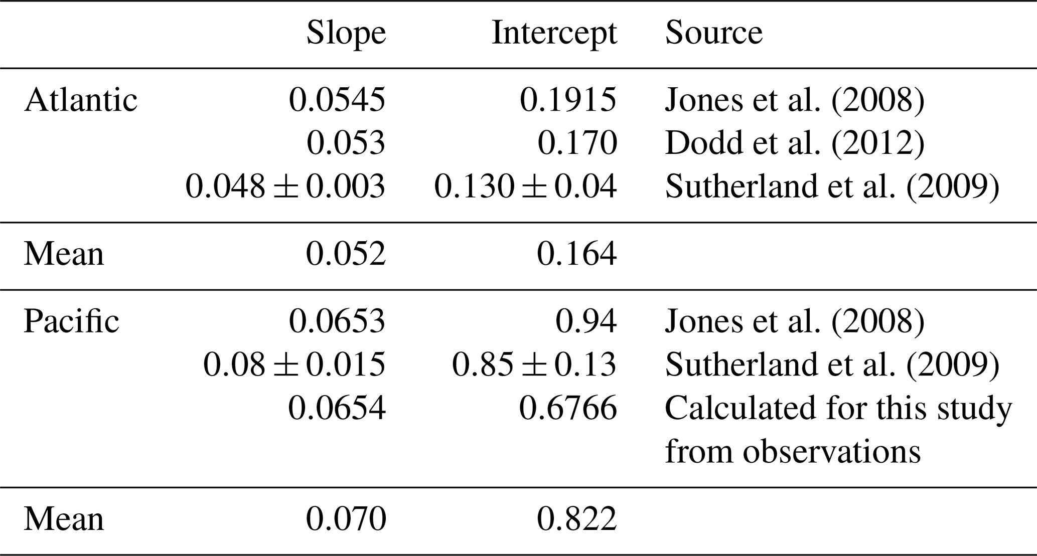
It is observed that Pacific seawater has higher relative concentrations of phosphate than Atlantic seawater (Bauch et al., 1995; Ekwurzel et al., 2001; Jones et al., 1998). Nitrate concentrations (used in combination with oxygen; Ekwurzel et al., 2001) are only quasi-conservative, as both are altered due to biological activity or air–sea exchange in surface waters (Alkire et al., 2015), while the use of nitrate : phosphate (N : P) nutrient ratios (Jones et al., 1998) has been considered to be conservative with respect to biological activity. However, there is emerging evidence that the N : P ratio may be becoming non-conservative in the Arctic Ocean as a consequence of sea ice retreat. Denitrification is a process that removes nitrogen from the biogeochemical system, and Bauch et al. (2011) and Alkire et al. (2019) both note that calculations based on the N : P ratio overestimate quantities of Pacific-derived seawaters as a result of denitrification of seawater in bottom sediments. Also, and despite the N : P ratios for the Atlantic and Pacific oceans exhibiting distinct linear relationships with near-constant slopes, there is variation in the exact form of this relationship (Jones et al., 2008; Sutherland et al., 2009; Dodd et al., 2012; Yamamoto-Kawai et al., 2008). In the Arctic Ocean, nutrient ratios have been used to trace the circulation of Pacific seawater (Jones et al., 1998; Jones, 2003), and to indicate the likely origins of freshwater sources (Yamamoto-Kawai et al., 2008; Sutherland et al., 2009).

Our aims in this study are (1) to generate new estimates of Arctic Ocean source fluxes using the geochemical approach, (2) to compare the results of the established budget approach to those of the new geochemical approach, and (3) to test the consistency of the various tracers used. To these ends, we first describe the data sources and the model used along with the attribution methods and schemes implemented (Sect. 2). Results are presented in Sect. 3, and discussed with an examination of the implications for the future use of biogeochemical tracers in the Arctic in Sect. 4.

2 Data and methods

2.1 Measurements

TB12 use an inverse model (Wunsch, 1978; Roemmich, 1980) that considers the Arctic Ocean as a control volume bounded by land and four gateways – Davis, Fram, and Bering straits and the Barents Sea Opening (Fig. 1) – and is divided into 15 horizontal layers defined by isopycnal surfaces. The TB12 inverse model generates an optimized horizontal velocity field v(s,z), where z is depth and s the along-boundary horizontal coordinate, which conserves volume and salinity transports, based on hydrographic data collected in summer 2005. For further details of the inverse model construction see TB12. For this study, the TB12 volume fluxes are combined with additional tracers to generate source component estimates of liquid Arctic freshwater fluxes, to compare with the existing net (salinity-derived) estimates of TB12.

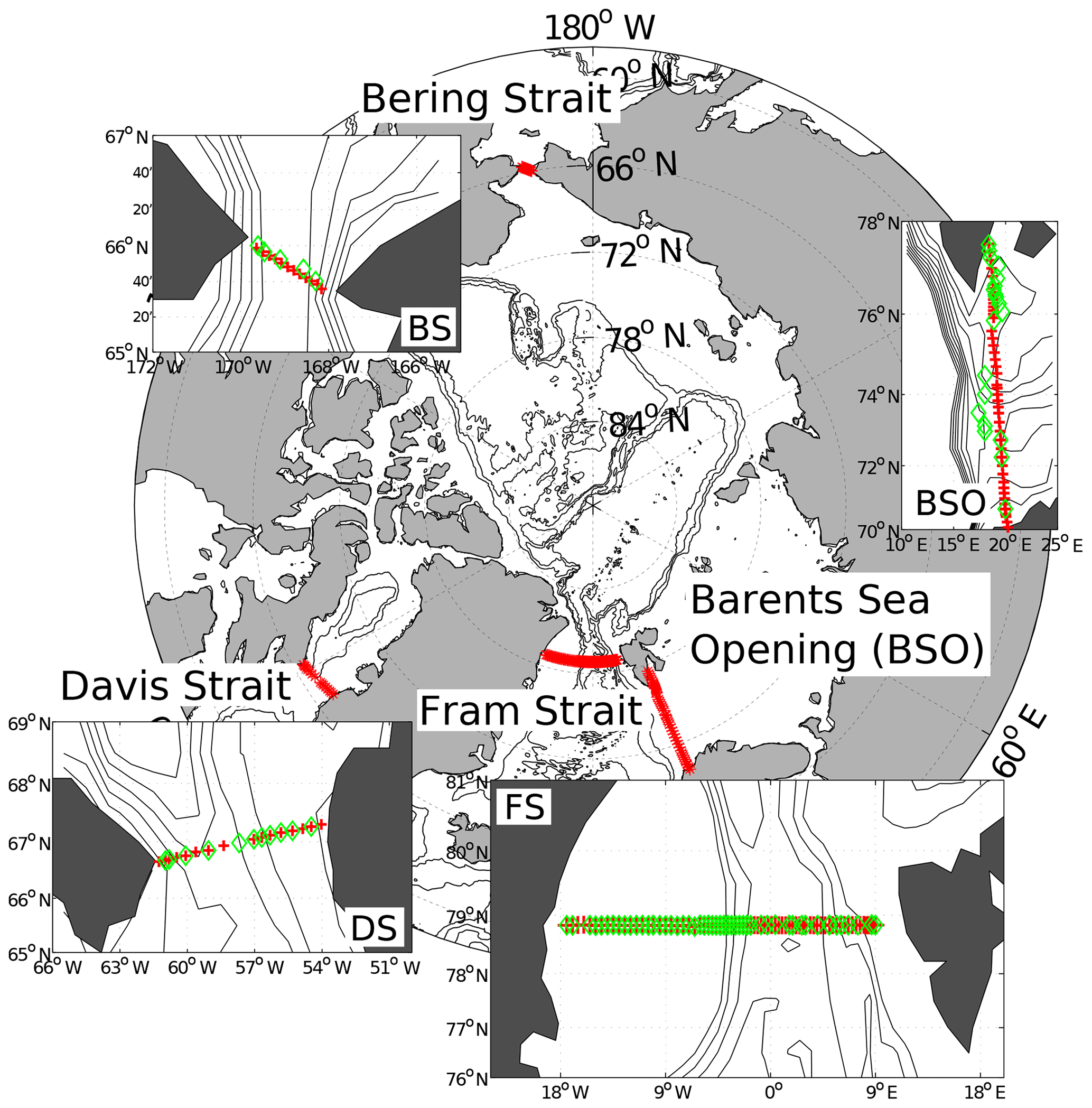
https://www.the-cryosphere.net/13/2111/2019/tc-13-2111-2019-f01

Figure 1Map of the Arctic Ocean, showing the four main gateways. The position of the δ¹⁸O and nutrient sample locations is indicated by green diamonds, and the Tsubouchi et al. (2012) CTD station positions by red crosses.

From the TB12 model, the Arctic boundary circulation is broadly conventional. Atlantic-origin seawater enters through the Barents Sea Opening with a volume flux of 3.6±1.1 Sv (± standard deviation). Pacific-origin seawater enters through Bering Strait with a volume flux of 1.0±0.2 Sv. Fram Strait is a net exporter of seawater, with a volume flux of 1.6±3.9 Sv, representing a balance between inflowing (mainly) Atlantic waters in the West Spitsbergen Current in the east of the strait (volume flux of 3.8±1.3 Sv) and outflowing waters in the East Greenland Current in the west of the strait (volume flux of 5.4±2.1 Sv). The net seawater export through Davis Strait has a volume flux of 3.1±0.7 Sv. For details of other relatively small contributions to the total, see TB12. As a simplified and approximate summary, ∼8 Sv of Atlantic-origin and ∼1 Sv of Pacific-origin seawater enters the Arctic, with ∼9 Sv of variously modified seawater exported. The net surface freshwater flux (both liquid and solid) calculated by TB12 is 187±44 mSv, 147±42 mSv in the liquid ocean plus 40±14 mSv in sea ice.

Biogeochemical data were originally collated and published by Torres-Valdés et al. (2013) for inorganic nutrients and MacGilchrist et al. (2014) for δ¹⁸O. Original datasets are described as follows. For Davis Strait see Lee et al. (2004) (with δ¹⁸O by Kumiko Azetsu-Scott, Department of Fisheries and Oceans, Bedford Institute of Oceanography). For Bering Strait see Woodgate et al. (2015). For the Barents Sea Opening see The International Council for the Exploration of the Sea Oceanographic Database (http://www.ices.dk/marine-data/dataset-collections/Pages/default.aspx, last access: 13 August 2019) for nutrient data, and Schmidt et al. (1999) for δ¹⁸O. For Fram Strait see Budéus et al. (2008) and Kattner (2011) for nutrient data, and Rabe et al. (2009) for δ¹⁸O. There are no δ¹⁸O measurements below ∼400 m in Fram Strait, so we simply extrapolate the deepest measurement to the bottom, for completeness. This depth is close to the Greenland–Scotland sill depths (600–800 m) to the south, so there is little or no net flux below these depths (TB12) and we do not expect the absence of deep δ¹⁸O to significantly impact our results. Sample locations are shown in Fig. 1.

Our domain comprises a total of 147 hydrographic stations, which includes data from 16 general circulation model grid cells in the Barents Sea Opening that are used as hydrographic stations, covering a total oceanic distance of 1803 km, with a total (vertical) section area of 1050 km². Vertical resolution is 1 dbar, with maximum pressures of 1044 dbar in Davis Strait, 2704 dbar in Fram Strait, 471 dbar in the Barents Sea Opening, and 52 dbar in Bering Strait (for further discussion of the model domain see TB12).

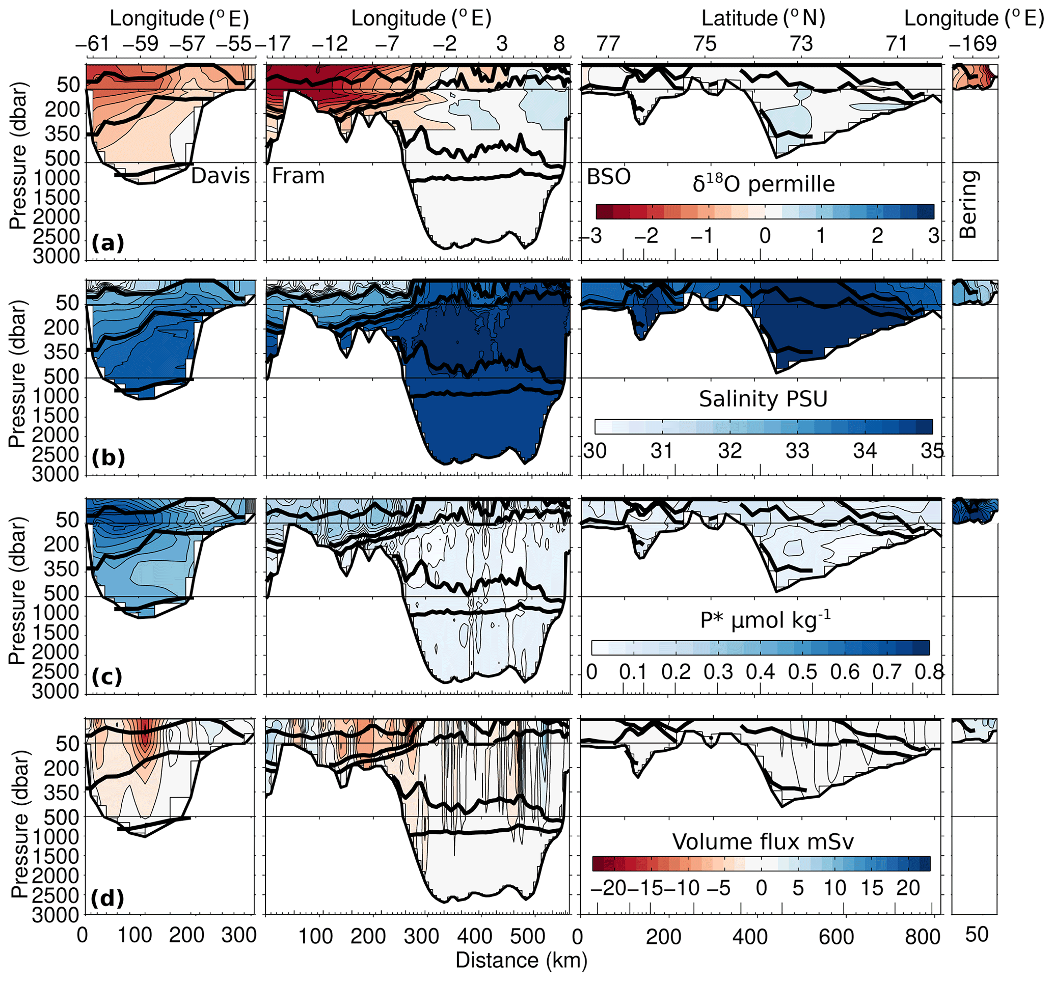
https://www.the-cryosphere.net/13/2111/2019/tc-13-2111-2019-f02

Figure 2Sections of δ¹⁸O (a), salinity (b), P^∗ (c) and volume flux from Tsubouchi et al. (2012) (d) after optimal interpolation onto the Tsubouchi et al. (2012) CTD station positions, clockwise around the four gateways from Davis Strait to Bering Strait. Solid black lines indicate the potential density (σ) surfaces separating the main Arctic water masses grouped as follows: surface water (σ₀<26.0), subsurface water ( $26.0 < σ_{0} < 27.1$ ), upper Atlantic water ( $27.1 < σ_{0} < 27.5$ ), Atlantic water (σ₀=27.5 to σ_0.5=30.28), intermediate water (σ_0.5=30.28 to σ₁=32.75) and deep water (σ₁>32.75); definitions from Tsubouchi et al. (2012). Note the broken scaling of the y axis.

The δ¹⁸O and nutrient data were optimally interpolated (Roemmich, 1983) vertically in pressure and horizontally in distance to match the TB12 model domain (Fig. 2). The interpolation recovers the measurements for each sample point and interpolates between values to fill the unsampled areas of the domain. The resulting nutrient fields show typical features, including low concentrations in the upper, sunlit layers as a consequence of nutrient utilization during primary production, and concentrations that increase with depth due to remineralization and/or dissolution of sinking particles; see also Torres-Valdés et al. (2013). The δ¹⁸O sample resolution is mainly adequate to capture the significant Arctic Ocean features, although in the Fram Strait section around 6^∘ W, there is only a single station to represent the East Greenland Current, so that horizontal gradients to either side of this station will only be approximate.

2.2 Approach

Following established practice, the sources of a parcel of oceanic water are considered to number three or four. The sources are characterized by end members, which are defined points in the phase space populated by the observed liquid (and solid i.e. sea ice) biogeochemical tracer properties, so that here “oceanic water” means the sum total of all liquid fractions. The term seawater is used to mean the typical source water fraction from the Atlantic (and also Pacific) Ocean; seawater fractions are always positive. The “meteoric” fraction can in principle be either positive, stemming directly or indirectly from rain- and snowfall, where the indirect route implies river runoff or terrestrial glacial input to the ocean, or negative, from evaporation. The “ice-modified” fraction is a result of sea ice freezing and melting, and (as will become apparent) appears mainly in oceanic water as negative fractions consequent on the freezing out of sea ice from oceanic water. For simplicity, therefore, we define this (negative) fraction as “brine”, following Östlund and Hut (1984), and use “sea ice meltwater” for the alternative (positive) case. Velocities into (out of) the Arctic Ocean are signed positive (negative), so that seawater imports (exports) are signed positive (negative), imports (exports) of positive fractions (rain, snow, rivers, etc.) of meteoric input are signed positive (negative) and brine imports (exports) are signed negative (positive).

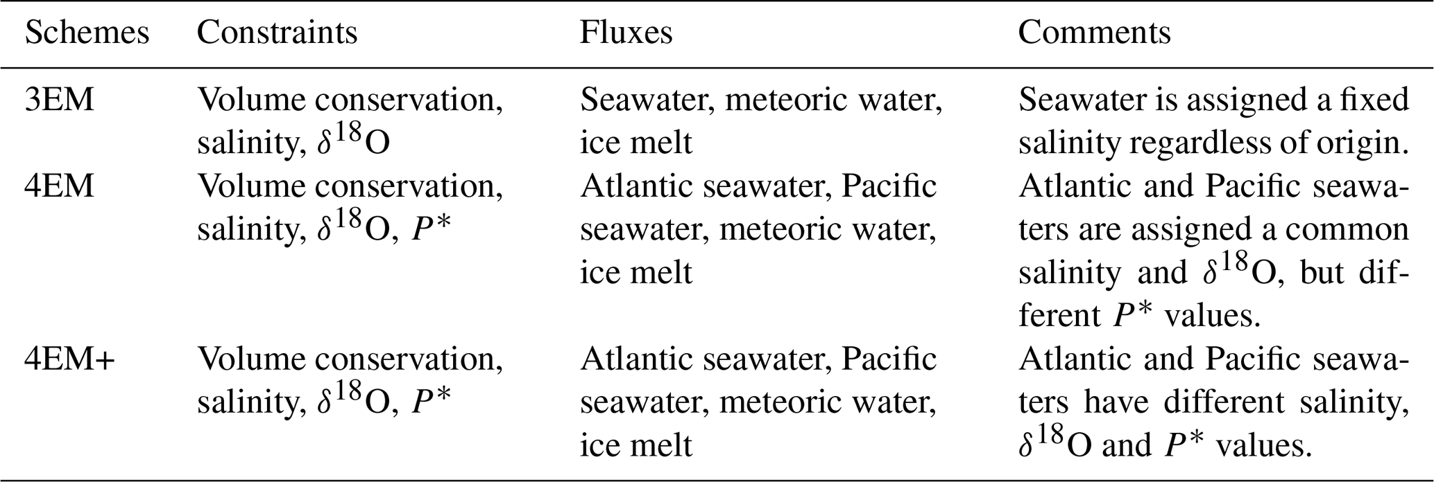
We employ three variants of the approach to the calculation of the resulting source fractions. Firstly a three-end-member scheme (3EM) is adopted, which uses salinity and δ¹⁸O to identify seawater, meteoric freshwater and ice-modified seawater (mainly brine). Secondly the 3EM scheme is extended to a four-end-member scheme (4EM) through the use of inorganic nutrient data, aiming to discriminate between seawater of Atlantic and Pacific origin, where the salinity and δ¹⁸O end-member properties of both ocean sources are assumed to be the same as for Atlantic seawater. Thirdly the 4EM scheme is applied again, but now adopting distinct end-member properties for both ocean-source salinity and δ¹⁸O (4EM+), replicating previous practice (Dodd et al., 2012; Jones et al., 2008; Sutherland et al., 2009). The properties of the three schemes are summarized in Table 1.

Table 1Description of the three model schemes.

Download Print Version | Download XLSX

To discriminate between Atlantic and Pacific seawaters, an additional relationship is formulated in terms of the concentrations of the inorganic nutrients phosphate and nitrate (Dodd et al., 2012; Jones et al., 1998). We form this relationship in terms of the variable P^∗, which is an expression describing the excess concentration of phosphate above that which would be expected from typical Redfield nutrient ratios (Redfield et al., 1963), and it employs the observed nitrate concentration

P^{*} = P_{m} - (N_{m} / 16),

where P_m and N_m are the measured nitrate and phosphate concentrations respectively. Atlantic and Pacific seawaters are each considered to have a distinct, near-constant nitrate-to-phosphate (N : P) ratio (Jones et al., 1998), which can be expressed algebraically as

P_{oce} = P_{slope} N_{m} + P_{int},

where P_oce is the estimated concentrations of phosphate from the relevant ocean (either Atlantic or Pacific) waters and the subscripts “slope” and “int” indicates the slope and intercept of the relationships. Boundary sections of salinity, δ¹⁸O and P^∗ are shown in Fig. 2.

To quantify source fractions for each oceanic water parcel (i.e. grid point), we establish the following system of equations. This problem is conventionally treated as “square”, with the number of constraints equal to the number of source water fractions to be determined for each water parcel. Each water parcel then has a suite of $i = 1, \dots, M$ measured properties x_i. Each measured property is treated as the sum of $j = 1, \dots, M$ fractions f_i of a suite of source properties X_i,j. The number of source properties (or end members) is M=3 or 4 here, and the associated freshwater sources are indicated as sea ice (j=1), meteoric (j=2), seawater (j=3 for 3EM), or Pacific and Atlantic seawater (j=3 and 4 for 4EM variants respectively). Written as a sum,

X_{i} = \sum_{j = 1}^{M} X_{i, j} f_{j} .

Setting all x, X=1 for i=1 retrieves the requirement that the sum of all the source fractions f_j accounts for all of the observed oceanic water:

\begin{matrix} (1) & 1 = \sum_{j = 1}^{M} f_{j} . \end{matrix}

The measured properties are then δ¹⁸O concentrations (i=2) and salinity (i=3) for all models; in addition the 4EM variants employ P^∗ for i=4 (Table 1). The product of this process is a system of M equations describing M unknowns, which is written in matrix form for (M×1) column vectors f and x, and (M×M) matrix X:

x = X f .

This is solved for f by standard (exact) inversion of a square matrix at each water parcel on our ocean boundary grid, to calculate the resulting spatial distributions of the relevant oceanic water source fractions:

f = X^{- 1} x .

2.3 End-member values

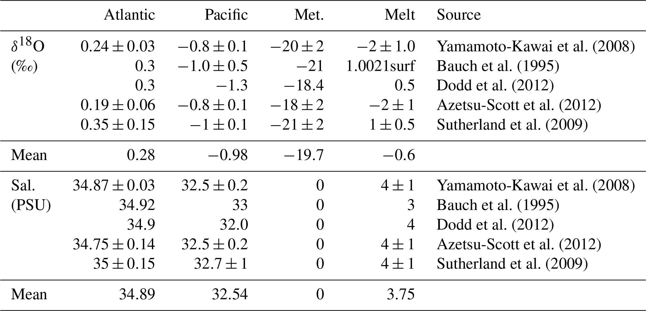
Previous studies have used different values for the end-member concentrations of salinity, δ¹⁸O and nutrients, which are summarized in Tables 2 and 3. A least-squares linear fit to the δ¹⁸O and salinity data from the three sections likely to contain freshwater of meteoric origin (Davis, Fram and Bering straits) suggests a δ¹⁸O end member in the range of −20 ‰ (Bering Strait) to −30 ‰ (Fram Strait), with a mean value of −23.3 ‰, which is within the range of the published values.

Yamamoto-Kawai et al. (2008)Bauch et al. (1995)Dodd et al. (2012)Azetsu-Scott et al. (2012)Sutherland et al. (2009)Yamamoto-Kawai et al. (2008)Bauch et al. (1995)Dodd et al. (2012)Azetsu-Scott et al. (2012)Sutherland et al. (2009)

Table 2End-member values for salinity and δ¹⁸O (‰) from the literature. Note Bauch et al. (1995) calculate ice melt δ¹⁸O by multiplying measured surface seawater δ¹⁸O(surf) by a “fractionation factor” of 1.0021.

Download Print Version | Download XLSX

Jones et al. (2008)Dodd et al. (2012)Sutherland et al. (2009)Jones et al. (2008)Sutherland et al. (2009)

Table 3P : N relationships, where ${PO}_{4} = slope \times {NO}_{3} + intercept$ (µmol kg⁻¹).

Download Print Version | Download XLSX

The relationships between salinity and δ¹⁸O for our data and from cited sources are shown in Fig. 3a. This phase diagram is akin to the oceanographer's “mixing diagram”, where measured oceanic water properties tend to lie along lines connecting core water mass properties as a result of mixing between those properties. In this case, processes that add sea ice meltwater or meteoric water cause mixing along the lines joining the three end points (seawater, meteoric water, sea ice meltwater). The difference here is that there are processes that remove water mass constituents (freezing, evaporation), and this is manifested on the phase diagram as points that “back away” from the relevant end points, clearly seen, for example, in Fig. 3a in the Fram Strait data. The Fram Strait data also exhibit the two-layer mixing relationship indicating the likely presence of Greenland ice sheet melt, which has a distinctly lighter δ¹⁸O signature (Cox et al., 2010). The fits to data from the three sections likely to contain Atlantic seawater (Fram and Davis straits, Barents Sea Opening) suggest an Atlantic seawater salinity end point of ≈35.

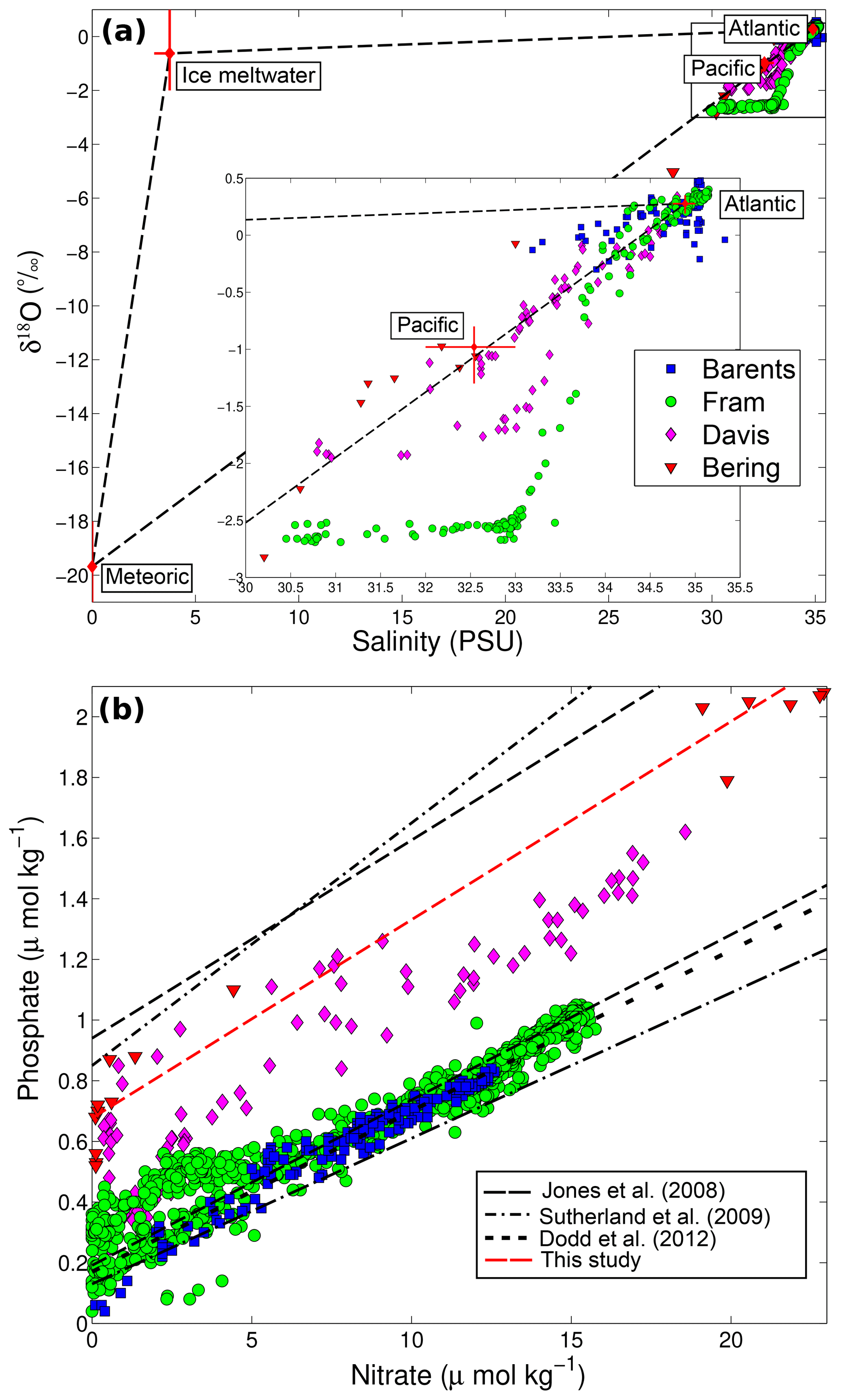
https://www.the-cryosphere.net/13/2111/2019/tc-13-2111-2019-f03

Figure 3(a) Salinity–δ¹⁸O relationship for all samples used in this paper; mean literature end points (± standard deviation) are marked. Red crosses indicate the mean values of literature end points and black dashed lines the mixing lines between them. (b) Nutrient data for all samples used in this paper compared to the published N : P relationships of Jones et al. (2008), Dodd et al. (2012) and Sutherland et al. (2009). The dashed red line indicates a best fit to the Bering Strait nutrient data presented here. Symbols denoting the data from each section are the same in both panels. Note Dodd et al. (2012) uses the same Pacific relationship as Jones et al. (2008).

Download

Considering the published nitrate–phosphate relationships, the most appropriate to this study are the values used by Jones et al. (2008), Sutherland et al. (2009) and Dodd et al. (2012) because Yamamoto-Kawai et al. (2008) include ammonium, and the nutrient measurements used here are of nitrate plus nitrite (Torres-Valdés et al., 2013). A least-squares best fit to the Bering Strait nutrient data has a slope of 0.0654, which is consistent with that of Jones et al. (2008), and an intercept of 0.6766 (Table 3). The relationships between nitrate and phosphate concentrations for our data and from cited sources are shown in Fig. 3b.

2.4 Freshwater flux calculation

We use the approach established by TB12 and developed by Bacon et al. (2015), which recognizes that a unique definition of a freshwater flux is given by the net surface exchange between the ocean (including ice) and the adjacent land and atmosphere, i.e. the net of precipitation, evaporation and runoff. The surface freshwater flux within an enclosed ocean volume is then calculated from its dilution effect on salinity:

F = ∯ \frac{v^{'} S^{'}}{\overline{S}} d s d z,

where the integral is taken around the ocean boundary, from seabed to surface, and including sea ice; the overbar indicates area mean and prime indicates deviation from the mean, i.e. $S = S^{'} + \overline{S}$ and $v = v^{'} + \overline{v}$ ; and s and z are horizontal and vertical coordinates respectively. TB12 describe the calculation and method in detail, and they also inspect the assumption of stationarity, concluding that, for a quasi-synoptic dataset such as this, it is justified (their Sect. 3.5).

Then in the stationary case the surface freshwater flux F is equal and opposite to the ice and ocean boundary volume transport V_O:

F + V_{O} = 0,

where

V_{O} = ∯ v (s, z) d s d z .

Lastly, the fraction of the ocean seawater flux per water parcel attributed to each n source, δV_O, is

δ V_{O, j} (s, z) = f_{i} (s, z) v (s, z) δ s δ z .

2.5 End-member uncertainty

Due to the wide range of plausible end-member values for each of the water types, to give an estimate of the likely uncertainty due to end-member choice, fluxes of the different water types were evaluated using a Monte Carlo technique. Distributions for the different end-member parameters were constructed from the cited values (Table 2) by assuming the parameter variability is normally distributed, with mean equal to the mean of the cited values and standard deviation equal to the range. A sample set of 1000 ensembles was drawn from the set of constructed parameter distributions using a Latin hypercube sampling strategy (McKay et al., 1979). The distributions of the individual parameters in the ensemble, which in all cases encompass the end points in Sect. 2.3 above, are shown in Fig. 4. Seawater salinity for 3EM and 4EM models is fixed at the boundary area mean salinity for the TB12 model (34.662). A second choice of seawater salinity end point (35.0) results from the discussion in Sect. 4.

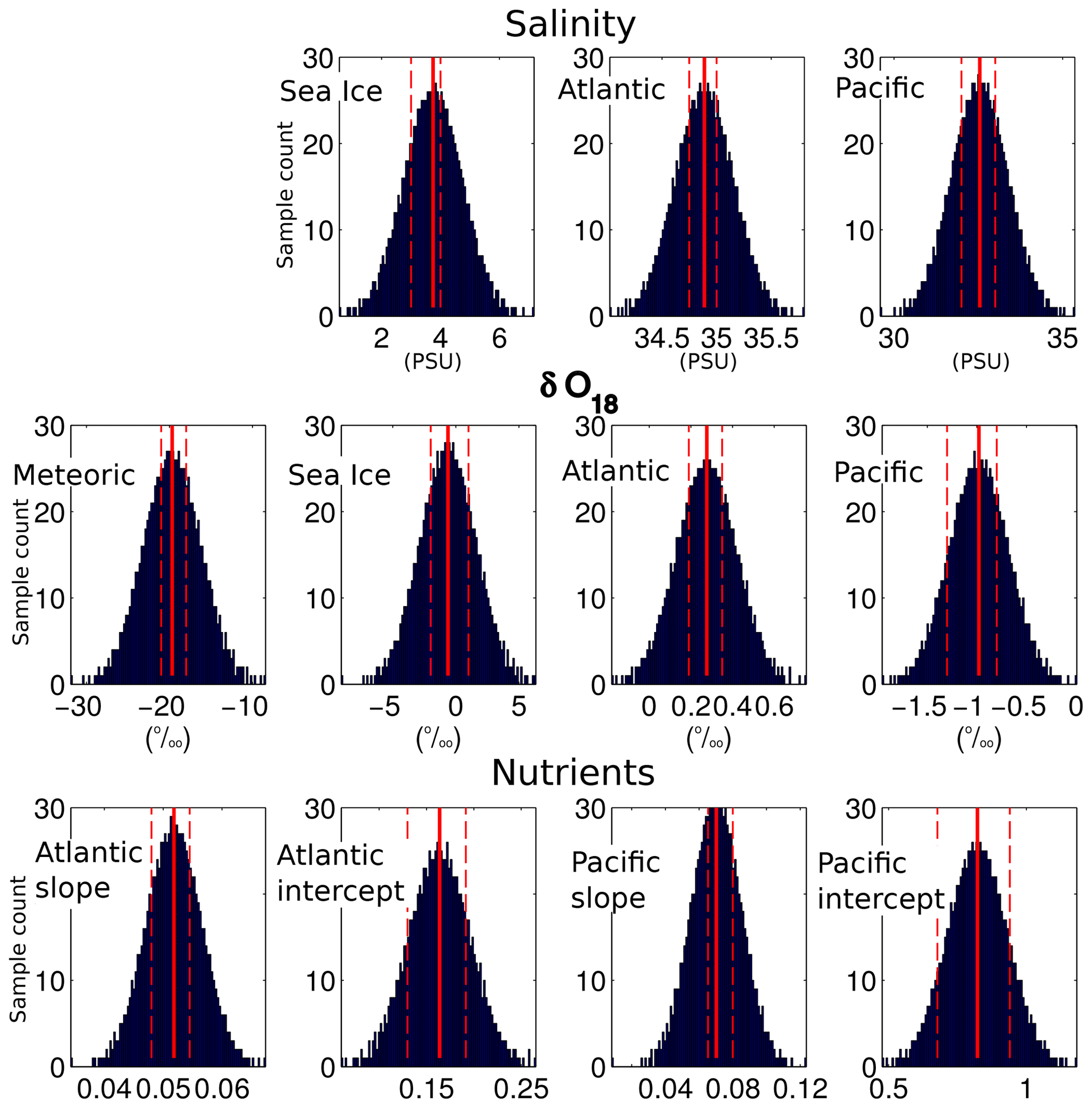
https://www.the-cryosphere.net/13/2111/2019/tc-13-2111-2019-f04

Figure 4Parameter space for the Monte Carlo simulations. Solid red line indicates the mean of the published values for the parameter; dashed red lines indicate maximum and minimum of published values.

Download

For each model approach, fluxes of the different water types were estimated by combining the velocities from the TB12 model with the calculated water type fractions for the sample ensemble. Mean and standard deviations for the attributed volume fluxes of each water type were calculated as the mean and standard deviation of the results from the sample ensemble.

3 Results

Here we present the results of the application of the methods and end members, described in Sect. 2, to generate three- and four-end-member freshwater source fractions and fluxes. Equation (1) allows for individual fractions to be either <0 or >1 as long as the sum of all fractions is equal to 1. Negative fractions of meteoric and ice-modified waters result from removal of freshwater from seawater by evaporation and sea ice formation respectively. However, seawater fractions, either total or individual Atlantic and Pacific water fractions, should be positive. Consequently, Pacific and Atlantic water fractions were made positive-definite by rounding to zero any of the fractions that were less than zero, and setting the remaining seawater fraction so that Eq. (1) was not invalidated.

3.1 Three-end-member model (3EM)

The distribution of 3EM source fractions is shown in Fig. 5. Ice-modified waters are found almost exclusively in the surface/upper waters of the model (depths down to 1000 dbar in the Davis Strait), with the highest-magnitude fractions (−0.15) found in subsurface waters of the western Fram Strait between depths of ∼50 and 300 dbar. The fractions of ice-modified waters are mostly negative, indicating brine, with a small fraction (∼0.05) being positive (indicating fresh meltwater input) in the surface (above 70 dbar) East Greenland Current (East Greenland Current; between 6.5 and 2^∘ W) of the Fram Strait. Meteoric waters are also found almost exclusively in the surface/upper waters of the model, with high fractions (>0.08) in the surface/subsurface waters (depths down to 350 dbar) in the Davis Strait and the western side of the Fram Strait. There is also a high fraction of meteoric water in the Bering Strait. Seawater fractions are high (∼1) in all deep and intermediate model waters at depths in excess of ∼350 dbar.

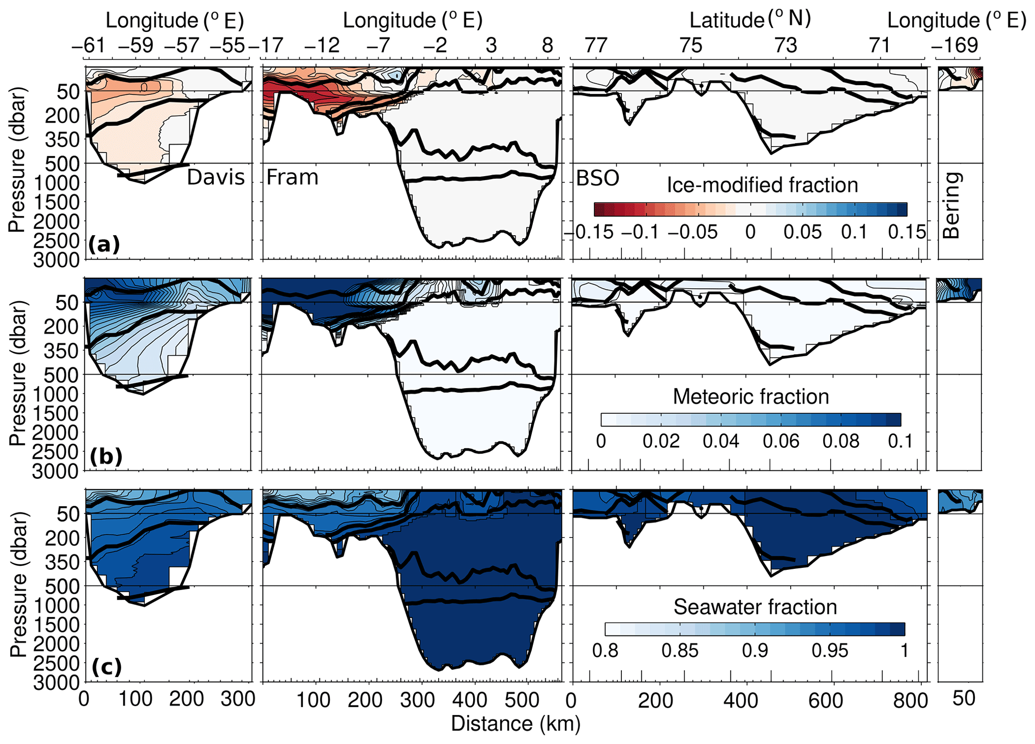
https://www.the-cryosphere.net/13/2111/2019/tc-13-2111-2019-f05

Figure 5Sections of ice-modified fraction (a), meteoric fraction (b) and seawater fraction (c), for the 3EM model, clockwise around the four gateways from Davis Strait to Bering Strait. Solid black lines indicate the isopycnal surfaces separating the main Arctic water masses as described in Tsubouchi et al. (2012). End members used were the mean of the literature values (see Tables 2 and 3). Note different colour scales for each panel.

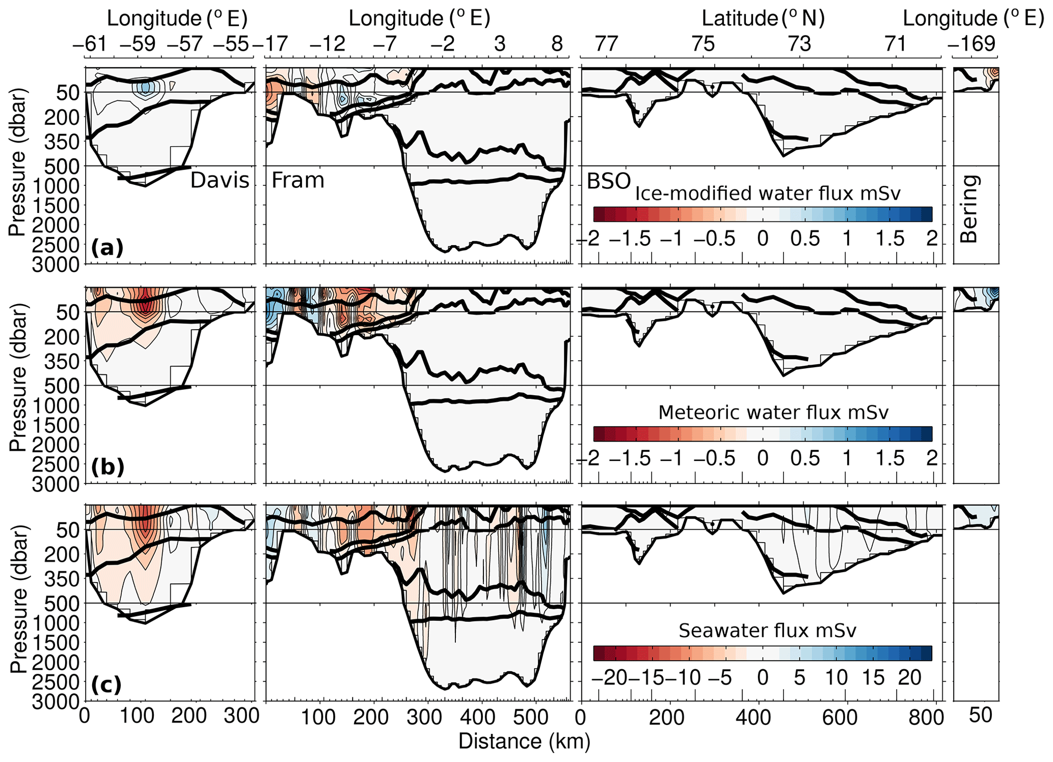
https://www.the-cryosphere.net/13/2111/2019/tc-13-2111-2019-f06

Figure 6Sections of ice-modified water flux (a), meteoric water flux (b) and seawater flux (c), for the 3EM model (mSv), clockwise around the four gateways from Davis Strait to Bering Strait. Solid black lines indicate the isopycnal surfaces separating the main Arctic water masses as described in Tsubouchi et al. (2012). End members used were the mean of the literature values (see Tables 2 and 3). Note different colour scales for each panel. Positive values indicate flux into the Arctic.

Typical volume fluxes (positive indicating into the Arctic) for the 3EM source fractions are shown in Fig. 6. The strongest fluxes of ice-modified waters occur as brine exports in surface waters of the middle of the Davis Strait and on the western side of the Fram Strait (East Greenland Current), and as brine import to the east in the Bering Strait, with fluxes of ∼0.1 Sv in magnitude. The patterns of countervailing fluxes over the Belgica Bank (west of 6.5^∘ W) in the Fram Strait indicate recirculation (see TB12). Meteoric water volume fluxes follow the same general pattern as for ice-modified waters, with strong export (∼0.1 Sv) in the middle of the Davis Strait and the East Greenland Current and strong import (∼0.1 Sv) of meteoric waters in the Bering Strait. Seawater volume fluxes resemble the oceanic circulation of TB12 (as expected), with concentrated exports in Davis Strait (∼1 Sv) and the East Greenland Current (∼0.5 Sv), and imports to the east in the Fram Strait in the West Spitsbergen Current (east of 5^∘ E) and in the Bering Strait.

Table 4Mean volume fluxes (Sv ± standard deviation) for the three-end-member (3EM) model. Positive values indicate fluxes into the Arctic. Values of solid freshwater flux from Tsubouchi et al. (2012).

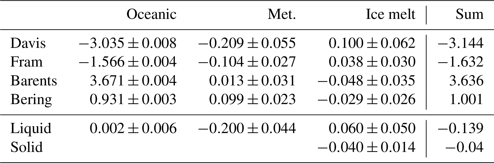
Download Print Version | Download XLSX

For the 3EM model schemes, the net seawater volume flux is effectively zero (0.002±0.006 Sv, Table 4, Monte Carlo uncertainty quantification). The net volume export of meteoric waters (200±44 mSv) is consistent with the TB12 surface freshwater input of 187±44 mSv (Table 4). The model also indicates a net brine input export (60±50 mSv), which is similar to the model solid sea ice export of 40±14 mSv, with the bulk of the brine export occurring through the Davis Strait (Table 4).

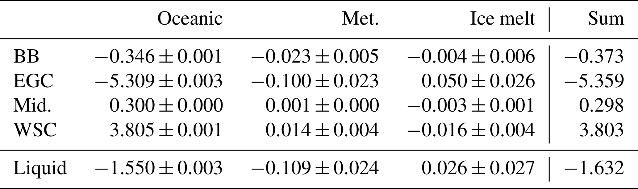
Table 5Mean volume fluxes (Sv ± standard deviation) for the components of the Fram Strait flux (Belgica Bank, BB; East Greenland Current, EGC; mid-strait, Mid.; West Spitsbergen Current, WSC) from the three-end-member (3EM) model. Positive values indicate fluxes into the Arctic.

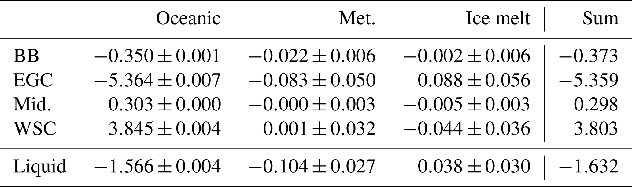
Download Print Version | Download XLSX

The 3EM model indicates that the volume export of meteoric water through Fram Strait is concentrated in the Belgica Bank and East Greenland Current regions, 22±6 and 83±50 mSv respectively, with close to zero meteoric flux in the remainder of the strait (Table 5). This is consistent with the picture described in previous studies: Dodd et al. (2012), Rabe et al. (2009) and Meredith et al. (2001). Brine is exported mainly in the East Greenland Current (88±56 mSv), with small (∼5 mSv) fluxes of ice-modified water in the middle and Belgica Bank sections of the strait (Table 5). The apparent brine import in both the West Spitsbergen Current and the Barents Sea Opening, 44±36 mSv (Table 4) 48±35 mSv (Table 5) respectively, reflects the higher δ¹⁸O values at the surface (∼0.4 ‰) relative to those for deeper waters (∼0.2 ‰)) to the east of 5^∘ W (Fig. 2). This is discussed in Sect. 4.

3.2 Four-end-member models (4EM and 4EM+)

The 4EM scheme extends the 3EM scheme through use of inorganic nutrient (nitrate and phosphate) data, aiming to discriminate between Atlantic and Pacific seawater origin. The 4EM scheme retains single end points for salinity and δ¹⁸O, as in 3EM. In the 4EM+ scheme, distinct salinity and δ¹⁸O end-member properties are attributed to Atlantic and Pacific seawaters, replicating previous practice (Dodd et al., 2012; Jones et al., 2008; Sutherland et al., 2009). The resulting distributions of 4EM and 4EM+ source fractions are shown in Figs. 7 and 9 respectively, and characteristic volume fluxes for the source fractions in Figs. 8 and 10.

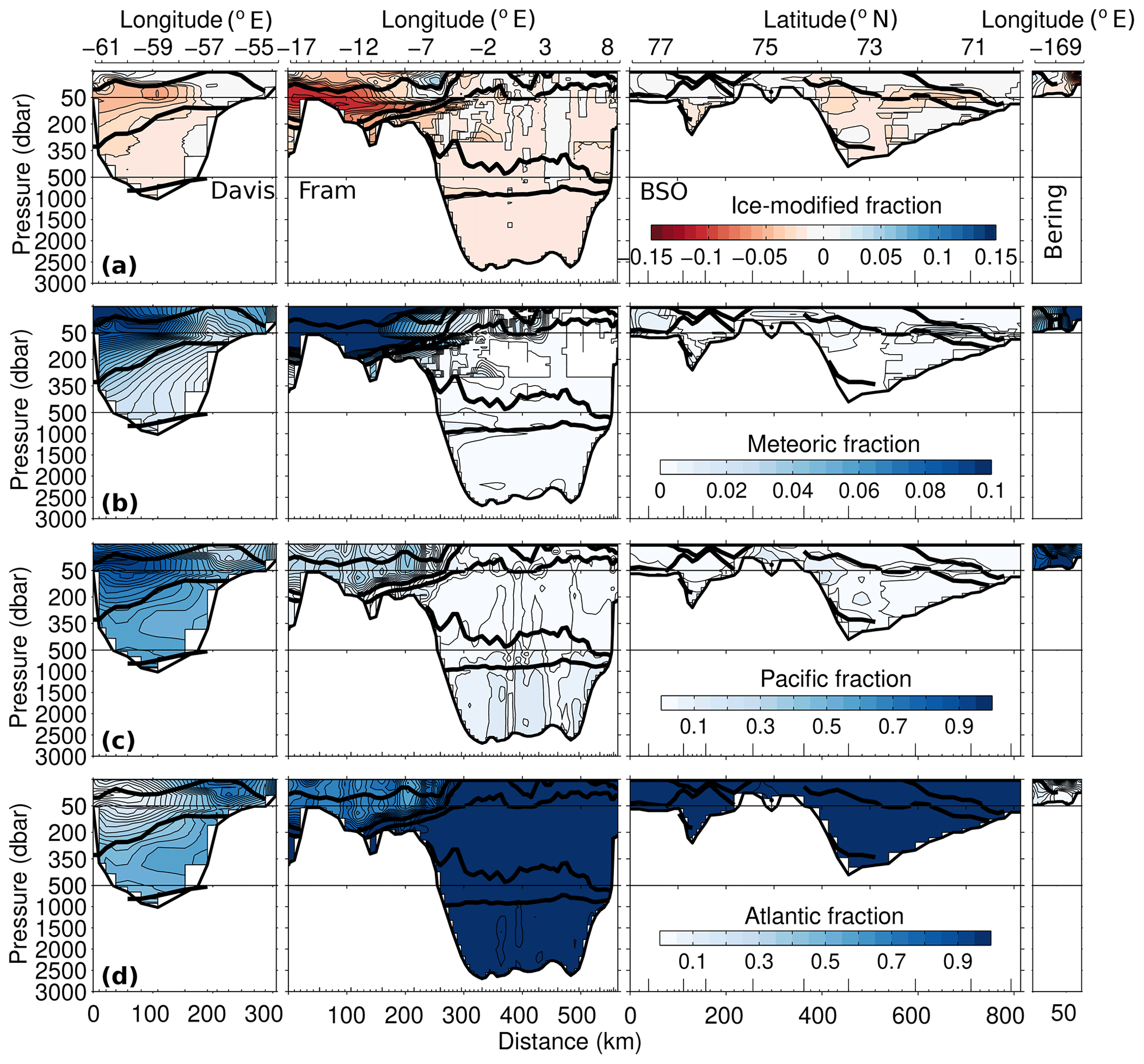
https://www.the-cryosphere.net/13/2111/2019/tc-13-2111-2019-f07

Figure 7Sections of ice-modified fraction (a), meteoric fraction (b), Pacific fraction (c) and Atlantic fraction (d), for the 4EM model, clockwise around the four gateways from Davis Strait to Bering Strait. Solid black lines indicate the isopycnal surfaces separating the main Arctic water masses as described in Tsubouchi et al. (2012). End members used were the mean of the literature values (see Tables 2 and 3). Note different colour scales for each panel.

https://www.the-cryosphere.net/13/2111/2019/tc-13-2111-2019-f08

Figure 8Sections of ice-modified water flux (a), meteoric water flux (b), Pacific water flux (c) and Atlantic water flux (d), for the 4EM model (mSv), clockwise around the four gateways from Davis Strait to Bering Strait. Solid black lines indicate the isopycnal surfaces separating the main Arctic water masses as described in Tsubouchi et al. (2012). End members used were the mean of the literature values (see Tables 2 and 3). Note different colour scales for each panel. Positive values indicate flux into the Arctic.

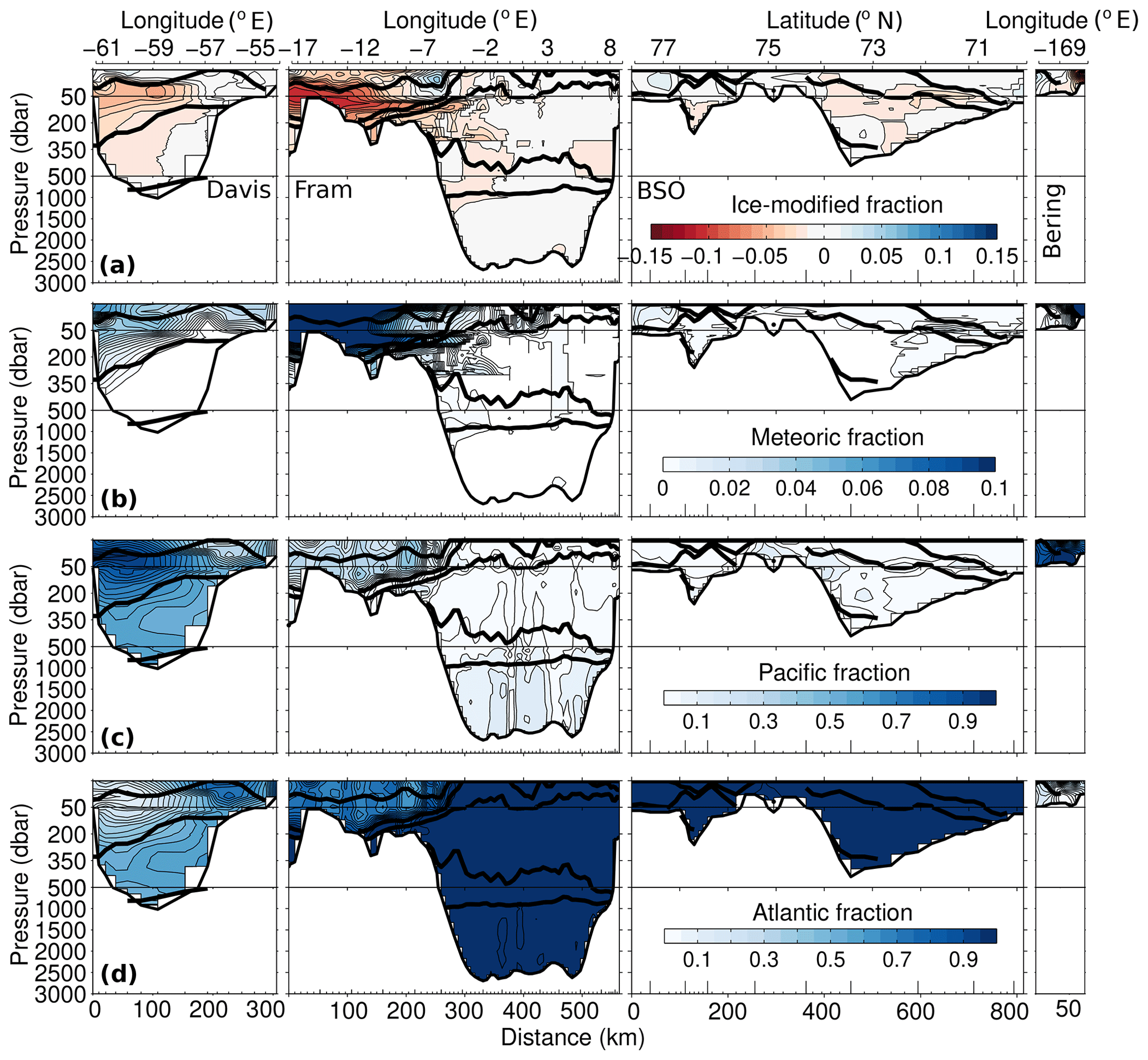
https://www.the-cryosphere.net/13/2111/2019/tc-13-2111-2019-f09

Figure 9Sections of ice-modified fraction (a), meteoric fraction (b), Pacific fraction (c) and Atlantic fraction (d), for the 4EM+ model, clockwise around the four gateways from Davis Strait to Bering Strait. Solid black lines indicate the isopycnal surfaces separating the main Arctic water masses as described in Tsubouchi et al. (2012). End members used were the mean of the literature values (see Tables 2 and 3). Note different colour scales for each panel.

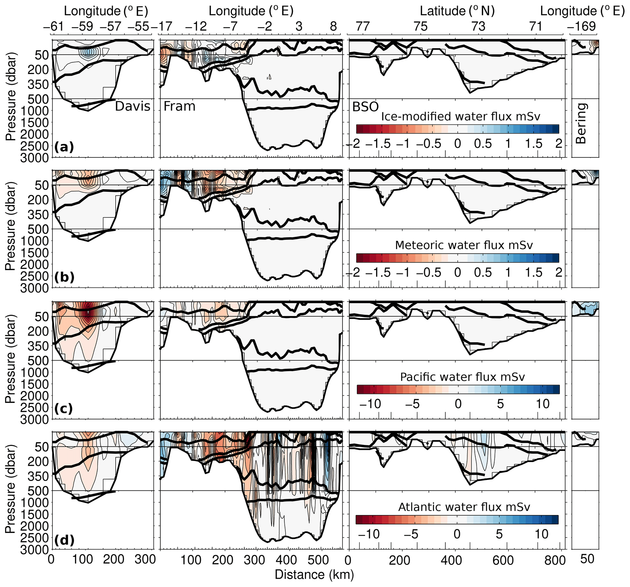
https://www.the-cryosphere.net/13/2111/2019/tc-13-2111-2019-f10

Figure 10Sections of ice-modified water flux (a), meteoric water flux (b), Pacific water flux (c) and Atlantic water flux (d), for the 4EM+ model (mSv), clockwise around the four gateways from Davis Strait to Bering Strait. Solid black lines indicate the isopycnal surfaces separating the main Arctic water masses as described in Tsubouchi et al. (2012). End members used were the mean of the literature values (see Tables 2 and 3). Note different colour scales for each panel. Positive values indicate flux into the Arctic.

Similar to the 3EM model, both 4EM and 4EM+ models allocate the bulk of the ice-modified waters, mainly brine with some meltwater input, to the surface/upper waters. However, both four-end-member schemes indicate small but non-zero fractions (∼0.01) of brine in the east of the Fram Strait and in the Barents Sea Opening. The distribution of meteoric waters in both four-end-member models is consistent with the 3EM model where meteoric waters also mostly occupy the surface layers. However, differences occur in the Davis Strait, where the 4EM and 4EM+ models indicate lower fractions (∼0.01) below ∼350 dbar, in the Bering Strait where meteoric water is confined to the eastern side and in the deeper waters of the model where the meteoric fraction is non-zero (<0.01). Both four-end-member models indicate Pacific water mostly in the surface/near-surface waters of the Davis, Fram and Bering straits, and almost exclusively Atlantic water in the deepest waters of the model (∼0.9). Both models show small fractions of Pacific water in the deep waters of the Fram Strait and Barents Sea Opening (∼0.1) and Atlantic water in the Bering Strait (∼0.1).

Table 6Mean volume fluxes (Sv ± standard deviation) for the four-end-member (4EM) model. Positive values indicate fluxes into the Arctic. Values of solid freshwater flux from Tsubouchi et al. (2012).

Download Print Version | Download XLSX

Differences between the three- and four-end-member model schemes are also reflected in the fluxes of the different fractions. For both four-end-member models, there are non-zero fluxes of brine, meteoric water (both <0.005 Sv) and Pacific water (<0.02 Sv) in the deeper waters of the Fram Strait and Barents Sea Opening. Consistent with the 3EM model, the 4EM model has a net oceanic volume flux (sum of Pacific and Atlantic contributions) that is effectively zero (4EM 0.002±0.006 Sv, Table 6), but the net oceanic volume flux for the 4EM+ model is non-zero indicating a net export ( $- 0.104 \pm 0.051$ Sv, Table 8). Net model liquid freshwater export (sum of meteoric and ice-modified fractions) for the 4EM model is the same as for the 3EM model (140±67 mSv), while the 4EM+ export is smaller with a large relative uncertainty (35±51 mSv).

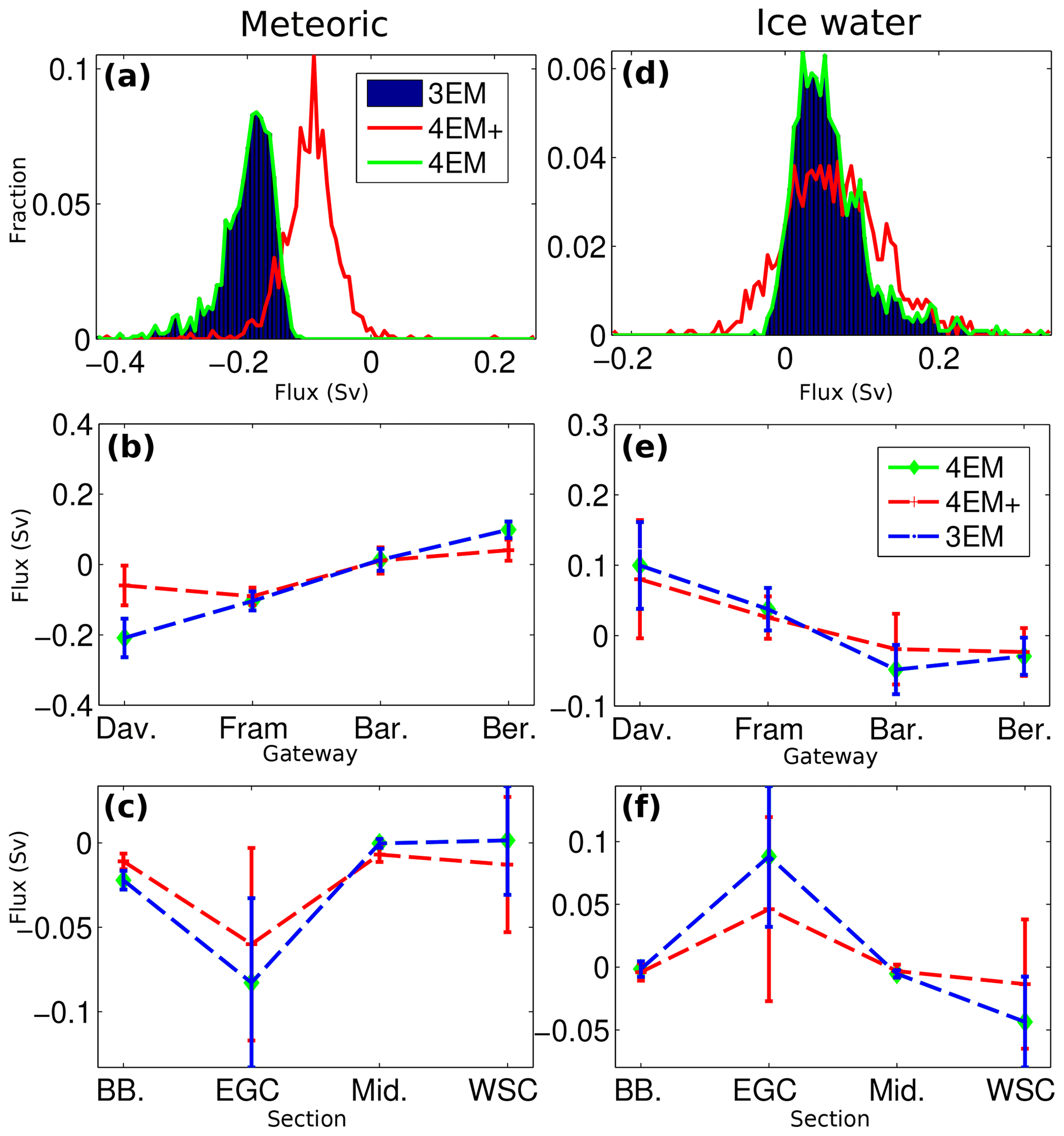
https://www.the-cryosphere.net/13/2111/2019/tc-13-2111-2019-f11

Figure 11Meteoric and ice water volume fluxes. (a, d) Histograms of the total attributed volume fluxes (Sv) for all model schemes. (b, e) Mean volume fluxes (Sv ± standard deviation) for each gateway. (c, f) Volume fluxes (Sv ± standard deviation) for the components of the Fram Strait (Belgica Bank, BB; East Greenland Current, EGC; mid-strait, Mid.; West Spitsbergen Current, WSC). The 3EM model is in blue, the 4EM model in green, and the 4EM+ model in red. Positive values indicate fluxes into the Arctic.

Download

The net ice-modified water (mainly brine) flux for both the 4EM and 4EM+ schemes is also consistent with the 3EM model and the TB12 solid ice flux, with the 4EM model estimating 60±50 mSv and the 4EM+ 63±64 mSv (Tables 6 and 8). Both 4EM and 4EM+ models show the same flux pattern for ice-modified water as the 3EM model, with the bulk of the brine input exiting through the Davis Strait (Tables 4, 6 and 8, Fig. 11).

While the net volume flux of meteoric water for the 4EM model is the same as that of the 3EM (200±44 mSv), the 4EM+ model estimates a smaller net volume flux (98±46 mSv, Tables 6 and 8). Both 4EM and 4EM+ models show the same flux pattern for meteoric water as the 3EM model, with meteoric water entering the Bering Strait and exiting through the Davis and Fram straits. However, the net import of meteoric water through the Bering Strait and the net export of meteoric water through the Davis Strait in the 4EM+ model schemes is approximately half the magnitude of the fluxes in the other two schemes (Tables 4, 6 and 8, Fig. 11).

Both 4EM and 4EM+ model schemes indicate an imbalance in the net volume fluxes for both Pacific and Atlantic water. They both show a net export of Pacific water (4EM 1.495±0.268 Sv; 4EM+ 1.488±0.263 Sv) that is balanced by a net import of Atlantic water of approximately equal magnitude (4EM 1.497±0.268 Sv; 4EM+ 1.384±0.255 Sv, Tables 6 and 8). Current understanding of Arctic fluxes suggests that Pacific water enters the Bering Strait and exits both through the Davis Strait, after passing through the western Canadian Archipelago, and on the western side of the Fram Strait (Haine et al., 2015). Consistent with this view, both four-end-member schemes indicate that Pacific water, entering the Arctic through the Bering Strait, exits mostly through the Davis Strait with a much (O(10×)) smaller flux through the Fram Strait, mainly across Belgica Bank and in the East Greenland Current. Export of Pacific water through the Davis Strait is approximately twice the magnitude of the import through the Bering Strait (Tables 6 and 8). Atlantic water circulates in through the Barents Sea Opening and out through the western Fram and Davis straits, with the import through the Barents Sea Opening approximately twice the magnitude of the export (Tables 6 and 8).

Table 7Mean volume fluxes (Sv ± standard deviation) for the components of the Fram Strait flux (Belgica Bank, BB; East Greenland Current, EGC; mid-strait, Mid.; West Spitsbergen Current, WSC) from the four-end-member (4EM) model. Positive values indicate fluxes into the Arctic.

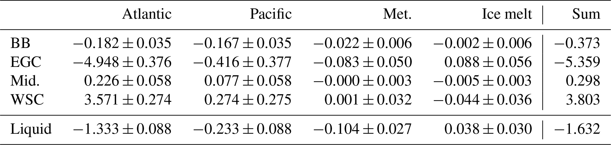
Download Print Version | Download XLSX

Table 8Mean volume fluxes (Sv ± standard deviation) for the four-end-member (4EM+) model. Positive values indicate fluxes into the Arctic. Values of solid freshwater flux from Tsubouchi et al. (2012).

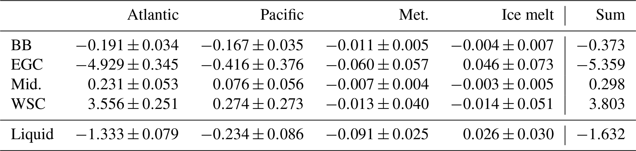
Download Print Version | Download XLSX

Table 9Mean volume fluxes (Sv ± standard deviation) for the components of the Fram Strait flux (Belgica Bank, BB; East Greenland Current, EGC; mid-strait, Mid.; West Spitsbergen Current, WSC) from the four-end-member (4EM+) model. Positive values indicate fluxes into the Arctic.

Download Print Version | Download XLSX

For the Fram Strait, the pattern of water fluxes described by both the 4EM and 4EM+ schemes is consistent with the pattern described above for the 3EM model (Tables 7 and 9). In both four-end-member schemes, Pacific water is exported across Belgica Bank and in the East Greenland Current, accounting for approximately 15 % of the Fram Strait oceanic volume flux (Tables 7 and 9). While fluxes of meteoric and ice-modified waters described by the 4EM model are the same as for the 3EM model (Table 7), the fluxes from the 4EM+ schemes are different (Table 9).

The description of Arctic freshwater fluxes presented by the 4EM+ model is broadly consistent with that from previous studies of fluxes in the Fram Strait using 4EM+ type schemes with distinct Pacific seawater, δ¹⁸O and salinity end members (Dodd et al., 2012; Azetsu-Scott et al., 2012; Rabe et al., 2013). Analysis of a time series of observations from the Fram Strait suggests a mean freshwater export flux dominated by waters of meteoric origin, mixed with brine to the west of 2^∘ W in the East Greenland Current and over the Greenland shelf (Belgica Bank), with fluxes of negative meteoric origin waters also noted in the West Spitsbergen Current (Dodd et al., 2012; Rabe et al., 2013).

The greatest differences between the models are in the fluxes of meteoric, brine and ice meltwaters across Belgica Bank and in the East Greenland Current (Fig. 11), with the 4EM+ schemes showing less export of meteoric water in the East Greenland Current compared to the other schemes. In the 4EM+ model, the import of high-salinity water in the West Spitsbergen Current is attributed almost equally to negative meteoric origin water and high-salinity ice-modified (brine input) water, in contrast to the 4EM and 3EM schemes, which attribute this high-salinity import to brine (Tables 7 and 9). Brine export is also lower in the 4EM+ schemes compared to the 3EM and 4EM models (Tables 7 and 9; Fig. 11).

In the Davis Strait the 4EM+ model is qualitatively consistent with previous studies, where source fractions show the highest freshwater content in the surface waters on the western side of the strait, from Pacific seawater and meteoric fractions, with a contribution from brine (Azetsu-Scott et al., 2012). To the east of the Davis Strait, there is a small contribution from sea ice meltwater (Azetsu-Scott et al., 2012).

4 Discussion and summary

Within uncertainty, the net seawater flux of the 3EM and 4EM models is zero: 2±6 mSv for 3EM and 2±379 mSv for 4EM (Tables 4 and 6). Thus in this section, we first discuss the “minority” water mass constituents, meaning ice-modified waters (mainly brine), and Pacific waters and meteoric waters, in terms of implications for net fluxes and fundamental points of interpretation; finally, we offer some general perspectives.

4.1 Ice-modified waters

The models generate apparent brine imports in the West Spitsbergen Current and the Barents Sea Opening, both with magnitude of ∼45 mSv and a total of ∼90 mSv with a large relative uncertainty of ∼50 mSv. If correct, this is a substantial component of the Arctic Ocean freshwater budget. These (apparent) fluxes are too small to be visible in Fig. 5, but for scale, note that each net (oceanic water) inflow is ∼3 Sv, 1 % of which is 30 mSv. These brine fluxes are consequences of weakly positive δ¹⁸O anomalies centred around ∼300 m depth in both locations, each about 200 m thick and each spanning ∼200 km. The presence of these features in both Fram Strait and the Barents Sea Opening suggests that they are source water (Atlantic seawater) properties and not the result of modifications by local processes. Frew et al. (2000) examine the oxygen isotope composition of northern North Atlantic water masses from measurements made in 1991. Considering the waters of interest here – the upper ∼500 m in the eastern North Atlantic (their stations 10, 24, 26, 72) – we find (broadly) salinities and δ¹⁸O values in the ranges 35.0–35.2 and 0.2–0.4 ‰ respectively (their Fig. 2). This combination and range describes the part of the dense cloud of points heading a short distance north-eastwards in phase space away from the seawater end point (Fig. 3 panel a inset).

Table 10Mean volume fluxes (Sv ± standard deviation) for a three-end-member model with seawater salinity and δ¹⁸O fixed at 35.0 and 0.35 ‰ respectively. Positive values indicate fluxes into the Arctic. Values of solid freshwater flux from Tsubouchi et al. (2012).

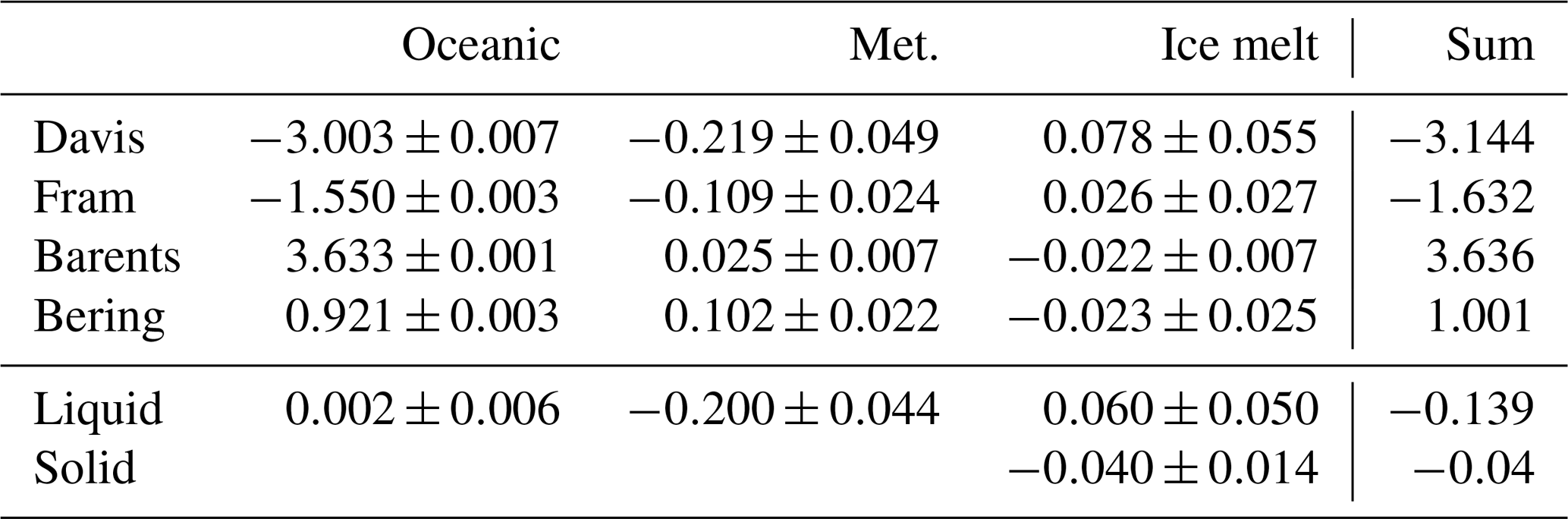
Download Print Version | Download XLSX

Table 11Mean volume fluxes (Sv ± standard deviation) for the components of the Fram Strait flux (Belgica Bank, BB; East Greenland Current, EGC; mid-strait, Mid.; West Spitsbergen Current, WSC) for a three-end-member model with seawater salinity and δ¹⁸O fixed at 35.0 and 0.35 ‰ respectively. Positive values indicate fluxes into the Arctic.

Download Print Version | Download XLSX

A consistent interpretation of the apparent West Spitsbergen Current and Barents Sea Opening brine imports, therefore, is that they are actually manifestations not of local processes but rather of source water variability, in the light of our salinity (34.662) and δ¹⁸O (mean 0.2 ‰) end points. As a result, we ran the 3EM model again, now with salinity of 35.0 and fixed δ¹⁸O of 0.35 ‰; the results are shown in Tables 10 and 11. There is no change to component totals (seawater, brine, meteoric totals), or to gateway totals (Fram, Davis and Bering straits, and the Barents Sea Opening), but there are significant component changes between gateways and within Fram Strait. For the Barents Sea Opening, we see 38 mSv removed from the seawater component and added to the meteoric fraction, approximately doubling the meteoric freshwater import from 13±31 to 25±7 mSv, more than halving the ice-modified water flux, which we have been interpreting as brine import, from 48±35 to 22±7 mSv, and greatly reducing their uncertainties (1 SD), giving us confidence that this new 3EM run is better in this regard. The two freshwater import values are consistent with freshwater entering the Arctic Ocean in the Norwegian Coastal Current as the 14 mSv of TB12, who use a boundary mean salinity (effective) reference of 34.67, and with the 23 mSv of Smedsrud et al. (2010), using a salinity reference of 35.0, as for our new 3EM run respectively. The remaining 22 mSv of ice-modified water is, therefore, unlikely to be brine import, given the δ¹⁸O mean end point of 0.35 ‰; it is more likely to be meltwater export south of Svalbard (see Gammelsrød et al., 2009). A similar pattern is seen in the West Spitsbergen Current in the east of Fram Strait, where an apparent brine import and its uncertainty of 44±36 mSv decrease to 16±4 mSv. For our geochemical approach, we began with a salinity end point that replicated the budget method's effective salinity reference value; however, we conclude that the geochemical approach requires a different geochemical salinity end point, relevant to the source water properties under consideration. At the same time, there must be some uncertainty associated with the seawater end point properties, even when considering only the Atlantic source, given the measurements of Frew et al. (2000), given that their measurements were made 14 years before those used here and given that we lack more evidence of upstream (source) δ¹⁸O variability.

A second point concerns the near-total absence of positive ice-modified fractions, representing sea ice melt, anywhere around the boundary (Fig. 5). The actual absence of melted sea ice in late summer in these locations is not credible. However, inspection of the two Arctic export routes west and east of Greenland – Davis Strait and the East Greenland Current (in the west of Fram Strait) – shows similar features: high brine fractions around 50 m depth, decreasing towards the surface. In common with Cox et al. (2010), we interpret this as the result of sea melting back into the oceanic water from which it (partly) originated, resulting in (partial) reduction of the brine signal.

Thirdly, we know that sea ice is frozen out of liquid seawater, and it leaves behind in the seawater a negative δ¹⁸O signal resulting from this distillation-type process (Östlund and Hut, 1984). In the long-term mean, and allowing for trends in net freshwater input and lags between this input at the surface and its manifestation at the boundary, the positive freshwater export flux of the sea ice should be approximately equal to the negative freshwater (brine) export flux. We find a surprising coincidence (allowing for uncertainties) between the net brine flux, at 60±50 mSv for both the 3EM and 4EM models, and the TB12 sea ice export of 40±14 mSv. More work is needed to understand how representative this balance may be; for example, would wintertime measurements of sea ice and brine fluxes show a similar balance? What does this say about the influence of local versus non-local freeze-out and melt-back processes on seasonal brine and sea ice export variability?

4.2 Pacific water

The only change in the 4EM model over 3EM is the inclusion of P^∗, intended to distinguish seawater of Atlantic origin from that of Pacific origin. The retention of single salinity and δ¹⁸O end points for seawater ensures that all source water fluxes remain the same as for 3EM apart from the separation of seawater into Atlantic- and Pacific-sourced fluxes (Tables 6 and 7). In the 4EM model, ∼1 Sv of Pacific seawater enters the Arctic through Bering Strait, while more than double that – ∼2.5 Sv – of Pacific seawater exits the Arctic, mainly through Davis Strait, indicating the apparent net “creation” of ∼1.5 Sv of Pacific seawater (Table 6). This is mirrored by the origins and fate of Atlantic seawater, with ∼3.6 Sv entering the Arctic and only ∼2.1 Sv exiting, indicating an apparent net “destruction” of ∼1.5 Sv of Atlantic seawater (Table 6). The magnitude of this apparent “conversion” of Atlantic to Pacific seawater is over 5 times greater than the uncertainty on the fluxes (∼0.3 Sv; Table 6). This apparent conversion of 1.5 Sv of Atlantic to Pacific water is outside any plausible uncertainty of the relevant volume and nutrient fluxes; see TB12 and Torres-Valdés et al. (2013). Furthermore, it is similar to TB12's downward export of 1.9 Sv out of the Atlantic water layer into denser layers.

The distribution of the 4EM Pacific fraction around the Arctic Ocean boundary (Fig. 5) shows the expected geographical distribution, with the main concentrations in the Bering Strait (import) and Davis Strait (export) and weaker concentrations in the west of Fram Strait (export). Not previously reported, however, are significant concentrations at depth (fractions ≥0.1 at depths ≥500 m) across Fram Strait. A credible hypothesis to explain all these observations – the doubling of Pacific export over import, the transformation of Atlantic water and the deep presence of Pacific water – concerns denitrification, the process that occurs in ocean sediments and removes nitrate from the ecosystem by discharging N₂. Chang and Devol (2009) estimate a net pan-Arctic denitrification rate of ∼13 Tg N yr⁻¹, with much of that expected to occur in the shallow waters of the Barents and Chukchi seas (6 and 3 Tg N yr⁻¹ respectively). They further note the likelihood that the process is a consequence of sea ice retreat enabling increased primary production through increased shelf-break upwelling, which delivers nutrient-rich waters to upper-ocean waters with greater light availability; the resulting increase in export production then fuels higher rates of sedimentary denitrification. In addition, and while the geographical distribution and intensity of circum-Arctic dense water formation remains an active topic of research, it is known that the wintertime Barents Sea supports significant dense water formation rates and that the dense product waters exit the Barents Sea via St. Anna Trough (e.g. Aksenov et al., 2010). Thus there exists a credible mechanism to denitrify inflowing Atlantic water and then to transmit it into the deep Arctic Ocean.

We acknowledge that much remains unknown about the Arctic Ocean biogeochemical cycle; understanding of denitrification is at an early stage, and understanding of Arctic Ocean sources and sinks of nitrate and phosphate is incomplete (Chang and Devol, 2009; Alkire et al., 2019; Bauch et al., 2011; Torres-Valdés et al., 2016). The N : P nutrient ratio of river runoff has been pragmatically assumed to be constant and to match that of Atlantic seawater, in that it has no phosphate excess (Dodd et al., 2012; Yamamoto-Kawai et al., 2008; Jones et al., 2008), and knowledge of the riverine delivery of nutrients is less well constrained than estimates of freshwater volume (Bring et al., 2016, 2017). Nevertheless, the N : P ratio (expressed here as P^∗) was proposed as a tracer that would be conservative with respect to biological activity (Jones et al., 1998, 2008; Yamamoto-Kawai et al., 2008). The results presented here, when combined with those of Bauch et al. (2011) and Alkire et al. (2019), strongly suggest that the N : P ratio is no longer conservative. We suggest, however, that it may still be useful in generating net quantification of denitrification rates, once the question of sources and sinks is resolved. For illustration, using an Atlantic-to-Pacific nitrate offset of 5–10 µ mol L⁻¹ (Fig. 3) and a water mass conversion rate of 1.5 Sv (as above), we find a net apparent pan-Arctic denitrification rate of 3.3–6.6 Tg N yr⁻¹, the same order of magnitude as the 13 Tg N yr⁻¹ of Chang and Devol (2009), but including Baffin Bay, which they do not.

Another inconsistency arises from consideration of results from the 4EM+ model (Tables 8 and 9), when Pacific and Atlantic seawaters are defined as separate categories using both salinity and δ¹⁸O. These two seawaters will lie on the mixing line between any single seawater end point and pure freshwater (Fig. 3). If Pacific seawater lies on this mixing line and is also defined as a separate category, then these constraints are degenerate. This is reflected in the significant shifts of fluxes between all components – Atlantic, Pacific, meteoric and ice-related.

4.3 Meteoric water

A primary positive result of this study is the finding that both variants of the 3EM model (and the 4EM model) robustly quantify the net rate of Arctic meteoric freshwater input (the net of $P - E + R$ within the defined boundary) as 200±44 mSv (Tables 4, 6, 10), and that this geochemical quantification agrees closely with the TB12 budget method net surface freshwater input rate (within the same boundary) of 187±44 mSv, providing a degree of cross-validation of both methods.

An inconsistency arises from consideration of the composition and “labelling” of the waters of Bering Strait. Water entering the Arctic through the Bering Strait should, by definition, be seawater of Pacific origin. However, the Bering Strait inflow is unusually fresh because it contains a significant fraction of meteoric freshwater (Östlund and Hut, 1984, and Table 4), originating in part from the Alaskan Coastal Current on the east side of Bering Strait, which preserves the runoff signal from the western North American rivers (e.g. Woodgate and Aagaard, 2005; Chan et al., 2011). A second reason for the presence of meteoric freshwater in Bering Strait is the basic fact that the Pacific Ocean experiences a net positive precipitation anomaly (e.g. Warren, 1983). There are therefore two sets of constraints on the water in Bering Strait: it must be all Pacific water (defined by P^∗) because that is where it comes from, and it must be ∼10 % meteoric freshwater (defined by δ¹⁸O) to generate its low salinity. These constraints must, therefore, be partially degenerate (Fig. 3).

The results of using at least partially degenerate constraints on the model fluxes are most clearly manifested in the 4EM+ model. The models with single seawater end point values (3EM and 4EM) have near-zero net seawater export (actually 2±6 mSv), while the 4EM+ model shows a positive net seawater export (as the sum of Atlantic and Pacific seawaters) of 104±51 mSv, which mainly occurs in Davis Strait. At the same time, the meteoric water export flux is about half that of the 4EM model (Tables 6 and 8), with the difference appearing (again) mainly in Davis Strait. The model is balancing reduced meteoric freshwater export with increased salinity export, and it is able to do that because Atlantic seawater, Pacific seawater and meteoric freshwater all lie on the same mixing line: the degeneracy causes unrealistic results.

4.4 Perspectives

Our geochemical approach to oceanic water flux calculation employs three valid and geochemically distinct categories of water: sea ice (in its various manifestations), meteoric (surface-origin) freshwater and seawater (where seawater is the component of the mixture that contains all of the dissolved salts). First, we note again that our total sea ice flux, being the sum of the fluxes of solid sea ice, sea ice meltwater and the freshwater deficit (brine) in the seawater from which the ice was formed, is approximately zero. Second, the TB12 velocity field is constrained to conserve salinity, and this is reflected in our zero net seawater fluxes, which is another statement of salinity conservation because seawater is the category that contains all of the ocean salinity. Third, we note that the same categories (both here and in TB12) of surface-origin freshwater are all meteoric, as the net of $P - E + R$ . This is why our surface (meteoric) freshwater flux agrees with the TB12 results: both are (explicitly or implicitly) meteoric.

We find the category Pacific water, defined from the N : P ratio, to be non-conservative; however, it is very likely to continue to be useful, probably to quantify pan-Arctic denitrification, possibly also to help quantify dense water formation rates, where that process happens in denitrifying shelf seas. This continuing – albeit different – usefulness of the N : P ratio relies on retention of single salinity and δ¹⁸O end points to describe seawater, so that the N : P categorization can then only operate on seawater. Degeneracy intrudes with subdivision of salinity and δ¹⁸O categories, meaning that three would-be end points (Atlantic, Pacific, meteoric) actually lie on the same salinity–δ¹⁸O mixing line, causing confused results, for both the Atlantic–Pacific contrast and the Pacific–meteoric contrast.

In terms of δ¹⁸O signal, precipitation–evaporation and freezing–melting are manifestations of the same process with opposite signs. Consequently, δ¹⁸O values reflecting only net isotopic fractionation are unable to quantify river runoff without the use of another conservative tracer. It was hoped that barium could be used as a tracer of riverine input into the Arctic (Kenison Falkner et al., 1994). However, barium was found to be non-conservative (through biological scavenging) in seawater (Abrahamsen et al., 2009). Nevertheless, other more exotic species may prove useful. For instance, Laukert et al. (2017) show that the distribution of neodymium isotopes in Fram Strait bears a considerable resemblance to our Pacific water distribution (our Fig. 9, their Fig. 3), and with a similar interpretation to ours (Sect. 4.2 above) for the provenance of the water mass. Furthermore, Wefing et al. (2019) analyse isotopes of iodine and uranium, sourced from UK and French nuclear reprocessing plants, which trace Arctic Ocean circulation pathways and residence times, showing that some fraction of the near-surface freshened oceanic waters in the west of Fram Strait, which appear to be of Pacific origin from the N : P analysis, may actually have originated from the Norwegian Coastal Current.

We envisage that sustained measurement of suitable tracers around the Arctic boundary has the potential to further our quantification and understanding of key processes, variability, and timescales and to help mitigate the scarcity of observations in the Arctic Ocean interior. More (and more reliable) tracers are needed, more observations of more traditional tracers are needed through the water column (from surface to sea bed), more of those observations are needed in seasons outside summer and autumn, and we need better understanding of Arctic Ocean biogeochemical processes.

Data availability

All data used in the analysis presented here are available from the original authors. See Sect. 2.1 for details.

Author contributions

AF conducted the analysis and prepared the paper. SB, ACNG and STV assisted with the analysis and preparation of the paper. TT and STV assembled the data used, and TT assisted with the analysis.

Competing interests

The authors declare that they have no conflict of interest.

Acknowledgements

Alberto C. Naveira Garabato acknowledges the support of the Royal Society and the Wolfson Foundation.

Financial support

This study was funded by the U.K. Natural Environment Research Council as a contribution to the TEA-COSI (The Environment of the Arctic Climate, Ocean and Sea Ice) project grant no. NE/I028947/1.

Review statement

This paper was edited by Christian Haas and reviewed by Thomas Armitage and Wilken-Jon von Appen.

References

Aagaard, K. and Carmack, E. C.: The role of sea ice and other fresh water in the Arctic circulation, J. Geophys. Res.-Oceans, 94, 14485–14498, 1989. a, b

Abrahamsen, E. P., Meredith, M. P., Falkner, K. K., Torres-Valdes, S., Leng, M. J., Alkire, M. B., Bacon, S., Laxon, S. W., Polyakov, I., and Ivanov, V.: Tracer-derived freshwater composition of the Siberian continental shelf and slope following the extreme Arctic summer of 2007, Geophys. Res. Lett., 36, L07602, https://doi.org/10.1029/2009GL037341, 2009. a

Aksenov, Y., Bacon, S., Coward, A. C., and Holliday, N. P.: Polar outflow from the Arctic Ocean: A high resolution model study, J. Marine Syst., 83, 14–37, https://doi.org/10.1016/j.jmarsys.2010.06.007, 2010. a

Aleksandrov, Y. I., Bryazgin, N. N., Førland, E. J., Radionov, V. F., and Svyashchennikov, P. N.: Seasonal, interannual and long-term variability of precipitation and snow depth in the region of the Barents and Kara seas, Polar Res., 24, 69–85, https://doi.org/10.3402/polar.v24i1.6254, 2005. a

Alkire, M. B., Morison, J., and Andersen, R.: Variability in the meteoric water, sea-ice melt, and Pacific water contributions to the central Arctic Ocean, 2000-2014, J. Geophys. Res.-Oceans, 120, 1573–1598, https://doi.org/10.1002/2014JC010023, 2015. a

Alkire, M. B., Rember, R., and Polyakov, I.: Discrepancy in the Identification of the Atlantic/Pacific Front in the Central Arctic Ocean: NO Versus Nutrient Relationships, Geophys. Res. Lett., 46, 3843–3852, https://doi.org/10.1029/2018GL081837, 2019. a, b, c

Azetsu-Scott, K., Petrie, B., Yeats, P., and Lee, C.: Composition and fluxes of freshwater through Davis Strait using multiple chemical tracers, J. Geophys. Res., 117, C12011, https://doi.org/10.1029/2012JC008172, 2012. a, b, c, d, e

Bacon, S., Aksenov, Y., Fawcett, S., and Madec, G.: Arctic mass, freshwater and heat fluxes: methods and modelled seasonal variability, Philos. T. Roy. Soc. A, 373, 20140169, https://doi.org/10.1098/rsta.2014.0169, 2015. a, b

Bauch, D., Schlosser, P., and Faribanks, R. G.: Freshwater balance and the sources of deep and bottom waters in the Arctic Ocean inferred from the distribution of H218O, Prog. Oceanogr., 35, 53–80, 1995. a, b, c, d, e

Bauch, D., van der Loeff, M. R., Andersen, N., Torres-Valdes, S., Bakker, K., and Abrahamsen, E. P.: Origin of freshwater and polynya water in the Arctic Ocean halocline in summer 2007, Prog. Oceanogr., 91, 482–495, https://doi.org/10.1016/j.pocean.2011.07.017, 2011. a, b, c

Bring, A., Fedorova, I., Dibike, Y., Hinzman, L., Mård, J., Mernild, S. H., Prowse, T., Semenova, O., Stuefer, S. L., and Woo, M.-K.: Arctic terrestrial hydrology: A synthesis of processes, regional effects, and research challenges, J. Geophys. Res.-Biogeo., 121, 621–649, https://doi.org/10.1002/2015JG003131, 2016. a, b, c

Bring, A., Shiklomanov, A., and Lammers, R. B.: Pan-Arctic river discharge: Prioritizing monitoring of future climate change hot spots, Earth's Future, 5, 72–92, https://doi.org/10.1002/2016EF000434, 2017. a, b

Budéus, G., Fahrbach, E., and Lemke, P.: The Expedition ARKTIS-XXI/1 a and b of the Research Vessel Polarstern in 2005., Tech. rep., Alfred Wegener Institute for Polar and Marine Research, Bremerhaven, https://doi.org/10.2312/BzPM_0570_2008, 2008. a

Carmack, E. C., Yamamoto-Kawai, M., Haine, T. W. N., Bacon, S., Bluhm, B. A., Lique, C., Melling, H., Polyakov, I. V., Straneo, F., Timmermans, M.-L., and Williams, W. J.: Freshwater and its role in the Arctic Marine System: Sources, disposition, storage, export, and physical and biogeochemical consequences in the Arctic and global oceans, J. Geophys. Res.-Biogeo., 121, 675–717, https://doi.org/10.1002/2015JG003140, 2016. a, b, c, d

Chan, P., Halfar, J., Williams, B., Hetzinger, S., Steneck, R., Zack, T., and Jacob, D. E.: Freshening of the Alaska Coastal Current recorded by coralline algal Ba/Ca ratios, J. Geophys. Res.-Biogeo., 116, G01032, https://doi.org/10.1029/2010JG001548, 2011. a

Chang, B. X. and Devol, A. H.: Seasonal and spatial patterns of sedimentary denitrification rates in the Chukchi sea, Deep-Sea Res. Pt. II, 56, 1339–1350, https://doi.org/10.1016/j.dsr2.2008.10.024, 2009. a, b, c

Cox, K. A., Stanford, J. D., McVicar, A. J., Rohling, E. J., Heywood, K. J., Bacon, S., Bolshaw, M., Dodd, P. A., De la Rosa, S., and Wilkinson, D.: Interannual variability of Arctic sea ice export into the East Greenland Current, J. Geophys. Res.-Oceans, 115, C12063, https://doi.org/10.1029/2010JC006227, 2010. a, b, c, d

Craig, H.: Isotopic Variations in Meteoric Waters, Science, 133, 1702–1703, 1961. a

Dickson, R., Rudels, B., Dye, S., Karcher, M., Meincke, J., and Yashayaev, I.: Current estimates of freshwater flux through Arctic and subarctic seas, Prog. Oceanogr., 73, 210–230, https://doi.org/10.1016/j.pocean.2006.12.003, 2007. a, b, c

Dodd, P. A., Rabe, B., Hansen, E., Falck, E., Mackensen, A., Rohling, E., Stedmon, C., and Kristiansen, S.: The freshwater composition of the Fram Strait outflow derived from a decade of tracer measurements, J. Geophys. Res., 117, C11005, https://doi.org/10.1029/2012JC008011, 2012. a, b, c, d, e, f, g, h, i, j, k, l, m, n, o

Ekwurzel, B., Schlosser, P., Mortlock, R. A., Fairbanks, R. G., and Swift, J. H.: River runoff, sea ice meltwater, and Pacific water distribution and mean residence times in the Arctic Ocean, J. Geophys. Res.-Oceans, 106, 9075–9092, https://doi.org/10.1029/1999JC000024, 2001. a, b

Francis, J. A. and Vavrus, S. J.: Evidence linking Arctic amplification to extreme weather in mid-latitudes, Geophys. Res. Lett., 39, L06801, https://doi.org/10.1029/2012GL051000, 2012. a

Frew, R. D., Dennis, P. F., Heywood, K. J., Meredith, M. P., and Boswell, S. M.: The oxygen isotope composition of water masses in the northern North Atlantic, Deep-Sea Res. Pt. I, 47, 2265–2286, https://doi.org/10.1016/S0967-0637(00)00023-6, 2000. a, b

Gammelsrød, T., Leikvin, Ø., Lien, V., Budgell, W. P., Loeng, H., and Maslowski, W.: Mass and heat transports in the NE Barents Sea: Observations and models, J. Marine Syst., 75, 56–69, https://doi.org/10.1016/j.jmarsys.2008.07.010, 2009. a

Haine, T. W. N., Curry, B., Gerdes, R., Hansen, E., Karcher, M., Lee, C., Rudels, B., Spreen, G., de Steur, L., Stewart, K. D., and Woodgate, R.: Arctic freshwater export: Status, mechanisms, and prospects, Global Planet. Change, 125, 13–35, https://doi.org/10.1016/j.gloplacha.2014.11.013, 2015. a, b, c, d

Jones, E. P.: Tracing Pacific water in the North Atlantic Ocean, J. Geophys. Res., 108, 3116, https://doi.org/10.1029/2001JC001141, 2003. a

Jones, E. P., Anderson, L. G., and Swift, J. H.: Distribution of Atlantic and pacific waters in the upper Arctic Ocean: Implications for circulation, Geophys. Res. Lett., 25, 765–768, 1998. a, b, c, d, e, f

Jones, E. P., Anderson, L. G., Jutterström, S., Mintrop, L., and Swift, J. H.: Pacific freshwater, river water and sea ice meltwater across Arctic Ocean basins: Results from the 2005 Beringia Expedition, J. Geophys. Res., 113, C08012, https://doi.org/10.1029/2007JC004124, 2008. a, b, c, d, e, f, g, h, i, j, k

Kattner, G.: Inorganic nutrients measured on water bottle samples during POLARSTERN cruise ARK-XXI/1. PANGAEA, https://doi.org/10.1594/PANGAEA.761684, 2011. a

Kenison Falkner, K., Macdonald, R. W., Carmack, E. C., and Weingartner, T.: The Potential of Barium as a Tracer of Arctic Water Masses, in: The Polar Oceans and Their Role in Shaping the Global Environment, edited by: Johannessen, O. M., Muench, R. D., and Overland, J. E., American Geophysical Union, 63–76, https://doi.org/10.1029/GM085p0063, 1994. a

Lammers, R. B., Pundsack, J. W., and Shiklomanov, A. I.: Variability in river temperature, discharge, and energy flux from the Russian pan-Arctic landmass, J. Geophys. Res.-Biogeo., 112, G04S59, https://doi.org/10.1029/2006JG000370, 2007. a

Laukert, G., Frank, M., Bauch, D., Hathorne, E. C., Rabe, B., von Appen, W.-J., Wegner, C., Zieringer, M., and Kassens, H.: Ocean circulation and freshwater pathways in the Arctic Mediterranean based on a combined Nd isotope, REE and oxygen isotope section across Fram Strait, Geochim. Cosmochim. Ac., 202, 285–309, https://doi.org/10.1016/j.gca.2016.12.028, 2017. a

Lee, C. M., Abriel, J., Gabat, J. I., Petrie, B., Scotney, M., Soukhovtsev, V., and Thiel, K. V.: An Observational Array for High-Resolution, Year-Round Measurements of Volume, Freshwater, and Ice Flux Variability in Davis Strait: Cruise Report for R/V Knorr 179-05, 22 September–4 October 2004, Tech. rep., Univ. of Washington, Seattle, WA, USA, 2004. a

Lique, C., Holland, M. M., Dibike, Y. B., Lawrence, D. M., and Screen, J. A.: Modeling the Arctic freshwater system and its integration in the global system: Lessons learned and future challenges, J. Geophys. Res.-Biogeo., 121, 540–566, https://doi.org/10.1002/2015JG003120, 2016. a, b

MacGilchrist, G., Naveira Garabato, A., Tsubouchi, T., Bacon, S., Torres-Valdés, S., and Azetsu-Scott, K.: The Arctic Ocean carbon sink, Deep-Sea Res. Pt. I, 86, 39–55, https://doi.org/10.1016/j.dsr.2014.01.002, 2014. a

Manabe, S. and Stouffer, R. J.: Simulation of abrupt climate change induced by freshwater input to the North Atlantic Ocean, Nature, 378, 165–167, https://doi.org/10.1038/378165a0, 1995. a

Mann, M. E., Rahmstorf, S., Kornhuber, K., Steinman, B. A., Miller, S. K., and Coumou, D.: Influence of Anthropogenic Climate Change on Planetary Wave Resonance and Extreme Weather Events, Sci. Rep., 7, 45242, https://doi.org/10.1038/srep45242, 2017. a

McKay, M., Beckman, R., and Conover, W.: A Comparison of Three Methods for Selecting Values of Input Variables in the Analysis of Output from a Computer Code, Technometrics, 21, 239–245, https://doi.org/10.2307/1268522, 1979. a

Meredith, M., Haywood, K. J., Dennis, P., Goldson, L., White, R., Fahrbach, E., Schauer, U., and Østerhus, S.: Freshwater fluxes through the western Fram Strait, Geophys. Res. Lett., 28, 1615–1618, 2001. a, b

Östlund, G. H. and Hut, G.: Arctic Ocean Water Mass Balance From Isotope Data, J. Geophys. Res., 89, 6373–6381, 1984. a, b, c, d, e, f

Prowse, T., Bring, A., Mård, J., and Carmack, E.: Arctic freshwater synthesis: Introduction, J. Geophys. Res.-Biogeo., 120, 2121–2131, https://doi.org/10.1002/2015JG003127, 2015. a

Rabe, B., Schauer, U., Mackensen, A., Karcher, M., Hansen, E., and Beszczynska-Möller, A.: Freshwater components and transports in the Fram Strait – recent observations and changes since the late 1990s, Ocean Sci., 5, 219–233, https://doi.org/10.5194/os-5-219-2009, 2009. a, b

Rabe, B., Dodd, P. A., Hansen, E., Falck, E., Schauer, U., Mackensen, A., Beszczynska-Möller, A., Kattner, G., Rohling, E. J., and Cox, K.: Liquid export of Arctic freshwater components through the Fram Strait 1998–2011, Ocean Sci., 9, 91–109, https://doi.org/10.5194/os-9-91-2013, 2013. a, b, c

Redfield, A. C. and Friedman, I.: Effect of Meteoric Water, Melt Water and Brine on the Composition of Polar Sea Water and the Deep Waters of the Ocean, Deep-Sea Res., 16, 197–214, 1969. a

Redfield, A. C., Ketchum, B. H., and Richards, F. A.: The influence of organisms on the composition of seawater, in: The Sea, edited by: Hill, M. N., vol. 2, 26–77, Interscience, New York, USA, 1963. a, b

Roemmich, D.: Estimation of Meridional Heat Flux in the North Atlantic by Inverse Methods, J. Phys. Oceanogr., 10, 1972–1983, 1980. a

Roemmich, D.: Optimal Estimation of Hydrographic Station Data and Derived Fields, J. Phys. Oceanogr., 13, 1544–1549, 1983. a

Schmidt, G. A., Bigg, G., and Rohling, E. J.: Global seawater oxygen-18 database v1.21, Tech. rep., available at: http://data.giss.nasa.gov/o18data/ (last access: 13 August 2019), 1999. a

Screen, J. A. and Simmonds, I.: Amplified mid-latitude planetary waves favour particular regional weather extremes, Nat. Clim. Change, 4, 704–709, https://doi.org/10.1038/nclimate2271, 2014. a

Serreze, M. C. and Barry, R. G.: Processes and impacts of Arctic amplification: A research synthesis, Global Planet. Change, 77, 85–96, https://doi.org/10.1016/j.gloplacha.2011.03.004, 2011. a

Serreze, M. C., Barrett, A. P., Slater, A. G., Woodgate, R. A., Aagaard, K., Lammers, R. B., Steele, M., Moritz, R., Meredith, M., and Lee, C. M.: The large-scale freshwater cycle of the Arctic, J. Geophys. Res., 111, C11010, https://doi.org/10.1029/2005JC003424, 2006. a, b, c, d

Shiklomanov, I. A., Shiklomanov, A. I., Lammers, R. B., Peterson, B. J., and Vorosmarty, C. J.: The Dynamics of River Water Inflow to the Arctic Ocean, Springer Netherlands, Dordrecht, 281–296, https://doi.org/10.1007/978-94-011-4132-1_13, 2000. a

Smedsrud, L. H., Ingvaldsen, R., Nilsen, J. E. Ø., and Skagseth, Ø.: Heat in the Barents Sea: transport, storage, and surface fluxes, Ocean Sci., 6, 219–234, https://doi.org/10.5194/os-6-219-2010, 2010. a

Stocker, T., Qin, D., Plattner, G.-K., Tignor, M., Allen, S., Boschung, J., Nauels, A., Xia, Y., Bex, V., and Midgley, P. (Eds.): Climate change 2013: the physical science basis: Working Group I contribution to the Fifth assessment report of the Intergovernmental Panel on Climate Change, Cambridge University Press, New York, https://doi.org/10.1017/CBO9781107415324, 2014. a

Sutherland, D. A., Pickart, R. S., Peter Jones, E., Azetsu-Scott, K., Jane Eert, A., and Ólafsson, J.: Freshwater composition of the waters off southeast Greenland and their link to the Arctic Ocean, J. Geophys. Res., 114, C05020, https://doi.org/10.1029/2008JC004808, 2009. a, b, c, d, e, f, g, h, i, j

Torres-Valdés, S., Tsubouchi, T., Bacon, S., Naveira-Garabato, A. C., Sanders, R., McLaughlin, F. A., Petrie, B., Kattner, G., Azetsu-Scott, K., and Whitledge, T. E.: Export of nutrients from the Arctic Ocean, J. Geophys. Res.-Oceans, 118, 1625–1644, https://doi.org/10.1002/jgrc.20063, 2013. a, b, c, d

Torres-Valdés, S., Tsubouchi, T., Davey, E., Yashayaev, I., and Bacon, S.: Relevance of dissolved organic nutrients for the Arctic Ocean nutrient budget, Geophys. Res. Lett., 43, 6418–6426, https://doi.org/10.1002/2016GL069245, 2016. a

Tsubouchi, T., Bacon, S., Naveira Garabato, A. C., Aksenov, Y., Laxon, S. W., Fahrbach, E., Beszczynska-Möller, A., Hansen, E., Lee, C. M., and Ingvaldsen, R. B.: The Arctic Ocean in summer: A quasi-synoptic inverse estimate of boundary fluxes and water mass transformation, J. Geophys. Res., 117, C01024, https://doi.org/10.1029/2011JC007174, 2012. a, b, c, d, e, f, g, h, i, j, k, l, m, n, o

Vihma, T., Screen, J., Tjernström, M., Newton, B., Zhang, X., Popova, V., Deser, C., Holland, M., and Prowse, T.: The atmospheric role in the Arctic water cycle: A review on processes, past and future changes, and their impacts, J. Geophys. Res.-Biogeo., 121, 586–620, https://doi.org/10.1002/2015JG003132, 2016. a, b

Warren, B. A.: Why is no deep water formed in the North Pacific?, J. Mar. Res., 41, 327–347, https://doi.org/10.1357/002224083788520207, 1983. a

Wefing, A.-M., Christl, M., Vockenhuber, C., Loeff, M. R. v. d., and Casacuberta, N.: Tracing Atlantic Waters Using 129I and 236U in the Fram Strait in 2016, J. Geophys. Res.-Oceans, 124, 882–896, https://doi.org/10.1029/2018JC014399, 2019. a

Woodgate, R. A. and Aagaard, K.: Revising the Bering Strait freshwater flux into the Arctic Ocean, Geophys. Res. Lett., 32, L02602, https://doi.org/10.1029/2004GL021747, 2005. a

Woodgate, R. A., Aagaard, K., and Weingartner, T. J.: Physical, optical, and chemical profile data from CTD casts collected from August 2005 to July 2012 from platforms Sever, Akademik Lavrentiev, and Professor Khromov in the Bering and Chukchi Seas in support of the Russian-American Long-term Census of the Arctic (RUSALCA), Tech. rep., National Oceanographic Data Center, NOAA, available at: http://www.nodc.noaa.gov/cgi-bin/OAS/prd/accession/download/125595 (last access: 13 August 2019), 2015. a

Wunsch, C.: The north Atlantic General Circulation West of 50oW Determined by Inverse Methods, Rev. Geophys. Space Ge., 16, 583–620, 1978. a, b

Yamamoto-Kawai, M., McLaughlin, F. A., Carmack, E. C., Nishino, S., and Shimada, K.: Freshwater budget of the Canada Basin, Arctic Ocean, from salinity, δ¹⁸O, and nutrients, J. Geophys. Res., 113, C01007, https://doi.org/10.1029/2006JC003858, 2008. a, b, c, d, e, f, g, h

Articles

Short summary

We compare control volume and geochemical tracer-based methods of estimating the Arctic Ocean freshwater budget and find both methods in good agreement. Inconsistencies arise from the distinction between Atlantic and Pacific waters in the geochemical calculations. The definition of Pacific waters is particularly problematic due to the non-conservative nature of the nutrients underpinning the definition and the low salinity characterizing waters entering the Arctic through Bering Strait.