2.1 Schilthorn

The survey was carried out in July 2016 on the Schilthorn massif, in the Bernese Alps, Switzerland. There is occurrence of alpine permafrost in the area (e.g. Hilbich et al., 2008; Scherler et al., 2010). Figure 1 illustrates the geographical location. Panel (b) shows the area from the village Mürren up to the summit of Schilthorn. The mountain station Birg is in between and can be reached by a cable car. The position of the selected profile B-SCH, north of Birg, at an altitude of about 2700 m a.s.l. and with a length of 27 m, is shown in Fig. 1c. The surface in this area mostly consists of rock, which is covered with snow most of the year (i.e. October–July). On the summit area, the ground material is described as weathered. The occurrence of an ice layer under the snow is possible, as modelled by Scherler et al. (2010).

Figure 1Geographical maps of the Schilthorn area. Panel (a) shows the location in Switzerland. In panel (b) the Schilthorn area with the village Mürren, the mountain station Birg and the summit is shown (© Google Earth). The area around Birg where the measurements took place is shown in panel (c), including the location of profile B-SCH (© Google Earth).

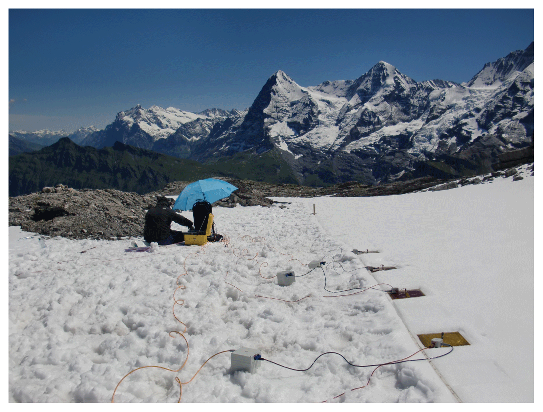
Figure 2Photograph of the measurements at profile B-SCH (Schilthorn area) in July 2016 with the Chameleon measurement device. The four plate electrodes are lying in line on the snow surface. The larger yellow box is the base unit which is connected by cables to the electrodes with the cubic grey remote units in between.

Download

The photograph in Fig. 2 shows an example of the equipment layout in the field. The plate electrodes, which are covered with Kapton foil for galvanic decoupling, were arranged in a profile line. They are connected by cables through a probe and a remote unit to the base unit (Przyklenk et al., 2016), which controls the measurements. The surface at the time of the measurements was covered by a layer of snow, which was frozen on the top. The depth of this snow layer was separately measured every 2 m using a dipstick for later validation of the results. Measurements were made along the profile in a dipole–dipole configuration (a=1 m) for several electrode spacings ($n=\mathrm{1}-\mathrm{6}$). They were not carried out with the same electrode spacing throughout the profile. Measurements with wider electrode spacing and corresponding larger penetration depth were carried out only on the first half of the profile.

2.2 Tromsø

The measurements in Norway were made in 2015 on the frozen Lake Prestvannet near the town of Tromsø. Figure 3 shows the geographical position of the area and the test site. In Fig. 3b, a part of the peninsula Tromsøya with the city Tromsø and the lake is visible. Lake Prestvannet covers an area of about 10 ha, has a maximum depth of 4 m and is covered by ice most of the year (Stabbel, 1985). Although no quantitative statement is made, investigations of the lake water qualitatively indicate a high salinity (https://memim.com/prestvannet.html, last access: 29 August 2019). The part of the lake where the test site is located is shown in panel (c), including the profile, which has an extension 33 m long and crosses the shore of the lake. The shore was covered with a layer of snow, the lake itself was frozen and measurements took place directly on the lake ice. Starting the profile on the lake and ending at the shore, the transition to the lake surface is at about profile coordinate 20.5 m.

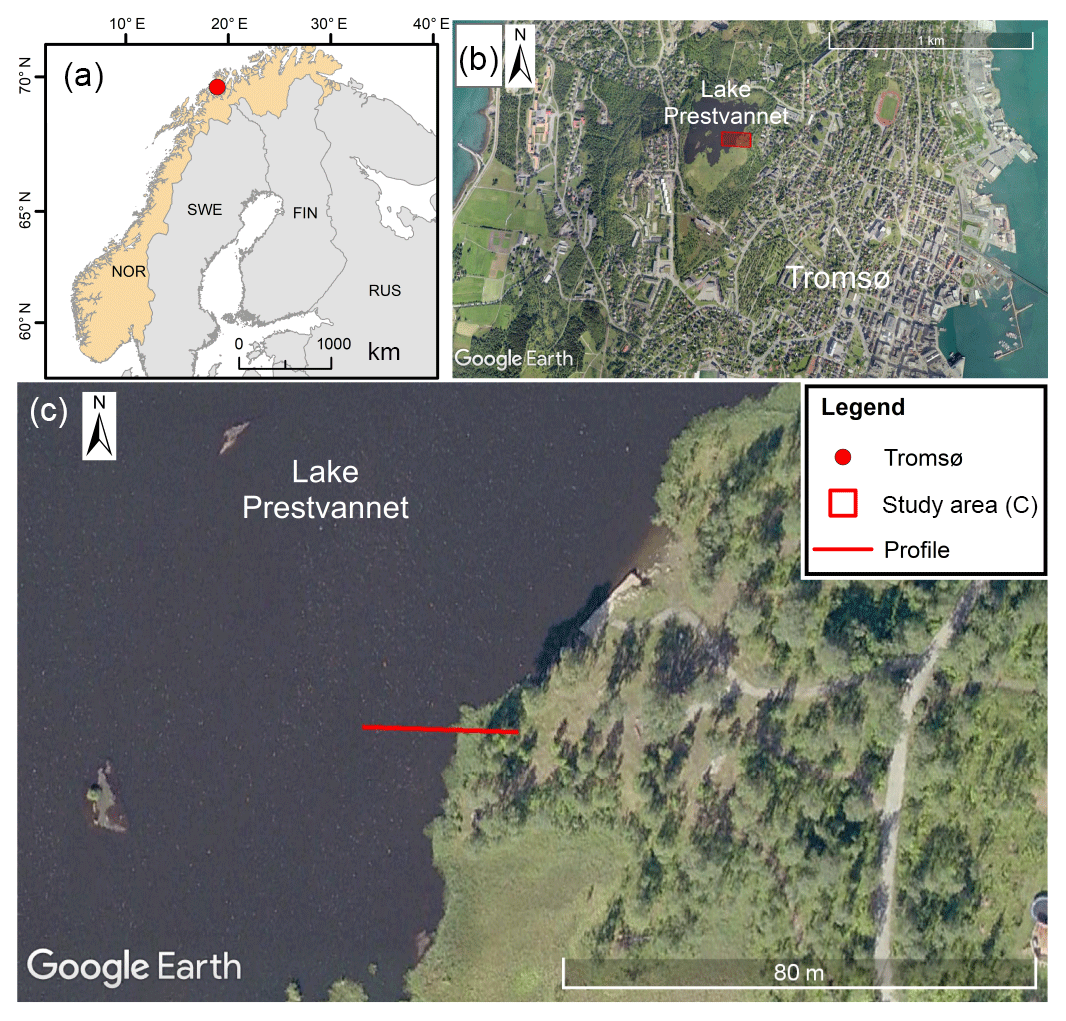
Figure 3Geographical maps of Lake Prestvannet. The location in the northern part of Norway is shown in part (a) by the red dot. The lake is located on the peninsula Tromsøya, presented in panel (b), close to the city Tromsø (© Google Earth). A detailed view of the test site is given in panel (c), showing the profile crossing the boundary from the lake to the shore (© Google Earth).

The measurements were taken with a fixed electrode spacing in Wenner configuration (a=1.5 m) to investigate differences in the measured data due to the sub-vertical lake–shore boundary. The penetration depth of the measurements therefore has a maximum of 1.5 m (Militzer and Weber, 1985). Additional measurements indicated that the boundary to the liquid water was at a minimum of 4 m depth, below the penetration depth of the data.

3.1 Cole–Cole model

The electrical permittivity and the resistivity are not constant values in most cases but vary with frequency. Polarizable materials, e.g. water-saturated sediments or mineralized rocks, exhibit a strong frequency dependence of electrical parameters (Zorin and Ageev, 2017). This is especially true in periglacial areas, for materials with pure ice or large ice contents (Petrenko and Whitworth, 2002; Bittelli et al., 2004; Stillman et al., 2010). Przyklenk et al. (2016) investigated several parametrizations of the frequency dependence of resistivity and permittivity. They suggest the use of the Cole–Cole model (CCM) (Cole and Cole, 1941), which provides reasonable results when fitting the spectral data of CCR measurements. For variable data with more spectral shape, a dual CCM, corresponding to a model of a two-component mixture, might be necessary for the evaluation of the impedance spectrum. For our studies, we decided to use the single CCM, which includes just one material, because it can fit our data with a minimum number of parameters. For the relative complex permittivity, the single Cole–Cole model is expressed by

The description of the frequency dependence of the electrical parameters is based on five Cole–Cole parameters: the DC resistivity ρ_DC, a low-frequency limit ε_DC, a high-frequency limit ε_HF, which is referred to in the literature as the dielectric constant, the relaxation time τ and the relaxation exponent c. The positive relaxation exponent can range up to a maximum value of 1, for which the model simplifies to the Debye model (Petrenko and Whitworth, 2002). The parameters are directly related to a physical context. Thus, they are material-specific parameters for which ranges of literature values are known and can be used for a discussion of the inversion results.

3.2 Operating range

There is a parameter range in which the CCR method is feasible in the sense that the underlying assumptions are fulfilled and the physical process that is used to determine the spectral behaviour of permittivity and conductivity actually dominates. The term “parameter range” refers to the frequency, spatial scale (i.e. distance between transmitter and receiver), and electrical conductivity and permittivity. The CCR method operates in the “geometric sounding” range, where the investigated volume and in particular the penetration depth depend only on the location and the distance between transmitter and receiver. This is the same condition that applies to the ERT method.

The two processes that need to be investigated because they may limit the operating range of CCR are electromagnetic induction (EMI) and wave propagation. Electromagnetic induction currents are caused by the time-varying magnetic fields which always co-exist with electric fields. Several methods are based on EMI, which is particularly important if the conductivity is large. Wave propagation is the basis of ground-penetrating radar (GPR) methods, and is particularly important for very large frequencies.

For an assessment of the relative importance of the processes, we use the consideration by Weidelt, 1997, who compares the wavelengths (or their inverse, the wavenumbers) of the three processes with each other. The wavelength of EMI is equal to the skin depth, given by

where μ is the magnetic permeability, where in this context it is sufficient to use the vacuum value, which is ${\mathit{\mu }}_{\mathrm{0}}=\mathrm{4}\mathit{\pi }\times {\mathrm{10}}^{-\mathrm{7}}\frac{Vs}{Am}$.

The wavelength of wave propagation is given by

For geometric sounding, the signal is composed of many different wavelengths, but for an estimate of the relative importance of the processes, it is feasible to use an appropriate measure of the spatial scale of the electrode configuration (i.e. the electrode distance a for Wenner configuration) as the dominant wavelength. The equation that allows us to compare the three processes is (Weidelt, 1997)

where γ is the complex wavenumber including all three processes, and the symbols G, EMI and WP stand for the geometrical sounding, electromagnetic induction and wave propagation term, respectively. The process corresponding to the largest term will dominate, and the other terms may be negligible, depending on their magnitude.

Since there are four parameters controlling Eqs. (6)–(8), which also depend on each other (i.e. permittivity depends on frequency), it is difficult to give an operating range of general validity. It seems more feasible to evaluate the terms in Eq. (8) for specific conditions. For the measurements discussed in this paper, we can carry out the following estimates. The maximum frequency of our system is 240 kHz. Assuming a minimum relative permittivity of 3, the minimum wavelength of wave propagation given by Eq. (7) is 722 m. The minimum wavelength of EMI given by Eq. (6) depends on electrical resistivity. Assuming ρ=100 Ωm as the minimum resistivity, which is a little smaller than the minimum values actually encountered, we obtain approximately 10 m for the minimum EMI wavelength. From Eq. (8), it is clear that the geometrical sounding term will be the minimum for the largest electrode spacing, and therefore we use our largest spacing a=1.5 m in Eq. (8) to obtain a worst-case estimate.

With these numbers for the wavelengths, we obtain for the magnitudes G=17.5, EMI =0.02 and WP $=\mathrm{7.6}\times {\mathrm{10}}^{-\mathrm{5}}$. Therefore, the wave propagation term is by far the smallest and can safely be neglected; the EMI term is still significantly smaller than the geometrical sounding term. We therefore assume that for the data discussed here, EMI is also negligible, in case of high resistive environments and small electrode distances (Fiandaca, 2018). Nevertheless, we are also aware that a comprehensive assessment requires precise modelling of the equations, which will be the subject of future work. If we chose a larger electrode spacing, a=30 m, then EMI =8, and this would be of the same order of magnitude as G, and we would have to carry out a more thorough analysis.

In addition to these purely physical considerations, we also have to take technical issues into account, such as coupling of the capacitive electrodes, and electromagnetic coupling between cables and the ground, which are less simple to estimate or to correct for. Therefore, we consider it necessary to gain experience and to test the entire system under a variety of conditions.

3.3 Single site inversion

The single site inversion was the primary method used in Przyklenk et al. (2016). In this spectral approach, the data of each measured four-point array are inverted separately, i.e. without influence of other measurements. Under the conditions of geometrical sounding, the penetration depth of the measurement is only controlled by the geometric size of the configuration, i.e. the geometry factor K, in contrast to the frequency sounding where the frequency-dependent skin depth describes the penetration depth (McNeill, 1980).

The fit of the measured spectral data of the magnitude $\left|Z\right(f\left)\right|$ and phase shift φ(f) is obtained under parametrization of the complex impedance (Eq. 2) by the single Cole–Cole equation (Eq. 5). The inversion is based on the model of a homogeneous half-space. From the result of the inversion, the five Cole–Cole model parameters can be extracted. Moreover, the single site inversion has the possibility to take the sensor height effects into account. By using the mean electrode height h as an additional free inversion parameter, it is possible to include the effect of electrode height and at the same time determine its value. Thereby, capacitively coupled measurements taken under conditions of strong height influence, in particular on low resistive subsurfaces, can also be evaluated. If the height is neglected during inversion, this can in principle lead to a distortion of the data and erroneous results. Since in the next step we use a conventional 2-D inversion code for spectral IP data, where the height effect is not included in the forward modelling, it is essential to test whether it is justified to neglect it. For this purpose, we carry out the single site inversion twice: first including the height effect by setting the height as a free parameter and once under the assumption of no sensor height, i.e. by fixing it to zero.

Figure 4 shows a representative example of the spectra for magnitude (a) and phase shift (b) from a measurement at profile B-SCH. The points indicate the measured data, and the lines are the calculated spectra for the best-fit model. Inversion is done with (CCM h_inv) and without (CCM h₀) determination of height. The calculated height for CCM h_inv is $\mathrm{7}\times {\mathrm{10}}^{-\mathrm{7}}\mathrm{m}$. This is so close to zero that the results exhibit no visible difference in the measured frequency range. The parameters of the Cole–Cole model, given in the caption of the figure, have no difference if rounded to a maximum of two decimal places.

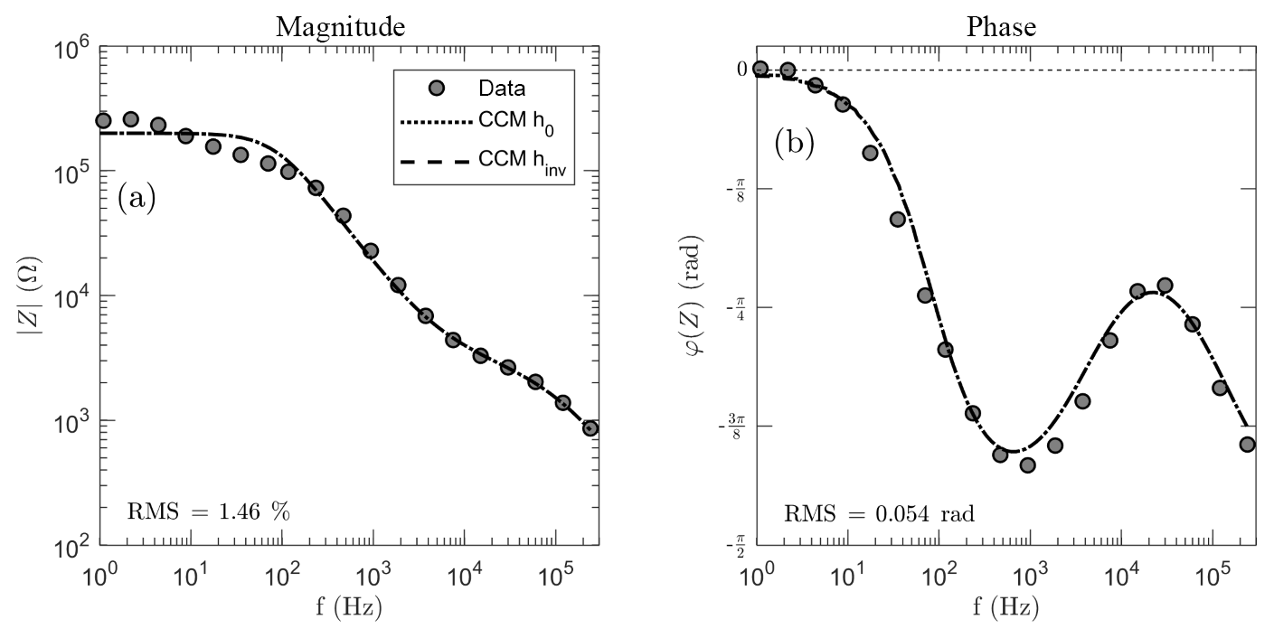
Figure 4Spectra for the magnitude (a) and the phase shift (b) of the impedance for measured data (dots) and inversion results by using the Cole–Cole model (CCM, lines). The inversion was carried out twice, with the assumption of zero electrode height (h₀) and by calculating the height as an additional inversion parameter (h_inv). The simulated curves of the two inversions can not be distinguished from each other. Data were measured at profile B-SCH, Schilthorn area, Switzerland, in a dipole-dipole configuration (a=1m, n=1). The CCM parameters are (h₀ and h_inv): ${\mathit{\rho }}_{\mathrm{DC}}=\mathrm{3.8}\times {\mathrm{10}}^{\mathrm{6}}\mathrm{\Omega }\mathrm{m}$, ε_DC=53, ε_HF=2.8, $\mathit{\tau }=\mathrm{3.6}\times {\mathrm{10}}^{-\mathrm{5}}\mathrm{s}$, c=0.82.

Download

The magnitude adopts a value of around 2×10⁵ Ω for low frequencies, where the curves converge to a constant value. The phase shift covers almost the entire range that is theoretically possible (0 to −90^∘). The values close to zero for low frequencies indicate a domination of conduction currents, whereas the deviation from zero for increasing frequencies indicates the increasing relevance of displacement currents. It is expected that for higher frequencies out of the measured range, the phase shift approaches the limit of −90^∘ where displacement currents dominate. The aim of measuring the intermediate range with the transition between both current mechanisms has been achieved in this case. The measured spectral signals in Fig. 4 are typical of the whole measurements on the profile. The values of magnitude are decreasing for larger configurations because of the increasing geometry factor. The phase shift shows the characteristic wavelike shape with a local minimum and maximum. The data fit of the single site inversion is reasonable, justifying the usage of the single Cole–Cole model.

In the case of Lake Prestvannet we assume a sub-vertical separation through the measurements over the lake shore. Two representative signals are shown in Fig. 5 to illustrate the difference between the characteristic curve shapes. The magnitude exhibits a stronger frequency dependence in the case of the land measurements and a higher value for low frequencies of about 1 order compared to the lake measurements. For the phase shift, the shape of the curve measured on the lake is flatter and the local minimum is at higher frequencies. The phase shift shows smaller dynamics for the lake than for the land measurements. The figure illustrates that the different ground materials provide significant differences in their response.

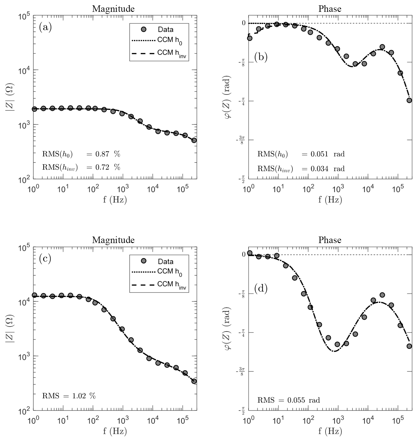
Figure 5Spectra of two measurements from the Tromsø site. Panels (a) and (b) show data from the lake and (c, d) data from a measurement on shore. The figure shows the measured data and the inversion results using the Cole–Cole model. The simulated curves with zero electrode height (h₀) and inverted height (h_inv) can not be distinguished, except for the phase shift of the lake measurement (b). Both measurements were taken in a Wenner configuration with a=1.5 m. The CCM parameters for the lake measurement are (h₀∕h_inv) ${\mathit{\rho }}_{\mathrm{DC}}=\mathrm{1.82}\times {\mathrm{10}}^{\mathrm{4}}/\mathrm{1.81}\times {\mathrm{10}}^{\mathrm{4}}\mathrm{\Omega }\mathrm{m}$, ${\mathit{\epsilon }}_{\mathrm{DC}}=\mathrm{374}/\mathrm{370}$, ${\mathit{\epsilon }}_{\mathrm{HF}}=\mathrm{8.80}/\mathrm{8.83}$, $\mathit{\tau }=\mathrm{4.2}\times {\mathrm{10}}^{-\mathrm{5}}/\mathrm{4.1}\times {\mathrm{10}}^{-\mathrm{5}}\mathrm{s}$ and $c=\mathrm{0.93}/\mathrm{0.93}$. The CCM parameters for the onshore measurement are (h₀ and h_inv) ${\mathit{\rho }}_{\mathrm{DC}}=\mathrm{1.2}\times {\mathrm{10}}^{\mathrm{5}}\mathrm{\Omega }\mathrm{m}$, ε_DC=670, ε_HF=12.8, $\mathit{\tau }=\mathrm{7.1}\times {\mathrm{10}}^{-\mathrm{5}}\mathrm{s}$ and c=0.84.

Download

The inversion was performed with and without the determination of sensor height. For the onshore measurement the estimated height is $\mathrm{2.5}\times {\mathrm{10}}^{-\mathrm{5}}\mathrm{m}$, which results in no visible difference between the simulated curves. For the lake measurement the fitted height of $\mathrm{1.2}\times {\mathrm{10}}^{-\mathrm{3}}\mathrm{m}$ leads to a visible difference for the phase shift (panel b). The two calculated spectra vary for the lowest frequencies. While the inversion with zero height (continuous line) converges towards zero, the version including height (dashed line) shows a deviation from zero consistent with the data. The data fit also shows a difference in terms of the root mean square (RMS), which is better for CCM h_inv. It is known from theory that the height dependence has stronger effects for lower frequencies and is stronger for the phase than for the magnitude of the impedance (Przyklenk et al., 2016). Our data, with a visible effect in the phase shift and negligible effect in the magnitude for the data set with the smaller impedance (panels a, b), are consistent with these theoretical results.

3.4 Influence of electrode height on Cole–Cole parameters

In the following, we analyse the dependence of the Cole–Cole parameters on the electrode height in some more detail. The reason why we perform this analysis is that the 2-D inversion used later is not able to consider non-zero electrode height. Therefore, the single site inversion was performed for every measured array of both field areas in both versions, with and without determining h. For every array, the five resulting Cole–Cole parameters were put into relation for both inversions, and the mean deviation in percent was calculated. This deviation is shown as a function of the estimated sensor height in Fig. 6.

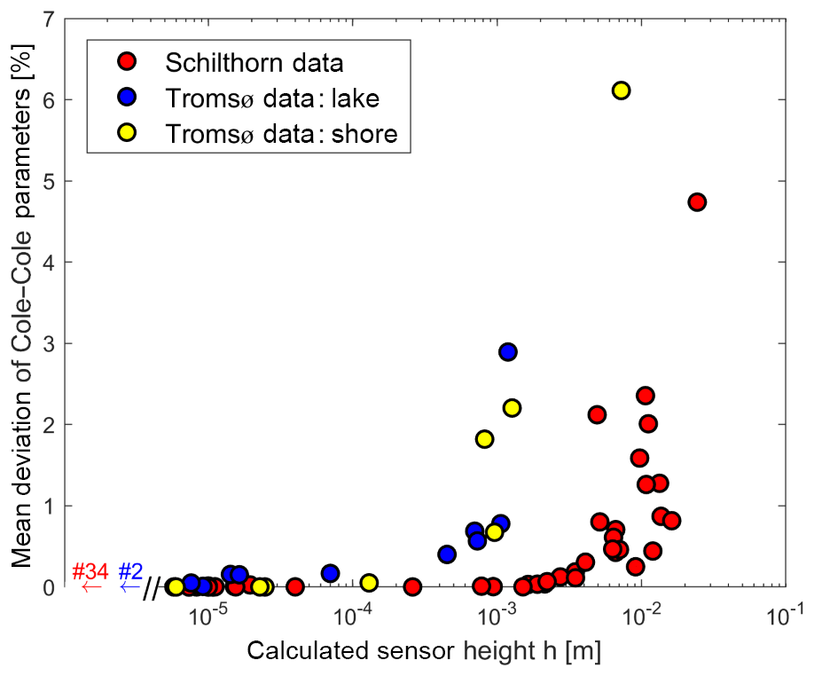
Figure 6Mean deviation of Cole–Cole parameters vs. sensor height. The deviation was calculated by performing the single site inversion with and without the determination of sensor height and calculating the ratio for all the five Cole–Cole parameters. The data are separately shown for all measurements at profile B-SCH (Schilthorn, red) and for Lake Prestvannet (Tromsø) on the lake (blue) and on shore (yellow). Values for sensor heights lower than $\mathrm{5}\times {\mathrm{10}}^{-\mathrm{6}}\mathrm{m}$ are not displayed but their number of measurements is shown.

Download

For larger sensor height, the Cole–Cole results are more affected. The Schilthorn data (red dots) show a strong increase in deviations from approximately $\mathrm{5}\times {\mathrm{10}}^{-\mathrm{3}}\mathrm{m}$ height on. For the Tromsø data, which are shown separately for the measurements on the lake (blue dots) and on the shore (yellow dots), this increase occurs for sensor heights about 1 order of magnitude lower. The different behaviour can be explained by the condition of lower electrical resistivities for the Tromsø measurements. As mentioned earlier, the height effect is stronger for lower ground parameters of resistivity and permittivity. Furthermore, for the Schilthorn data higher values of sensor height were determined. This could indicate that in case of the solid ice surface, as on the lake, the contact of electrodes to the ground is very smooth, resulting in a more homogeneous sensor height. On the other hand, the snow surface at Schilthorn builds a more porous ground. The loose material might cause a poorly defined contact and lead to an artificially increased apparent electrode height. The Schilthorn data show scattered sensor heights, which indicates the uncertainty in the electrode contact surface. It should be noted that the calculated sensor heights in Fig. 6 are shown only down to the lowest values of $\mathrm{5}\times {\mathrm{10}}^{-\mathrm{6}}\mathrm{m}$, but lower values were also determined. Investigations from Przyklenk et al. (2016) and Kuras et al. (2006) indicate that electrode heights lower than around 10⁻⁴ m do not effect the measured signal, especially under high resistive conditions. Smaller heights determined by the inversion are mainly due to numerical reasons and do not represent physical conditions. They can be seen as equal to zero. The determined values of the Schilthorn measurements range from less than 10⁻⁹ m up to centimetres. On the other hand the Tromsø results only vary from 10⁻⁷ m to the millimetre range.

Additional investigations, which will not be further elaborated here, have indicated that the parameters ρ, ε_DC and τ are generally more affected than ε_HF and c. That is consistent with the fact that the electrode height mainly affects the lower frequencies. All in all, the deviations of the Cole–Cole results are relatively small. Except for the two highest values in Fig. 6, their effect is smaller 3 %. These deviations are considered to be acceptable, compared to the typical Cole–Cole parameter resolution for inversions (Yuval and Oldenburg, 1997; Madsen et al., 2017). The results therefore justify the use of inversions without considering effective sensor height, as in the case of the 2-D inversion (see next section). It should be noted that under less favourable conditions, depending on the electrical parameters of the soil and the texture of the surface, neglecting the height can lead to larger errors. Neglecting height is therefore not a general recommendation, but has to be investigated separately for each application with different subsurface conditions. In the case of snow or icy ground, one additional benefit is that these are rather smooth surfaces, where the electrode height is small. On uneven surfaces, such as gravel and rock fields, an installation of the plate electrodes without height variations may be difficult to achieve.

4.1 Schilthorn

The measured data from profile B-SCH were evaluated with the 2-D inversion. The result is shown in Fig. 7, where several 2-D models for the five Cole–Cole parameters ρ, ε_DC, ε_HF, τ and c are shown colour-coded vs. the depth and horizontal coordinate. The dashed black line corresponds to the manually measured depth of the top snow layer.

Figure 7Result of the AarhusInv 2-D inversion for the data from the Schilthorn area along the profile B-SCH denoted in Fig. 1. The figure shows the sections of the five Cole–Cole parameters (a–e) defined by Eq. (5). The dashed line shows the separately measured depth of the snow layer, and the brighter parts represent the area where the depth of investigation is exceeded.

Download

In this context, it is important to discuss the resolution of the Cole–Cole parameters because it is known from previous studies that it can be difficult to reliably estimate relaxation time and frequency exponent (e.g. Madsen et al., 2017). Problems usually arise if the frequency where the phase peak occurs, which is related to the relaxation time, is outside the measured acquisition range. Weigand and Kemna (2016) discuss similar observations when average parameters are derived from spectral decomposition techniques. The particular benefit of our acquisition system is the wide frequency range compared to a conventional SIP system. As a result, all phase peaks corresponding to the relaxation times are in fact being measured. Therefore, we are confident that the Cole–Cole parameters of the inversion results are well determined. Nevertheless, we carried out additional experiments where we fixed the frequency exponent c, as suggested by Weigand and Kemna (2016). In that case, the data fit deteriorates, in the sense that the curve shape vs. frequency cannot be matched that well any more. We consider this as evidence that even c is not poorly constrained. The strong variability of c observed in the inversion results may be justified by the actual change in materials. Finally, we rely on the depth of investigation (DOI) as an objective measure in which region parameters are well constrained. The calculation of the DOI was described in Fiandaca et al. (2015). The brighter areas in Fig. 7 are those below the DOI, areas where the parameters can no longer be reliably estimated. This boundary differs for each parameter, having in most cases the deepest extent for the resistivity model. We are aware that other tools to assess parameter resolution may exist, but a comprehensive treatment of this subject is beyond the scope of this paper.

First, we focus on the structural aspects of the results. The structure is a little different for each of the five sections, but in general a structure of two layers can be recognized, representing the top snow layer and the underlying surface layer. Because of the additional snow depth measurements, the results of the inversion can be validated. Especially for ε_DC, the boundary of the snow layer agrees well with the corresponding parameter contrasts. Around profile metre 20, where the boundary indicates a ditch, it becomes particularly clear how precisely the layer structure is reflected by the low-frequency permittivity value (panel b). The layer boundary can also be seen from the result of the resistivity (panel a), where a highly resistive surface layer is followed by a more conductive material. Unlike in the ε_DC section, there is a continuous decrease in the value with the depth, which makes the layer transition appear more smoothly. The layer boundary is also apparent in the section of parameter τ (panel d). The relaxation exponent c (panel e) also indicates the boundary. In the lower layer, c is close to 1, corresponding to a Debye relaxation. Compared to the other parameters, less literature is available for the relaxation exponent and the values are close to each other. Therefore, c seems less suitable for an interpretation in terms of material properties. The high-frequency value ε_HF (panel c) is the only one which does not show a clear distribution. The range in this case is significantly smaller compared to the other parameters, which could make it more difficult to identify differences in materials based on ε_HF. This is the case in this example but could be different for other test sites or under different conditions. The region of slightly higher values at about 2 m depth on the second half of the profile could indicate a systematic change in the permittivity.

The two layers could be identified as the snow layer and the underlying bedrock, expected to be the limestone layer described by Rowan (1993), which could also be seen at some spots on the surface near the profile area. The resistivity and the relaxation time on the first half of the profile show some more variation underneath the snow. This could be caused by a third layer of weathered material on top of the bedrock or a possible ice cover underneath the snow, as described by Scherler et al. (2010).

The determined values in their dominating range for the two horizontal regions of profile B-SCH are compared to the literature in Table 1. The literature values of the different materials can vary over large ranges, which is mainly caused by the differences in physical conditions. For ice and snow the purity, density, salinity and temperature can strongly influence the electrical parameters (Auty and Cole, 1952; Arenson et al., 2015; Evans, 1965). New and soft snow, as was present in the case of the profile B-SCH, has a relatively low density, meaning an increase in resistivity towards more dense snow. For the literature values of ice the attribute “pure” means that there is no impurity caused by other materials in the ice/water, but there are still variations based on the physical conditions like temperature. If ground material is frozen, like on permafrost or seasonal frost, the measured signal is expected to react as a composition of the basic material and ice (Zorin and Ageev, 2017). The parameters for frozen ground are strongly dependent on the ice content and temperature (Arenson et al., 2015; Grimm et al., 2015). In the case of limestone, laboratory investigations of CCR by Murton et al. (2016) showed that the resistivity of a frozen limestone sample (10⁵ Ωm) can be 1 order of magnitude higher than for the same sample in an unfrozen state.

Table 1Results of the 2-D inversions on profile B-SCH and the profile on Lake Prestvannet and comparison with literature values for snow, ice, water and limestone, which is expected as bedrock material on B-SCH. The characteristic parameters from the inversions are given as the range for the two horizontal layers for profile B-SCH and the two vertical separated regions of lake and shore for the profile on Lake Prestvannet.

Literature values were taken from Arenson et al. (2015)¹, Evans (1965)², Achammer and Denoth (1994)³, Palacky (1988)⁴, Murton et al. (2016)⁵, Olatinsu et al. (2013)⁶, Seshadri et al. (2008)⁷, Artemov and Volkov (2014)⁸, and Auty and Cole (1952)⁹.

Download Print Version | Download XLSX

The electrical behaviour of water needs particular attention because the typical relaxation frequency of water is in the range of gigahertz (e.g. Artemov and Volkov, 2014). Consequently, the high frequency value ε_HF of about 5 will not be reached within our frequency range. Instead, the real dielectric permittivity exhibits a constant behaviour, denoted as the low-frequency value, which is commonly known as 80. However, a study by Seshadri et al. (2008) shows that even in water without solids another relaxation process takes place at lower frequencies in the range of hertz, associated with interfacial polarization due to ions. The dielectric permittivity therefore can reach values of more than 1000 at the lower boundary of our frequency range, especially if the water has a high electrolyte concentration.

In Table 1 (top row) the information of the inversion results (Fig. 7) is extracted and attributed to different layers. For the first layer, the estimated values agree for all Cole–Cole parameters with those of snow. For the area under the horizontal boundary, indicated by the clear change in parameters ρ_DC, ε_DC and τ, the estimated values are in agreement with the expected limestone layer. As the resistivity indicates a further separation, the area directly underneath the snow could either belong to an ice layer or be caused by a frozen state, followed by a less resistive part of the limestone. The observation that all other parameters except resistivity show no significant change in this area can be explained by the similarity of the parameters for ice and limestone, indicated by the literature values. The similarity and small range of high-frequency permittivity ε_HF of all corresponding literature values can explain the low variability and missing distinctness in this parameter section. In summary, the determined Cole–Cole parameters from the 2-D inversion are consistent with the literature values for the expected materials.

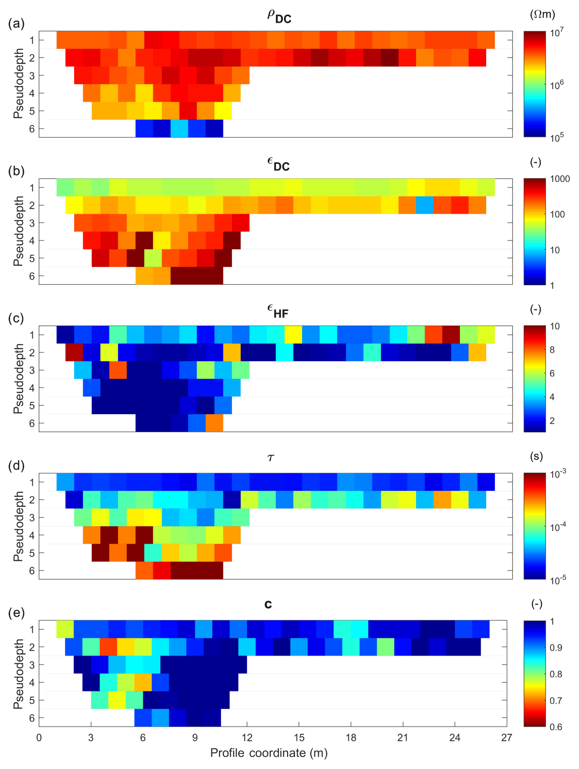
Figure 8Pseudo-sections of the five Cole–Cole parameters (a–e) calculated by the single site inversion for profile B-SCH. Measurements were performed for larger configurations on the left half of the profile.

Download

A comparison with the results of the single site inversion illustrates the differences of the inversion methods. Figure 8 shows the results for the same measurements as in Fig. 7 but evaluated by the single site inversion. The parameters are determined individually for each quadrupolar measurement. In order to represent the results in a two-dimensional structure, the parameters are assigned to a certain location according to the midpoint position and extent of the array. Thus, a two-dimensional pseudo-section is finally created for each parameter, which can provide a rough overview of the subsurface structure. The difference between Figs. 7 and 8 is that Fig. 8 represents an inversion result only with respect to frequency, but a pseudo-section with respect to the spatial distribution, whereas Fig. 7 is a full inversion result with respect to both frequency and space. As expected when comparing pseudo-sections with 2-D inversion results, overall structures are similar, but there are differences in detail. The low-frequency permittivity (panel b) and the relaxation time (panel d) systematically increase with depth, while the resistivity (panel a) shows a decrease with depth, all indicating a horizontally layered structure. As seen before in the 2-D results, the high permittivity value ε_HF exhibits a small range of values and does not show a systematic distribution, but fits in the range of the literature. Since the results of the deeper pseudo-layers always represent an integral value over the entire depth range, it has to be expected that clear boundaries between the layers can not be identified by this method. Therefore the measurements have to be analysed as functions of each other, as carried out by the 2-D inversion. However, since the inversion with respect to the frequency dependence is independent for the two methods, we take the qualitative consistency as evidence that our 2-D inversion is a feasible tool to invert spatial and frequency dependence at the same time.

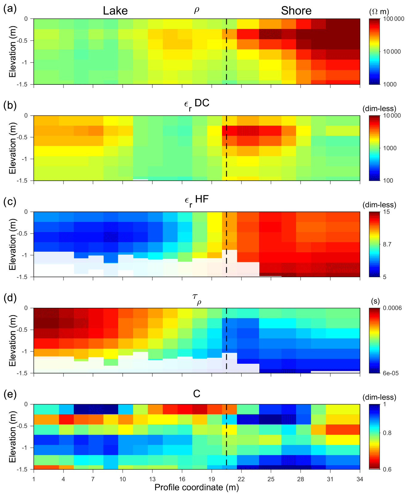
Figure 9Two-dimensional inversion result of the five Cole–Cole parameters (a–e) for the measurements at Lake Prestvannet denoted in Fig. 3. The surface boundary between lake and shore is at profile metre 20.5, indicated by the dashed line, where a change in most parameters can be recognized. The whitened areas are those where the value of DOI is exceeded.

Download

4.2 Tromsø

The investigations at Lake Prestvannet focus on the vertical transition from the lake to the shore rather than on the distribution with depth. In Fig. 9, the result of the AarhusInv 2-D inversion is shown for all Cole–Cole parameters. Measurements were carried out for just a small spacing (Wenner a=1.5 m), so the penetration depth is not more than approximately 1.5 m. Brighter areas are again below the DOI and the vertical black line indicates the surface position of the transition from the lake to the shore at profile metre 20.5. Except for the relaxation exponent c (panel e), in all models the transition is defined by a parameter change. The ranges of the estimated Cole–Cole parameters for lake and shore are given in Table 1 and can be compared to the literature values of snow, ice and water.

The high-frequency permittivity ε_HF (panel c) shows lower values for the lake than onshore. This parameter is somewhat specific because the variation from lake to shore is the only prominent variation, whereas the other parameters also show some structure within both sides. Compared to profile B-SCH (Fig. 7), where ε_HF has a small dynamic range with little spatial coherence, for the data of Lake Prestvannet both permittivity values ε_DC and ε_HF seem to be useful to distinguish different materials or the state of freezing. The low-frequency permittivity ε_DC (panel b) shows the transition from lake to shore, but exhibits additional variation on either side of the transition. The land side shows an anomaly close to the transition. The cause is not exactly known, but we hypothesize that it indicates a change in sediments. A detailed analysis, where the two properties of permittivity may be combined with resistivity in a multi-parameter analysis, may be a subject of future research. The relaxation time τ shows relatively homogeneous values for each of the sides. The fact that the relaxation times of snow are shorter than those of ice (Evans, 1965) is consistent with our results. The resistivity ρ_DC decreases from higher values on the snow-covered land side by about 1 order of magnitude on the lake. The relaxation exponent c shows small variations and poor spatial coherence, and is difficult to interpret in terms of material variations.

Onshore, the measurements were taken on the snow and the known values of snow are consistent for some parameters. Higher density of the snow could explain the much lower resistivity than obtained for the snow at B-SCH. However, in combination with the values of ε_DC, which are higher than expected for snow, this could indicate that the measurements are under the influence of the ground material beneath. For the frozen lake, the values estimated from the inversion are a bit higher than typical literature values for ice. However, it is known that the electrical parameters of frozen water bodies can be very different from those of pure ice. The lake ice could be a composition of ice and partly water, instead of a pure ice body. Such mixtures can result in higher values of permittivity. The high salinity of the lake can further increase the low-frequency permittivity of the water to the range of >1000 (Seshadri et al., 2008). This is significantly larger than the value of pure water of about 80 (Evans, 1965), and could explain the high ε_DC values determined by the inversion. At the high-frequency end in our frequency range, the value of ε_HF is probably also controlled by water (around 80 in that frequency range), which explains why our estimated value is larger than that expected for pure ice. Lower values of resistivity could also be explained by this composition because water has a lower intrinsic resistivity than ice. A similar observation was made by Przyklenk et al. (2016) during their discussion of measurements on mountain ice.

4.3 Data fit

For the assessment of the inversion results, we consider their quality in terms of the data fit. Because of being a spectral inversion, the inversion includes the fit of all measured data over frequency, corresponding to a spectral pair of magnitude and phase shift for every four-point array. In the following, the data misfit is expressed in terms of the weighted mean square error, where each difference is weighted by the inverse of the data error. This value is denoted by the symbol χ, and is a well-established measure of the misfit. Together with an additive regularization term, it is minimized during the inversion (Fiandaca et al., 2013).

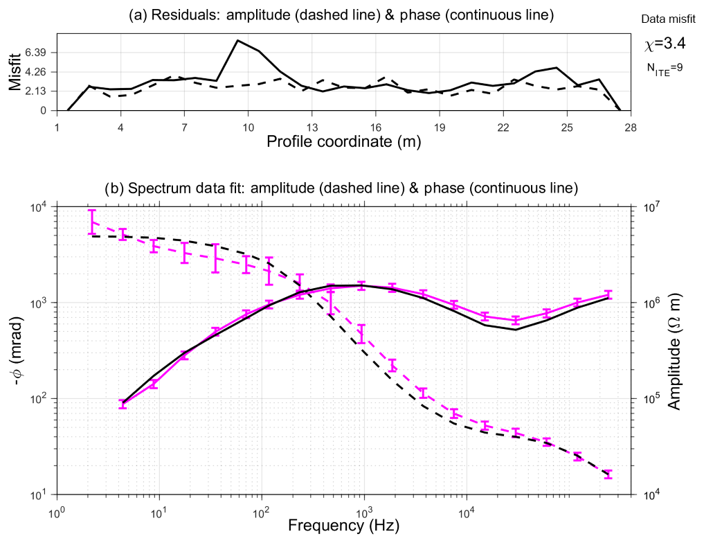
Figure 10Data fit of the 2-D inversion of profile B-SCH. Panel (a) shows the misfit of amplitude (dashed line) and phase shift (solid line) over the profile. Panel (b) shows an example of measured (red) and inverted (black) spectra of amplitude (dashed lines) and phase (continuous lines), which belong to the dipole–dipole measurement starting from profile metre 16 (a=1 m, n=1) along the profile direction (see Fig. 7). The measured data are the same as in Fig. 4, with resistivity instead of impedance, and phase shift on a logarithmic scale. The total data misfit is χ=3.4 after nine iterations. For each profile coordinate, the misfit of all data corresponding to this point was averaged to obtain the top panel (a).

Download

Figure 10 shows the data fit for the 2-D inversion of the Schilthorn measurements. The top panel (a) shows the misfit of amplitude and phase shift over the profile length. The residuals are averaged over all measurements with all configurations with the same midpoint. The total inversion misfit is χ=3.4, based on the average relative standard deviation of amplitude (0.16) and phase measurements (0.10). The inversion converged after nine iterations. The misfits of amplitude and phase are homogeneous over the profile, except around profile metre 10, where the phase misfit is significantly higher. As can be seen from Fig. 7, this is the area where ρ and τ show another change for the deeper region. The higher misfit corresponds to the data of larger configurations (dipole–dipole with $n=\mathrm{5},\mathrm{6}$), where the measured signals show slightly different curves than for the shallower measurements. The large misfit indicates that the deep structure should be treated with caution because it could be caused by difficulties in matching data.

Panel (b) of Fig. 10 shows the data fit of the spectrum, which was previously shown during the discussion of the single site inversion (Fig. 4). Data and inversion results are shown for the amplitude (dashed lines) and the phase (continuous lines). The amplitude is not exactly the same as the magnitude in Fig. 4, but was converted to the frequency-dependent resistivity (using Eq. 3). The negative phase shift is displayed on a logarithmic scale in milliradians. Some data points, in this case for the two lowest frequencies, that caused difficulties for the inversion code and were identified as outliers, are not shown. Overall, for both amplitude and phase shift, the shape of the spectrum is well matched. For several data points, the calculated curve is not within the data errors, which is reflected in a misfit value χ>1. The data errors are calculated by the device by stacking multiple measurements. Considering that broadband electrical data of 79 spectra were matched with a single 2-D model, we find the fit satisfactory. The 19 discrete measured frequencies seem to be sufficient to define the dispersion of permittivity.

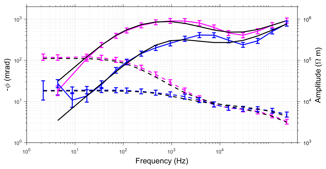
Figure 11Data fit of the 2-D inversion for two stations of the Lake Prestvannet profile. The blue lines correspond to a measurement at 11.5 m, which is on the lake, the red lines to an onshore measurement at 28 m, with the corresponding inverted spectra (black). Both were measured with a Wenner configuration (a=1.5 m). The measured data are the same as in Fig. 5. The amplitude is indicated by the dashed lines and the phase shift by the solid lines.

Download

Another example of data spectra is shown in Fig. 11 for the measurements taken at Lake Prestvannet. The data are the same as discussed in Fig. 5, with one lake measurement (blue) and one onshore measurement (red) corresponding to profile coordinates 11.5 and 28 m from Fig. 9. The total data misfit of the inversion is χ=1.8. The onshore spectra show some similarity to the Schilthorn spectra (Fig. 10). The amplitude and the phase shift are both matched very well. As mentioned before for the single site inversion, the spectra of lake and land show a different frequency-dependent behaviour. A slight difference between the measured and calculated data is visible for the phase of the lake measurement in the intermediate frequency range. This could indicate limitations of the single Cole–Cole model.

The sensor height effect is not negligible in this case. The lowest two frequencies seem to be affected and can not be matched by the inversion. This is the same effect as discussed previously during the single site inversion.