the Creative Commons Attribution 4.0 License.
the Creative Commons Attribution 4.0 License.
 | 30 Sep 2019
Changes of the tropical glaciers throughout Peru between 2000 and 2016 – mass balance and area fluctuations
Philipp Malz
Christian Sommer
Stefan Lippl
Alejo Cochachin
Matthias Braun
Glaciers in tropical regions are very sensitive to climatic variations and thus strongly affected by climate change. The majority of the tropical glaciers worldwide are located in the Peruvian Andes, which have shown significant ice loss in the last century. Here, we present the first multi-temporal, region-wide survey of geodetic mass balances and glacier area fluctuations throughout Peru covering the period 2000–2016. Glacier extents are derived from Landsat imagery by performing automatic glacier delineation based on a combination of the NDSI and band ratio method and final manual inspection and correction. The mapping of debris-covered glacier extents is supported by synthetic aperture radar (SAR) coherence information. A total glacier area loss of km2 (−29 %, −34.3 km2 a−1) is obtained for the study period. Using interferometric satellite SAR acquisitions, bi-temporal geodetic mass balances are derived. An average specific mass balance of kg m−2 a−1 is found throughout Peru for the period 2000–2016. However, there are strong regional and temporal differences in the mass budgets ranging from 45±97 to kg m−2 a−1. The ice loss increased towards the end of the observation period. Between 2013 and 2016, a retreat of the glacierized area of km2 (−16 %, −101.9 km2 a−1) is mapped and the average mass budget amounts to kg m−2 a−1. The glacier changes revealed can be attributed to changes in the climatic settings in the study region, derived from ERA-Interim reanalysis data and the Oceanic Nino Index. The intense El Niño activities in 2015/16 are most likely the trigger for the increased change rates in the time interval 2013–2016. Our observations provide fundamental information on the current dramatic glacier changes for local authorities and for the calibration and validation of glacier change projections.
- Article
(12830 KB) -
Supplement
(6063 KB) - BibTeX
- EndNote


Tropical glaciers in the Peruvian Andes are very sensitive to climate change and rapidly respond to varying climate settings (e.g. Kaser and Osmaston, 2002; Rabatel et al., 2013). A marked decrease in glacier coverage in Peru has been reported by various studies (e.g. Georges, 2004; Hanshaw and Bookhagen, 2014; Vuille et al., 2008) for the last decades. The recession of the Peruvian glaciers is proposed to have a significant impact on the downstream ecosystem and communities (Vuille et al., 2018). Glaciers act as an important temporal water reservoir for precipitation during the wet season. Glacier meltwater runoff buffers the water shortage caused by the low precipitation during the dry season (Kaser et al., 2003; Schauwecker et al., 2017). The shrinkage of glaciers leads to higher meltwater discharge and thus increases water supply to streamflow. However, glacier runoff decreases after the glacier loss reaches a critical transition point (Pouyaud et al., 2005). It has been suggested that some watersheds in the Cordillera Blanca have already crossed this critical transition point (Baraer et al., 2012). An unsteady or unreliable water runoff is known to cause several socio-economic issues (Drenkhan et al., 2019). Hydropower production and mining rely on a continuous water supply. Moreover, glacier runoff is an important water resource for irrigation and has the potential to affect large-scale but also subsistence agriculture (Vuille et al., 2018). It also impacts the Andean ecosystems. For example, the bofedales (high-altitude wetlands in the Andes) are very sensitive to changes in glacier runoff and a depletion of the meltwater is likely to cause them to shrink (Polk et al., 2017). Additionally, the glacier retreat leads to the formation and extension of pro-glacial lakes (Hanshaw and Bookhagen, 2014; Lopez et al., 2010) threatening downstream areas due to their potential to cause glacier lake outburst floods (GLOFs). In the Cordillera Blanca, several GLOFs have harmed local communities in the past. The most dramatic was the disaster in 1941 when large parts of the city of Huaraz were destroyed by a GLOF event, leading to ∼1800 casualties (Carey, 2010). However, the possibility of GLOFs is present throughout the tropical Andes (Cook et al., 2016; Hoffmann, 2012).
Several studies have been carried out to map and quantify changes in the glacier area in Peru. The majority of the analyses have focused on Peru's largest glacierized region, the Cordillera Blanca (e.g. Baraer et al., 2012; Georges, 2004; Hastenrath and Ames, 1995; Racoviteanu et al., 2008; Silverio and Jaquet, 2005, 2017; Unidad de Glaciologia y Recursos Hidricos, UGRH, 2010), and revealed significant glacier retreat in the last decades. The most recent studies reported a glacier recession in the Cordillera Blanca of −46 % between 1930 and 2016 (Silverio and Jaquet, 2017) and −33.5 % between 1975 and 2016 (Veettil, 2018). In other glacierized regions in Peru, distinct glacier retreat was observed as well. In the second largest glacierized mountain range in Peru, the Cordillera Vilcanota, an area loss of −32 % in the period 1985–2006 (Salzmann et al., 2013) and −30 % in the period 1988–2010 (Hanshaw and Bookhagen, 2014) was revealed. The only countrywide estimation of glacier area changes was carried out by the UGRH (2014). They estimated a total glacier retreat of −42.64 % from the first Peruvian glacier inventory of 1970 (Hidrandina SA, 1989) and the recent inventory covering the period 2003–2010 (UGRH, 2014). So far, no multi-temporal nor recent quantification of glacier area changes throughout Peru is available, only studies at regional levels.
There are a few studies dealing with surface elevation and ice volume–mass changes in Peru. Changes in the ice volume of m3 have been derived from aerial photographs and GPS point measurement data for three glaciers in the Cordillera Blanca by Mark and Seltzer (2005) for the period 1962–1999. Huh et al. (2017) calculated the surface elevation changes of six glaciers in the Cordillera Blanca by means of photogrammetric digital elevation models (DEMs) and lidar measurements. They found glacier-wide average surface lowering ranging between −9.5 and −64.06 m in the period 1962–2008. In the Cordillera Vilcanota, Salzmann et al. (2013) estimated volume changes of −40 % to −45 % based on inventory parameters for the period 1962–2006. Large-scale mass balance estimates covering Peru are the following: a mass balance estimation for the “low latitudes” of kg m−2 a−1 based on the upscaling of glaciological mass balance measurements covering the period 2003–2009 (Gardner et al., 2013), modelled surface mass balance of kg m−2 a−1 for the Andes north of 27∘ S in the period 1979–2014 (Mernild et al., 2017), an upscaled mass balance of Gt a−1 ( kg m2 a−1) for the same region using glaciological and geodetic mass balances between 2006 and 2016 (Zemp et al., 2019), a mass balance calculation throughout South America (excluding Patagonia) of Gt a−1 using space-borne gravimetric measurements from the Gravity Recovery and Climate Experiment (GRACE) for the period 2000–2010 (Jacob et al., 2012), and a geodetic mass budget of Gt a−1 ( kg m−2 a−1, ice density scenario: 850 kg m−3) derived from interferometric SAR (InSAR) measurements for the period 2000–2012/13 including glaciers in Bolivia (Braun et al., 2019). The first three cover large areas and thus the mass balance signals of glaciers in Peru or even smaller regions cannot be derived. The latter uses the glacier boundaries defined by the Randolph Glacier Inventory (RGI) 6.0. The RGI 6.0 has certain limitations in this region (RGI Consortium, 2017), which can lead to biases in the mass balance computation (Sect. 6.2).
Up to now, a spatially detailed and multi-temporal quantification of glacier changes throughout Peru is missing. In order to address this issue, this work aims to continue and expand the glacier monitoring of previous studies by carrying out a comprehensive analysis of glacier area changes and mass balances throughout the Peruvian cordilleras for the observation period 2000–2016 based on multi-sensor remote sensing data. The main objectives of this study are
-
to obtain a temporally and methodically consistent evaluation of countrywide glacier area changes
-
to assess geodetic glacier mass balances and their temporal variations throughout Peru
-
to identify relations between glacier fluctuations, changes of climatic variables, and topographic parameters.
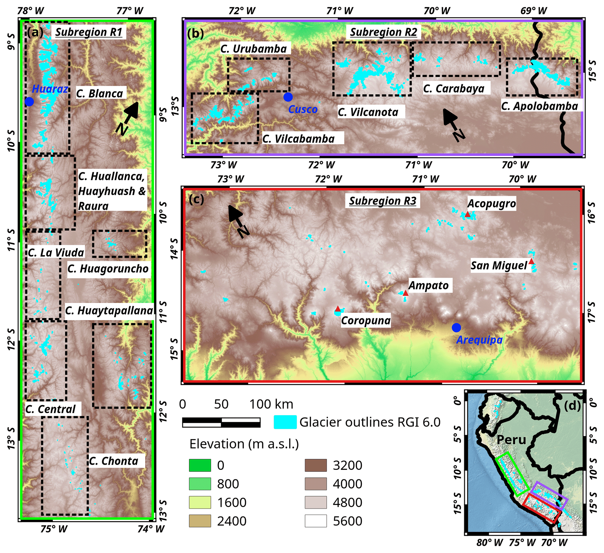
Figure 1General maps of study region. Panels (a–c): glacier subregions in Peru according to Sagredo and Lowell (2012); (a) subregion R1: northern wet outer tropics; (b) subregion R2: southern wet outer tropics; (c) subregion R3: dry outer tropics. Panel (d): overview map of Peru. Coloured rectangles indicate the locations of the subregions (same frame colours). Light blue areas: glacier coverage based on RGI 6.0. Background: SRTM DEM © NASA.
Peru is home to the majority of tropical glaciers worldwide. About 70 % of all tropical glaciers, covering an area of 1602.96 km2 (RGI 6.0), are located there. The Peruvian Andes are subdivided into three major mountain ranges, the Cordilleras Occidental, Central, and Oriental, from west to east, and several smaller cordilleras (Fig. 1). According to Sagredo and Lowell (2012), the glacierized areas are divided into three subregions based on their climatic settings.
-
R1 is the northern wet outer tropics, with a high mean annual humidity of 71 %, nearly no seasonality of the temperature (annual mean: 1.6 ∘C; variability of mean monthly temperature ∼1 ∘C), and a total annual precipitation of 815 mm. R1 ranges from the Cordillera Blanca southwards to the Cordillera Chonta and also includes the Cordilleras Huagoruncho and Huaytapallana further east.
-
R2 is the southern wet outer tropics, with moderate mean annual humidity of 59 %, an annual variability of the mean monthly temperature of about 4 ∘C (annual mean: 1.6 ∘C), and a total annual precipitation of 723 mm. R2 ranges from the Cordillera Vilabamba westwards to the Cordillera Apolobamba (partly located in Bolivia, but included completely in this study).
-
R3 is the dry outer tropics, with low mean annual humidity of 50 %, a mean annual temperature of −4.0 ∘C (variability of the mean monthly temperature of ∼5 ∘C), and low total annual precipitation of 287 mm. R3 ranges from the Cordillera Ampato westward to the Cordillera Volcánica.
The annual variability of precipitation shows a strong seasonality in all three subregions (Sagredo and Lowell, 2012) with a dry season during austral winter from May to September and a wet season during austral summer from October to April. The glaciers accumulate mass almost exclusively during the wet season, whereas the lower reaches of the glaciers experience ablation throughout the year (Kaser, 2001). Thus, slight variations in precipitation and temperature can lead to strong changes of the glacier mass balances (Francou Bernard et al., 2003), but also surface albedo and radiation significantly affect the mass budget of tropical glaciers (Favier et al., 2004; Wagnon et al., 1999). Moreover, the reaction of the glaciers in the tropical Andes to changing environmental conditions is nearly immediate (Vuille et al., 2008). The El Niño–Southern Oscillation (ENSO) has a strong impact on climate and thus the glacier mass balances in Peru (Garreaud et al., 2009; Maussion et al., 2015). El Niño events typically lead to pronounced glacier mass losses due to an induced precipitation deficit and above-average temperatures, whereas during La Niña periods the opposite conditions lead to reduced mass losses or even mass gain (Favier et al., 2004; Vuille et al., 2008).
Glaciological mass balance measurements are carried out at several glaciers in the study region by the UGRH, a subdivision of the Autoridad Nacional del Aqua (National Water Administration). However, observations are available in the World Glacier Monitoring Service (WGMS) database only for two glaciers covering our study period 2000–2016. Continuous annual mass balance observations have been documented at Artesonraju Glacier and Yanamarey Glacier since 2004. At some additional glaciers, mass balance programmes were initiated later and the data are not yet archived in the WGMS database.
Space-borne remote sensing data from different sensor systems are collected to perform this comprehensive study on glacier changes in the period 2000–2016. Synthetic aperture radar (SAR) data are used to obtain information on glacier surface elevation changes and mass balances. Digital elevation models (DEM) derived from interferometric SAR acquisitions at different time steps are used to compute surface elevation change information. As the elevation reference at the start of our observation interval, the void-fill LP DAAC NASA version 3 SRTM DEM (NASA JPL, 2013) is used. It is based on bistatic C-band SAR data, acquired during the Shuttle Radar Topography Mission (SRTM) by the National Aeronautics and Space Administration (NASA) and the German Aerospace Center (DLR) in February 2000. DEMs of later dates are generated from bistatic X-band SAR imagery of DLR's TanDEM-X (TDX) mission, which started in 2010 (Zink et al., 2011) (Sect. 4.2). Both SAR missions acquired data using different radar bands. Signal penetration of different radar frequencies in glacier surfaces depends on water content and the density of upper layers. This can lead to biases when comparing elevations on glacierized areas. Thus, we tried to select only imagery from the same season as the SRTM data in order to obtain acquisitions with similar glacier surface conditions and to avoid seasonal mass balance biases. In early 2013, an almost complete coverage of the glacierized regions in Peru could be obtained (early 2012 at subregion R1 as well as for comparison with Braun et al., 2019). Only a small fraction of the glacierized areas in subregion R3 had no coverage by TDX in early 2013. TDX imagery from early 2014 is used to fill the gaps (Sect. 5.2). A second temporally consistent coverage of the Peruvian glaciers by TDX data is available for 2016, though acquired primarily in the months of October and November, which mark the end of the dry season and beginning of the wet season. Typically, negligible accumulation occurs during the dry season and ablation dominates the glacier mass budget (Favier et al., 2004; Kaser, 2001; Veettil et al., 2017b). Thus, the mass balances for observation periods ending in 2016 are slightly biased towards more negative values due to this seasonal offset in the data. It is difficult to adequately quantify this temporal bias. Therefore, no correction is employed in the analysis and our computed mass loss rates represent upper bound estimations for the periods 2000–2016 and 2013–2016. A summary of the 331 analysed TDX scenes is provided in Supplement Table S1 and the spatial coverage of the subregions is plotted in Fig. S1 in the Supplement.
The RGI 6.0 Region 16 “Low Latitudes” covers all glacierized regions in Peru. The outline dates range between 2000 and 2009 in Peru. Thus, it does not represent the glacier extent at a specific moment. Moreover, it is mentioned in the RGI 6.0 Technical Report (RGI Consortium, 2017) that significant snow contamination caused difficulties in the glacier delineations, especially in southern Peru, and that a more rigorous demarcation could decrease the total glacier area. The Peruvian glacier inventory compiled by UGRH (2014) is also not temporally consistent. It covers the period 2003–2010. In order to use temporally appropriate glacier outlines for the mass balance evaluations and to map coincidental glacier area changes, we decided to generate a consistent database of countrywide glacier extents that correlates with the dates of our coverages of interferometric SAR data (see above). Cloud-free multispectral images from Landsat 5 TM and Landsat 8 OLI are required from the United States Geological Survey (USGS). Imagery, preferably during the dry season, is selected to reduce distortions due to temporal snow cover. For all subregions, a complete coverage in 2000 and 2016 is available. In subregions R1 and R2, cloud and snow cover forced us to map a small fraction of the glacierized regions using imagery from 2014 (Sect. 5.1). An overview of the analysed Landsat imagery is presented in Table S2. The Cordillera Blanca is the only mountain range with a considerable debris-covered glacier fraction. Therefore, the mapping of the glacier extents in this area is supported by interferometric analysis of repeat pass SAR acquisitions from the TerraSAR-X and Sentinel-1 satellite missions.
ERA-Interim reanalysis data (Dee et al., 2011) covering the period 1979–2017 provided by the Center for Medium-Range Weather Forecasts (ECMWF) are used to evaluate climatic changes and to identify correlations between glacier fluctuations, skin temperature, total precipitation, and downward surface thermal radiation. Monthly Oceanic Nino Index (ONI) data are applied as a proxy for ENSO events, which is available from the National Oceanic and Atmospheric Administration (NOAA) Climate Prediction Center (http://origin.cpc.ncep.noaa.gov/products/analysis_monitoring/ensostuff/ONI_v5.php, NOAA Climate Prediction Center, 2018). According to NOAA's definition, ONI values above +0.5 indicate El Niño events, whereas La Niña is present when ONI values are below −0.5.
4.1 Glacier inventory
Since the manual delineation of glacier extents is laborious, time-consuming, and subjective, several methods have been developed to automatically map glacier outlines based on multispectral images (Veettil and Kamp, 2017). The most widely used and robust approaches are the computation of the normalized difference snow index (NDSI) or the band ratio (BR) and the application of a threshold value to differentiate between on- and off-glacier areas (GLIMS algorithm working group, 2004; Paul et al., 2013). In this study, we first used the NDSI to classify glacier areas and combined it with BR information to improve the mapping in areas affected by shadows. NDSI maps generated from top-of-atmosphere reflectance values show a better performance than NDSI maps based on digital number values. For the BR computation, digital number values are taken. The threshold value selection is supported by high-resolution satellite imagery (Google Earth) from the respective dates. A NDSI threshold value of 0.8 is selected, which is higher than the thresholds of 0.5–0.6 applied by other studies in this region (e.g. Silverio and Jaquet, 2005; Veettil et al., 2017). This offset might be induced by the application of top-of-atmosphere reflectance values instead of digital number values. The threshold for the BR data is set to 1.7 for Landsat 5 TM and 1.5 for Landsat 8 OLI data. Finally, polygons of the glacier outlines are generated from the computed glacier masks.
The detection of the debris-covered glacier termini extents in the Cordillera Blanca is difficult using multi-spectral imagery. Therefore, we generated SAR coherence maps from repeat-pass SAR acquisitions to distinguish the debris-covered ice from the surrounding ice-free areas (Atwood et al., 2010; Lippl et al., 2018). The surface structure of the debris-covered glacier areas changes over time due to the dynamics and melting of the underlying ice. This leads to a temporal decorrelation of the backscattered SAR signal of repeat-pass SAR imagery and thus to lower coherence compared to the surrounding ice-free areas. This difference in coherence facilitates the delineation of the debris-covered ice areas. Data from the Sentinel-1 mission are used to map the debris-covered areas in 2016. No suitable repeat-pass SAR acquisitions are available for the Cordillera Blanca in 2013. Thus, we had to rely on TerraSAR-X and Sentinel-1 data from 2014 to map the outlines of the debris-covered glacier tongues. In 2000 (and ±1 year), only repeat-pass SAR data are available from the European Remote Sensing (ERS) satellite with a repetition cycle of 1 d. Due to this short temporal baseline, a separation between debris-covered ice and surrounding ice-free areas is unfeasible. Consequently, we combined our outlines from 2000 with the manually delineated debris-cover masks available from the Global Land Ice Measurements from Space (GLIMS) database from 2003 based on SPOT imagery (Racoviteanu, 2005).
The catchment discriminations of the RGI are applied to split the resulting polygons into individual glacier basins. In the next step, the glacier inventories are visually inspected and misclassified areas are manually corrected. These manual corrections are supported by high-resolution imagery from the respective years (Google Earth). According to the RGI 6.0 Technical Report (RGI Consortium, 2017), topographic parameters (minimum, maximum and median elevation, mean slope, and aspect) of the individual glacier basins are computed using the void-filled SRTM DEM as an elevation reference. Finally, the areas (S) of the complete inventories and of each glacier are measured in UTM projection (UTM Zone 18S for subregion R1 and UTM Zone 19S for subregion R2 and R3). The uncertainties of the area gauging (δS) are calculated following the approach of Malz et al. (2018) based on an error evaluation of 3 % for alpine glacier outlines derived from Landsat images (Paul et al., 2013). This estimate is scaled by the area-to-perimeter ratio of the studied subregion compared to the area-to-perimeter ratio of Paul et al. (2013) in order to account for differences in the shape of the glacierized areas.
4.2 Elevation change
Surface elevation change information is computed by differencing DEMs from SRTM and TDX data. DEMs are derived from the bistatic TDX imagery following the differential interferometric approach (e.g. Malz et al., 2018; Seehaus et al., 2015; Vijay and Braun, 2016), which is briefly summarized in the following.
First, acquisitions from the same relative orbit and date are concatenated in the along-track direction. A differential interferogram is computed using the void-filled SRTM DEM as elevation reference. In the next steps, the interferogram is filtered and unwrapped by applying the branch cut and minimum cost flow algorithm, and the unwrapped differential phase is transferred into differential elevations. Subsequently, the topographic information of the SRTM DEM is added to obtain absolute height information and finally the product is geocoded and orthorectified. The DEMs are visually checked for phase jumps and the best results of both phase-unwrapping methods are selected for further processing. Areas affected by remaining phase jumps are masked out.
The TDX DEMs need to be precisely horizontally and vertically coregistered to the respective reference DEM (SRTM for 2000, TDX for 2013) in order to accurately map elevation changes on the glacierized areas. Figure S2 illustrates the applied processing chain used to perform this coregistration. First, smooth stable reference areas are defined by masking out vegetation, water, and glacier areas. The vegetation and water masks are derived from region-wide cloud-free Landsat 8 mosaics and using a normalized difference vegetation index (NDVI) threshold of 0.3 and a normalized difference water index (NDWI) threshold of 0.1. Additionally, a slope threshold of 15∘ (of the respective reference DEM) is applied. Thereafter, the TDX DEMs are bilinearly vertically corrected for offsets to the reference DEM, which are measured for the defined stable regions. Subsequently, a horizontal coregistration between the reference DEM and the TDX DEMs is carried out following the widely used approach of Nuth and Kääb (2011). Afterwards, a second bilinear vertical coregistration of the TDX DEMs to the reference DEM is run to reduce any biases that remain. Finally, the coregistered TDX DEMs are merged to a regional DEM mosaic, which include a date stamp for each grid cell.
To obtain elevation change rates Δh∕Δt of the respective study periods, the SRTM DEM and the TDX DEM mosaics are differentiated. The mean date of the 11 d SRTM mission (16 February 2000) is assigned to the SRTM DEM. Since data voids in the SRTM DEM are filled with data from other sources (no date information available), the non-SRTM data values are masked out using the coverage information provided by LP DAAC NASA. Numerous studies have revealed that the glaciers in Peru are in general retreating (Sect. 1). Thus, the glacier inventory from the beginning of the respective observation period is employed to create surface elevation change maps for on- and off-glacier areas. The average regional and glacier-wise elevation change rates are obtained by integration of Δh∕Δt over the respective areas. Slopes steeper than 50∘ are rejected (5.7 % of the glacier area in 2000) since major ice aggregation is quite unlikely there (avalanche slopes, backed up by field observations) and DEMs are less accurate on these steep slopes (Toutin, 2002). To account for data voids in the elevation change fields on glacierized areas, the measured Δh∕Δt values are area weighted based on the hypsometric area distribution using 100 m elevation bins in order to calculate regional mean values. This is one of the recommended methods to obtain regional estimates and provides reliable results for datasets with up to 60 % voids (McNabb et al., 2019).
The average Δh∕Δt of individual glaciers is calculated according to McNabb et al. (2019) by using elevation bins of 10 % of the glacier elevation range, if it is < 500 m, and bins of 50 m for glaciers with elevation ranges > 500 m. A coverage of more than two-thirds of the elevation bins and < 60 % data gaps is used as a criterion for exclusion. Voids in the hypsometric Δh∕Δt distribution are filled by applying a 3rd-order polynomial fit. Outliers in the respective elevation bins (regional and glacier-wise analysis) are sorted out using 3 times the normalized median absolute deviation (NMAD) (Brun et al., 2017). For all hypsometric analyses of elevation changes (SRTM to TDX, TDX to TDX), the void-filled SRTM DEM is utilized.
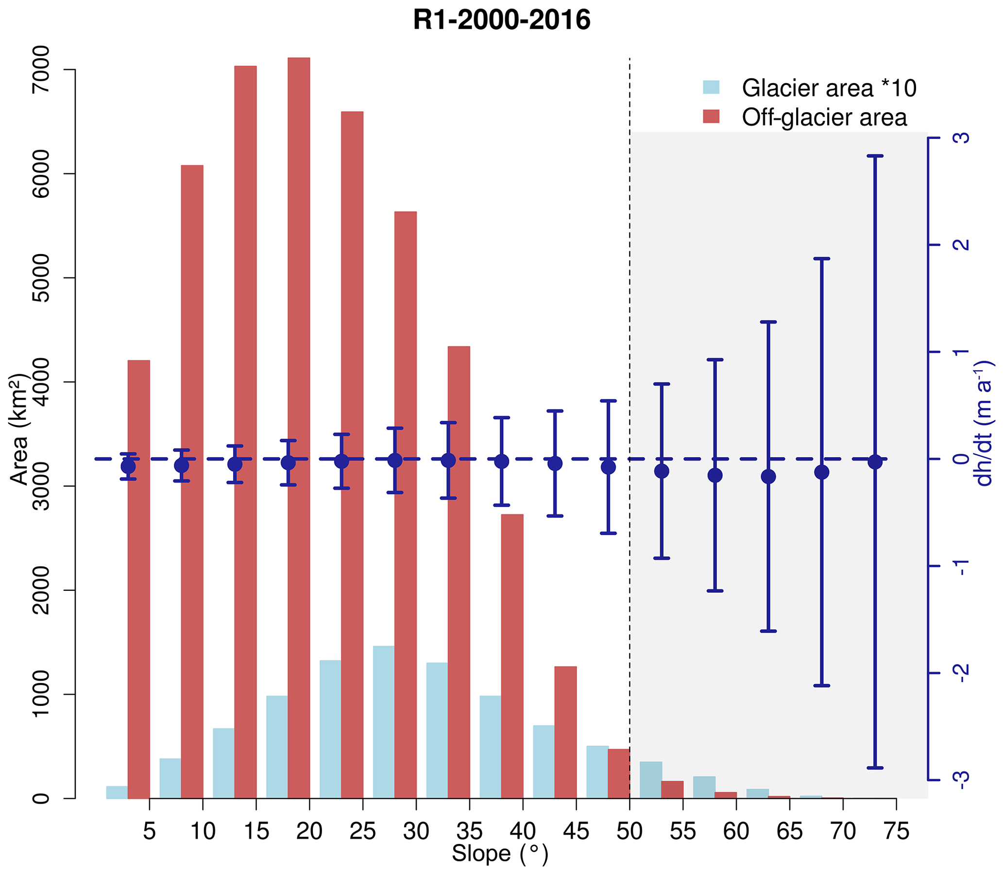
Figure 2Off-(red) and on-glacier (light blue) area and off-glacier elevation change (blue dots) distributions as a function of slope in subregion R1 for the period 2000–2016. Error bars represent NMAD of Δh∕Δt values in the individual slope interval. The dotted line indicates the applied slope threshold (see Sect. 4.2). Glacier area measurements are based on the glacier outlines from 2000. Note: for better representation, on-glacier areas are scaled by a factor of 10. Plots for other subregions are provided in the Supplement.
The uncertainties of the generated elevation change rates are assessed by evaluating the elevation change rates on non-vegetated stable off-glacier areas (water and vegetation masks; see above). The lowest and highest 2 % quantiles of the change rates are rejected to suppress the impact of processing artefacts and outliers. To account for the dependency of the offsets on the slope (Figs. 2 and S3 and S4), the deviations are binned in slope intervals of 5∘. Remaining outliers are removed by employing a 3*NMAD filter for each slope bin. Finally, the area-weighted standard deviations σAW based on the offsets in off-glacier areas and the slope distribution in glacier areas are calculated.
Since we integrate elevation change information over the glacierized area, spatial autocorrelation of the elevation change fields must be considered in the accuracy assessment. We estimated the uncertainty of the computed average elevation change rates (σΔh∕Δt) according to the approach of Rolstad et al. (2009):
where is the correlation area, Agl is the analysed glacier area, and σAW is the assessed accuracy of the elevation change rates (explained in the next paragraph). The correlation length (dcor) is obtained by generating semivariograms with 100 000 random samples of Δh∕Δt values on the off-glacier areas. A binning in 30 m distance intervals and a maximum distance of 20 km are applied. Spherical semivariogram functions are fitted to the data and an average correlation length of 387 m results from the analysed elevation change fields. Equation (1) is applied for each continuous glacierized area (icecap or connected glaciers) and the area-weighted average of the individual ice-covered areas is taken as the region-wide σΔh∕Δt.
The hypsometric extrapolation of elevation change information leads to an additional uncertainty that is hard to quantify. We employed the approach of Berthier et al. (2014). A scaling factor (we selected a factor of 2) is applied to σΔh∕Δt for the area fraction with hypsometric extrapolation of Δh∕Δt, in order to obtain the uncertainty of our region-wide average elevation change rates δΔh∕Δt.
4.3 Mass balances
The geodetic mass balances ΔM∕Δt of the analysed regions are computed according to Fountain et al. (1997) by multiplying the integrated elevation change rates by the average ice density (volume-to-mass conversion factor). We applied two density scenarios. The first scenario follows the suggestion of Huss (2013) for alpine glaciers and we applied an average density (ρ) of 850 kg m−3. For the second scenario, two different conversion factors of 600 and 900 kg m−3 are applied for ablation and accumulation areas, respectively (Kääb et al., 2012; Gardelle et al., 2012). The average equilibrium line altitude (ELA) (see Table S3 and below) of each subregion is used to distinguish between both glacier sections. As revealed by Huss (2013), the conversion factor can vary strongly. Following his findings, we applied an uncertainty of ±300 kg m−3 for the conversion factor for observation intervals shorter than 10 years and mass budgets lower than ±200 kg m−2 a−1 and an uncertainty of ±60 kg m−3 for all other cases (see Braun et al., 2019). Mass budgets of individual glaciers are only calculated for the constant density scenario.
In order to estimate the accuracy of the geodetic mass balances, the following error contributions are considered:
-
accuracy of the elevation change rates δΔh∕Δt
-
accuracy of the glacier outlines δS
-
uncertainty of the applied average ice density δρ
-
potential bias due to different SAR signal penetration Vpen∕Δt.
This leads to the following formula to calculate the error of ΔM∕Δt:
The assessments of δS and δΔh∕Δt are depicted in Sect. 4.1 and 4.2. The uncertainty contribution by potentially different SAR signal penetration in the glacier surfaces is evaluated following the approach of Malz et al. (2018). No difference in the SAR signal penetration in the ablation areas below the equilibrium line altitude (ELA) is assumed. These areas experience melt throughout the year in the tropical Andes (Kaser, 2001) and differences in the radar signal penetration in wet glacier surfaces are small (Casey et al., 2016; Rossi et al., 2016; Ulaby et al., 1984). A linear increase in the penetration depth bias towards 5 m between the ELA and the highest peaks is employed in the accumulation areas to calculate Vpen. Depending on the applied scenario, a volume-to-mass conversion factor of 850 or 600 kg m−3 is taken. The late summer snow line altitude (SLA) derived from optical satellite images is a good proxy for the ELA in the tropical Andes (Rabatel et al., 2012). Thus, the average ELA in the study period for the subregions is estimated based on published ELA and SLA values. Table S3 provides an overview of the considered ELA and SLA values. Uncertainties in the estimated ELA positions affect the penetration depth bias estimation and thus the error budget. A sensitivity analysis of an ELA mismatch on the error budget is provided in Braun et al. (2019). Specific mass balances are calculated according to the UNESCO Glossary of Glacier Mass Balance (Cogley et al., 2011) by applying the average glacier area of each observation period (mean glacier extent with slopes < 50∘).
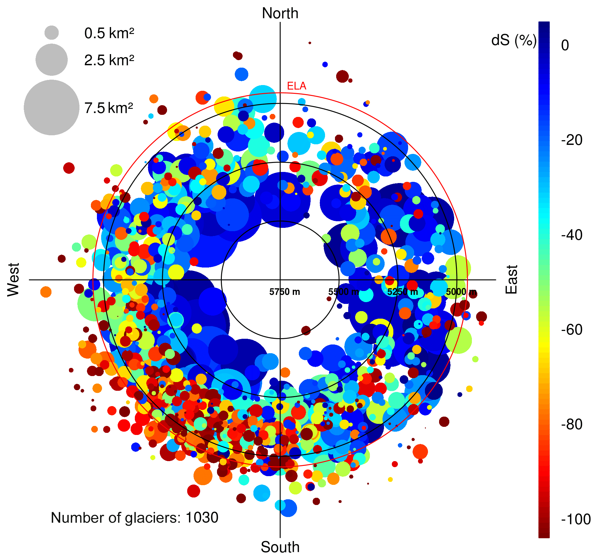
Figure 3Polar plot of relative area changes (dot colour) in subregion R1 in the period 2000–2016 of individual glaciers. Dot size: glacier size in 2000; radius: median elevation; orientation: mean aspect. Red circle: equilibrium line altitude (ELA); see also Table S3. Plots for other subregions and time intervals are provided in the Supplement.
5.1 Glacier inventory
The glacier outlines from 2000, 2013, and 2016 of some example mountain ranges from all three subregions are shown in Fig. S5. A clear recession of the glaciers in all subregions is obvious. The measured extents of the glaciers for all subregions and time steps are presented in Table 1. Since cloud and snow cover do not allow for a complete coverage of subregions R1 and R2 in 2013 and no suitable SAR data cover the debris-covered ice areas in the Cordillera Blanca in 2013, a small fraction of the glacier area (subregion R1: 2.1 %; subregion R2: 4.4 %) is mapped using imagery from 2014. For subregion R1, a nearly complete mapping (99.5 %) of the glacier areas in 2014 is possible. The obtained average area change rate between 2013 and 2014 at glaciers delimited in both years is employed to correct the area change measurement in subregion R1 for 2013 at glaciers only delimited in 2014 and vice versa. In subregion R2, the change rate between 2013 and 2016 is applied to perform a similar correction of the area change measurements in 2013. In total, ice covered areas of 1916.6±48.3 km2 in 2000, 1571.9±43.1 km2 in 2013, and 1368.1±45.5 km2 in 2016 are estimated for Peru. Based on the catchment divides of the RGI6.0, a reduction in the number of glaciers from 1973 in 2000 to 1803 in 2016 is observed. The variations in the glacier count and area in the subregions and in the whole country are summarized in Tables 1 and 2. It should be noted that the uncertainty of the area changes (Table 2) results from the uncertainty of the individual inventories (quadratic sum), assuming independence of the individual area measurements. The revealed area changes of individual glaciers in the different subregions and study periods are correlated with topographic parameters (glacier area, median elevation, mean aspect) and plotted in Figs. 3 and S6–S13.
Table 1Measured glacier extents for different years and regions.
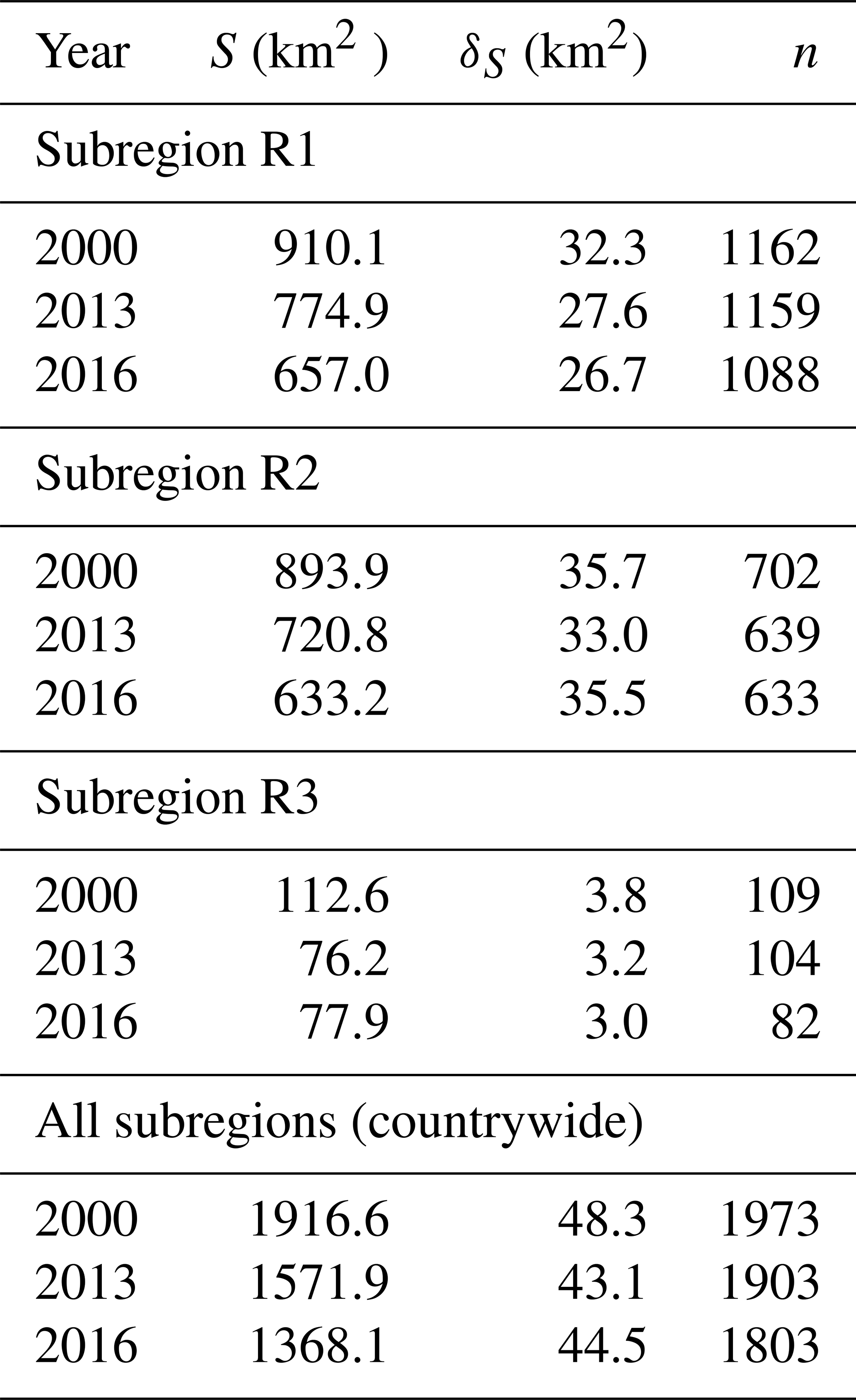
S: measured glacier area. δS: uncertainty of measured glacier area. n: number of glacier catchments (delineations based on RGI 6.0).
5.2 Elevation changes
The obtained unfiltered elevation change rates on ice-covered areas at some example mountain ranges are illustrated exemplarily in Figs. 4 and 5 for the periods 2000–2013 and 2013–2016, respectively. In the interval 2000–2013, a clear thinning of the lower glacier parts in the Cordillera Vilcanota and Apolobamba is observed. The glaciers in the Cordillera Blanca and Huayhuash show a more balanced pattern and Coropuna experienced thinning throughout most of its ice cap. An increase in the surface lowering rates at most mountain ranges is obvious in the interval 2013–2016. Only the ice caps in subregion R3 show reduced lowering rates. Since the TDX data in 2013 do not cover the whole glacier area in subregion R3, the voids are filled with TDX data from 2014. The glacier area covered by Δh∕Δt measurements using TDX data from 2014 amounts to only 1.4 % (glacier outlines from 2000). The impact of this void filling is considered negligible since the analysis uses change rates. The average measured and extrapolated surface elevation change rates of all subregions for different observation periods are listed in Table 2. The fraction of glacier area covered by Δh∕Δt measurements is lowest in subregion R1, when using the SRTM DEM as a reference (Table 2). Large data voids in the SRTM data lead to a partial coverage of only 46 % of the ice-covered area in subregion R1 in 2000 (61 % in subregion R2, 89 % in subregion R3). The number of measurements on the glacierized areas clearly increases when deriving the elevation change solely from TDX datasets (Table 2). In the period 2013–2016, a coverage of up to 80 %, 69 %, and 89 % is obtained in subregions R1, R2, and R3, respectively. Since the differential InSAR approach is used to generate the TDX DEMs, the proportion of areas affected by phase jumps in the unwrapped interferogram is small (∼1 % of the total glacier area). The major area affected by phase jumps (at the Cordillera Vilcanota in 2016) is highlighted in Fig. 5. Figures 4 and 5 indicate that the elevation change rates are altitude dependent. The hypsometric distributions of the measured elevation change rates and the respective ice-covered areas are plotted in Figs. 6, S14, and S15 for each subregion in the interval 2000–2016. Surface lowering is found on areas below 5700 m in subregion R1, 5800 m in subregion R2, and 5900 m in subregion R3. Considerable positive elevation changes are observed in the higher reaches of the glaciers in subregion R1. The obtained elevation change rates of the glaciated areas are available via the PANGAEA database (https://doi.org/10.1594/PANGAEA.906211, Seehaus et al., 2019).
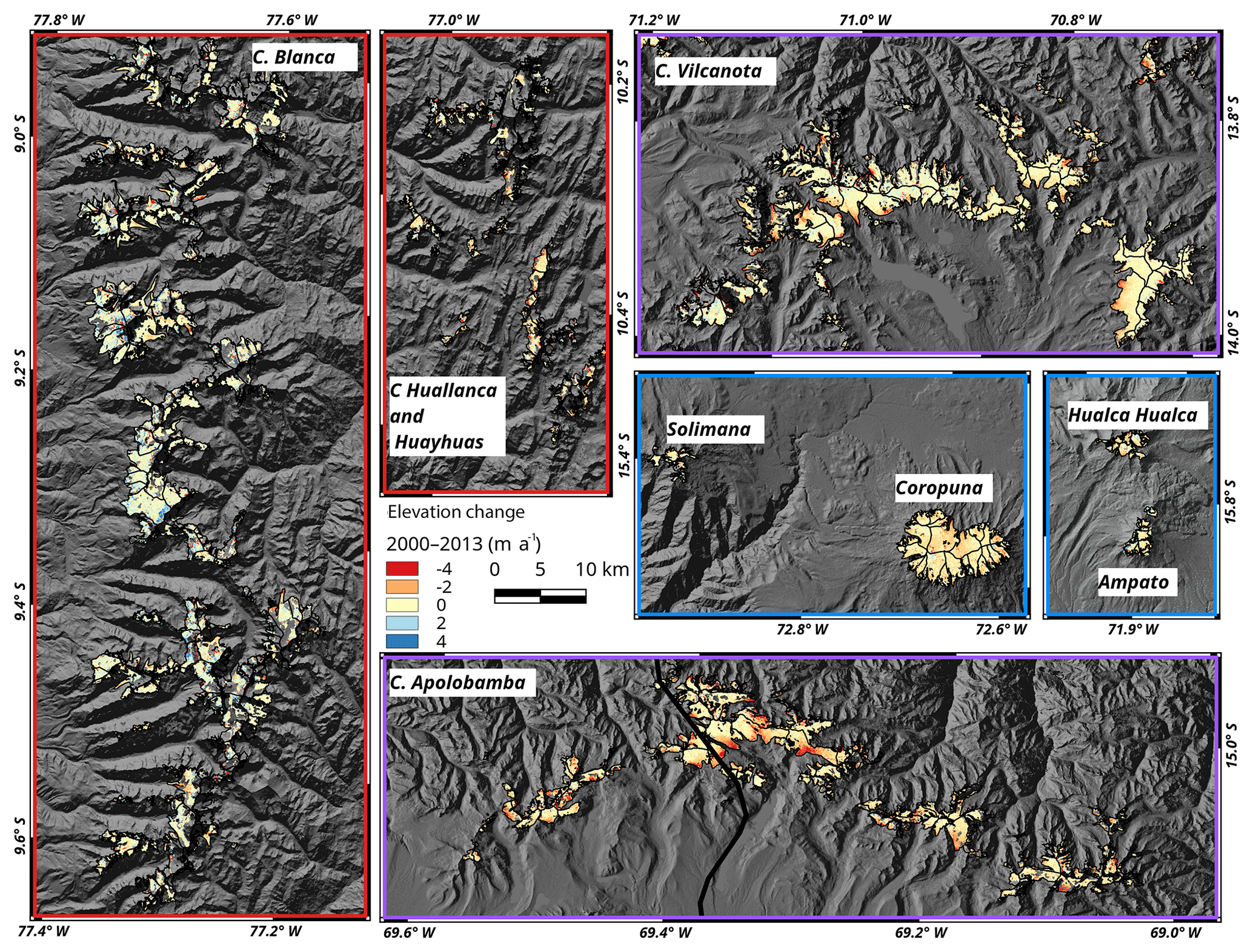
Figure 4Surface elevation changes in the period 2000–2013 at mountain ranges in all three subregions (unfiltered). The frame colour of the panels indicates the subregions (see Fig. 1). Background: SRTM DEM hillshade © NASA.
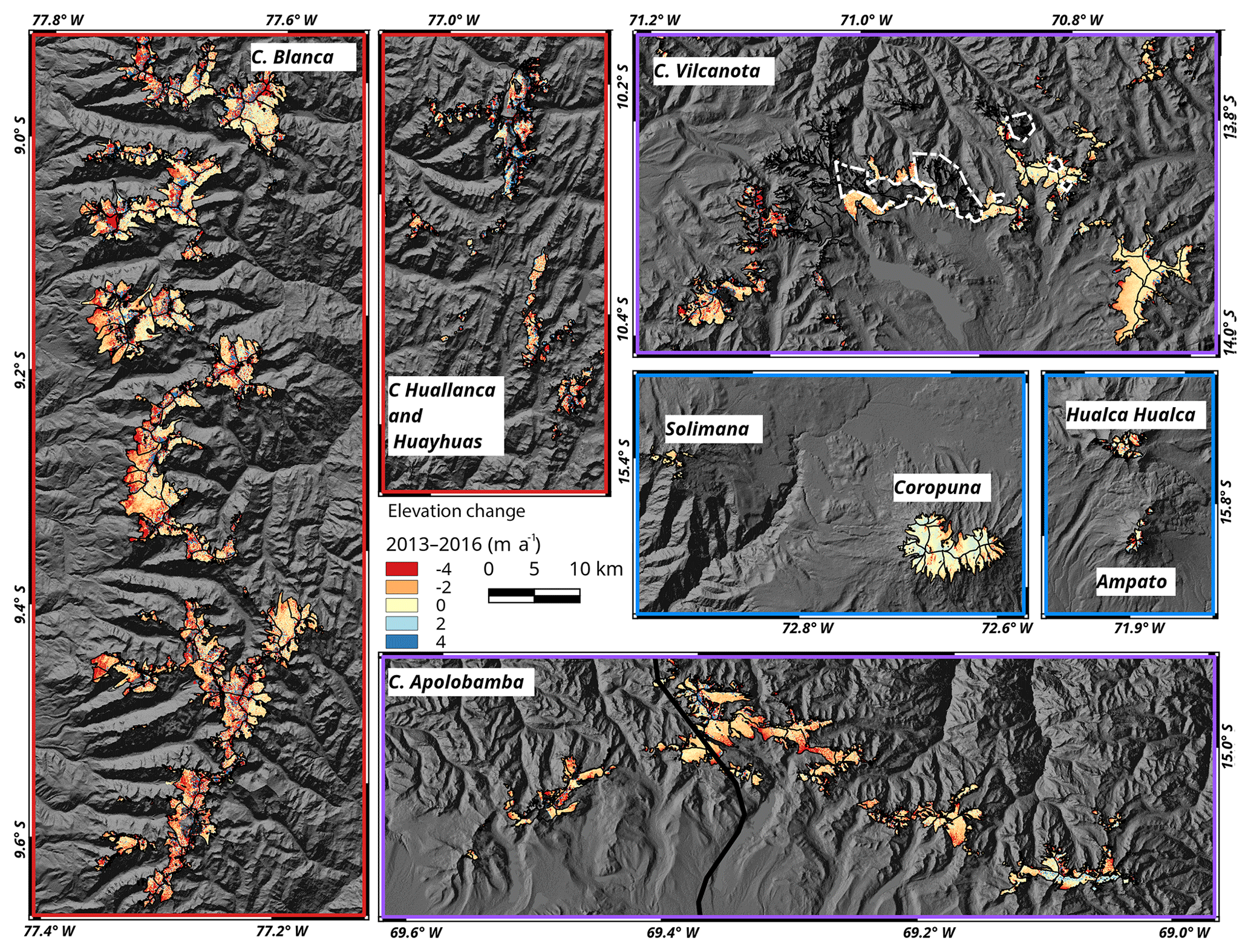
Figure 5Surface elevation changes in the period 2013–2016 at mountain ranges in all three subregions (unfiltered). The frame colour of the panels indicates the subregions (see Fig. 1). White dashed line: masked out areas affected by phase jumps in the unwrapped interferogram. Background: SRTM DEM hillshade © NASA.
Table 2Measured area, surface, and mass changes for different periods and regions. a Constant volume-to-mass conversion factor of 850 kg m−3. b Volume-to-mass conversion factor of 600 kg m−3 and 900 kg m−3 for region below and above the ELA (Table S3), respectively. c Mean glacier area of observation interval is used to calculate specific mass balances (see Sect. 4.3)
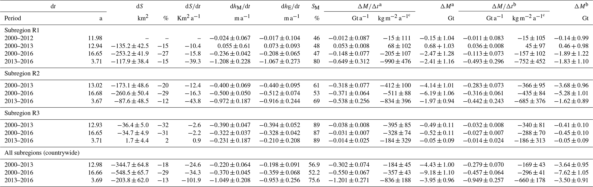
dt: observation period (mean time lag between DEM dates). dS: glacier area change. dS∕dt: glacier area change rate (mean time lag between glacier inventories is used). dhM∕dt: average measured surface lowering rate. dhE∕dt: average extrapolated surface lowering rate. SM: fraction of glacier area covered by dhM∕dt measurements (below slope threshold). ΔM∕Δt: mass balance (average and specific). ΔM: total mass change in the observation period.
5.3 Mass balances
The geodetic mass balances derived from the elevation change information of the individual subregions are listed in Table 2. In total, a mass loss of or Gt is found for Peru in the period 2000–2016, depending on the applied density scenario (Sect. 4.3). The mass loss rates show an increase between the observation periods 2000–2013 and 2013–2016. Only in subregion R3 is a slight reduction of the mass loss observed. The most prominent increase in glacier wastage is revealed in subregion R1. The mass budget changed from nearly stable conditions of 45±97 kg m−2 a−1 in 2000–2013 to a specific mass loss rate of kg m−2 a−1 in 2013–2016 (second density scenario). The computed mass balances of individual glaciers in the different subregions and study periods are correlated with topographic parameters (glacier area, median elevation, mean aspect) and plotted in Figs. 7 and S16–S20.

Figure 6Hypsometric distribution of measured (red bars) and total (light blue bars) glacier area with elevation in subregion R1 in the interval 2000–2016. Blue dots represent the mean Δh∕Δt value in each elevation interval. Error bars indicate NMAD of Δh∕Δt for each hypsometric bin. Grey areas mark the lower and upper 1 % quantile of the total glacier area distribution. Black dashed line: mean glacier elevation; red dashed line: equilibrium line altitude (ELA); see also Table S3. Area measurements are based on the glacier outlines from 2000, considering only regions with slopes below applied slope threshold (50∘; see Sect. 4.2). Plots for other subregions are provided in the Supplement.
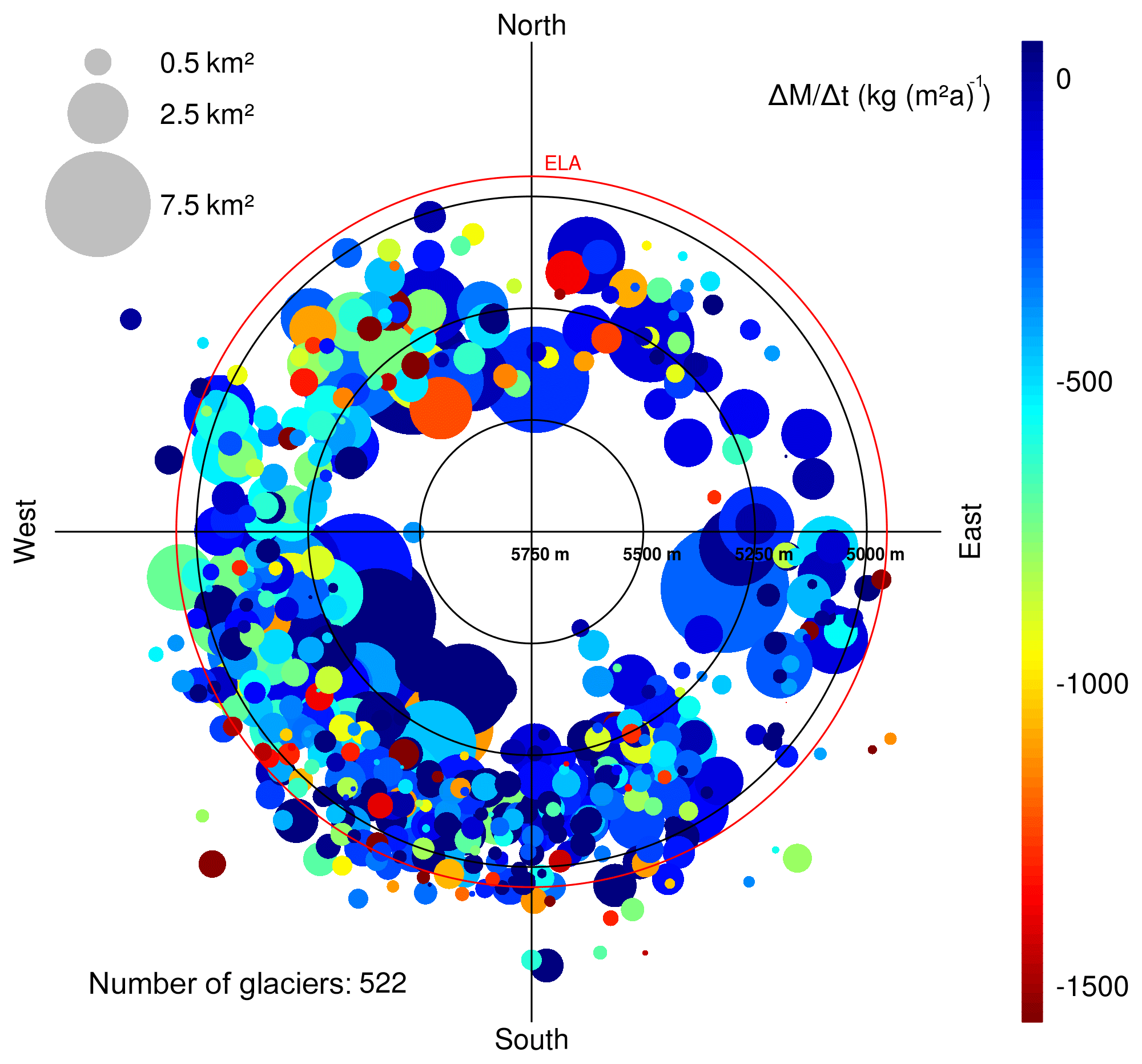
Figure 7Polar plot of specific mass balance (dot colour) of individual glaciers in subregion R1 in the period 2000–2016 of individual glaciers. Dot size: glacier size in 2000; radius: median elevation; orientation: mean aspect. Red circle: equilibrium line altitude (ELA); see also Table S3. Note: only glaciers with elevation change information > 50 % are included. Plots for other subregions and time intervals are provided in the Supplement.
6.1 Glacier retreat
We observed a dramatic recession of the glaciers throughout Peru of −29 % ( km2; −1.8 % a−1) between 2000 and 2016. Our total mapped glacier extent of 1368.1±44.5 km2 in 2016 is comparable to the reported coverage of 1298.6 km2 by the recent Peruvian glacier inventory (UGRH, 2014), considering that UGRH did not include the glacier areas of the Bolivian Cordillera Apolobamba (∼70 km2 ). The glacier area mapped in the RGI6.0 amounts to 1602.96 km2, which is in the range of our measurements for 2000 and 2013. A direct comparison is complex since the RGI6.0 is a blended product with outlines discriminated between 2000 and 2009 in Peru. However, visual inspection of our outlines and the RGI6.0 revealed that numerous small glaciers (especially in the southern section of subregion R1 and throughout the whole subregion R3) mapped in the RGI6.0 are artefacts, which are caused most probably by temporary snow cover. This issue has already been mentioned in the RGI Technical Report (RGI Consortium, 2017). Thus, our glacier inventory of Peru in 2000 has 350 fewer features than the RGI6.0. By contrast, the Peruvian glacier inventory (UGRH, 2014) lists 2679 glaciers. This difference can be explained by the different basin delineations applied.
The comparison of our area measurement of 1916.6±48.3 km2 in 2000 and the first Peruvian glacier inventory (Hidrandina SA, 1989) in 1970 (2041.85 km2) results in a retreat of −7 % (−139.9 km2; 0.2 % a−1). However, not all cordilleras were mapped completely by the first Peruvian glacier inventory. When considering only the glacierized cordilleras which were completely mapped in the first Peruvian glacier inventory (UGRH, 2014), the area changes amount to −23 %. Figure 8 illustrates the temporal evolution of the glacier area changes and highlights that Peru's glaciers have experienced long-term shrinkage since 1970 with increasing rates in recent years. This observed trend is in accordance with the findings of previous studies at individual mountain ranges. Silverio and Jaquet (2017) summarized area measurements of several studies in the Cordillera Blanca (subregion R1) and revealed an increase in the loss rate from about −5 km2 a−1 between 1971 and 1996 towards −23 km2 a−1 between 2014 and 2016. Burns and Nolin (2014) reported a ∼3.5 times higher area loss rate in 2004–2010 compared to 1970–2003 in the Cordillera Blanca. Area loss rates of ∼1.8 % a−1 (> 50 %) since 1975 are reported by the Instituto Geofisico del Peru (2010) and López-Moreno et al. (2014) for the Cordillera Huaytapallana, which is higher than our finding of −1.1 % a−1 in subregion R1 in the period 2000–2013. However, their study period includes strong El Niño events in the 1980s and 1990s (Fig. 8), which typically lead to increased glacier melt in the tropical Andes (Wagnon et al., 2001). Retreat measurements in subregion R2 are carried out at the Cordillera Vilcanota (Hanshaw and Bookhagen, 2014; Salzmann et al., 2013; Veettil and Souza, 2017), the Cordillera Apolobamba (Cook et al., 2016; Veettil et al., 2017a), the Cordilleras Carabaya, Urubamba, and Vilcabamba (Veettil et al., 2017d), and at glaciers draining into the Vilcanota–Urubamba basin (Drenkhan et al., 2018). All studies revealed significant glacier shrinkage since the 1980s with retreat rates in the range of −0.9 to −1.7 % a−1. These findings are comparable with our observed rate of −1.3 % a−1 in subregion R2 in the period 2000–2013. Drenkhan et al. (2018) revealed reduced shrinkage rates for 2010–2016 compared to 2004–2014. This is contradictory to our observed strong increase in glacier recession after 2013. They analysed only glaciers in the Vilcanota–Urubamba basin, of which most face south. We measured the highest retreat for glaciers facing north in subregion R2 in the period 2013–2016 (Fig. S22) and only low retreat for south-facing glaciers. Thus, different spatial extents and representativeness of topographic attributes in the analysed regions leads to the mismatch of the observed retreat trends. Moreover, this suggests that the representativeness of topographic settings needs to be considered when doing region-wide upscaling of sampled glacier change measurements. At the ice cap of the Coropuna volcano (subregion R3), various ice coverage estimates are available going back to 1955 (Peduzzi et al., 2010; Racoviteanu et al., 2007; Silverio and Jaquet, 2012; Ubeda, 2011; Veettil et al., 2016). The average loss rate of ∼1.5 % a−1 (1955–2015) is lower than our estimated rate of −2.3 % a−1 for subregion R3 in the period 2000–2013. In addition to differences in the study periods, we attribute this deviation to the fact that our estimate for subregion R3 includes numerous small glaciers located at lower altitudes (Fig. S10). These glaciers are in general more sensitive to climate change (Francou Bernard et al., 2003; Vuille et al., 2008) in comparison to the more elevated glaciers of the Coropuna volcano. Moreover, Veettil et al. (2016) discovered an increased retreat and uplift of the SLA after ∼2000 at Coropuna's ice cap, supporting our findings.
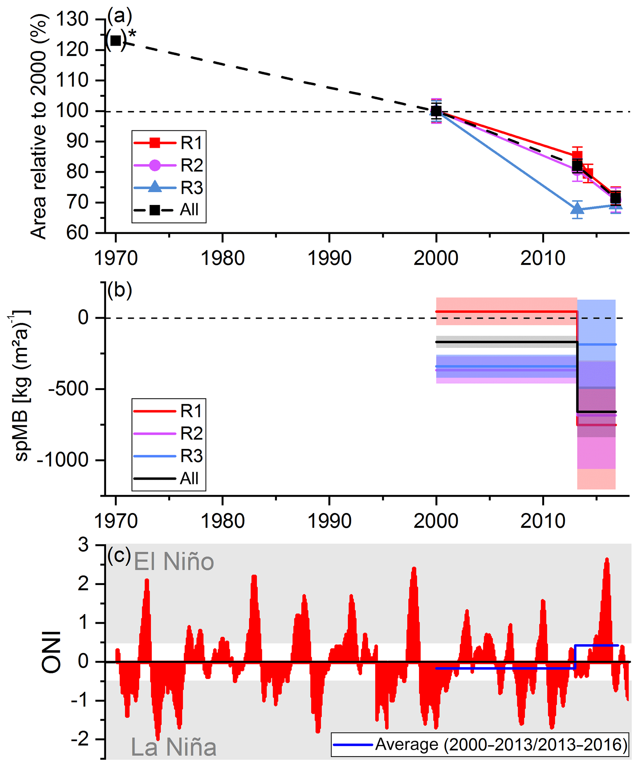
Figure 8Temporal evolution of (a) relative glacier area changes, (b) observed specific mass balance (spMB; colour shaded areas represent the uncertainty of the corresponding measurements), and (c) Oceanic Nino Index (ONI) in the period 1970–2016. * Area measurement in 1970 taken from the first Peruvian glacier inventory (Hidrandina SA, 1989) and only mountain ranges with complete coverage by the inventory in 1970 are considered in the area change computation (see also Sect. 6.1).
For the period 2013–2016, we discovered a 4 times higher countrywide retreat rate compared to the period 2000–2013. The strongest increase is found in subregion R2, whereas in subregion R3 (only ∼5 % of total glacier area) the glacier area remained quite stable after 2013. The increased retreat rates in subregions R1 and R2 after 2013 can be attributed to the strong ENSO activities in the years 2015–2016. An average ONI of 0.42 is reported for 2013–2016 and the maximum ONI of 2.6 in December 2015 indicates distinct El Niño conditions. On the other hand, an average ONI of −0.17 is revealed for 2000–2013, indicating that La Niña conditions dominated this period. Since El Niño periods typically lead to increased glacier wastage in the tropical Andes (e.g. Vuille et al., 2008; Wagnon et al., 2001) (Sect. 2), our observed increased shrinkage after 2013 can be attributed to the ENSO activities in this period. This pattern also fits the findings by Morizawa et al. (2013) (Condoriri Glacier, Bolivia) and Silvero and Jaquet (2017) (Cordillera Blanca, subregion R1). Both studies reported enhanced recession during El Niño events and even area gains during La Niña epochs. The latter study also discovered a linear relation between glacier retreat and ONI (R2=0.8) and reports a change rate of −5 % a−1 for 2014–2016 that is equal to our change rate at subregion R1 for 2013–2016. Moreover, the glaciers in the tropical Andes are on average the thinnest worldwide (Farinotti et al., 2019). Therefore, the increased melt will lead to more pronounced changes in the glacier area compared to other glacier regions. The stagnation of the glacier retreat in subregion R3 in the interval 2013–2016 is difficult to explain. During the strong El Niño in 1997/98, increased precipitation was observed at the Coropuna volcano in subregion R3 (Herreros et al., 2009; Silverio and Jaquet, 2012), whereas El Niño usually leads to reduced precipitation rates. Veettil et al. (2016) reported positive precipitation anomalies after 2011 and clearly negative anomalies in the period 2009–2011 for the Coropuna volcano. However, the total precipitation data from ERA-Interim indicate lower precipitation rates after 2013 (Fig. S24) and do not clearly indicate an increase in precipitation during El Niño 1997/98. Since the small glacier areas in subregion R3 cover mainly volcano peaks, the revealed precipitation values from the spatially coarse ERA-Interim data do not necessarily reflect the local precipitation pattern at the prominent, high-altitude volcano peaks. Additionally, the mean glacier altitude in 2013 shifted ∼100 m above the ELA (Fig. S25), whereas the mean glacier altitude in 2000 was nearly similar to the ELA (Fig. S15). A significant temporary snow cover at the non-glacierized Cordillera del Barroso (subregion R3, close to the boarder to Bolivia) was observed during the dry seasons in 2015 and 2016 (Lèon et al., 2019), which fits to the suggested increased precipitation at high elevations after 2013. Moreover, snowfall events during the dry season strongly affect the glacier albedo and thus lead to reduced ablation. However, the temporary snow cover during the dry season in 2016 in subregion R3 might have also affected the mapping of the glacier outlines. Although only imagery with no or only minimal snow coverage is selected, it is quite likely that some remaining snow cover was located at the glacierized peaks, leading to a slightly larger glacier area in 2016 compared to 2013. This bias is not quantifiable and certainly within the range of applied uncertainty. Thus, we conclude that the glacier area did not significantly change in subregion R3 after 2013 and attribute this to the allocation of the remaining ice at higher altitudes and increased precipitation, especially during the dry season, even though a strong El Niño event occurred in this period.
The analysis of area fluctuations of individual glaciers revealed in all three subregions indicates higher recession for glaciers with lower median elevation and for small glaciers (Figs. 3 and S6–S13). This is in accordance with findings reported in previous studies (e.g. Kaser and Osmaston, 2002; Mark and Seltzer, 2005; Ramirez et al., 2001). Small glaciers have in general a more narrow altitude range compared to larger glaciers, which can maintain the ELA below the maximum glacier elevation. A rise in SLA (a proxy of the ELA in the tropical Andes, Sect. 4.3) is observed throughout the Peruvian Andes by various studies (Hanshaw and Bookhagen, 2014; López-Moreno et al., 2014; McFadden et al., 2011; Veettil et al., 2016, 2017c, d). This corresponds to our observed retreat pattern. Figures 3 and S6–S13 suggest that glaciers with slopes facing on average the south-south-west direction experienced in general higher relative retreats. The total amount of lost glacier area repeats this general pattern (Figs. S21–S23). This can be attributed to the fact that more low-lying, small glaciers with mean aspects facing southwards still exist (Figs. 3 and S6–S13). Higher retreat rates in general were observed for north-orientated glaciers before 2000 (Veettil et al., 2017a; Veettil, 2018), leading already to the disappearance of small north-facing glaciers before the start of our observation periods.
In total, we discovered that 177 glaciers had disappeared in our observation period, of which most disappeared after 2013 and were south facing (Table 1 and Figs. S11–S13). At the Artesonraju Glacier in the Cordillera Blanca (subregion R1), Vuille et al. (2018) projected an uplift of the ELA by 300–700 m until 2100 based on the CMIP5 scenarios RCP4.5 and RCP8.5. Thus, the proceeding climate change will lead to the further disappearance of numerous small low-lying glaciers in the tropical Andes within the next decades, as predicted by Ramirez et al. (2001) and Huh et al. (2017).
The gain and formation of proglacial lakes are consequences of glacier recession (Cook and Quincey, 2015) and increase the GLOF risk of downstream areas. Veettil et al. (2017a) discovered an increase in the number of glacial lakes from 697 to 903 in the Cordilleras Apolobamba and Carabaya between 1985 and 2015. In the Cordillera Vilcanota, Hanshaw and Bookhagen (2014) observed stable or increasing extents in 77 % of the lakes connected to glacial watersheds. Colonia et al. (2017) compiled an inventory of 201 potential future glacier lakes based on modelled glacier bed overdeepenings. Considering the revealed findings by this study as well as previously reported values and projections, a further region-wide monitoring of glacier retreat and lake development is highly advisable to identify potential GLOF risks in the tropical Andes, as also suggested by Cook et al. (2016).
6.2 Surface elevation changes and mass balances
The average countrywide glacier surface elevation change between 2000 and 2016 amounts to m a−1, which corresponds to a specific mass budget of or kg m−2 a−1 depending on the applied density scenario. The second density scenario leads to 8 %–21 % lower countrywide mass balances. As pointed out by Kääb et al. (2012), this scenario is suitable for glaciers with no dh∕dt due to ice dynamics and when dh∕dt is clearly driven by melt or increased accumulation. Since these conditions are typical for the Peruvian glaciers (see Sect. 1 and further down), we used the results of the second density scenario for further discussion and analyses. On the other hand, the results from the first scenario provide suitable information for comparison with other studies. Moreover, using the second scenario reduces the potential bias by the SAR signal penetration depth differences (Sect. 3) on the mass budget by ∼40 % compared to the first scenario. A computation of individual glacier mass balances using the second scenario is not performed due to the lack of ELA information on glacier scales.
The highest average surface lowering is revealed for subregion R1 in the period 2013–2016 (Table 2). However, the stable surface elevations before 2013 in subregion R1 suppress the long-term average value. The nearly balanced budget contradicts the observed glacier retreat of −15 % in subregion R1 in the interval 2000–2013 at first glance. The mean surface elevation change in the retreat areas amounts to −0.28 m a−1, clearly indicating mass loss in the deglacierized areas. However, elevation gain is found at high altitudes. The more La Niña-like conditions of ENSO in the period 2000–2013 (Sect. 6.1) and an increase in precipitation in this region due to stronger upper-tropospheric easterlies (Schauwecker et al., 2017) have most probably led to higher accumulation rates. ERA-Interim reanalysis data also show an increase in total precipitation in this period, especially around 2007 (La Niña event). Thus, the accumulation gain in the upper reaches balanced the ice losses at the termini, even though temperatures increased (Schauwecker et al., 2017). In all subregions an increase in temperature is found in the reanalysis data for 2000–2013, but the strongest positive precipitation anomaly is found in subregion R1 (Figs. S24 and S26). This explains the mass losses in subregions R2 and R3 in this period.
Skin temperature was still above the long-term average in subregions R1 and R2 after 2013 (Fig. S26). The downward surface thermal radiation shows an increase in subregion R1 (Fig. S27), whereas total precipitation decreased in subregion R2 and remained nearly stable in subregion R1 (Fig. S24). Those climatic variations enhance the ablation and facilitate a positive feedback that further increases the glacier melt. The higher temperature as well as reduced and delayed precipitation, which are typical during El Niño, lead to liquid precipitation in the ablation regions and a reduced glacier albedo, enhancing the short-wave radiation absorption (e.g. Vuille et al., 2018; Maussion et al., 2015). Thus, the climatic variations explain the more negative mass balances in both subregions in the period 2013–2016, which also correlate with the strong El Niño activities in this interval (Fig. 8).
Only at subregion R3 did the thinning rate reduce after 2013, although El Niño conditions dominated. We attribute this, like the stable glacier area, to higher precipitation rates, especially during the dry season, at the ice-capped volcanos and the allocation of the remaining ice masses at high elevations (see Sect. 6.1 for more details). Moreover, the revealed spatial pattern of mass balances after 2013, with the highest mass loss rates at the northernmost subregion R1 (Table 2), matches the observed trend of higher river runoff towards northern Peru during strong El Niño events (Casimiro et al., 2012, 2013).
The analysis of the mass balance of individual glaciers and topographic parameters in subregions R2 and R3 reveals a trend towards higher mass losses for glaciers facing north-north-east in the period 2000–2016 (Figs. 7, S16, and S17). This trend agrees with observations by Soruco et al. (2009a) in the Bolivian southern wet outer tropics. In the interval 2000–2016, no clear dependency of the specific glacier mass balances on the median elevation or aspect is obvious in subregion R1 (Fig. 7). However, Fig. 5 suggests a trend towards higher surface lowering rates on the western slopes of the Cordillera Blanca in the period 2013–2016. The subregion-wide analysis of glacier elevation changes as a function of aspect does not reveal any clear trend (Fig. S28); however, when analysing only the Cordillera Blanca an east-to-west gradient is obvious (Fig. S29). We attribute this to the changed precipitation pattern during El Niño. Higher precipitation rates are typically found on east-facing slopes at the Cordillera Blanca, fed by moist air from the Amazon basin (Garreaud et al., 2009). However, during El Niño the westward flow of moist air is hampered by stronger westerlies (Vuille, 2013), which increases the precipitation gradient across the Cordillera Blanca.
Long-term glaciological mass balance measurements are only available for two glaciers (WGMS, 2018). For the Artesonraju and Yanamarey glaciers, both located in subregion R1, average mass budgets of −911 and −1.491 km m−2 a−1 (2013–2016) are revealed from field measurements, whereas we observed and kg m−2 a−1, respectively. Both methods show higher loss rates for the Yanamarey Glacier compared to the Artesonraju Glacier. The deviation of ∼50 % between both approaches at Yanamarey Glacier (overlap within the error range) can be partly attributed to different observation intervals and basin delineations. Moreover, glaciological mass balance measurements are typically based on some stake measurements in the lower, often most accessible, ablation zone and only a few measurements in the accumulation region. At the Zongo Glacier, Bolivia, Soruco et al. (2009b) performed a comparison of different mass balance methods (glaciological, hydrological, and geodetic) and revealed a strong offset in the glaciological mass balance estimates. The authors suggest that the limited number of field measurement points is not representative of the whole glacier and that the interpolation between the measurement sites can bias glacier-wide specific mass balance information. On the other hand, to obtain glacier-wide mass balance estimates using the geodetic method, there is interpolation over data voids in the elevation change fields needed (in our case we used the hypsometric elevation change distribution). Thus, we attribute the offset between the results from both methods to uncertainties due to interpolation, spatial sampling and different observation periods.
The correlation of the annual glaciological measurements with the average ONI of the respective observation periods indicates a trend towards increased mass loss and higher ELA during El Niño conditions (Fig. S30). These tendencies fit with the observations by Silvero and Jaquet (2017) and Morizawa et al. (2013) (see Sect. 6.1) and support our revealed correlation between the increased glacier wastage in the period 2013–2016 and the strong El Niño event during this period.
Since the highest density of glaciological point measurements are collected at the lowest section at both glaciers and considering the observation of Soruco et al. (2009b) at Zongo Glacier, Bolivia, that the terminus region strongly dominates the mass balance variations in a tropical glacier, we did an analysis of the glaciological mass balance at regions below 4900 and 5000 m a.s.l. at Yanamarey and Artesonraju glaciers, respectively. A trend toward increased mass losses after 2011 is obvious (Fig. S31, unfortunately the data at Yanamarey Glacier for the period 2009–2011 were incomplete), fitting with the revealed more negative geodetic mass balances after 2013. Moreover, the most negative values are derived for the period 2015–2016, which also supports our suggestion that ENSO forced the increased glacier wastage after 2013. The comparison between the geodetic and the average glaciological measurements at the terminus regions in the period 2013–2016 revealed a good agreement of both methods at Yanamarey Glacier (average glaciological: −3152 kg m−2 a−1; geodetic: −3164 kg m−2 a−1), whereas at Artesonraju Glacier, the geodetic measurements indicate higher mass loss (average glaciological: −4206 kg m−2 a−1; geodetic: −2696 kg m−2 a−1). This difference can be partly attributed to the different glacier basin definitions and slightly different observation intervals, but also to limitations of the individual methods, as discussed above.
In subregion R1, Huh et al. (2017) derived volume losses ranging from −0.019 to −0.150 km3 at six glaciers in the Cordillera Blanca from various elevation datasets in the period 1962–2008. This ice depletion corresponds to surface lowering rates of −0.20 to −1.4 m a−1. Mark and Seltzer (2005) reported lowering rates ranging from −0.14 to −0.59 m a−1 for three glaciers at the Nevado Queshque (Cordillera Blanca, subregion R1) in the interval 1962–1999. The findings of both studies are in the range of our revealed elevation change rates for subregion R1 of and m a−1 in the periods 2000–2016 and 2013–2016, respectively.
In subregion R2, Salzmann et al. (2013) estimated an ice volume loss in the Cordillera Vilcanota of ∼40 %–45 % between 1962 and 2006 based on ice thickness derived from glacier inventory parameters and thickness–volume scaling. The authors pointed out that nearly all ice loss occurred after 1985, leading to a lowering rate of about −0.39 m a−1 for the period 1985–2006. This value is similar to our measured average surface lowering in subregion R3 of m a−1 in the interval 2000–2013.
At the Coropuna volcano in subregion R3, Racoviteanu et al. (2007) measured an average glacier surface lowering of −5 m (−0.1 m a−1) based on a SRTM DEM and digitizing of a topographic map from 1955. Peduzzi et al. (2010) calculated a mean surface lowering of m a−1 for the period 1955–2000 and 1955–2002. Our revealed average surface lowering of m a−1 at the ice cap of the Coropuna volcano indicates an increased glacier wastage after 2000, which correlates with the increase in glacier retreat and SLA uplift observed by Veettil et al. (2016) since 2000.
The continent-wide surface mass balance simulation by Mernild et al. (2017) revealed an average mass change of kg m2 a−1 for the Andes north of 27∘ S in the epoch 2000–2014, which is much higher than our countrywide average of kg m2 a−1 for the period 2000–2013. This large offset can only be partly explained by the different study domains, time intervals, and glacier inventories applied and could be caused by limitations in the applied statistical downscaling of global circulation data.
On the countrywide scale, we observed ∼19 % less mass loss than Braun et al. (2019) (Region 02-04) in the period 2000–2012/13 (first density scenario). However, their analysis also includes the glacier areas in Bolivia, like the Cordillera Real, where significant glacier wastage is reported (e.g. Soruco et al., 2009a), leading to higher average mass loss rates. The change rates of subregions R1 and R2 in the period 2000–2012/13 and the results of Braun et al. (2019) in Regions 02 and 03 show good agreement, even though they are based on different glacier inventories. However, we computed more negative mass budgets in subregion R3 compared to Braun et al. (2019) (Region 04). This can be partly explained by the differences in the region delineation. Braun et al. (2019) included the few ice-covered volcanoes in south-west Bolivia. However, a more considerable reason for this offset is the fact that we found the highest number of misclassified ice-covered areas in RGI 6.0 in this subregion (Sect. 6.1). This explains the bias toward lower mass loss rates in the results of Braun et al. (2019), who measured surface elevation changes based on RGI 6.0. In a continent-wide analysis of geodetic mass budgets, like that of Braun et al. (2019), it is beyond the scope of the studies to map glacier outlines fitting to the whole elevation database as well. However, the revealed offset suggests the inaccuracy caused by imprecise glacier outlines and highlights the need for large-scale temporally consistent glacier outlines.
Gardner et al. (2013) carried out a comprehensive worldwide estimate of the glacier contribution to sea level rise. They computed a mass budget of kg m−2 a−1 (2003–2009) at the low latitudes (RGI region definition) by means of the extrapolation of glaciological measurements. A nearly similar value of m w.e. a−1 ( kg m2 a−1) is revealed by Zemp et al. (2019) by upscaling of glaciological and geodetic mass balances for the period 2006–2016. Both studies reported ice loss rates that are about 3 times higher than our countrywide average of kg m−2 a−1 (2000–2016). However, they are based on very few measurements (e.g. < 2 % spatial coverage for Zemp et al., 2019) in this region, resulting in the large uncertainties. Moreover, the representativeness of the settings of the sampled glaciers, which is not assessed, can also strongly influence region-wide estimates as discussed in Sect. 6.1. A comparison with GRACE measurements by Jacob et al. (2012) is also difficult since their spatial domain covers the whole of South America, only excluding Patagonia. Thus, the mass balance of the Peruvian glaciers cannot be disentangled from their results. These factors depict the limitations of using the present global mass balance estimates at the country or even mountain range level.
The above-mentioned global or countrywide estimates do not cover multiple periods and thus do not provide any information on temporal variability of the mass balances. Our analysis reveals strong temporal variations in the glacier changes that correlate with changing climate conditions and specific climatic events. These findings underline that mono-temporal analysis, especially when using short time intervals, can be biased by short-term climate anomalies like El Niño and highlights the need for further monitoring of the proceeding glacier recession in the tropical Andes.
The glaciers throughout Peru are strongly affected by changing climatic conditions, leading to considerable ice losses. In this comprehensive study we revealed a glacier recession of km2 (−29 %) in the period 2000–2016 and negative regional mass budgets of up to kg m−2 a−1 (northern wet outer tropics; 2013–2016). A strong increase in the countrywide mass and area loss rates from kg m−2 a−1 and −1.4 % a−1 in the period 2000–2013 to kg m−2 a−1 and −4.3 % a−1 in the interval 2013–2016 is shown. This amplified glacier wastage can be attributed to the strong El Niño in 2015/16. Spatial and temporal differences of the change rates of the studied subregions correlate with skin temperature and total precipitation trends derived from ERA-Interim reanalysis data and reported regional climatic variations. The analysis of area changes of individual glaciers indicates that the highest relative area change rates are found for low-lying and small glaciers, validating the prediction of the disappearance of numerous small glaciers located at low altitudes in the tropical Andes.
Our results provide the first multi-temporal region-wide and spatially detailed analysis covering all glacierized areas in Peru, providing fundamental data for projecting future glacier changes, water resource management schemes, and further glacier monitoring. The observed changes highlight the dramatic progression of glacier recession throughout Peru, which will lead to considerable socio-economic issues in this region. The increasing GLOF risk, due to the gain and formation of glacial lakes is just one aspect. The future contribution of glacier meltwater to the regional runoff puts the continuous water availability for irrigation, mining, hydropower generation, and drinking water supply, especially during the dry season, at risk. Therefore, we highly advocate resuming and further extending the glacier monitoring in the tropical Andes, not solely to gain scientific knowledge, but also to provide important information for local authorities and decision makers regarding water resource management and civil protection.
Elevation change fields are available via the World Data Center PANGAEA operated by AWI Bermeerhaven (https://doi.org/10.1594/PANGAEA.906211, Seehaus et al., 2019). Glacier outlines and glacier-specific results are available via the World Glacier Monitoring Service and GLIMS.
The supplement related to this article is available online at: https://doi.org/10.5194/tc-13-2537-2019-supplement.
TS designed and led the study, processed and analysed the data, and wrote the paper. TS, PM, and CS jointly developed the analysis routines for elevation change and mass balance computations. SL performed the SAR coherence computations. AC contributed to the interpretation of the data and provided field measurements. MB initiated and supervised the project. All authors revised the paper.
The authors declare that they have no conflict of interest. The founding sponsors had no role in the design of the study; in the collection, analysis, or interpretation of data; in the writing of the paper; or in the decision to publish the results.
The authors would like to thank the German Aerospace Center for providing TanDEM-X and TerraSAR-X data free of charge under AO XTI_GLAC0264 and AO ARC_HYD1763. Landsat data were kindly provided via USGS Earth Explorer and Sentinel-1 data were provided by ESA via Copernicus Open Access Hub. SRTM data were provided by NASA LP DAAC. Moreover, we would like to thank Christian Huggel and Duncan J. Quincey for reviewing and Francesca Pellicciotti for editing the paper.
This research has been supported by the Bundesministerium für Wirtschaft und Energie (grant no. 50EE1544 GEKKO), the Deutsche Forschungsgemeinschaft (the priority programme “Regional Sea Level Change and Society” SPP 1889 grant no. BR2105/14-1, the priority programme “Antarctic Research with comparative investigations in Arctic ice areas” SPP 1158 grant BR2105/9-1 and grant BR2105/13-1), and the Helmholtz Association (Alliance Remote Sensing & Earth System Dynamics).
This paper was edited by Francesca Pellicciotti and reviewed by Christian Huggel and Duncan J. Quincey.
Atwood, D. K., Meyer, F., and Arendt, A.: Using L-band SAR coherence to delineate glacier extent, Can. J. Remote Sens., 36, S186–S195, https://doi.org/10.5589/m10-014, 2010.
Baraer, M., Mark, B. G., McKenzie, J. M., Condom, T., Bury, J., Huh, K.-I., Portocarrero, C., Gómez, J., and Rathay, S.: Glacier recession and water resources in Peru's Cordillera Blanca, J. Glaciol., 58, 134–150, https://doi.org/10.3189/2012JoG11J186, 2012.
Berthier, E., Vincent, C., Magnússon, E., Gunnlaugsson, Á. Þ., Pitte, P., Le Meur, E., Masiokas, M., Ruiz, L., Pálsson, F., Belart, J. M. C., and Wagnon, P.: Glacier topography and elevation changes derived from Pléiades sub-meter stereo images, The Cryosphere, 8, 2275–2291, https://doi.org/10.5194/tc-8-2275-2014, 2014.
Braun, M., Malz, P., Sommer, C., Farias, D., Sauter, T., Casassa, G., Soruco, A., Skvarca, P., and Seehaus, T.: Constraining glacier elevation and mass changes in South America, Nat. Clim. Change, 9, 130–136, https://doi.org/10.1038/s41558-018-0375-7, 2019.
Brun, F., Berthier, E., Wagnon, P., Kääb, A., and Treichler, D.: A spatially resolved estimate of High Mountain Asia glacier mass balances from 2000 to 2016, Nat. Geosci., 10, 668–673, https://doi.org/10.1038/ngeo2999, 2017.
Burns, P. and Nolin, A.: Using atmospherically-corrected Landsat imagery to measure glacier area change in the Cordillera Blanca, Peru from 1987 to 2010, Remote Sens. Environ., 140, 165–178, https://doi.org/10.1016/j.rse.2013.08.026, 2014.
Carey, M.: In the Shadow of Melting Glaciers: Climate Change and Andean Society, Oxford University Press, 2010.
Casey, J. A., Howell, S. E. L., Tivy, A., and Haas, C.: Separability of sea ice types from wide swath C- and L-band synthetic aperture radar imagery acquired during the melt season, Remote Sens. Environ., 174, 314–328, https://doi.org/10.1016/j.rse.2015.12.021, 2016.
Casimiro, W. S. L., Ronchail, J., Labat, D., Espinoza, J. C., and Guyot, J. L.: Basin-scale analysis of rainfall and runoff in Peru (1969–2004): Pacific, Titicaca and Amazonas drainages, Hydrolog. Sci. J., 57, 625–642, https://doi.org/10.1080/02626667.2012.672985, 2012.
Casimiro, W. S. L., Labat, D., Ronchail, J., Espinoza, J. C., and Guyot, J. L.: Trends in rainfall and temperature in the Peruvian Amazon–Andes basin over the last 40 years (1965–2007), Hydrol. Process., 27, 2944–2957, https://doi.org/10.1002/hyp.9418, 2013.
NOAA Climate Prediction Center: NOAA's Climate Prediction Center, available at: http://origin.cpc.ncep.noaa.gov/products/analysis_monitoring/ensostuff/ONI_v5.php, last access: 20 April 2018.
Cogley, J. G., Hock, R., Rasmussen, L. A., Arendt, A. A., Bauder, A., Braithwaite, R. J., Jansson, P., Kaser, G., Möller, M., Nicholson, L., and Zemp, M.: Glossary of Glacier Mass Balance and Related Terms. IHP-VII Technical Documents in Hydrology No. 86, IACS Contribution No. 2, UNESCO-IHP, Paris, Polar Rec., 48, 1–124, https://doi.org/10.1017/S0032247411000805, 2011.
Colonia, D., Torres, J., Haeberli, W., Schauwecker, S., Braendle, E., Giraldez, C., and Cochachin, A.: Compiling an Inventory of Glacier-Bed Overdeepenings and Potential New Lakes in De-Glaciating Areas of the Peruvian Andes: Approach, First Results, and Perspectives for Adaptation to Climate Change, Water, 9, https://doi.org/10.3390/w9050336, 2017.
Cook, S. J. and Quincey, D. J.: Estimating the volume of Alpine glacial lakes, Earth Surf. Dynam., 3, 559–575, https://doi.org/10.5194/esurf-3-559-2015, 2015.
Cook, S. J., Kougkoulos, I., Edwards, L. A., Dortch, J., and Hoffmann, D.: Glacier change and glacial lake outburst flood risk in the Bolivian Andes, The Cryosphere, 10, 2399–2413, https://doi.org/10.5194/tc-10-2399-2016, 2016.
Dee, D. P., Uppala, S. M., Simmons, A. J., Berrisford, P., Poli, P., Kobayashi, S., Andrae, U., Balmaseda, M. A., Balsamo, G., Bauer, P., Bechtold, P., Beljaars, A. C. M., van de Berg, L., Bidlot, J., Bormann, N., Delsol, C., Dragani, R., Fuentes, M., Geer, A. J., Haimberger, L., Healy, S. B., Hersbach, H., Hólm, E. V., Isaksen, L., Kållberg, P., Köhler, M., Matricardi, M., McNally, A. P., Monge-Sanz, B. M., Morcrette, J.-J., Park, B.-K., Peubey, C., de Rosnay, P., Tavolato, C., Thépaut, J.-N., and Vitart, F.: The ERA-Interim reanalysis: configuration and performance of the data assimilation system, Q. J. Roy. Meteor. Soc., 137, 553–597, https://doi.org/10.1002/qj.828, 2011.
Drenkhan, F., Guardamino, L., Huggel, C., and Frey, H.: Current and future glacier and lake assessment in the deglaciating Vilcanota-Urubamba basin, Peruvian Andes, Global Planet. Change, 169, 105–118, https://doi.org/10.1016/j.gloplacha.2018.07.005, 2018.
Drenkhan, F., Huggel, C., Guardamino, L., and Haeberli, W.: Managing risks and future options from new lakes in the deglaciating Andes of Peru: The example of the Vilcanota-Urubamba basin, Sci. Total Environ., 665, 465–483, https://doi.org/10.1016/j.scitotenv.2019.02.070, 2019.
Farinotti, D., Huss, M., Fürst, J. J., Landmann, J., Machguth, H., Maussion, F., and Pandit, A.: A consensus estimate for the ice thickness distribution of all glaciers on Earth, Nat. Geosci., 12, 168–173, https://doi.org/10.1038/s41561-019-0300-3, 2019.
Favier, V., Wagnon, P., and Ribstein, P.: Glaciers of the outer and inner tropics: A different behaviour but a common response to climatic forcing, Geophys. Res. Lett., 31, L16403, https://doi.org/10.1029/2004GL020654, 2004.
Fountain, A. G., Krimmel, R. M., and Trabant, D.: A strategy for monitoring glaciers, U.S. Geological Survey, Information Services, [Washington], Denver, CO, ISBN 978-0-607-86638-4, 1997.
Francou Bernard, Vuille Mathias, Wagnon Patrick, Mendoza Javier and Sicart Jean-Emmanuel: Tropical climate change recorded by a glacier in the central Andes during the last decades of the twentieth century: Chacaltaya, Bolivia, 16∘ S, J. Geophys. Res.-Atmos., 108, 1–12, https://doi.org/10.1029/2002JD002959, 2003.
Gardelle, J., Berthier, E., and Arnaud, Y.: Slight mass gain of Karakoram glaciers in the early twenty-first century, Nat. Geosci., 5, 322–325, https://doi.org/10.1038/ngeo145, 2012.
Gardner, A. S., Moholdt, G., Cogley, J. G., Wouters, B., Arendt, A. A., Wahr, J., Berthier, E., Hock, R., Pfeffer, W. T., Kaser, G., Ligtenberg, S. R. M., Bolch, T., Sharp, M. J., Hagen, J. O., van den Broeke, M. R., and Paul, F.: A Reconciled Estimate of Glacier Contributions to Sea Level Rise: 2003 to 2009, Science, 340, 852–857, https://doi.org/10.1126/science.1234532, 2013.
Garreaud, R. D., Vuille, M., Compagnucci, R., and Marengo, J.: Present-day South American climate, Palaeogeogr. Palaeocl., 281, 180–195, https://doi.org/10.1016/j.palaeo.2007.10.032, 2009.
Georges, C.: 20th-Century Glacier Fluctuations in the Tropical Cordillera Blanca, Perú, Arct. Antarct. Alp. Res., 36, 100–107, 2004.
GLIMS algorithm working group: GLIMS algorithm working group, available at: http://glims.colorado.edu/algorithms/algor.html#Anchor-3800 (last access: 5 April 2018), 2004.
Hanshaw, M. N. and Bookhagen, B.: Glacial areas, lake areas, and snow lines from 1975 to 2012: status of the Cordillera Vilcanota, including the Quelccaya Ice Cap, northern central Andes, Peru, The Cryosphere, 8, 359–376, https://doi.org/10.5194/tc-8-359-2014, 2014.
Hastenrath, S. and Ames, A.: Recession of Yanamarey Glacier in Cordillera Blanca, Peru, during the 20th century, J. Glaciol., 41, 191–196, https://doi.org/10.3189/S0022143000017883, 1995.
Herreros, J., Moreno, I., Taupin, J.-D., Ginot, P., Patris, N., Angelis, M. D., Ledru, M.-P., Delachaux, F., and Schotterer, U.: Environmental records from temperate glacier ice on Nevado Coropuna saddle, southern Peru, in Advances in Geosciences, vol. 22, 27–34, Copernicus GmbH, 2009.
Hidrandina SA: Unit of glaciology and Hydrology Huaraz, ŁInventario de Glaciares del Perú, 1989.
Hoffmann, D.: Participatory Glacier Lake Monitoring in Apolobamba Protected Area. A Bolivian Experience “Journal of Sustainability Education”, available from: http://www.jsedimensions.org/wordpress/content/participatory-glacier-lake-monitoring-in-apolobamba-protected-area-a-bolivian-experience_ 2012_03/ (last access: 22 October 2018), 2012.
Huh, K. I., Mark, B. G., Ahn, Y., and Hopkinson, C.: Volume change of tropical Peruvian glaciers from multi-temporal digital elevation models and volume–surface area scaling, Geogr. Ann. A, 99, 222–239, https://doi.org/10.1080/04353676.2017.1313095, 2017.
Huss, M.: Density assumptions for converting geodetic glacier volume change to mass change, The Cryosphere, 7, 877–887, https://doi.org/10.5194/tc-7-877-2013, 2013.
Instituto Geofisico del Peru: Cambio climatico en la cuenca del rio mantaro, 260, 2010.
Jacob, T., Wahr, J., Pfeffer, W. T., and Swenson, S.: Recent contributions of glaciers and ice caps to sea level rise, Nature, 482, 514–518, https://doi.org/10.1038/nature10847, 2012.
Kääb, A., Berthier, E., Nuth, C., Gardelle, J., and Arnaud, Y.: Contrasting patterns of early twenty-first-century glacier mass change in the Himalayas, Nature, 488, 495–498, https://doi.org/10.1038/nature11324, 2012.
Kaser, G.: Glacier-climate interaction at low latitudes, J. Glaciol., 47, 195–204, https://doi.org/10.3189/172756501781832296, 2001.
Kaser, G. and Osmaston, H.: Tropical Glaciers, Cambridge University Press, 2002.
Kaser, G., Juen, I., Georges, C., Gómez, J., and Tamayo, W.: The impact of glaciers on the runoff and the reconstruction of mass balance history from hydrological data in the tropical Cordillera Blanca, Perú, J. Hydrol., 282, 130–144, https://doi.org/10.1016/S0022-1694(03)00259-2, 2003.
Léon, H., Loarte, E., Medina, K., Dávila, L., Rabatel, A., Muñoz, R., Rastner, P., and Frey, H.: Multi-temporal snow cover analysis with MODIS data in the Cordillera Barroso, Peru, in: EGU2019-10368. Presented at the EGU General Assembly 2019, Vienna, p. 1, 2019.
Lippl, S., Vijay, S., and Braun, M.: Automatic delineation of debris-covered glaciers using InSAR coherence derived from X-, C- and L-band radar data: a case study of Yazgyl Glacier, J. Glaciol., 64, 1–11, https://doi.org/10.1017/jog.2018.70, 2018.
Lopez, P., Chevallier, P., Favier, V., Pouyaud, B., Ordenes, F., and Oerlemans, J.: A regional view of fluctuations in glacier length in southern South America, Global Planet. Change, 71, 85–108, https://doi.org/10.1016/j.gloplacha.2009.12.009, 2010.
López-Moreno, J. I., Fontaneda, S., Bazo, J., Revuelto, J., Azorin-Molina, C., Valero-Garcés, B., Morán-Tejeda, E., Vicente-Serrano, S. M., Zubieta, R., and Alejo-Cochachín, J.: Recent glacier retreat and climate trends in Cordillera Huaytapallana, Peru, Global Planet. Change, 112, 1–11, https://doi.org/10.1016/j.gloplacha.2013.10.010, 2014.
Malz, P., Meier, W., Casassa, G., Jaña, R., Skvarca, P., and Braun, M. H.: Elevation and Mass Changes of the Southern Patagonia Icefield Derived from TanDEM-X and SRTM Data, Remote Sensing, 10, 188, https://doi.org/10.3390/rs10020188, 2018.
Mark, B. G. and Seltzer, G. O.: Evaluation of recent glacier recession in the Cordillera Blanca, Peru (AD 1962–1999): spatial distribution of mass loss and climatic forcing, Quaternary Sci. Rev., 24, 2265–2280, https://doi.org/10.1016/j.quascirev.2005.01.003, 2005.
Maussion, F., Gurgiser, W., Großhauser, M., Kaser, G., and Marzeion, B.: ENSO influence on surface energy and mass balance at Shallap Glacier, Cordillera Blanca, Peru, The Cryosphere, 9, 1663–1683, https://doi.org/10.5194/tc-9-1663-2015, 2015.
McFadden, E. M., Ramage, J., and Rodbell, D. T.: Landsat TM and ETM+ derived snowline altitudes in the Cordillera Huayhuash and Cordillera Raura, Peru, 1986–2005, The Cryosphere, 5, 419–430, https://doi.org/10.5194/tc-5-419-2011, 2011.
McNabb, R., Nuth, C., Kääb, A., and Girod, L.: Sensitivity of glacier volume change estimation to DEM void interpolation, The Cryosphere, 13, 895–910, https://doi.org/10.5194/tc-13-895-2019, 2019.
Mernild, S. H., Liston, G. E., Hiemstra, C., and Wilson, R.: The Andes Cordillera. Part III: glacier surface mass balance and contribution to sea level rise (1979–2014), Int. J. Climatol., 37, 3154–3174, https://doi.org/10.1002/joc.4907, 2017.
Morizawa, K., Asaoka, Y., Kazama, S., and Gunawardhana, L. N.: Temporal glacier area changes correlated with the El Niño/La Niña Southern Oscillation using satellite imagery, Hydrol. Res. Lett., 7, 18–22, https://doi.org/10.3178/hrl.7.18, 2013.
NASA JPL: NASA Shuttle Radar Topography Mission Global 1 arc second Version 3, https://doi.org/10.5067/MEaSUREs/SRTM/SRTMGL1.003, 2013.
Nuth, C. and Kääb, A.: Co-registration and bias corrections of satellite elevation data sets for quantifying glacier thickness change, The Cryosphere, 5, 271–290, https://doi.org/10.5194/tc-5-271-2011, 2011.
Paul, F., Barrand, N. E., Baumann, S., Berthier, E., Bolch, T., Casey, K., Frey, H., Joshi, S. P., Konovalov, V., Bris, R. L., Mölg, N., Nosenko, G., Nuth, C., Pope, A., Racoviteanu, A., Rastner, P., Raup, B., Scharrer, K., Steffen, S., and Winsvold, S.: On the accuracy of glacier outlines derived from remote-sensing data, Ann. Glaciol., 54, 171–182, https://doi.org/10.3189/2013AoG63A296, 2013.
Peduzzi, P., Herold, C., and Silverio, W.: Assessing high altitude glacier thickness, volume and area changes using field, GIS and remote sensing techniques: the case of Nevado Coropuna (Peru), The Cryosphere, 4, 313–323, https://doi.org/10.5194/tc-4-313-2010, 2010.
Polk, M. H., Young, K. R., Baraer, M., Mark, B. G., McKenzie, J. M., Bury, J., and Carey, M.: Exploring hydrologic connections between tropical mountain wetlands and glacier recession in Peru's Cordillera Blanca, Appl. Geogr., 78, 94–103, https://doi.org/10.1016/j.apgeog.2016.11.004, 2017.
Pouyaud, B., Zapata, M., Yerren, J., Gomez, J., Rosas, G., Suarez, W., and Ribstein, P.: Avenir des ressources en eau glaciaire de la Cordillère Blanche/On the future of the water resources from glacier melting in the Cordillera Blanca, Peru, Hydrolog. Sci. J., 50, 999–1022, https://doi.org/10.1623/hysj.2005.50.6.999, 2005.
Rabatel, A., Bermejo, A., Loarte, E., Soruco, A., Gomez, J., Leonardini, G., Vincent, C., and Sicart, J. E.: Can the snowline be used as an indicator of the equilibrium line and mass balance for glaciers in the outer tropics?, J. Glaciol., 58, 1027–1036, https://doi.org/10.3189/2012JoG12J027, 2012.
Rabatel, A., Francou, B., Soruco, A., Gomez, J., Cáceres, B., Ceballos, J. L., Basantes, R., Vuille, M., Sicart, J.-E., Huggel, C., Scheel, M., Lejeune, Y., Arnaud, Y., Collet, M., Condom, T., Consoli, G., Favier, V., Jomelli, V., Galarraga, R., Ginot, P., Maisincho, L., Mendoza, J., Ménégoz, M., Ramirez, E., Ribstein, P., Suarez, W., Villacis, M., and Wagnon, P.: Current state of glaciers in the tropical Andes: a multi-century perspective on glacier evolution and climate change, The Cryosphere, 7, 81–102, https://doi.org/10.5194/tc-7-81-2013, 2013.
Racoviteanu, A.: GLIMS Glacier Database, Boulder, CO, National Snow and Ice Data Center, https://doi.org/10.7265/N5V98602, 2005.
Racoviteanu, A. E., Manley, W. F., Arnaud, Y., and Williams, M. W.: Evaluating digital elevation models for glaciologic applications: An example from Nevado Coropuna, Peruvian Andes, Global Planet. Change, 59, 110–125, https://doi.org/10.1016/j.gloplacha.2006.11.036, 2007.
Racoviteanu, A. E., Arnaud, Y., Williams, M. W., and Ordoñez, J.: Decadal changes in glacier parameters in the Cordillera Blanca, Peru, derived from remote sensing, J. Glaciol., 54, 499–510, https://doi.org/10.3189/002214308785836922, 2008.
Ramirez, E., Francou, B., Ribstein, P., Descloitres, M., Guerin, R., Mendoza, J., Gallaire, R., Pouyaud, B., and Jordan, E.: Small glaciers disappearing in the tropical Andes: a case-study in Bolivia: Glaciar Chacaltaya (16∘ S), J. Glaciol., 47, 187–194, 2001.
RGI Consortium: Randolph Glacier Inventory – A Dataset of Global Glacier Outlines: Version 6.0: Technical Report, Global Land Ice Measurements from Space, https://doi.org/10.7265/N5-RGI-60, 2017.
Rolstad, C., Haug, T., and Denby, B.: Spatially integrated geodetic glacier mass balance and its uncertainty based on geostatistical analysis: application to the western Svartisen ice cap, Norway, J. Glaciol., 55, 666–680, https://doi.org/10.3189/002214309789470950, 2009.
Rossi, C., Minet, C., Fritz, T., Eineder, M., and Bamler, R.: Temporal monitoring of subglacial volcanoes with TanDEM-X – Application to the 2014–2015 eruption within the Bárðarbunga volcanic system, Iceland, Remote Sens. Environ., 181, 186–197, https://doi.org/10.1016/j.rse.2016.04.003, 2016.
Sagredo, E. A. and Lowell, T. V.: Climatology of Andean glaciers: A framework to understand glacier response to climate change, Global Planet. Change, 86–87, 101–109, 2012.
Salzmann, N., Huggel, C., Rohrer, M., Silverio, W., Mark, B. G., Burns, P., and Portocarrero, C.: Glacier changes and climate trends derived from multiple sources in the data scarce Cordillera Vilcanota region, southern Peruvian Andes, The Cryosphere, 7, 103–118, https://doi.org/10.5194/tc-7-103-2013, 2013.
Schauwecker, S., Rohrer, M., Huggel, C., Endries, J., Montoya, N., Neukom, R., Perry, B., Salzmann, N., Schwarb, M., and Suarez, W.: The freezing level in the tropical Andes, Peru: An indicator for present and future glacier extents, J. Geophys. Res.-Atmos., 122, 2016JD025943, https://doi.org/10.1002/2016JD025943, 2017.
Seehaus, T., Marinsek, S., Helm, V., Skvarca, P., and Braun, M.: Changes in ice dynamics, elevation and mass discharge of Dinsmoor–Bombardier–Edgeworth glacier system, Antarctic Peninsula, Earth Planet. Sci. Lett., 427, 125–135, https://doi.org/10.1016/j.epsl.2015.06.047, 2015.
Seehaus, T., Malz, P., Sommer, C., and Braun, M. H.: Surface elevation changes of the tropical glaciers throughout Peru between 2000 and 2016, PANGAEA, https://doi.org/10.1594/PANGAEA.906211, 2019.
Silverio, W. and Jaquet, J.-M.: Glacial cover mapping (1987–1996) of the Cordillera Blanca (Peru) using satellite imagery, Remote Sens. Environ., 95, 342–350, https://doi.org/10.1016/j.rse.2004.12.012, 2005.
Silverio, W. and Jaquet, J.-M.: Multi-temporal and multi-source cartography of the glacial cover of Nevado Coropuna (Arequipa, Peru) between 1955 and 2003, Int. J. Remote Sens., 33, 5876–5888, https://doi.org/10.1080/01431161.2012.676742, 2012.
Silverio, W. and Jaquet, J.-M.: Evaluating glacier fluctuations in Cordillera Blanca (Peru), Arch. Sci., 18, 145–162, 2017.
Soruco, A., Vincent, C., Francou, B., and Gonzalez, J. F.: Glacier decline between 1963 and 2006 in the Cordillera Real, Bolivia, Geophys. Res. Lett., 36, L03502, https://doi.org/10.1029/2008GL036238, 2009a.
Soruco, A., Vincent, C., Francou, B., Ribstein, P., Berger, T., Sicart, J. E., Wagnon, P., Arnaud, Y., Favier, V., and Lejeune, Y.: Mass balance of Glaciar Zongo, Bolivia, between 1956 and 2006, using glaciological, hydrological and geodetic methods, Ann. Glaciol., 50, 1–8, https://doi.org/10.3189/172756409787769799, 2009b.
Toutin, T.: Three-dimensional topographic mapping with ASTER stereo data in rugged topography, IEEE T. Geosci. Remote, 40, 2241–2247, https://doi.org/10.1109/TGRS.2002.802878, 2002.
Ubeda, J.: El impacto del cambio climático en los glaciares del complejo volcánico Nevado Coropuna, (Cordillera Occidental de los Andes Centrales), info:eu-repo/semantics/doctoralThesis, Universidad Complutense de Madrid, Servicio de Publicaciones, Madrid, 13 April, available at: https://eprints.ucm.es/12076/ (last access: 26 October 2018), 2011.
UGRH: INVENTARIO DE GLACIARES CORDILLERA BLANCA, 81, available at: http://repositorio.ana.gob.pe/bitstream/handle/ANA/490/ANA0000276.pdf?sequence=1&isAllowed=y (last access: 24 September 2019), 2010.
UGRH: Inventario de glaciares del Peru, available at: http://ponce.sdsu.edu/INVENTARIO_GLACIARES_ANA.pdf (last access: 24 September 2019), 2014.
Ulaby, F. T., Stiles, W. H., and Abdelrazik, M.: Snowcover Influence on Backscattering from Terrain, IEEE T. Geosci. Remote, GE-22, 126–133, https://doi.org/10.1109/TGRS.1984.350604, 1984.
Veettil, B. K.: Glacier mapping in the Cordillera Blanca, Peru, tropical Andes, using Sentinel-2 and Landsat data, Singapore J. Trop. Geo., 39, 351–363, https://doi.org/10.1111/sjtg.12247, 2018.
Veettil, B. K. and Kamp, U.: Remote sensing of glaciers in the tropical Andes: a review, Int. J. Remote Sens., 38, 7101–7137, https://doi.org/10.1080/01431161.2017.1371868, 2017.
Veettil, B. K. and Souza, S. F. de: Study of 40-year glacier retreat in the northern region of the Cordillera Vilcanota, Peru, using satellite images: preliminary results, Remote Sens. Lett., 8, 78–85, https://doi.org/10.1080/2150704X.2016.1235811, 2017.
Veettil, B. K., Bremer, U. F., Souza, S. F. de, Maier, É. L. B., and Simões, J. C.: Variations in annual snowline and area of an ice-covered stratovolcano in the Cordillera Ampato, Peru, using remote sensing data (1986–2014), Geocarto Int., 31, 544–556, https://doi.org/10.1080/10106049.2015.1059902, 2016.
Veettil, B. K., Souza, S. F. de, Simões, J. C., and Pereira, S. F. R.: Decadal evolution of glaciers and glacial lakes in the Apolobamba–Carabaya region, tropical Andes (Bolivia–Peru), Geogr. Ann. A, 99, 193–206, https://doi.org/10.1080/04353676.2017.1299577, 2017a.
Veettil, B. K., Wang, S., Florêncio de Souza, S., Bremer, U. F., and Simões, J. C.: Glacier monitoring and glacier-climate interactions in the tropical Andes: A review, J. S. Am. Earth Sci., 77, 218–246, https://doi.org/10.1016/j.jsames.2017.04.009, 2017b.
Veettil, B. K., Wang, S., Bremer, U. F., de Souza, S. F., and Simões, J. C.: Recent trends in annual snowline variations in the northern wet outer tropics: case studies from southern Cordillera Blanca, Peru, Theor. Appl. Climatol., 129, 213–227, https://doi.org/10.1007/s00704-016-1775-0, 2017c.
Veettil, B. K., Wang, S., Simões, J. C., Ruiz Pereira, S. F., and de Souza, S. F.: Regional climate forcing and topographic influence on glacier shrinkage: eastern cordilleras of Peru, Int. J. Climatol., 38, 979–995, https://doi.org/10.1002/joc.5226, 2017d.
Vijay, S. and Braun, M.: Elevation Change Rates of Glaciers in the Lahaul-Spiti (Western Himalaya, India) during 2000–2012 and 2012–2013, Remote Sensing, 8, 1038, https://doi.org/10.3390/rs8121038, 2016.
Vuille, M.: Climate Change and Water Resources in the Tropical Andes, Inter-American Development Bank, IDB Technical Note, 515, 2013.
Vuille, M., Kaser, G., and Juen, I.: Glacier mass balance variability in the Cordillera Blanca, Peru and its relationship with climate and the large-scale circulation, Global Planet. Change, 62, 14–28, https://doi.org/10.1016/j.gloplacha.2007.11.003, 2008.
Vuille, M., Carey, M., Huggel, C., Buytaert, W., Rabatel, A., Jacobsen, D., Soruco, A., Villacis, M., Yarleque, C., Elison Timm, O., Condom, T., Salzmann, N., and Sicart, J.-E.: Rapid decline of snow and ice in the tropical Andes – Impacts, uncertainties and challenges ahead, Earth-Sci. Rev., 176, 195–213, https://doi.org/10.1016/j.earscirev.2017.09.019, 2018.
Wagnon, P., Ribstein, P., Francou, B., and Pouyaud, B.: Annual cycle of energy balance of Zongo Glacier, Cordillera Real, Bolivia, J. Geophys. Res., 104, 3907–3923, https://doi.org/10.1029/1998JD200011, 1999.
Wagnon, P., Ribstein, P., Francou, B., and Sicart, J. E.: Anomalous heat and mass budget of Glaciar Zongo, Bolivia, during the 1997/98 El Niño year, J. Glaciol., 47, 21–28, https://doi.org/10.3189/172756501781832593, 2001.
WGMS: Fluctuations of Glaciers 1990–1995, 2018.
Zemp, M., Huss, M., Thibert, E., Eckert, N., McNabb, R., Huber, J., Barandun, M., Machguth, H., Nussbaumer, S. U., Gärtner-Roer, I., Thomson, L., Paul, F., Maussion, F., Kutuzov, S., and Cogley, J. G.: Global glacier mass changes and their contributions to sea-level rise from 1961 to 2016, Nature, 568, 382–386, https://doi.org/10.1038/s41586-019-1071-0, 2019.
Zink, M., Bartusch, M., and Miller, D.: TanDEM-X Mission Status, in IEEE International Geoscience and Remote Sensing Symposium (IGARSS), 1–4, available at: http://elib.dlr.de/70355/ (last access: 4 April 2018), 2011.