the Creative Commons Attribution 4.0 License.
the Creative Commons Attribution 4.0 License.
 | 04 Nov 2019
Recent precipitation decrease across the western Greenland ice sheet percolation zone
Gabriel Lewis
Erich Osterberg
Robert Hawley
Hans Peter Marshall
Tate Meehan
Karina Graeter
Forrest McCarthy
Thomas Overly
Zayta Thundercloud
David Ferris
The mass balance of the Greenland Ice Sheet (GrIS) in a warming climate is of critical interest in the context of future sea level rise. Increased melting in the GrIS percolation zone due to atmospheric warming over the past several decades has led to increased mass loss at lower elevations. Previous studies have hypothesized that this warming is accompanied by a precipitation increase, as would be expected from the Clausius–Clapeyron relationship, compensating for some of the melt-induced mass loss throughout the western GrIS. This study tests that hypothesis by calculating snow accumulation rates and trends across the western GrIS percolation zone, providing new accumulation rate estimates in regions with sparse in situ data or data that do not span the recent accelerating surface melt. We present accumulation records from sixteen 22–32 m long firn cores and 4436 km of ground-penetrating radar, covering the past 20–60 years of accumulation, collected across the western GrIS percolation zone as part of the Greenland Traverse for Accumulation and Climate Studies (GreenTrACS) project. Trends from both radar and firn cores, as well as commonly used regional climate models, show decreasing accumulation rates of 2.4±1.5 % a−1 over the 1996–2016 period, which we attribute to shifting storm tracks related to stronger atmospheric summer blocking over Greenland. Changes in atmospheric circulation over the past 20 years, specifically anomalously strong summertime blocking, have reduced GrIS surface mass balance through both an increase in surface melting and a decrease in accumulation rates.


Greenland Ice Sheet (GrIS) mass loss has accelerated over the past few decades, with modern mass loss rates more than double those from Antarctica (van den Broeke et al., 2016). The 2010–2018 GrIS mass loss was calculated as 286±20 Gt a−1 (Mouginot et al., 2019), contributing 0.7±0.2 mm a−1 to sea level rise. Over the past 20 years, the largest warming rates (Hanna et al., 2012) and fastest mass loss have occurred in western Greenland (26±7 Gt a−2 in basins F + G of Sasgen et al., 2012). Here, regional-scale models calculate a surface mass balance (SMB) decrease ranging from 31.1 % (European Centre for Medium-Range Weather Forecasts downscaled; ECMWFd) to 76.5 % (Modèle Atmosphérique Régional; MAR) over the 1996–2008 period (Vernon et al., 2013) as a result of higher surface melt and runoff (van den Broeke et al., 2009, 2016). Modern surface melt rates are at their highest levels of at least the last 450 years across western Greenland (Graeter et al., 2018) and more broadly throughout Greenland (Trusel et al., 2018). In particular, ice core records from western Greenland show an abrupt increase in surface melt rates beginning in the middle–late 1990s due to a combination of higher North Atlantic sea surface temperatures, enhanced summertime blocking highs, and anthropogenic warming (Graeter et al., 2018).
Enhanced GrIS surface melt is driven fundamentally by positive Greenland summer temperature trends of 0.135±0.047 ∘C a−1 from 1982 to 2011 (Hall et al., 2013; Reeves Eyre and Zeng, 2017). Basic physics implies that rising temperatures should cause an increase in accumulation rates over the ice sheet due to the Clausius–Clapeyron relationship – warmer air has a higher saturation vapor pressure, potentially leading to more precipitation (Box et al., 2006; Buchardt et al., 2012). The Coupled Model Intercomparison Project Phase 5 (CMIP5) predicts precipitation increases of 20 %–50 % over the GrIS by the end of the 21st century (Bintanja and Selten, 2014), partially offsetting mass loss and sea level rise from enhanced summer melt and runoff. However, most in situ records of Greenland snow accumulation do not span the modern period of rapid warming since the mid-1990s, making it difficult to determine whether accumulation rates have been increasing with increased temperatures as predicted. For example, the Program for Arctic Regional Climate Assessment (PARCA) campaign collected accumulation rate data from a network of 49 ice and firn cores in 1997–1998 (Mosley-Thompson et al., 2001), just at the onset of accelerated surface melting (Graeter et al., 2018). There have been no published in situ accumulation records from the western GrIS percolation zone for the past decade. Updated in situ snow accumulation rates are needed from this region to assess recent changes in accumulation rates during this period of warming and SMB loss from melt and runoff.
In addition to measuring snow accumulation rates with ice cores and automated snow depth sensors, several studies have used ground-based and airborne radar to calculate GrIS accumulation rates and trends (e.g., Medley et al., 2013; Spikes et al., 2004; Hawley et al., 2014; Koenig et al., 2016). We build upon these previous studies by collecting ground-penetrating radar (GPR) data across the lower percolation zone of western Greenland, where airborne radargrams are often obscured by refrozen melt percolation (Nghiem et al., 2005). The in situ GPR used in this study operates using a ultra-high-frequency (UHF) pulsed radar, while other systems such as frequency-modulated continuous-wave (FMCW) radars use phase-sensitive antennas that include both amplitude and phase information. By having our GPR antenna coupled with the snow, we avoid losing energy, and therefore penetration depth, from a strong reflection off the snow–air interface.
In addition to temperature–precipitation relationships through the Clausius–Clapeyron equation, previous studies have analyzed the dynamic climate controls on Greenland precipitation. Mernild et al. (2014), Auger et al. (2017), and Lewis et al. (2017) have hypothesized that a positive Atlantic Multidecadal Oscillation (AMO) index correlates with rising accumulation rates over most of the GrIS interior since higher sea surface temperatures increase moisture flux over the GrIS and induce greater snowfall. In addition, high-pressure (blocking) systems east of Greenland tend to deflect eastward-moving storms over central Greenland and increase precipitation, whereas blocking directly over Greenland or in Baffin Bay has the potential to decrease accumulation rates over the GrIS by displacing the polar jet stream and corresponding storm tracks equatorward (Auger et al., 2017). Over the 1991–2015 period there has been particularly strong summertime Greenland blocking (Hanna et al., 2016), but its effects on GrIS accumulation rates have not been determined with in situ data.
Here we develop new accumulation records across the western GrIS percolation zone using 16 firn cores and 4436 km of GPR data collected during an over-ice traverse spanning two field seasons. We evaluate the veracity of the accumulation data through comparisons of our firn core time series with previous measurements. We quantify multi-year trends in accumulation rates across western Greenland to test the hypothesis that precipitation has recently increased from the Clausius–Clapeyron relationship and higher GrIS temperatures. Further, we assess the ability of regional climate models (RCMs) to capture the year-to-year variability and multi-year trends in western GrIS accumulation rates. Finally, we evaluate relationships between recent accumulation rate trends and atmospheric circulation patterns, particularly changes in storm tracks.
This study uses data from the 2016–2017 Greenland Traverse for Accumulation and Climate Studies (GreenTrACS), which measured accumulation rates and melt across the western GrIS percolation zone over two summer snowmobile traverses (closely following the 2150 m a.s.l. elevation contour). The May–June 2016 season traversed 860 km from Raven–Dye-2 northward to Summit Station, while the May–June 2017 traverse made a 1230 km clockwise loop starting and ending at Summit Station (Fig. 1). This paper focuses on accumulation rates derived from 400 MHz GPR data collected along the entire traverse path, as well as 16 shallow (22–32 m deep) firn cores spaced 40–100 km apart along the backbone of the traverse (Fig. 1). Firn Cores 1–7 were collected in 2016 and Cores 8–16 were collected in 2017. We returned to the Core 7 location at the beginning of the 2017 traverse to recover a weather station and to connect the two season's GPR data. Additionally, we collected GPR data ∼30–70 km east and west of each core site, hereafter called “spurs”, to measure changes in accumulation rates along strong elevation gradients (see Fig. 1).
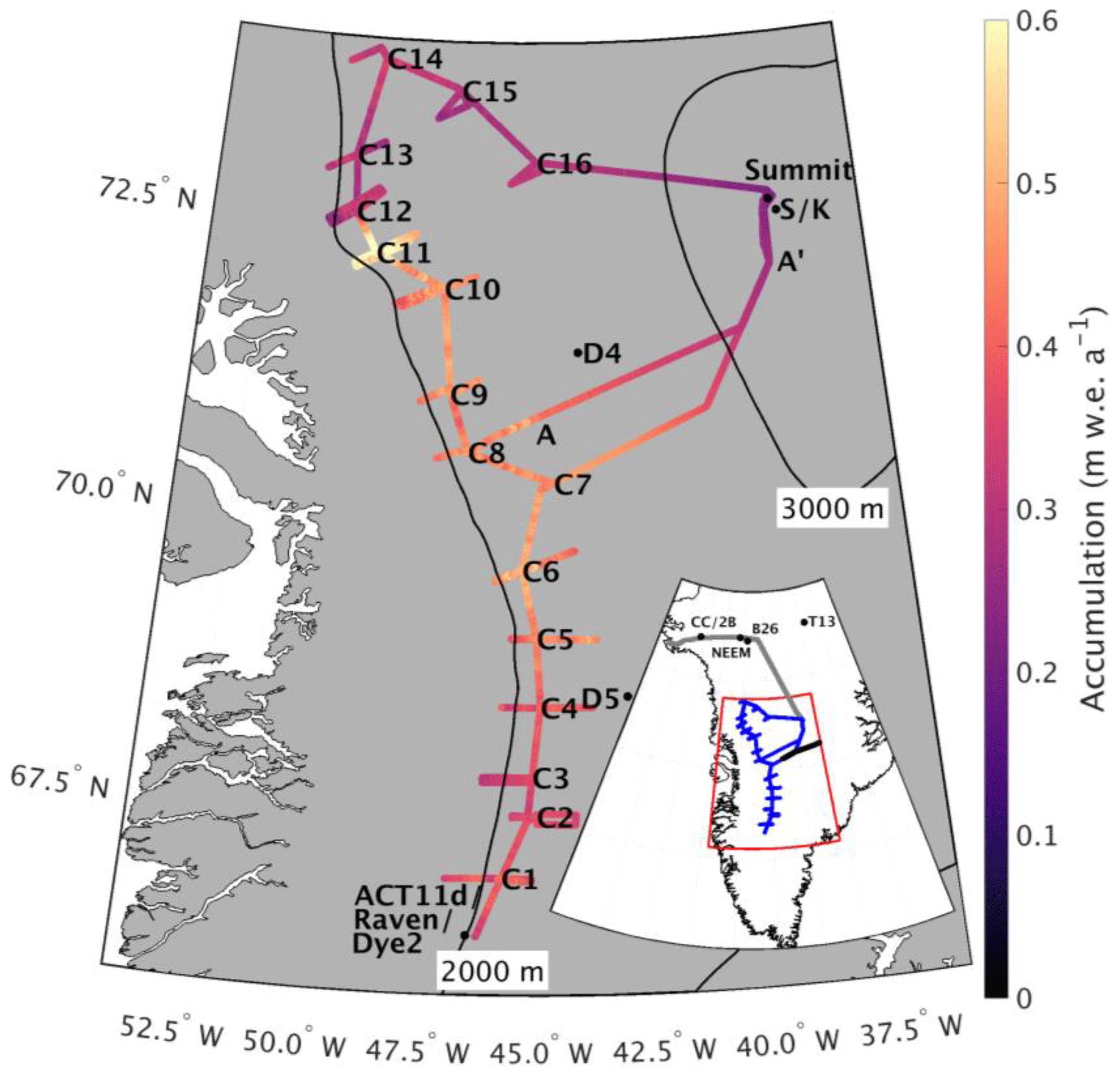
Figure 1Average accumulation rates across the GreenTrACS traverse for the length of each record showing the location of each firn core, ACT11d, D4, D5, Katie (K), Raven–Dye-2, and Sandy (S) ice cores, and Summit Station. Transect A–A′ discussed in Sect. 3.3. Inset shows locations of Camp Century (CC), 2Barrel (2B), NEEM, B26, and TUNU2013 (T13) ice cores, as well as locations of EGIG (black), GrIT (grey), and GreenTrACS (blue) traverses.
2.1 GPS
During the 2016 traverse we collected GPS data using a Trimble NetR8 reference receiver with a Zephyr Geodetic antenna mounted to a Nansen sled ∼5 m in front of the GPR antenna. For each spur and the tail ends of each transect between core sites we performed differential corrections to the GPS data using RTKLIB 2.4.1 and a Trimble NetR8 base station near the core site. Between spurs, when not operating a base station, we post-processed GPS data in precise point positioning mode (Zumberge et al., 1997). Estimated root-mean-square horizontal errors were generally between 13 and 18 cm from standard deviations calculated during stationary periods at the end of spurs. To co-register GPR and GPS data, we used time stamps embedded in the two data streams and locations where we stopped to save GPR files, approximately every 15 km. The time drift in the GPR logger is negligible over these durations.
During the 2017 traverse we used GPS data from a Garmin 19x GPS receiver wired directly to the GPR instrument, which recorded position data at every radar sample with rms values of 3 m. During radar processing we average 75 adjacent traces, corresponding to a distance of ∼20 m, so errors in GPS positioning have a negligible effect on the final dataset.
2.2 Ground-penetrating radar
We develop a spatially continuous record of accumulation rates using GPR profiles collected with Geophysical Survey Systems Inc. (GSSI) SIR-3000 (during 2016) and SIR-30 (during 2017) radar units with a 400 MHz antenna (following Hawley et al., 2014). The antenna was towed on the snow surface in a small plastic sled ∼5 m behind a wooden Nansen sled and ∼15 m behind a snow machine. We recorded 2048 samples (2016) and 4096 samples (2017) per trace over a range window of 800 ns (Fig. 2). The 400 MHz short-pulse radar has a range resolution (ability to resolve distinct features) of 0.35±0.10 m in firn, which is fine enough to resolve internal reflecting horizons (IRHs) that have been shown to represent isochrones (Medley et al., 2013; Rodriguez-Morales et al., 2014; Spikes et al., 2004; Hawley et al., 2014). We recorded 10 traces per second, which at the snowmobile's average travel speed of approximately 2.75 m s−1 results in ∼3.6 traces recorded per meter. Note that this spacing between traces varies with vehicle speed.

Figure 2Radargram showing the top 32 m of the transect along the main 2017 traverse from Core 13 to Core 15. Cores are indicated as red lines down to their final depth, with dates plotted every 5 years at corresponding depths. Traced internal reflecting horizons are shown as isochronous green lines. The depth scale on the vertical axis is calculated from the two-way travel time-to-depth conversion (see Sect. 2.4) for Core 13, although there is no visual difference in depth scale across this radargram.
Depending on signal attenuation within the firn column, IRHs can be traced to a depth of 20–50 m (Fig. 2), providing accumulation records over the past 20–60 years (Fig. 3). For areas with high attenuation (i.e., shallow penetration of the radar signal), such as lower-elevation regions with more refrozen melt layers, we calculate accumulation results for shorter time periods. We are not able to trace as many IRHs to the west of Cores 10–13 compared to the east due to higher signal attenuation (Fig. 3), resulting in slightly different (less than 0.03 m w.e. a−1) average accumulation values on either side of these core locations. Likewise, we experienced an equipment malfunction at the end of the 2016 traverse, reducing the number of observable IRHs from Core 7 to Summit Station (Fig. 3). We have less confidence in calculated accumulation rates throughout this section of the traverse due to this malfunction, although the 2017 Summit to Core 8 interval overlaps nicely with the last 140 km of the problematic 2016 interval, and provides high-quality accumulation measurements for this section near Summit Station.
We reduce the GPR data volume and signal noise by averaging 75 adjacent traces, which has the effect of suppressing random noise by the principle of trace stacking (Yilmaz, 2001). We apply a combination of median trace filtering, residual mean filtering (Gerlitz et al., 1993), and bandpass filtering using a butterworth design (Selesnick and Sidney Burrus, 1998) between 200 and 800 MHz. For data visualization, we apply an automatic gain control (Yilmaz, 2001) to give the interpreter more confidence when picking IRHs.
2.3 Firn core processing and density profiles
The amount of snow mass and the time span between IRHs are necessary to calculate accumulation rates from the GPR profiles. The accumulation rate is a function of the depth–age scale, travel time–depth conversion rate, and the firn density profile. We obtain the depth–age and depth–density scales from each of the shallow firn cores collected along the GreenTrACS traverse, and from density models based on temperature and accumulation rate data.
The 16 firn cores were drilled using an Ice Drilling Program hand auger with a Kyne Sidewinder attachment (see Graeter et al., 2018). We sampled the firn cores for chemical measurements using a continuous ice core melter system with discrete sampling at Dartmouth College (Osterberg et al., 2006). We used an Abakus (Markus Klotz GmbH) laser particle detector to measure microparticle concentrations and size distribution from the continuous ice core meltwater stream, a Dionex model ICS5000 capillary ion chromatograph to measure major ion (Na+, Mg2+, Ca2+, K+, , Cl−, , ) and methanesulfonic acid concentrations, and a Picarro L1102-I and a Los Gatos Research liquid water isotope analyzer to measure oxygen and hydrogen isotope ratios (δ18O, δD; Graeter et al., 2018).
We determined depth–age curves by identifying annual layers based on robust seasonal oscillations in δ18O and the concentrations of major ions, methanesulfonic acid, and dust, consistent with previous ice core studies (Graeter et al., 2018; Mosley-Thompson et al., 2001; Osterberg et al., 2015). We combined the depth–age curves with core density to calculate annual accumulation rates.
We determine depth–age curves for each core by identifying annual layers based on seasonal oscillations in δ18O and the concentrations of major ions and dust, consistent with previous ice core studies in this region (Graeter et al., 2018; Mosley-Thompson et al., 2001; Osterberg et al., 2015). While meltwater percolation smooths the signal of some of these tracers, we can still confidently determine the depth–age curve using nearly unperturbed oscillations in δ18O and dust. We combine the depth–age scales with measured density to calculate annual accumulation rates at the firn core sites.
At each firn core and at the ends of each spur, we measured the density in the top meter of snow using a 1000 cm3 Snowmetrics cutter. To calculate density profiles from the firn cores, we measured the mass, length, and diameter of 0.03–1 m long core segments in the field and again after transporting the cores to the Dartmouth College Ice Core Laboratory. Additionally, we measured melt layer thickness in the laboratory following Graeter et al. (2018). To calculate accumulation rates at Raven–Dye-2, we use density data from a 119.6 m long firn core collected in 1997 (Bales et al., 2009) and a 19.3 m long core collected from the same location in 2015, which did not include accumulation rate data (Vandecrux et al., 2018). For this location we use the most recent density data for the near surface and the older densities for depths below the 2015 core. Likewise, we use a density profile from a 109 m long firn core collected from Summit in 2010 (Mary Albert, personal communication, 2015). We also incorporate density data from measurements along the EGIG traverse at T19, T21, T23, T27, and T31 to improve the density profile between Core 7 and Summit (Morris and Wingham, 2014).
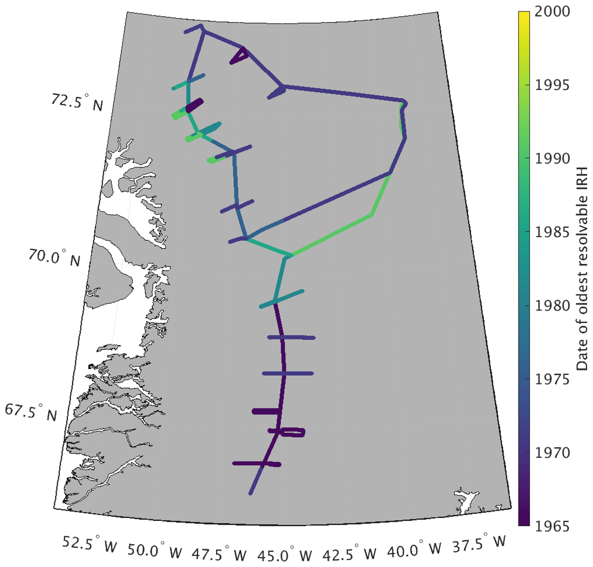
Figure 3Date of oldest resolvable internal reflecting horizon throughout the entire GreenTrACS traverse route. Anomalously young ages from Core 7 to Summit are due to equipment malfunction.
After collecting each firn core, we measured borehole temperature for 24–48 h using a 20 m long thermistor string. We estimate mean annual temperature from the deepest thermistor on the 20 m long thermistor string. These measurements agree with MODIS satellite-derived mean annual surface temperature (Hall et al., 2012) to within ±1 ∘C for each firn core location. The small amount of energy released from refreezing of summertime percolation water has diffused by the time of our measurements, allowing for direct comparison between in situ firn temperature and MODIS clear-sky measurements. For the location of each firn core, we use the depth–density data from that core and calculate a Herron and Langway (1980) depth–density model for depths below the core using our measured mean annual temperature, firn core mean annual accumulation rates, and top-meter snow density. Likewise, we calculate Herron–Langway profiles for the ends of each spur using MODIS satellite-derived mean annual temperature (Hall et al., 2012), MAR-modeled accumulation rates (Burgess et al., 2010), and the measured snow density in the upper meter of each of the spur's snow pits. Finally, we interpolate depth–density profiles both between firn cores and along radar spurs to estimate the depth–density matrix everywhere along our traverse (Fig. 4). Final calculated accumulation rates are insensitive to the input accumulation parameter we use to calculate our Herron–Langway models (Lewis et al., 2017).
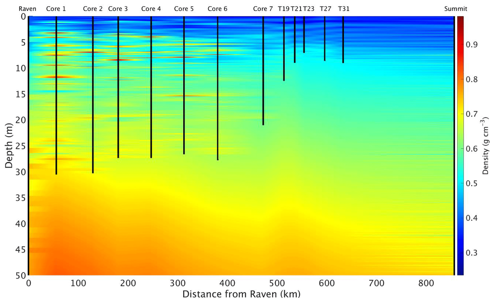
Figure 4Depth–density profile along the main 2016 traverse used for calculation of electromagnetic wave velocity and accumulation rates in this study. Densities are linearly interpolated between the two nearest cores and are modeled using Herron–Langway profiles below the depth of each core. The left and right boundary data come from the Raven–Dye-2 and Summit firn cores, respectively. Ice layers in Cores 1–5 are clearly visible as red lenses, but their extent is, in reality, likely more localized.
As shown in Fig. 4, ice layers within several firn cores are extrapolated laterally along the traverse, although these dense lenses are typically both localized and heterogeneous at these elevations (Brown et al., 2011; Rennermalm et al., 2013). Numerous studies have documented the heterogeneity of firn throughout the percolation zone and the complications of calculating SMB due to ice pipes and lenses (Brown et al., 2011, 2012; de La Peña et al., 2015). Here we attempt to accurately calculate accumulation rates using interpolated firn cores and in situ GPR throughout this complicated region. Our ice lens density interpolation is as accurate as possible between firn cores without additional in situ data, and this estimation does not significantly alter our results, as discussed in Sect. 2.6, since the ice layers represent a small fraction of the total depth to IRHs.
2.4 Travel time to depth conversion
We convert the radar travel time to depth by iteratively multiplying the velocity of the electromagnetic wave by the signal's one-way travel time to each internal reflecting horizon (IRH). The electromagnetic speed of the radar wave, v (m s−1), is calculated from the relative dielectric permittivity, εr (dimensionless), and the speed of light in a vacuum, c (3×10⁸ m s−1), from
In turn, we calculate the relative dielectric permittivity from the density, ρ (g cm−3), of snow and ice at depth, as shown in Fig. 4, for each radar trace at every range bin (following Kovacs et al., 1995) by
We calculate the depth of each subsequent radar sample for each trace in the profile using the radar travel time and velocity profile from Eqs. (1) and (2), following Hawley et al. (2014) and Lewis et al. (2017).
2.5 Internal reflecting horizons
We manually select 10 clear, strong IRHs spaced approximately 5 years apart to consistently trace from Raven–Dye-2 to Summit Station and throughout the 2017 main traverse (Fig. 2). We trace each layer manually by visually identifying strong amplitude peaks throughout the radargram, starting with the 2016 layer and working downwards. We use a spline interpolation between manual picks to trace each layer along large amplitude reflections every ∼500–700 m along the traverse. When a layer appears to bifurcate due to changes in snow accumulation, we continue to trace the layer based on the trajectory of surrounding IRHs. Each horizon is traced throughout the traverse, except in areas where the attenuated signal makes it too difficult to interpret (Fig. 3). We trace layers for each spur starting at the depth of each layer at the corresponding firn core location. Layers below the depth of some firn cores are traced from nearby cores that are deeper or have lower accumulation rates.
We trace layers between cores using a connect-the-dots approach using the depth–age scale at each firn core. After tracing layers from one firn core to the next, we check that layers intersect the core location at the proper depth for the age of our traced IRH. Note that the depths of several layers at Cores 2–16 are located below the bottom depth of those cores. Since these layers are isochronous, they are used to calculate accumulation rates over appropriate time epochs by using dates obtained from intersections with other cores (see Fig. 3).
2.6 Accumulation rate calculations and uncertainty
Finally, we calculate snow accumulation rates using the firn core depth–age scales, measured and interpolated depth–density profiles (Fig. 4), and traced IRHs (Fig. 2). We calculate the water-equivalent accumulation rate (m w.e. a−1) between adjacent IRHs from the depth z (m) and age t (year) of each layer, the average density ρ (kg m−3) between layers, and the density of water ρw (1000 kg m−3):
We correct for layer thinning using a Nye (1963) model. The thinning factor has an average value of 0.9993±0.0003 and is multiplied by the accumulation rate for each radar trace. For each radar trace, the thinning factor, λ(z), is calculated from the average accumulation rate (m w.e. a−1) of each epoch, average age of the epoch a (year), and water-equivalent thickness of the GrIS H (m), from Morlighem et al. (2014):
Accumulation uncertainty can arise from independent errors in tracing IRHs, errors from incorrectly dating firn cores, and/or errors in the densities used for converting from separation distance to water-equivalent accumulation rates. To reduce tracing errors, we retraced each IRH along the two main traverse paths four times apiece. Close inspection of the IRHs reveals that the peaks defining IRHs are within ±2 radar samples (within at most ±0.12 m), and incorrectly jumping to the next IRH would result in an error of at most ±10 samples (within ±0.55 m). We chose an epoch between IRHs of 5.0 years from the firn core chemistry depth–age scales, which corresponds to a maximum tracing error of m a−1 for each epoch, or a maximum error of ±0.061 m w.e. a−1 given an average firn density of 0.55 g cm3 across this dataset.
We perform a leave-one-out cross validation to calculate accumulation errors at locations where we do not have firn core density profiles. Here we choose one of the 16 firn cores, in addition to the Raven–Dye-2 and Summit cores, to omit from our density interpolation (Fig. 4), so that we interpolate density profiles between adjacent firn cores and a Herron–Langway profile at the missing core location. We find maximum single-epoch errors of 0.079 m w.e. a−1 and maximum rms (1971–2016) errors of 0.046 m w.e. a−1 (Fig. 5) at the location of missing cores. These differences are approximately twice as large at Cores 1–6 than Cores 7–16 due to larger differences between measured and interpolated density profiles, likely a result of meltwater percolation and ice lenses (Graeter et al., 2018).
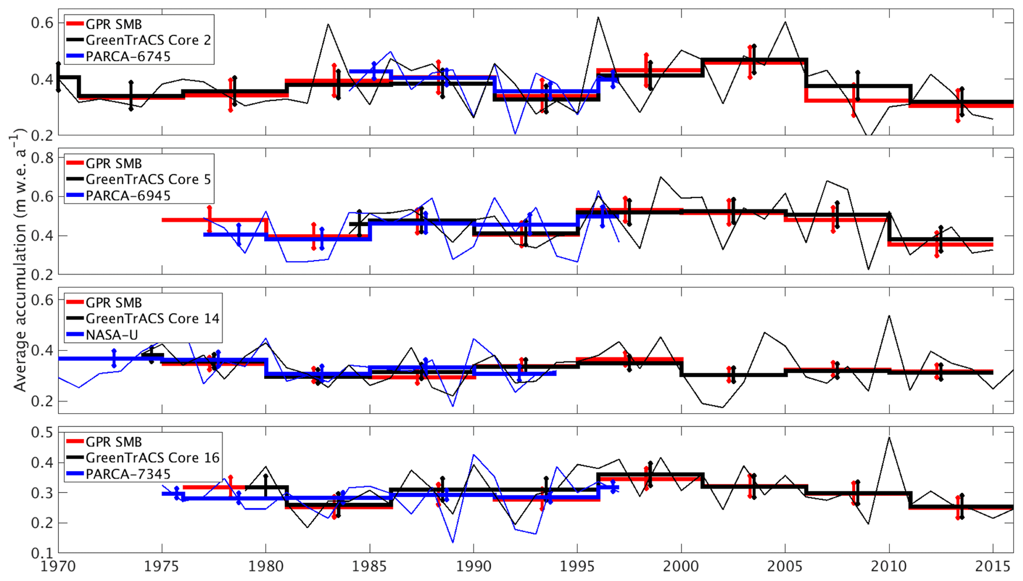
Figure 5Accumulation rates from GPR and collected firn cores (this study) compared with cores from the PARCA Campaign. Thin lines represent annual PARCA (blue) and GreenTrACS (black) firn core accumulation rates, while thick lines are 5-year averages over corresponding GPR epochs. Error bars represent one standard deviation over each epoch. GPR and PARCA accumulation rate averages and decadal trends are statistically indistinguishable.
Similarly, we perform a leave-one-out validation by omitting a firn core density profile location entirely and interpolating density profiles over a larger distance (e.g., between Core 1 and Core 3). In this case we find maximum single-epoch errors of 0.057 m w.e. a−1 and maximum rms (1971–2016) errors of 0.033 m w.e. a−1. Throughout this study, we use our measured density profiles to calculate accumulation rates at core locations, rather than rely on Herron–Langway density models that would result in larger uncertainties.
We conservatively take our accumulation error from missing density measurements to be 0.079 m w.e. a−1. This error highlights the importance of our firn core spacing between 40 and 100 km along the traverse and confirms that the accuracy of future remotely sensed radar accumulation (e.g., IceBridge snow and accumulation radars) estimates depends on precise field-based in situ density profiles for accurate accumulation history in the percolation zone. Overly et al. (2016) calculated accumulation rates in the dry snow zone using Herron–Langway profiles within 3.5 % of accumulation rates calculated using neutron-probe density profiles. However, here we show that in situ measurements, or accurate meltwater percolation modeling (Meyer and Hewitt, 2017), are required to correctly calculate SMB in the percolation zone.
We assume uncertainty in dating the firn cores from annual variations in chemistry to be ±0.5 years (Buchardt et al., 2012). At the lowest accumulation rate locations, the smallest distance between layers is 0.15 m w.e. over an epoch of 4.91 years. This gives an uncertainty in accumulation rates due to dating of at most m w.e. a−1. The error associated with measuring in situ firn density has been estimated to be 1.4 % (Karlöf et al., 2005). However, following Hawley et al. (2014) and Lewis et al. (2017), we conservatively assume that our measurements have a density measurement error of up to twice as large, corresponding to a maximum accumulation error of ±0.014 m w.e. a−1.
We calculate the total uncertainty from formal error propagation (following Bevington and Robinson, 1992) from the average accumulation rate m w.e. a−1, average thickness between IRHs Δh=3.56 m, uncertainty in tracing ρ=0.550 g cm3, uncertainty in density measurements δρ, average time period between IRHs Δt, and uncertainty in core dating δt. We find the total accumulation rate uncertainty for each epoch to be 0.071 m w.e. a−1 from Eq. (5).
Due to the random and non-systematic nature of these errors, we can assume that they are unlikely to contribute to a regional or temporal accumulation rate bias. To calculate uncertainty for accumulation rates averaged over multiple epochs (σn−epochs) we divide our uncertainty σepochs by the square root of the number of traced layers (n) at that location.
2.7 Model comparison
We compare our GreenTrACS accumulation results with annual outputs from Box et al. (2013; hereafter “Box13”; 1840–1999), the Fifth Generation Mesoscale Model (Polar MM5; 1958–2008; Burgess et al., 2010), MAR (1948–2015; Fettweis et al., 2016), and the Regional Atmospheric Climate Model (RACMO2; 1958–2015; Noël et al., 2018) over common time periods. Grid cell sizes for these model outputs are 5, 3, 5, and 1 km, respectively. For each radar trace we calculate statistically significant differences (at α=0.05) using a two-sample t test with the GreenTrACS accumulation records for each epoch and RCM accumulation rates for each common year. Additionally, we compare our GreenTrACS accumulation rates with an accumulation map kriged from 295 firn cores and 20 coastal weather stations (Bales et al., 2009; hereafter “Bales09”). We perform the same two-sample t test with the reported Bales09 uncertainty of 0.092 m w.e. a−1 (Bales et al., 2009).
2.8 Accumulation trends
To investigate recent changes in GrIS accumulation rates, we calculate trends in accumulation rates across our GPR and GreenTrACS firn core dataset. We fit a linear model to the accumulation rate time series for each radar trace and analyze the trend for both slope and statistical significance. Likewise, we calculate trends and their statistical significance for total precipitation (snowfall + rainfall) for MAR and RACMO2 grid cells from 1996 through the end of both models' temporal coverage. We can compare these results with our accumulation trends since precipitation and accumulation rates are nearly identical above the equilibrium line altitude, due to zero runoff and negligible sublimation within the percolation zone.
2.9 Storm track changes
To investigate the potential role of changing storm tracks in precipitation changes over the western GrIS, we utilize the updated Serreze (2009) storm track database. This database contains 6 h interval positions of extratropical cyclone storm centers on a 2.5∘ grid. These centers are defined when a grid point sea level pressure is surrounded by grid points at least 1 hPa higher than the central point (Serreze, 2009). We calculate the total number of days on which a storm center is located within our region of interest for each season. To determine statistical significance, we run a two-sample t test on the number of storms in our region of interest between 1958 and 1996 compared with 1996–2016.
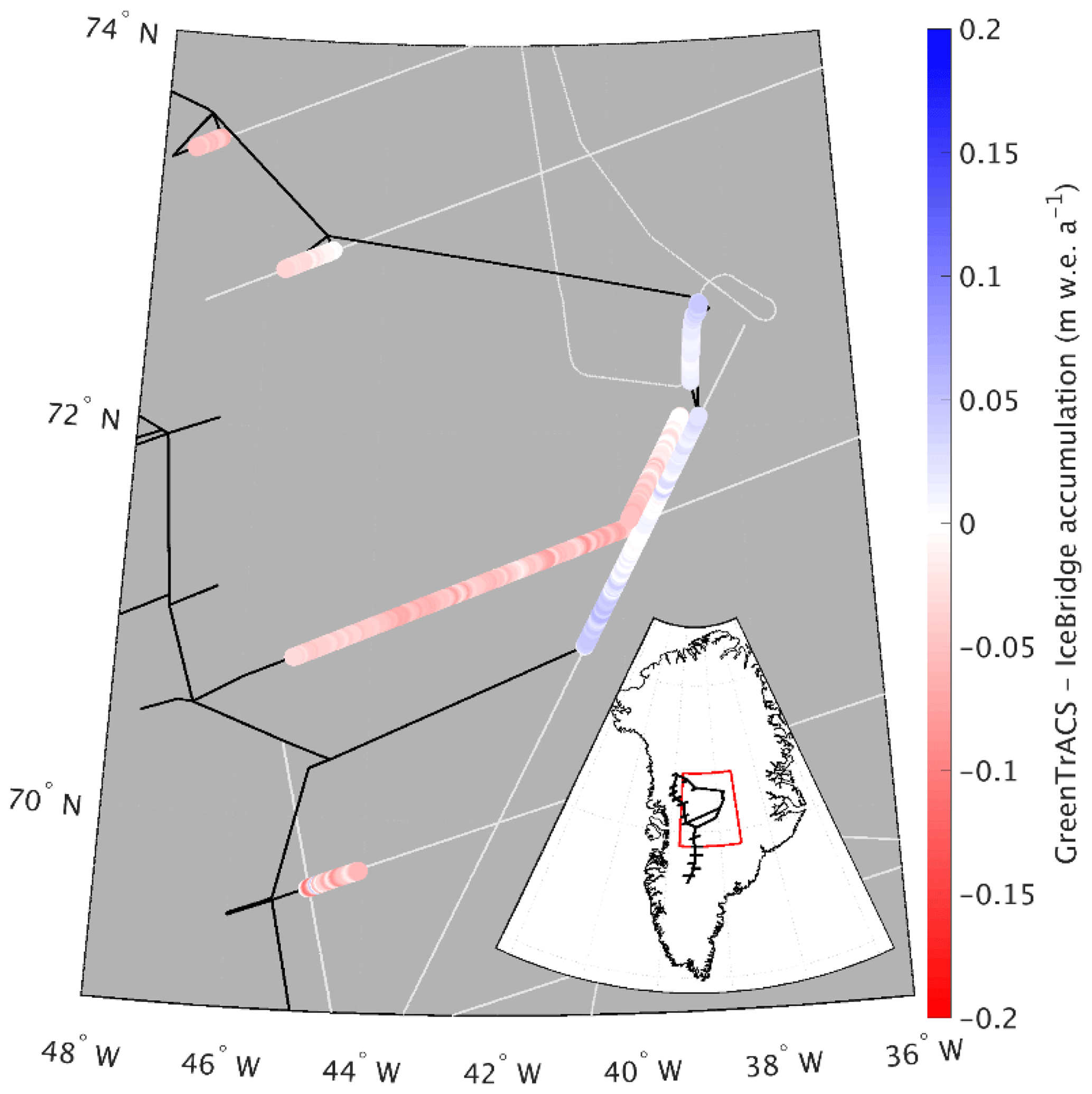
Figure 6Difference between averaged (1966–2016) GreenTrACS accumulation and average (1962–2014) IceBridge Accumulation Radar rates from Lewis et al. (2017) across all 562.5 km of overlap. Spatially overlapping section of 2016 and 2017 traverses displayed as adjacent tracks. Also showing extent of GreenTrACS traverse (black) and IceBridge accumulation radar (grey). Inset shows map location with respect to GreenTrACS traverse (black).
3.1 Firn core and GPR accumulation records
Figure 1 displays the mean accumulation rates at each location along the traverse route, with higher accumulation rates along the main traverse and lower accumulation rates at higher elevations of the ice sheet interior, broadly consistent with previously published accumulation rate compilations (e.g., Bales et al., 2009) and RCM output (Box et al., 2013; Burgess et al., 2010; Fettweis et al., 2016; Noël et al., 2018). We analyze localized differences between GPR-derived accumulation rates and these RCMs in Sect. 3.3. There is an especially high accumulation rate zone near Core 11 (0.685 m w.e. a−1), nearly double the accumulation rate at Core 10 (0.453 m w.e. a−1) and Core 12 (0.327 m w.e. a−1), respectively situated only 43 km northwest and 73 km southwest of Core 11. In the GPR data, the number of traceable IRHs is highest towards the interior of the ice sheet and lowest in warmer areas towards the coast and in the south, where refrozen percolated meltwater from enhanced surface melt attenuates the radar signal and reduces the number of observable IRHs (Brown et al., 2011; Fig. 3).

Figure 7Average GreenTrACS GPR accumulation rates (black) compared with (a) IceBridge accumulation radar, (b) Bales09 kriged ice core map, (c) MAR, (d) RACMO2, (e) Box13, and (f) Polar MM5. GPR measurements are statistically indistinguishable from each of the other measurements along this 285 km transect in the dry snow zone (A–A′ in Fig. 1).
3.2 Validation with past measurements
We validate our accumulation record with published core records from the PARCA campaign and accumulation data from the NASA IceBridge program. The locations of GreenTrACS core sites 2, 5, 9, 10, 11, 14, 15, and 16 were chosen to reoccupy PARCA core locations 6745, 6945, 7147, 7247, 7249, NASA-U, 7347, and 7345, respectively. These GreenTrACS cores overlap with the accumulation history of each PARCA core and extend the record from 1997/1998 to 2016/2017. Annual and epoch-averaged accumulation rates derived from GreenTrACS firn cores are within uncertainty ranges of those determined from corresponding PARCA cores during the period of overlap. Averaging accumulation rates over 5-year epochs reduces noise in year-to-year accumulation variability. Figure 5 compares the accumulation records from PARCA sites 6745, 6945, 7345, and NASA-U to their corresponding GreenTrACS cores, demonstrating that each pair of cores has similar long-term mean accumulation rates and nearly identical decadal variability. Thus, we have confidence in firn-core-derived accumulation rates that are used in subsequent GPR calculations of accumulation rates throughout the GreenTrACS traverse.
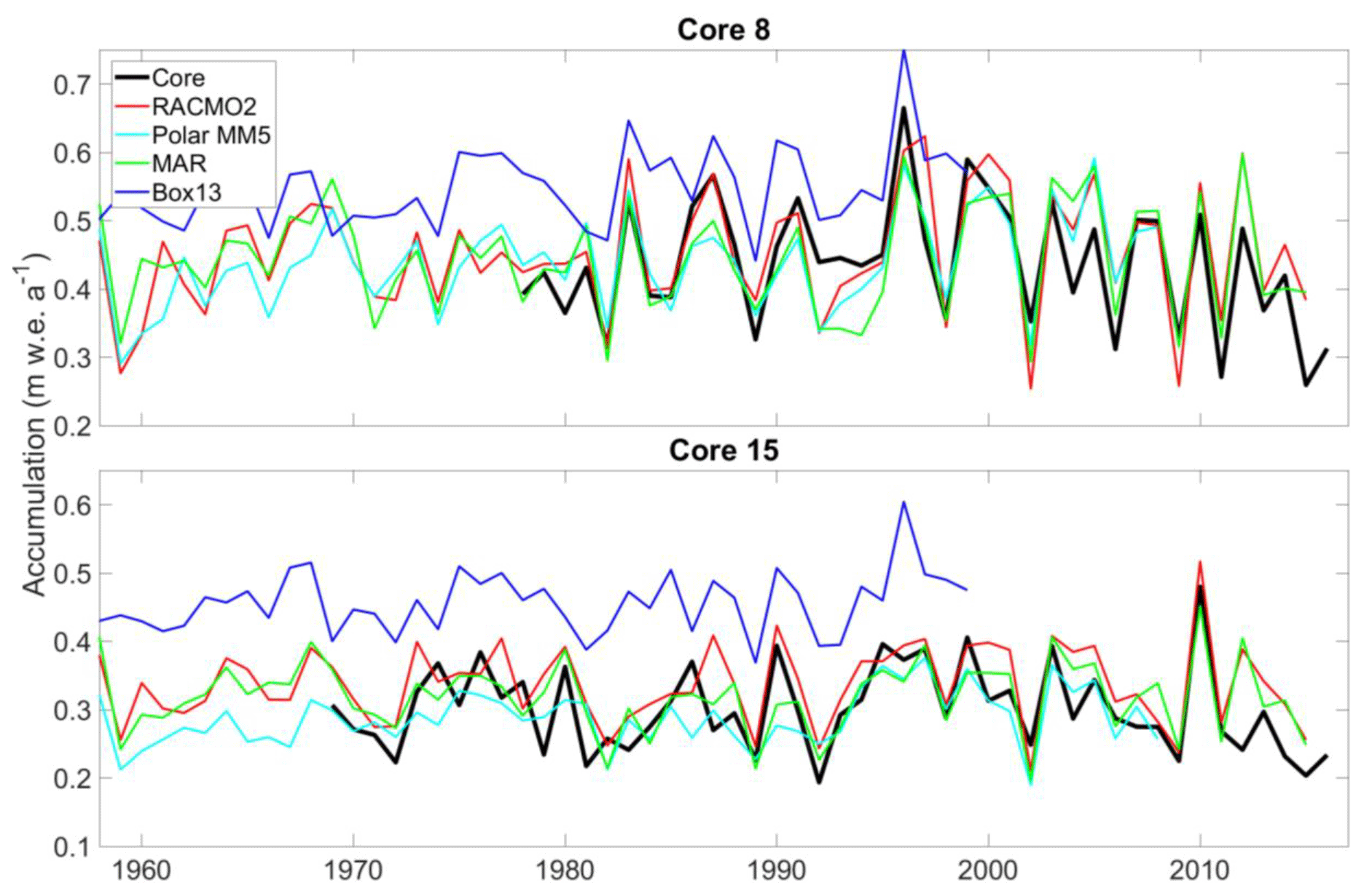
Figure 8Accumulation record at GreenTrACS Core 8 and Core 15 (black) compared with RCM output from RACMO2 (red), Polar MM5 (cyan), MAR (green), and Box13 (blue). We find statistically significant Pearson correlation coefficients between GreenTrACS and RCM accumulation rates for these cores (see Table 2).
Average (1966–2016) GPR accumulation rates are statistically indistinguishable from average (1962–2014) IceBridge Accumulation Radar measurements analyzed by Lewis et al. (2017), with an rms difference of 0.039±0.033 m w.e. a−1 (6.0±9.6 %) along a total of 562.5 km of overlap (Fig. 6). The disagreement is largest at lower elevations, where Herron–Langway profiles used in Lewis et al. (2017) differ the most from GreenTrACS firn core density profiles in the upper 30 m of firn, demonstrating the importance of field observations for calibration and validation. The close agreement at higher elevations is illustrated in Fig. 7a, where our GreenTrACS accumulation measurements are statistically indistinguishable from the IceBridge radar-derived accumulation rates (Lewis et al., 2017) along the 285 km A–A′ transect in Fig. 1. Notice that the uncertainty in GreenTrACS accumulation rates progressively decreases higher in the percolation zone and into the dry snow zone (towards the right in Fig. 7) along this transect as density becomes less heterogeneous from fewer melt layers (Graeter et al., 2018) and IRHs become easier to trace.
Similarly, our 2011–2016 accumulation rates are statistically indistinguishable from average 2009–2012 IceBridge snow radar measurements analyzed by Koenig et al. (2016), with an rms difference of 0.049±0.096 m w.e. a−1 (14.0±27.7 %) along a total of 69.7 km of overlap (not shown). Koenig et al. (2016) use a different radar system on an airborne platform and are able to calculate annual accumulation rates at elevations below 2000 m a.s.l.; however the GreenTrACS accumulation record covers a longer temporal duration than the data from that study.
3.3 Comparison to modeled accumulation
We assess differences between RCM accumulation output and GreenTrACS accumulation records at each firn core site, two of which are shown in Fig. 8. In general, year-to-year correlations between GreenTrACS firn core accumulation records and RCM output for the corresponding grid cell are strong, positive, and statistically significant (Table 2). On average, GreenTrACS firn cores' correlation coefficient with MAR output is 0.718, with PolarMM5 is 0.701, with Box13 is 0.607, and with RACMO2 is 0.763. Every correlation is statistically significant at p<0.05 except for Cores 7 and 11 with Box13. We do not report a correlation coefficient for Core 11 and Box13 because they only share two common years. Temporal correlation coefficients remain high even at locations with large magnitude differences between RCM output and firn core accumulation rates. For example, the Box13 model overestimates accumulation rates at Core 15 by 0.15±0.05 m w.e. a−1, on average, but the model output has a correlation coefficient of 0.48 with Core 15 (Table 2) and matches years of high accumulation rates (e.g., 1987, 1990, and 1996) and low accumulation rates (e.g., 1981, 1989, 1992).
Table 1Difference between accumulation rates at each GreenTrACS core site calculated using Herron–Langway profiles and firn core density information.
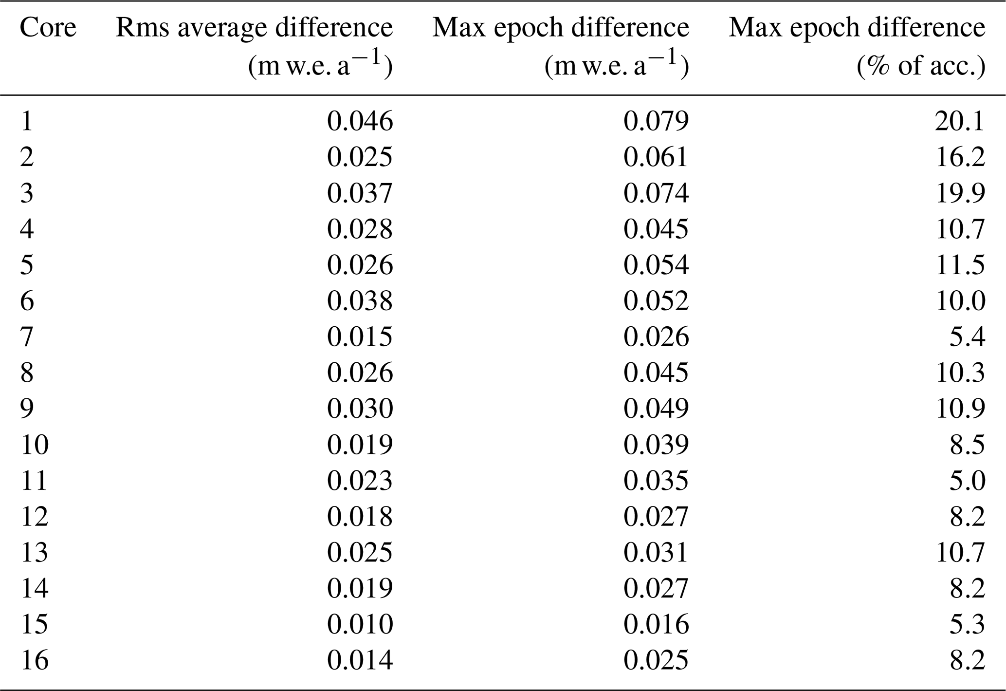
Table 2Pearson correlation coefficients between accumulation rate time series from firn cores and co-located RCM output over their common time period*.
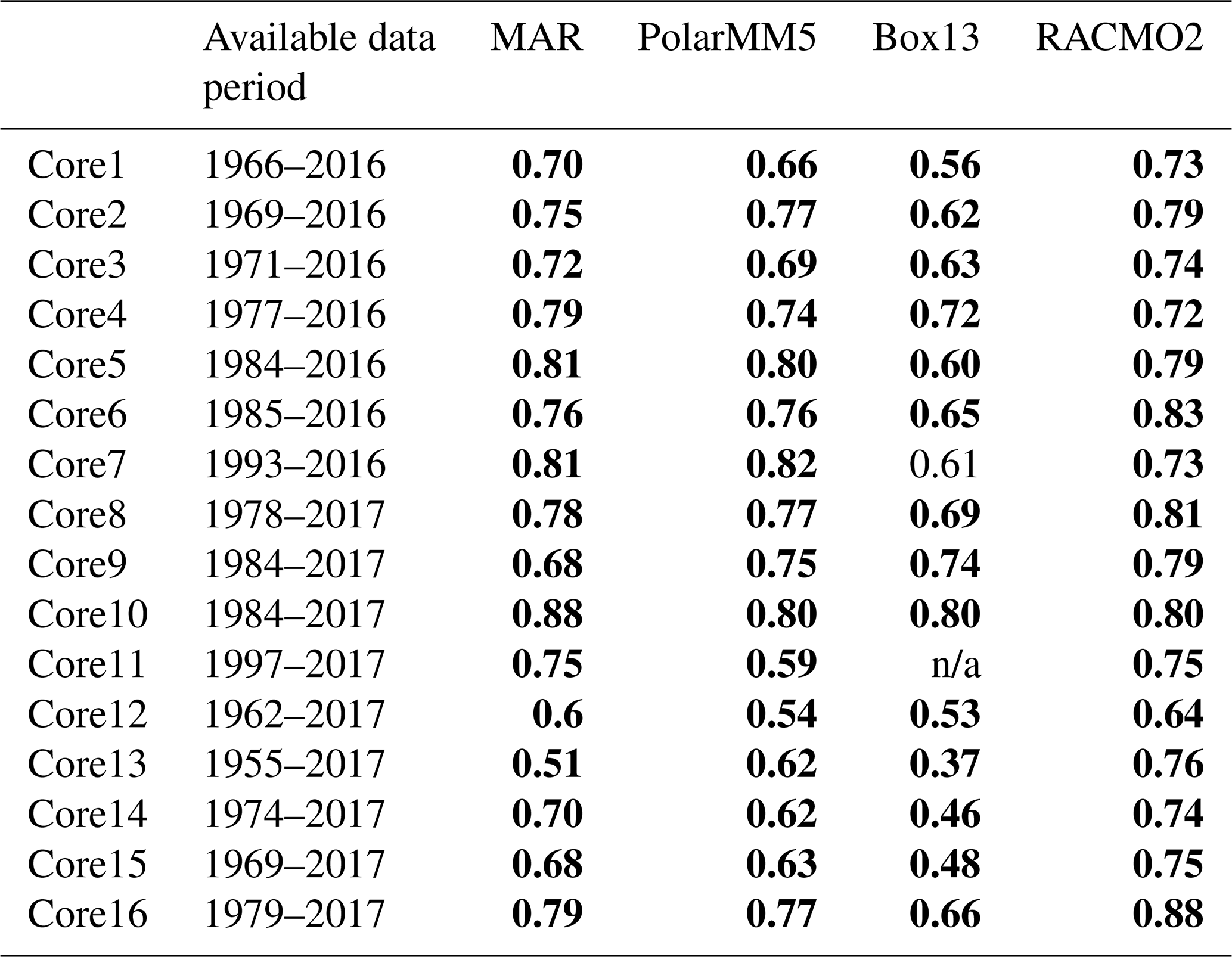
* Statistically significant correlations (p<0.05) are bold. n/a – not applicable.
We also assess spatial differences between GreenTrACS accumulation rates and mean RCM accumulation rates averaged over several decades (Table 2). Figure 9 shows that differences between GreenTrACS accumulation rates and RCM output increase in magnitude, become more spatially heterogeneous, and vary by model at lower elevations of the ice sheet where topographic variations are larger and surface melt increases. Averaged over all 4436 km of the traverse, the rms difference (±1σ) between each model and GreenTrACS accumulation rates over corresponding data periods (Table 2) is 0.068±0.065 (MAR), 0.056±0.055 (RACMO2), 0.082±0.070 (Box13), 0.048±0.045 (Polar MM5), and 0.048±0.045 m w.e. a−1 (Bales09). We find that RCM differences from GreenTrACS accumulation rates are small in the dry snow zone (Fig. 9). For example, Fig. 7 shows that average GreenTrACS accumulation measurements from 1966 to 2016 along the A–A′ transect in Fig. 1 are statistically indistinguishable from those derived from the Bales09 kriged ice core map (Fig. 7b), MAR (1966–2015; Fig. 7c), RACMO2 (1966–2013; Fig. 7d), Box13 (1966–1999; Fig. 7e), and Polar MM5 (1966–2008; Fig. 7f).
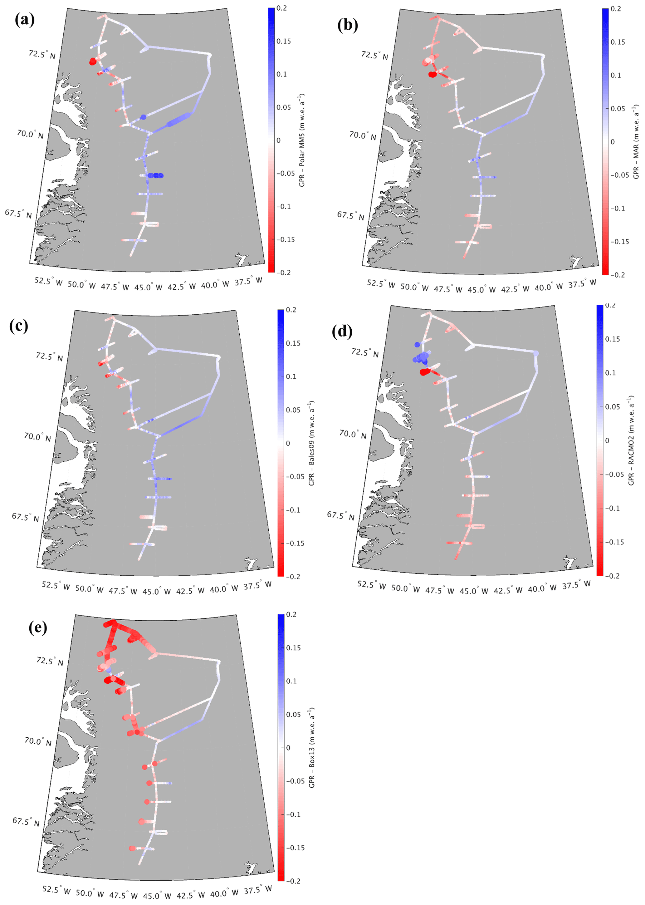
Figure 9Differences between GreenTrACS accumulation rates and (a) Polar MM5, (b) MAR, (c) Bales09, (d) RACMO2, and (e) Box13 accumulation rates averaged over the corresponding time periods. Large dots show statistically significant differences from GreenTrACS accumulation rates.
However, the high spatial resolution of our dataset shows significant accumulation variability not captured in model output (Fig. 9). For example, Polar MM5 and MAR both underestimate accumulation rates between Core 4 and Summit, while overestimating accumulation rates to the west of Cores 10–12. Likewise, RACMO2 overestimates accumulation rates between Raven–Dye-2 and Core 5 by 0.03 to 0.08 m w.e. a−1 and shows statistically significant differences east of Cores 11 and 12. Bales09 accurately calculates accumulation rates along most of the 2016 traverse, but overestimates accumulation rates west of Cores 11 and 12 by 0.135±0.041 m w.e. a−1. Finally, Box13 overestimates accumulation rates along many of the western spurs and has statistically significant overestimations of 0.1 to 0.4 m w.e. a−1 between Cores 10 and 16. Box13 overestimates 67.8 % of the data in the Core 10–16 region by at least 0.1 m w.e. a−1 and 6.6 % of that data by at least 0.2 m w.e. a−1.
Our study is almost entirely contained within drainage basin E from Vernon et al. (2013), who note that basin E is the only major Greenland drainage basin with no statistically significant differences in SMB between the four RCMs. However, differences of 0.1 to 0.4 m w.e. a−1 exist when we look at a local (sub-drainage-basin) scale for each model. All four of the RCMs overestimate accumulation rates along the western spur of Core 11 and they all underestimate accumulation rates along the eastern spur of Core 5 (Fig. 9).
In summary, the RCMs do an excellent job of calculating accumulation rates averaged over this drainage basin, with rms values between 0.048 and 0.082 m w.e. a−1, but there are larger differences of 0.1 to 0.4 m w.e. a−1 between model and GPR accumulation rates on local scales. Differences between GreenTrACS and RCM accumulation rates are largest in areas concurrent with the fewest, shortest, and/or most outdated in situ measurements. For example, the GPR vs. model differences near Cores 11, 12, and 13 are relatively large for all RCMs, despite Core 11 being co-located with PARCA 7249. However, the PARCA cores were collected over 20 years ago, and Core 11 only spanned 7 years because of the high accumulation rate at that site. This highlights the importance of collecting updated field-based measurements to calibrate remotely sensed data and RCM output.
3.4 Accumulation temporal trends
In most locations, there are no statistically significant trends in the GreenTrACS accumulation record from 1966 through the mid-1990s. However, a change-point analysis (Lavielle, 2005) reveals that accumulation rates in the western GrIS percolation zone changed significantly after the 1995–1996 accumulation year. Since 1996, our record indicates a statistically significant average accumulation rate decrease of 0.009±0.005 m w.e. a−2, or 2.4±1.5 % a−1, from 1996 to 2017. Although we observe fewer statistically significant accumulation trends when we expand this analysis to include the entire temporal duration for each firn core, the sign of the trend at each core site does not change.
In Fig. 10, we compare the negative accumulation trend in the GreenTrACS record (1996–2016) to best-fit linear trends in total precipitation (rain + snowfall) across the ice sheet in MAR and RACMO2 simulations over the 1996–2015 and 1996–2013 periods, respectively. Also shown in Fig. 10 are 1996–2016 accumulation trends for all 16 GreenTrACS firn cores (squares), accumulation trends from ACT10A (1996–2010), ACT10B (1996–2010), ACT10C (1996–2010), D4 (1991–2002), D5 (1991–2002), Katie (1991–2002), Sandy (1991–2002), and Summit 2010 (1991–2010) ice and firn cores (stars on ice sheet), and precipitation trends from coastal weather stations (Mernild et al., 2014; stars on coast). Statistically significant trends (p<0.05) in core data are indicated by black dots, while statistically significant trends in the MAR and RACMO2 output are stippled in black.

Figure 10Best-fit linear trends for each grid cell showing magnitude (left) and percent (right) changes in total precipitation for (a, b) MAR (1996–2015) and (c, d) RACMO2 (1996–2013). Statistically significant RCM grid cell trends are stippled black. Also shown are accumulation trends for GreenTrACS firn cores (squares), ACT10A, ACT10B, ACT10C, D4, D5, Katie, Sandy, Summit 2010, and Raven–Dye-2 cores (stars on ice sheet) and precipitation trends from Mernild et al. (2014; stars on coast) with statistically significant trends indicated by black dots.
We find strong agreement between the accumulation rate decrease in the GreenTrACS record and widespread precipitation decreases in the RCMs over the study area (Fig. 10). On average, the RCMs have a more negative precipitation trend than the GreenTrACS record by 0.003±0.005 m w.e. a−2 (0.3±0.77 %) for MAR and 0.002±0.005 m w.e. a−2 (0.45±1.22 %) for RACMO2. Vernon et al. (2013) show a melt-driven decrease in SMB across this drainage basin of 31.1 % (ECMWFd), 61.6 % (RACMO2), 76.5 % (MAR), and 33.5 % (Polar MM5) for the 1996–2008 period. The negative precipitation trends of 2.4±1.5 % a−1 (Fig. 10d) indicate a total of 2539 fewer gigatons of precipitation and a total of 5159 additional gigatons of melt (not shown) over 1996–2013 across the GrIS. Thus, our analysis suggests that a significant decline in snow accumulation rates contributes to declining SMB throughout the western GrIS over recent decades, in addition to increasing surface melt from rising temperatures (van den Broeke et al., 2009, 2016).
3.5 Effects of melt on accumulation trends
Increased melt throughout the 1996–2016 period is a confounding variable when analyzing trends in accumulation rates. With increased melt over the past several decades in this region, meltwater percolates down through several years of firn (Benson, 1962; Graeter et al., 2018; Harper et al., 2012; Wong et al., 2013). This movement of mass into lower years can artificially increase the mass balance at depth and lower the mass balance during the most recent years, which have not experienced as much meltwater percolation from more recent annual layers. Therefore, it is necessary to evaluate the degree to which the recent accumulation rate decrease in the GreenTrACS record is biased by the recent increase in surface melt and percolation.
On average, we find larger negative accumulation trends ( to m w.e. a−2) at the lower-latitude cores that experience more melt, supporting the hypothesis that meltwater percolation and refreezing are enhancing the negative accumulation trend. However, several other lines of evidence support a negative accumulation trend in the study area since 1996. First, we find statistically significant negative accumulation trends at Cores 10, 11, 12, 13, 15, and 16, each of which experience <1.6 cm a−1 of meltwater percolation on average. Additionally, we have confidence that GreenTrACS accumulation trends reported here are not artifacts of meltwater percolation because both MAR and RACMO2 have similar trends in precipitation (Fig. 10). Finally, we evaluate the maximum effect meltwater percolation could have on GreenTrACS accumulation trends over 1996–2016. The largest measured melt layer from our 16 ice cores occurred during 2003–2004 in Core 1 and contains 0.364 m of ice, equivalent to 0.333 m w.e. (Graeter et al., 2018). We add this percolation to 9 years' of accumulation rates using a sine wave (percolation magnitude 0, 0.5, 1, 0.5, 0, −0.5, −1, −0.5, 0), square wave (0, 0, 0, 1, 1, 1, 0, 0, 0), and triangle wave (0, 0.25, 0.5, 0.75, 1, 0.75, 0.5, 0.25, 0) weighted kernel, before recomputing hypothetical accumulation trends over the same time period with additional meltwater percolation. Regardless of the wave-type choice, recalculated trends remain within a factor of 2 of the original SMB trends and do not change sign with additional percolation.
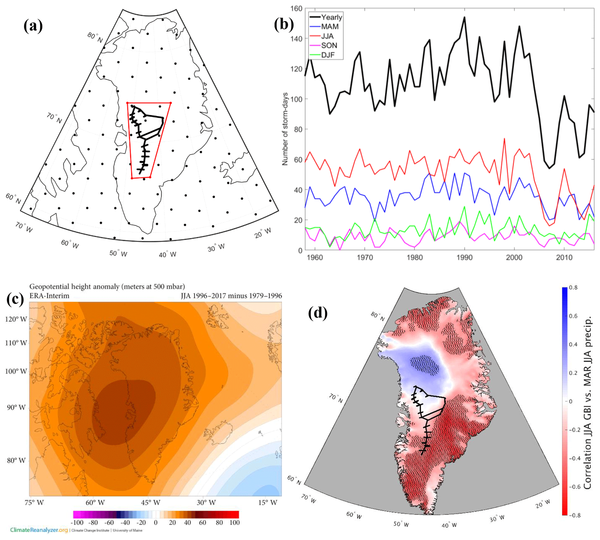
Figure 11(a) Serreze (2009) gridded storm track dataset showing location of GreenTrACS traverse and inquiry box. (b) Total number of storm days within inquiry box for annual and seasonal periods. Horizontal black lines show a decrease in 1958–1996 to 1996–2016 average number of storm days within this region. (c) the 500 mbar geopotential height change over Greenland showing 1996–2016 minus 1979–1996 for the summer season. Image obtained using Climate Reanalyzer (http://cci-reanalyzer.org, last access: 1 February 2019), Climate Change Institute, University of Maine, United States. (d) Correlation between June–August Greenland Blocking Index and MAR June–August precipitation. Statistically significant RCM grid cell correlations are stippled black. GreenTrACS traverse is shown in black.
3.6 Atmospheric circulation drivers of the recent accumulation decline
Our analysis indicates that snow accumulation rates have been declining in western Greenland since 1996, despite significant warming and resulting increases in saturation vapor pressure from the Clausius–Clapeyron relationship. Instead, precipitation decreases over western Greenland likely result from changes in atmospheric and/or oceanic circulation. Mernild et al. (2014) and Auger et al. (2017) found that the positive phase of the Atlantic Multidecadal Oscillation (AMO) is associated with a precipitation increase over interior and southwestern Greenland based on ice core records and the Japanese Meteorological Agency 55 Year Reanalysis (JRA-55; Kobayashi et al., 2015), respectively. In direct contrast with these findings, the decline in western Greenland accumulation rates documented in the GreenTrACS record began in the mid-1990s, contemporaneous with a switch to the AMO positive phase.
We hypothesize that the differences between our results and those of Auger et al. (2017) and Mernild et al. (2014) stem from different causes. Auger et al. (2017) validated the reanalysis data by demonstrating that JRA-55 precipitation at Nuuk, Greenland, is significantly correlated with Nuuk station data from 1958 to 2013. Furthermore, coastal precipitation in western Greenland is strongly and significantly (p<0.05) correlated with precipitation over the interior western GrIS in the JRA-55 dataset (not shown). However, Mernild et al. (2014) found that coastal Greenland precipitation is anti-correlated with ice core accumulation records from the interior GrIS from 1900 to 2000. This suggests that JRA-55 precipitation data, which are not constrained by ice core accumulation records, should be interpreted with caution over the interior GrIS. Mernild et al. (2014) concluded that positive AMO conditions favor higher precipitation over the interior GrIS based on the previous positive AMO phase (1920s to mid-1960s), contrasting with lower accumulation rates during the negative AMO phases (mid-1960s to mid-1990s and prior to the 1920s). However, Mernild et al. (2014) state that the ice core composite record in their analysis may be biased from 1995 to 2000, and they do not analyze precipitation trends after 2000. Thus, the decline in western GrIS accumulation rates documented in the GreenTrACS cores during the latest positive AMO phase from 1996 to 2017 was not captured in the Mernild et al. (2014) analysis. Our results suggest that factors other than the AMO are behind the decline in western GrIS accumulation rates since 1996.
We find that the decrease in accumulation rates over the western GrIS is associated with a significant decrease in the number of storm days since 1996. The GreenTrACS region experienced an average of 115.8±15.3 storm days per year over 1958–1996 and 96.2±27.3 storm days per year over 1996–2016. A two-sample t test indicates that this 17 % decline in storm days is statistically significant (p<0.001). The largest decrease in storm days (25 %) over the GreenTrACS region occurred during summer, with 56.4±6.1 storm days per summer from 1958 to 1996 and 42.3±17.4 storm days per summer from 1996 to 2016 (p<0.0001; Fig. 11b). We also find an increase in the number of storm days in the northwestern GrIS near Thule (not shown).
The decline in summer storm days indicates a relationship with well-documented stronger summer blocking over Greenland over the past 2 decades (Hanna et al., 2013; McLeod and Mote, 2016), with a positive Greenland Blocking Index (GBI) during 17 out of 21 summers between 1996 and 2016 (Hanna et al., 2016). The June–August GBI had a statistically significant positive trend of 1.87 (unitless; normalized to 1951–2000) from 1991 to 2015 (Hanna et al., 2016). The summertime 500 mbar geopotential height increased 50–70 m over the 1996–2016 period compared with the 1979–1996 baseline (Fig. 11c), indicating stronger blocking that we suggest likely reduced precipitation over the central GrIS by deflecting storms poleward from the Greenland interior. This is consistent with an observed 0.9±0.3 % a−1 decrease in JJA cloud cover over Greenland from 1995 to 2009, with the largest decreases in the GreenTrACS region (Hofer et al., 2017). Furthermore, we find a strong negative correlation between ERA-Interim 1979–2015 June–August (JJA) GBI and JJA precipitation in both MAR (Fig. 11d) and RACMO2 (not shown) across the central and southern GrIS. These results suggest that the blocking-induced accumulation rate decline observed in the GreenTrACS region is representative of a broader pattern over the GrIS, with the exception of northwest Greenland where poleward blocking has increased storm days (not shown) and accumulation rates (Fig. 11d).
The effect of summertime Greenland blocking has previously been discussed primarily in the context of increasing surface melt (Hanna et al., 2013, 2018; Ballinger et al., 2017; Hofer et al., 2017), while the effect of blocking on precipitation has received less attention (Hanna et al., 2013; McLeod and Mote, 2016). Our results highlight that stronger summer blocking reduces GrIS SMB through both an increase in surface melting and a decrease in accumulation rates. Stronger summer blocking has been tied to an observed increase in surface melt since 1996 across the western GrIS percolation zone (Graeter et al., 2018), and to the July 2012 melt event, during which 98.6 % of the GrIS experienced melt (Nghiem et al., 2012). We show here with in situ data that snow accumulation rates have declined in this same region as strong blocking has decreased the number of summer storm days. Presently, none of the GBI outputs from the Coupled Model Intercomparison Project Phase 5 (CMIP5) suite of global climate models accurately capture the recent summer GBI increase (Hanna et al., 2018). Improved predictions of summertime Greenland blocking under future anthropogenic forcing scenarios are therefore critical for accurately predicting Greenland SMB and its contribution to sea level rise.
We have developed a new dataset of accumulation rates over the western interior of the Greenland Ice Sheet spanning the past 20–60 years, based on sixteen 22–32 m long firn cores and 4436 km of in situ GPR accumulation data. This accumulation record is internally consistent across the dataset and is validated by previous in situ field measurements and other radar-derived accumulation measurements (e.g., Lewis et al., 2017).
Overall, the Polar MM5 (Burgess et al., 2010), MAR (Fettweis et al., 2016), Box13 (Box et al., 2013), and RACMO2 (Noël et al., 2018) regional climate models accurately capture large spatial patterns in accumulation rates over the GrIS, but show statistically significant differences from GPR accumulation rates on a regional basis. The average rms difference between each model and GreenTrACS accumulation rates is 0.068±0.065 (MAR), 0.048±0.045 (Polar MM5), 0.082±0.070 (Box13), 0.056±0.055 (RACMO2), and 0.045±0.045 m w.e. a−1 (Bales09). These differences are on the same order as the uncertainties in the GreenTrACS and RCM accumulation rate estimates. While these average differences are small, we find differences of 0.1 to 0.4 m w.e. a−1 when we investigate at a local scale for each model.
While global climate models predict a 21st-century increase in precipitation over the GrIS (e.g., Bintanja and Selten, 2014), we observe a decrease in precipitation across the western GrIS from 1996 to 2016 using records from firn cores, GPR, and published RCMs. We believe this study is the first to identify widespread negative GrIS precipitation trends during this period of enhanced surface melt, evident in these RCMs and our field observations (Graeter et al., 2018).
We attribute the decrease in accumulation rates over the western GrIS between 1996 and 2016 to more persistently positive Greenland blocking in the summer. We find a statistically significant 25 % reduction in the number of summer storms that precipitate over the GreenTrACS region since 1996. While increased temperatures from anthropogenic forcing and enhanced summer blocking have increased melt across the western percolation zone, here we show that summer blocking has also contributed to declining precipitation over the past 2 decades. This has led to a strongly negative SMB trend on both the input and output sides of the SMB equation that may not be accurately captured in global climate models that are currently unable to reproduce the recent increase in blocking. This highlights the importance of improving global climate models (GCMs) projections of future summer blocking to accurately forecast Greenland precipitation and melt rates under stronger greenhouse gas forcing.
We have uploaded all corresponding data from this project to the NSF Arctic Data Center (Lewis, 2019). This dataset includes the depth–age and depth–density scales, all associated chemistry data, final yearly accumulation, and yearly melt records for all 16 GreenTrACS firn cores. Additionally, the dataset includes all GPR accumulation measurements for each epoch and the traced IRH depths.
EO, RH, and HPM proposed the project and GL refined the methodology. GL, EO, RH, HPM, TM, KG, FM, and TO collected field measurements. GL, EO, KG, ZT, and DF analyzed firn cores and conducted chemistry analyses. GL traced radar layers, conducted data analysis, and wrote the paper, with substantial input from EO, RH, and HPM. All authors reviewed and approved the paper.
The authors declare that they have no conflict of interest.
This project was supported by the US National Science Foundation (NSF) under grants DGE-1313911 and ARC-1417640. We would like to thank Mary Albert for providing field validation measurements, as well as Jason Box, Xavier Fettweis, and Brice Noel for providing the most recent Box13, MAR, and RACMO regional climate model outputs. Our successful data collection would not have been possible without the support of Ch2M Hill Polar Field Services, Kangerlussuaq International Science Support, and the Air National Guard 109th Airlift Wing. We thank the U.S. Ice Drilling Program for support activities through NSF cooperative agreement 1836328. Special thanks go to Sean Birkel and the Danish Meteorological Institute for location-specific weather forecasts in Greenland. The authors would like to thank the two anonymous reviewers for greatly improving the paper.
This research has been supported by the National Science Foundation, Division of Arctic Sciences (grant no. NSF ARC-1417640).
This paper was edited by Michiel van den Broeke and reviewed by two anonymous referees.
Auger, J. D., Birkel, S. D., Maasch, K. A., Mayewski, P. A., and Schuenemann, K. C.: Examination of precipitation variability in southern Greenland, J. Geophys. Res., 122, 6202–6216, https://doi.org/10.1002/2016JD026377, 2017.
Bales, R. C., Guo, Q., Shen, D., McConnell, J. R., Du, G., Burkhart, J. F., Spikes, V. B., Hanna, E., and Cappelen, J.: Annual accumulation for Greenland updated using ice core data developed during 2000–2006 and analysis of daily coastal meteorological data, J. Geophys. Res.-Atmos., 114, D06116, https://doi.org/10.1029/2008JD011208, 2009.
Ballinger, T. J., Hanna, E., Hall, R. J., Cropper, T. E., Miller, J., Ribergaard, M. H., Overland, J. E., and Høyer, J. L.: Anomalous blocking over Greenland preceded the 2013 extreme early melt of local sea ice, Ann. Glaciol., 2013, 1–10, https://doi.org/10.1017/aog.2017.30, 2017.
Benson, C. S.: Stratigraphic studies in the snow and firn of the Greenland Ice Sheet, Folia Geogr. Danica, 9, 13–37, 1962.
Bevington, P. R. and Robinson, D. K.: Data Reduction and Error Analysis for the Physical Sciences, 2nd Edn., McGraw-Hill, 1992.
Bintanja, R. and Selten, F. M.: Future increases in Arctic precipitation linked to local evaporation and sea-ice retreat, Nature, 509, 479–482, https://doi.org/10.1038/nature13259, 2014.
Box, J. E., Bromwich, D. H., Veenhuis, B. A., Bai, L. S., Stroeve, J. C., Rogers, J. C., Steffen, K., Haran, T., and Wang, S. H.: Greenland Ice Sheet Surface Mass Balance Variability (1988–2004) from Calibrated Polar MM5 Output, J. Climate, 19, 2783–2801, https://doi.org/10.1175/JCLI3738.1, 2006.
Box, J. E., Cressie, N., Bromwich, D. H., Jung, J. H., van den Broeke, M. R., van Angelen, J. H., Forster, R. R., Miège, C., Mosley-Thompson, E., Vinther, B., and Mcconnell, J. R.: Greenland ice sheet mass balance reconstruction. Part I: Net snow accumulation (1600–2009), J. Climate, 26, 3919–3934, https://doi.org/10.1175/JCLI-D-12-00373.1, 2013.
Brown, J., Harper, J., Pfeffer, W. T., Humphrey, N., and Bradford, J.: High-resolution study of layering within the percolation and soaked facies of the Greenland ice sheet, Ann. Glaciol., 52, 35–42, https://doi.org/10.3189/172756411799096286, 2011.
Brown, J., Bradford, J., Harper, J., Pfeffer, W. T., Humphrey, N., and Mosley-Thompson, E.: Georadar-derived estimates of firn density in the percolation zone, western Greenland ice sheet, J. Geophys. Res.-Earth, 117, 1–14, https://doi.org/10.1029/2011JF002089, 2012.
Buchardt, S. L., Clausen, H. B., Vinther, B. M., and Dahl-Jensen, D.: Investigating the past and recent δ18O-accumulation relationship seen in Greenland ice cores, Clim. Past, 8, 2053–2059, https://doi.org/10.5194/cp-8-2053-2012, 2012.
Burgess, E. W., Forster, R. R., Box, J. E., Mosley-Thompson, E., Bromwich, D. H., Bales, R. C., and Smith, L. C.: A spatially calibrated model of annual accumulation rate on the Greenland Ice Sheet (1958–2007), J. Geophys. Res.-Earth, 115, 1–14, https://doi.org/10.1029/2009JF001293, 2010.
de la Peña, S., Howat, I. M., Nienow, P. W., van den Broeke, M. R., Mosley-Thompson, E., Price, S. F., Mair, D., Noël, B., and Sole, A. J.: Changes in the firn structure of the western Greenland Ice Sheet caused by recent warming, The Cryosphere, 9, 1203–1211, https://doi.org/10.5194/tc-9-1203-2015, 2015.
Fettweis, X., Box, J. E., Agosta, C., Amory, C., Kittel, C., Lang, C., van As, D., Machguth, H., and Gallée, H.: Reconstructions of the 1900–2015 Greenland ice sheet surface mass balance using the regional climate MAR model, The Cryosphere, 11, 1015–1033, https://doi.org/10.5194/tc-11-1015-2017, 2017.
Gerlitz, K., Knoll, M., Cross, G., Luzitano, R., and Knight, R.: Processing Ground Penetrating Radar Data to Improve Resolution of Near-Surface Targets, in: Symposium on the Application of Geophysics to Engineering and Environmental Problems 1993, Environment and Engineering Geophysical Society, 561–574, 1993.
Graeter, K. A., Osterberg, E. C., Ferris, D., Hawley, R. L., Marshall, H. P., and Lewis, G.: Ice Core Records of West Greenland Surface Melt and Climate Forcing, Geophys. Res. Lett., 45, 3164–3172, https://doi.org/10.1002/2017GL076641, 2018.
Hall, D. K., Comiso, J. C., DiGirolamo, N. E., Shuman, C. A., Key, J. R., and Koenig, L. S.: A satellite-derived climate-quality data record of the clear-sky surface temperature of the Greenland ice sheet, J. Climate, 25, 4785–4798, 2012.
Hall, D. K., Comiso, J. C., DiGirolamo, N. E., Shuman, C. A., Box, J. E., and Koenig, L. S.: Variability in the surface temperature and melt extent of the Greenland ice sheet from MODIS, Geophys. Res. Lett., 40, 2114–2120, https://doi.org/10.1002/grl.50240, 2013.
Hanna, E., Mernild, S. H., Cappelen, J., and Steffen, K.: Recent warming in Greenland in a long-term instrumental (1881–2012) climatic context: I. Evaluation of surface air temperature records, Environ. Res. Lett., 7, 045404, https://doi.org/10.1088/1748-9326/7/4/045404, 2012.
Hanna, E., Jones, J. M., Cappelen, J., Mernild, S. H., Wood, L., Steffen, K., and Huybrechts, P.: The influence of North Atlantic atmospheric and oceanic forcing effects on 1900–2010 Greenland summer climate and ice melt/runoff, Int. J. Climatol., 33, 862–880, https://doi.org/10.1002/joc.3475, 2013.
Hanna, E., Cropper, T. E., Hall, R. J. and Cappelen, J.: Greenland Blocking Index 1851–2015: a regional climate change signal, Int. J. Climatol., 36, 4847–4861, https://doi.org/10.1002/joc.4673, 2016.
Hanna, E., Fettweis, X., and Hall, R. J.: Brief communication: Recent changes in summer Greenland blocking captured by none of the CMIP5 models, The Cryosphere, 12, 3287–3292, https://doi.org/10.5194/tc-12-3287-2018, 2018.
Harper, J., Humphrey, N., Pfeffer, W. T., Brown, J., and Fettweis, X.: Greenland ice-sheet contribution to sea-level rise buffered by meltwater storage in firn, Nature, 491, 240–243, https://doi.org/10.1038/nature11566, 2012.
Hawley, R. L., Courville, Z. R., Kehrl, L. M., Lutz, E. R., Osterberg, E. C., Overly, T. B., and Wong, G. J.: Recent accumulation variability in northwest Greenland from ground-penetrating radar and shallow cores along the Greenland Inland Traverse, J. Glaciol., 60, 375–382, https://doi.org/10.3189/2014JoG13J141, 2014.
Herron, M. M. and Langway, C. C.: Firn densification: an empirical model, J. Glaciol., 25, 373–385, https://doi.org/10.3189/S0022143000015239, 1980.
Hofer, S., Bamber, J., Tedstone, A., and Fettweis, X.: Decreasing clouds drive mass loss on the Greenland Ice Sheet, EGU General Assembly Conference Abstract, EGU General Assembly, Vienna, 19, 5086, 2017.
Karlöf, L., Isaksson, E., Winther, J. G., Gundestrup, N. S., Meijer, H. A. J., Mulvaney, R., Pourchet, M., Hofstede, C., Lappegard, G., Petterson, R., van den Broeke, M. R., and Van De Wal, R. S. W.: Accumulation variability over a small area in east Dronning Maud Land, Antarctic, as determined from shallow firn cores and snow pits: Some implications for ice-core records, J. Glaciol., 51, 343–352, https://doi.org/10.3189/172756505781829232, 2005.
Kobayashi, S., Ota, Y., Harada, Y., Ebita, A., Moriya, M., Onoda, H., Onogi, K., Kamahori, H., Kobayashi, C., Endo, H., Miyaoka, K., and Takahashi, K.: The JRA-55 Reanalysis: General Specifications and Basic Characteristics, J. Meteorol. Soc. Jpn. Ser. II, 93, 5–48, https://doi.org/10.2151/jmsj.2015-001, 2015.
Koenig, L. S., Ivanoff, A., Alexander, P. M., MacGregor, J. A., Fettweis, X., Panzer, B., Paden, J. D., Forster, R. R., Das, I., McConnell, J. R., Tedesco, M., Leuschen, C., and Gogineni, P.: Annual Greenland accumulation rates (2009–2012) from airborne snow radar, The Cryosphere, 10, 1739–1752, https://doi.org/10.5194/tc-10-1739-2016, 2016.
Kovacs, A., Gow, A. J., and Morey, R. M.: The in-situ dielectric constant of polar firn revisited, Cold Reg. Sci. Technol., 23, 245–256, https://doi.org/10.1016/0165-232X(94)00016-Q, 1995.
Lavielle, M.: Using penalized contrasts for the change-point problem, Signal Process., 85, 1501–1510, https://doi.org/10.1016/j.sigpro.2005.01.012, 2005.
Lewis, G.: In-situ snow accumulation, melt, and firn density records using ground penetrating radar and firn cores, western Greenland, 1955–2017, Arctic Data Center, https://doi.org/10.18739/A2ZK55M55, 2019.
Lewis, G., Osterberg, E., Hawley, R., Whitmore, B., Marshall, H. P., and Box, J.: Regional Greenland accumulation variability from Operation IceBridge airborne accumulation radar, The Cryosphere, 11, 773–788, https://doi.org/10.5194/tc-11-773-2017, 2017.
McLeod, J. T. and Mote, T. L.: Linking interannual variability in extreme Greenland blocking episodes to the recent increase in summer melting across the Greenland ice sheet, Int. J. Climatol., 36, 1484–1499, https://doi.org/10.1002/joc.4440, 2016.
Medley, B., Joughin, I., Das, S. B., Steig, E. J., Conway, H., Gogineni, S. P., Criscitiello, A. S., McConnell, J. R., Smith, B. E., van den Broeke, M. R., Lenaerts, J. T. M., Bromwich, D. H., and Nicolas, J. P.: Airborne-radar and ice-core observations of annual snow accumulation over Thwaites Glacier, West Antarctica confirm the spatiotemporal variability of global and regional atmospheric models, Geophys. Res. Lett., 40, 3649–3654, https://doi.org/10.1002/grl.50706, 2013.
Mernild, S. H., Hanna, E., Mcconnell, J. R., Sigl, M., Beckerman, A. P., Yde, J. C., Cappelen, J., Malmros, J. K., and Steffen, K.: Greenland precipitation trends in a long-term instrumental climate context (1890–2012): Evaluation of coastal and ice core records, Int. J. Climatol., 35, 303–320, https://doi.org/10.1002/joc.3986, 2014.
Meyer, C. R. and Hewitt, I. J.: A continuum model for meltwater flow through compacting snow, The Cryosphere, 11, 2799–2813, https://doi.org/10.5194/tc-11-2799-2017, 2017.
Morlighem, M., Rignot, E. J., Mouginot, J., Seroussi, H., and Larour, E.: Deeply incised submarine glacial valleys beneath the Greenland ice sheet, Nat. Geosci., 7, 18–22, https://doi.org/10.1038/ngeo2167, 2014.
Morris, E. M. and Wingham, D. J.: Densification of polar snow: Measurements, modeling, and implications for altimetry, J. Geophys. Res.-Earth, 119, 349–365, https://doi.org/10.1002/2013JF002898, 2014.
Mosley-Thompson, E., McConnell, J. R., Bales, R. C., Li, Z., Lin, P.-N., Steffen, K., Thompson, L. G., Edwards, R., and Bathke, D.: Local to regional-scale variability of annual net accumulation on the Greenland ice sheet from PARCA cores, J. Geophys. Res., 106, 33839, https://doi.org/10.1029/2001JD900067, 2001.
Mouginot, J., Rignot, E., Bjørk, A. A., van den Broeke, M., Millan, R., Morlighem, M., Noël, B., Scheuchl, B., and Wood, M.: Forty-six years of Greenland Ice Sheet mass balance from 1972 to 2018, P. Natl. Acad. Sci. USA, 116, 9239 LP – 9244, https://doi.org/10.1073/pnas.1904242116, 2019.
Nghiem, S. V., Steffen, K., Neumann, G., and Huf, R.: Mapping of ice layer extent and snow accumulation in the percolation zone of the Greenland ice sheet, J. Geophys. Res.-Earth, 110, 1–13, https://doi.org/10.1029/2004JF000234, 2005.
Nghiem, S. V., Hall, D. K., Mote, T. L., Tedesco, M., Albert, M. R., Keegan, K. M., Shuman, C. A., DiGirolamo, N. E., and Neumann, G.: The extreme melt across the Greenland ice sheet in 2012, Geophys. Res. Lett., 39, 6–11, https://doi.org/10.1029/2012GL053611, 2012.
Noël, B., van de Berg, W. J., van Wessem, J. M., van Meijgaard, E., van As, D., Lenaerts, J. T. M., Lhermitte, S., Kuipers Munneke, P., Smeets, C. J. P. P., van Ulft, L. H., van de Wal, R. S. W., and van den Broeke, M. R.: Modelling the climate and surface mass balance of polar ice sheets using RACMO2 – Part 1: Greenland (1958–2016), The Cryosphere, 12, 811–831, https://doi.org/10.5194/tc-12-811-2018, 2018.
Nye, J. F.: Correction factor for accumulation measured by the thickness of the annual layers in an ice sheet, J. Glaciol., 4, 785–788, 1963.
Osterberg, E. C., Handley, M. J., Sneed, S. B., Mayewski, P. A., and Kreutz, K. J.: Continuous ice core melter system with discrete sampling for major ion, trace element, and stable isotope analyses, Environ. Sci. Technol., 40, 3355–3361, https://doi.org/10.1021/es052536w, 2006.
Osterberg, E. C., Hawley, R. L., Wong, G. J., Kopec, B., Ferris, D., and Howley, J.: Coastal ice-core record of recent northwest Greenland temperature and sea-ice concentration, J. Glaciol., 61, 1137–1146, https://doi.org/10.3189/2015JoG15J054, 2015.
Overly, T. B., Hawley, R. L., Helm, V., Morris, E. M., and Chaudhary, R. N.: Greenland annual accumulation along the EGIG line, 1959–2004, from ASIRAS airborne radar and neutron-probe density measurements, The Cryosphere, 10, 1679–1694, https://doi.org/10.5194/tc-10-1679-2016, 2016.
Reeves Eyre, J. E. J. and Zeng, X.: Evaluation of Greenland near surface air temperature datasets, The Cryosphere, 11, 1591–1605, https://doi.org/10.5194/tc-11-1591-2017, 2017.
Rennermalm, A. K., Moustafa, S. E., Mioduszewski, J., Chu, V. W., Forster, R. R., Hagedorn, B., Harper, J. T., Mote, T. L., Robinson, D. A., Shuman, C. A., Smith, L. C., and Tedesco, M.: Understanding Greenland ice sheet hydrology using an integrated multi-scale approach, Environ. Res. Lett., 8, 015017, https://doi.org/10.1088/1748-9326/8/1/015017, 2013.
Rodriguez-Morales, F., Gogineni, S. P., Leuschen, C. J., Paden, J. D., Li, J., Lewis, C. C., Panzer, B., Gomez-Garcia Alvestegui, D., Patel, A., Byers, K., Crowe, R., Player, K., Hale, R. D., Arnold, E. J., Smith, L., Gifford, C. M., Braaten, D., and Panton, C.: Advanced multifrequency radar instrumentation for polar Research, IEEE T. Geosci. Remote, 52, 2824–2842, https://doi.org/10.1109/TGRS.2013.2266415, 2014.
Sasgen, I., van den Broeke, M. R., Bamber, J. L., Rignot, E. J., Sorensen, L. S., Wouters, B., Martinec, Z., Velicogna, I., and Simonsen, S. B.: Timing and origin of recent regional ice-mass loss in Greenland, Earth Planet. Sc. Lett., 333–334, 293–303, https://doi.org/10.1016/j.epsl.2012.03.033, 2012.
Selesnick, I. W. and Sidney Burrus, C.: Generalized digital butterworth filter design, IEEE T. Signal Proces., 46, 1688–1694, https://doi.org/10.1109/78.678493, 1998.
Serreze, M.: Northern Hemisphere cyclone locations and characteristics from NCEP/NCAR reanalysis data, Verison 1, Natl. Snow Ice Data Center, Boulder, CO, Digit. media, available at: http://nsidc.org/data/nsidc-0423.html (last access: 3 January 2019), 2009.
Spikes, V. B., Hamilton, G. S., Arcone, S. A., Kaspari, S., and Mayewski, P. A.: Variability in accumulation rates from GPR profiling on the West Antarctic plateau, Ann. Glaciol., 39, 238–244, https://doi.org/10.3189/172756404781814393, 2004.
Trusel, L. D., Das, S. B., Osman, M. B., Evans, M. J., Smith, B. E., Fettweis, X., McConnell, J. R., Noël, B., and van den Broeke, M. R.: Nonlinear rise in Greenland runoff in response to post-industrial Arctic warming, Nature, 564, 104–108, https://doi.org/10.1038/s41586-018-0752-4, 2018.
Vandecrux, B., Fausto, R. S., Langen, P. L., Van As, D., MacFerrin, M., Colgan, W., Ingeman-Nielsen, T., Steffen, K., Jensen, N. S., Møller, M. T., and Box, J. E.: Drivers of Firn Density on the Greenland Ice Sheet Revealed by Weather Station Observations and Modelling, J. Geophys. Res.-Earth, 123, 2563–2576, https://doi.org/10.1029/2017JF004597, 2018.
van den Broeke, M. R., Bamber, J. L., Ettema, J., Rignot, E. J., Schrama, E., van de Berg, W. J., van Meijgaard, E., Velicogna, I., and Wouters, B.: Partitioning recent Greenland mass loss., Science, 326, 984–986, https://doi.org/10.1126/science.1178176, 2009.
van den Broeke, M. R., Enderlin, E. M., Howat, I. M., Kuipers Munneke, P., Noël, B. P. Y., van de Berg, W. J., van Meijgaard, E., and Wouters, B.: On the recent contribution of the Greenland ice sheet to sea level change, The Cryosphere, 10, 1933–1946, https://doi.org/10.5194/tc-10-1933-2016, 2016.
Vernon, C. L., Bamber, J. L., Box, J. E., van den Broeke, M. R., Fettweis, X., Hanna, E., and Huybrechts, P.: Surface mass balance model intercomparison for the Greenland ice sheet, The Cryosphere, 7, 599–614, https://doi.org/10.5194/tc-7-599-2013, 2013.
Wong, G. J., Hawley, R. L., Lutz, E. R., and Osterberg, E. C.: Trace-element and physical response to melt percolation in Summit (Greenland) snow, Ann. Glaciol., 54, 52–62, https://doi.org/10.3189/2013aog63a602, 2013.
Yilmaz, Ö.: Seismic data analysis: Processing, inversion, and interpretation of seismic data, Society of exploration geophysicists, 2001.
Zumberge, J. F., Heflin, M. B., Jefferson, D. C., Watkins, M. M., and Webb, F. H.: Precise point positioning for the efficient and robust analysis of GPS data from large networks, J. Geophys. Res.-Sol. Ea., 102, 5005–5017, https://doi.org/10.1029/96JB03860, 1997.