the Creative Commons Attribution 4.0 License.
the Creative Commons Attribution 4.0 License.
 | 07 Nov 2019
A distributed temperature profiling method for assessing spatial variability in ground temperatures in a discontinuous permafrost region of Alaska
Emmanuel Léger
Yves Robert
Craig Ulrich
John E. Peterson
Sébastien C. Biraud
Vladimir E. Romanovsky
Susan S. Hubbard
Soil temperature has been recognized as a property that strongly influences a myriad of hydro-biogeochemical processes and reflects how various properties modulate the soil thermal flux. In spite of its importance, our ability to acquire soil temperature data with high spatial and temporal resolution and coverage is limited because of the high cost of equipment, the difficulties of deployment, and the complexities of data management. Here we propose a new strategy that we call distributed temperature profiling (DTP) for improving the characterization and monitoring near-surface thermal properties through the use of an unprecedented number of laterally and vertically distributed temperature measurements. We developed a prototype DTP system, which consists of inexpensive, low-impact, low-power, and vertically resolved temperature probes that independently and autonomously record soil temperature. The DTP system concept was tested by moving sequentially the system across the landscape to identify near-surface permafrost distribution in a discontinuous permafrost environment near Nome, Alaska, during the summertime. Results show that the DTP system enabled successful acquisition of vertically resolved profiles of summer soil temperature over the top 0.8 m at numerous locations. DTP also enabled high-resolution identification and lateral delineation of near-surface permafrost locations from surrounding zones with no permafrost or deep permafrost table locations overlain by a perennially thawed layer. The DTP strategy overcomes some of the limitations associated with – and complements the strengths of – borehole-based soil temperature sensing as well as fiber-optic distributed temperature sensing (FO-DTS) approaches. Combining DTP data with co-located topographic and vegetation maps obtained using unmanned aerial vehicle (UAV) and electrical resistivity tomography (ERT) data allowed us to identify correspondences between surface and subsurface property distribution and in particular between topography, vegetation, shallow soil properties, and near-surface permafrost. Finally, the results highlight the considerable value of the newly developed DTP strategy for investigating the significant variability in and complexity of subsurface thermal and hydrological regimes in discontinuous permafrost regions.


Soil temperature and its spatial and temporal variability mediate a myriad of above- and below-ground hydro-biogeochemical processes. Soil temperature is an important factor influencing the water and energy exchanges with the atmosphere, including evaporation (Smits et al., 2011). In addition, all chemical and biochemical reactions in soil, including those related to root and soil respiration and microbial decomposition, are temperature dependent (Davidson and Janssens, 2006). Thus, soil temperature plays an important role in plant growth and in soil carbon efflux and feedback to atmospheric CO2 (Fang and Moncrieff, 2001).
Soil temperature influences many processes, but in turn it is controlled by climatic forcing and modulated by canopy characteristics, snow insulation, surface water, soil thermal parameters, and heat and water fluxes in the subsurface. Therefore, time series of soil temperature can be used to estimate the influence of the above factors on the thermal regime. For example, time series of temperature measurements can be used in a parameter estimation framework to quantify the thermal parameters and, potentially, the fraction of soil constituents including organic matter content (Nicolsky et al., 2009; Tran et al., 2017). Thermal temporal variability is also used to investigate fluid fluxes, surface-water–groundwater exchange, and groundwater recharge (Briggs et al., 2012; Stonestrom and Constantz, 2003).
The significant spatial and temporal variability in the aforementioned processes require surveying and/or monitoring at multiple locations to capture and understand the heterogeneity of the studied system. Conventional point-sensor methods for characterizing and monitoring soil temperature predominantly rely on measurements collected using point sensors placed directly in the ground or deployed as a string of sensors along a probe or a borehole. Different types of sensors are commonly used, including thermistors, thermocouples, and temperature-sensing integrated circuits (Mukhopadhyay, 2013). While sensors with analog output have been widely used for temperature measurements requiring high resolution and accuracy, sensors with digital output are improving continuously and offer a promising alternative for numerous applications.
Usually, a data logger is physically connected to multiple thermal sensors, although a growing number of studies use self-recording sensors that collect and store the data individually (including iButtons, Onset Pendants, LogTag, UTL-3; Gisnås et al., 2014; Hubbart et al., 2005; Lundquist and Lott, 2008) to increase the number of spatially distributed temperature measurements at a reasonable cost. Fiber-optic distributed temperature sensing (FO-DTS) offers an alternative to point-sensor methods in studies where temperature measurements with high spatial and temporal sampling resolution are needed (Tyler et al., 2009). The optimal sensing approach is case specific and depends on many factors and requirements, including material, deployment and management costs, spatial and temporal resolution and coverage, data resolution, and data accuracy (e.g., Lundquist and Lott, 2008).
While the cost per traditional temperature point sensor can be considered low (in the range of USD 1 to USD 150), the total cost using the point-sensor method – including the data logger, packaging, installation, localization, and management – makes this method often expensive to install in large numbers. Several studies have focused on evaluating various approaches to decrease the cost and increase the number of measurement locations. The best example of this was the deployment of ∼1600 self-recording temperature sensors (TRIX-16 LogTag sensors) across a domain extending from the Boise Basin, Idaho, to southern British Columbia to evaluate downscaling of air temperature from long-term weather stations – using covariates that had established physical links to surface air temperature, including solar insolation, soil moisture, local topography, canopy cover, geopotential height, and humidity (Holden et al., 2016). In another study, 390 self-recording temperature sensors (iButtons) were deployed to record the distribution of ground surface temperature in a region with high topographic variability in the Swiss Alps. The acquired data were used to document the effect of elevation, slope, aspect, and ground-cover type on the mean annual ground surface temperature (Gubler et al., 2011). Similarly, 171 sensors (mostly iButtons) recording the distribution of ground surface temperatures across a climatic gradient from continuous to sporadic permafrost in Norway documented the pronounced control of snow depth on the local-scale variability in mean annual ground surface temperature (Gisnås et al., 2014). While networks of low-cost distributed temperature sensors have concentrated primarily on air temperature measurements (Alcoforado and Andrade, 2006; Holden et al., 2016; Hubbart et al., 2005; Whiteman et al., 2000) and ground surface temperature (Davesne et al., 2017; Gisnås et al., 2014; Gubler et al., 2011; Lewkowicz et al., 2012; Lundquist and Lott, 2008), little effort has been made to increase vertical- and lateral-direction temperature measurements in soil. Important exceptions include the measurement of active-layer thickness and/or soil temperature at multiple locations across 10 m×10 m to 1000 m×1000 m areas at sites that are part of the Circumpolar Active Layer Monitoring (CALM) program (Nelson et al., 1998; Shiklomanov et al., 2008) and other sites (e.g., Goyanes et al., 2014; Guglielmin, 2006). Besides these efforts, the installation of sensor networks for soil temperature has typically been too spatially sparse to identify local-scale vertical and lateral variations in soil thermal regimes. Such fine-scale variations are relevant for optimally quantifying (among other effects) the influence of soil–snow–inundation–topographic–vegetation properties on the subsurface thermal regime, the fraction of soil constituents at numerous locations, and the role of subsurface hydrology and advective heat transport in permafrost distribution and evolution.
Note that while the development of FO-DTS has offered some promise in providing soil temperature measurements with high spatial and temporal sampling resolution, this approach is limited to specific applications and requires significant initial investment (>USD 30 K; Lundquist and Lott, 2008) as well as careful experimental design to produce to its capacity (Lundquist and Lott, 2008; Tyler et al., 2009). In particular, FO-DTS deployment can require a dynamic calibration (Hausner et al., 2011); the occasional need of a fusion splicer to join fibers in the field; the disturbance of the investigated environment by the creation of a trench or a crack while installing and removing the cable; and the risk of losing a large amount of data in the case of instrument, cable, or power failure. FO-DTS is primarily well suited where these issues can be easily addressed, such as for applications in a streambed, at the ground surface, in wells, in trenches, and in artificial ecosystems (Briggs et al., 2012).
Quantifying soil temperature has proven to be particularly important for understanding the evolution of permafrost in Arctic, sub-Arctic, Antarctic, and cold mountainous regions (e.g., Brewer, 1958; Guglielmin, 2006; Harris et al., 2001; Isaksen et al., 2011; Jorgenson et al., 2010; Lachenbruch and Marshall, 1969; Shiklomanov et al., 2008). In the Arctic, Brewer (1958) recognized the dramatic influence of surface hydrology on permafrost thawing by using thermistor strings (Swartz, 1954), which monitored temperature in a lake down to depths of a few tens of meters below the lake bottom near Utqiaġvik, Alaska, over the course of a year. Lachenbruch and Marshall (1969) subsequently studied the effect of latent heat on permafrost temperature near shorelines and lakes where thermal profile anomalies were observed. In the 1980s, several studies focused on Arctic permafrost, including its relationship to historical temperature and climate change trends (Osterkamp, 1987, 1983, 1985; Osterkamp and Gosink, 1991). Osterkamp (1985) improved permafrost temperature measurements by developing a long thermistor cable that could sense temperature with high precision at its end. Many studies investigated further permafrost thermal hydrology and long-term temperature variations (e.g., Biskaborn et al., 2015; Burn, 2002; Osterkamp, 1987; Romanovsky and Osterkamp, 2000). Besides the use of point sensors for temperature measurements, FO-DTS has been applied in a few cases, including monitoring permafrost temperature along transportation infrastructure (Roger et al., 2015) and detecting permafrost degradation during a controlled warming experiment (Wagner et al., 2018). In both cases, possible long-term disturbance resulting from the FO-DTS installation was not addressed because the installation was made in the context of infrastructure improvement in the first case and short-term experiment in the second case.
Studies conducted over the last 6 decades in the Arctic have led to a steady improvement in our ability to evaluate permafrost distribution and characteristics as well as our ability to evaluate the complex influence of various soil, vegetation, and atmospheric factors. These factors include snow cover (Stieglitz et al., 2003; Zhang, 2005), air temperature (Zhang et al., 1996), vegetative layers (Sturm et al., 2001), soil thermal parameters (Romanovsky and Osterkamp, 1995; Tran et al., 2017), soil hydrological properties (Dafflon et al., 2017), CO2 and methane fluxes (Wainwright et al., 2015), and geomorphology (Jorgenson et al., 2010; Rowland et al., 2011). At local scales, studies have also shown the complexity of the system and its improved understanding once integrating multiple approaches, including soil sampling, point-sensor methods, geophysical techniques, and remote sensing (e.g., Dafflon et al., 2016; Goyanes et al., 2014; Hubbard et al., 2013).
Despite many advances in understanding the Arctic ecosystem functioning, improving the acquisition of spatially and temporally dense soil temperature measurements over relevant spatial scales is still critically important for advancing the predictive understanding of natural and managed ecosystems. Improving our predictive understanding of the interaction between plant distribution and dynamics and subsurface thermal and hydro-biogeochemical processes requires spatially and temporally dense measurements that yield important information about the energy and water fluxes in the subsurface. Indeed, the energy exchange at the ground surface and the heat flux in the subsurface are strongly mediated by snow, surface water, vegetation, and soil thermal properties, including peat layer thickness (Cable et al., 2016; Jorgenson et al., 2010), with each of these factors being highly spatially and temporally variable. Although this complexity has been recognized, the ability to quantify each of these processes and how they influence soil thermal and hydro-biogeochemical processes over time is still limited. Improving our ability to quantify how the lateral and vertical heterogeneity of processes are related is necessary both in advancing our mechanistic understanding and developing multiscale sensing and modeling strategies that better simulate hydro-biogeochemical processes and ecosystem evolution in a changing climate.
In this study, we introduce a novel sensing strategy that we call distributed temperature profiling (DTP) – a strategy for obtaining spatially and temporally dense soil temperature measurements at flexible spatial scales – and then we test this strategy to investigate the permafrost distribution in a discontinuous permafrost environment. To this end, we built a prototype DTP system that consists of low-cost, low-impact, independent, vertically resolved temperature probes. Low cost is defined here as being possibly built at a cost of less than USD 100 per probe and logger, not requiring any annual fee, and being deployable at hundreds to thousands of locations. This approach fully explores the development of inexpensive, nimble, and low-powered single-board computers coupled with the large variety of sensors available owing to the development of the “Internet of things” (Ashton, 2009) and “makers' movements” (Dougherty, 2012). The DTP prototype provides measurements for the first meter below the ground surface at numerous locations. We tested the DTP strategy to investigate the local distribution of near-surface thermal properties and the associated interpretation of near-surface permafrost and its link with surface properties. The study was performed within a 125 m×350 m area in a discontinuous permafrost environment by moving sequentially the system across the landscape. Here we define near-surface permafrost by the relative absence of a year-round unfrozen soil layer (i.e., the absence of a talik) above the permafrost table. We surveyed more than 100 locations on 17 July 2017 – with repeated measurements at 40 locations on 20 September 2017. We further compared DTP measurements with electrical resistivity tomography (ERT) and unmanned aerial vehicle (UAV) data collected at the site around 17 July 2017 to document the value of the DTP measurements for interpreting permafrost variability and possible controls.
We performed our study in a watershed about 40 km northwest of Nome, Alaska, specifically along Teller Road, as part of the Next Generation Ecosystem Experiment (NGEE Arctic) project (Fig. 1). This watershed can be considered to be representative of discontinuous permafrost systems based on our preliminary investigations at the site, a numerical study evaluating the role of preferential snow accumulation in Talik development under similar meteorological forcing (Jafarov et al., 2018), and other studies performed on the southern Seward Peninsula (e.g., Yoshikawa and Hinzman, 2003). This study is the first (to our knowledge) to evaluate the permafrost distribution and covariability with surface properties at this site. The watershed is characterized by a 130 m elevation gradient, the presence of solifluction lobes, a stream with a few confluences, and diverse vegetation cover – including tall shrubs, dwarf shrubs, mosses, and graminoids (Fig. 1). The geology across the watershed is defined by Quaternary deposits recovering the Devonian to Ordovician geological unit, which is composed of mixed marble, schist, and graphitic metasiliceous rock (Hopkins and Karlstrom, 1955; Till et al., 1986). An outcrop at the bottom of the watershed along the main stream reveals schist, which is likely part of the mixed schist and marble sequence in the upper part of the unit (Till et al., 1986). Based on visual observations, the bedrock is overlaid, at least at some locations, by unconsolidated glacial and/or fluvial deposits of sand, gravel, cobble, and boulder, with some visible at the surface. The thickness of the soil layer recovering the glacial or fluvial deposits and/or the bedrock is likely very heterogeneous across the watershed, possibly varying from centimeters to several meters. The soil layer consists of an organic rich upper part and shows a gradual increase in bulk density with depth. A preliminary analysis of five soil samples collected in the 0.1–0.2 m depth interval at various locations shows dry bulk density ranging between 0.13 and 0.28 g cm−3 and organic matter density ranging between 0.13 and 0.18 g cm−3. Five other soil samples located in the 0.25–0.5 m depth interval show dry bulk density ranging between 0.64 and 2.12 g cm−3 and organic matter density ranging between 0.07 and 0.14 g cm−3. The National Ocean and Atmospheric Administration's (NOAA's) meteorological station at Nome Airport indicates that over a 5-year average (2013 to 2017), the mean annual air temperature is −1.02 ∘C, the yearly rain precipitation is 450.6 mm, and the yearly snowfall is 1704.8 mm. Across the investigated watershed, the snow depth varies significantly, from about 0.2 to 2 m, depending on the location and the year.
The main DTP survey was conducted along five 120 m long transects within a 125 m×350 m study area (Fig. 1) on 17 July 2017 during a period expected to be near or at the peak of the vegetation growing season. During that campaign, sparse measurements collected with a 1 m tile probe indicated that the thawed layer is most frequently thicker than 1 m, although it is thinner at several locations with a minimum 0.4–0.6 m thickness at a few locations. Also, note that at locations where the tile probe encountered resistance between 0.6 and 1 m, the distinction between permafrost and the presence of rocky soil is not always possible. A second short campaign, in which only DTP data were acquired along two of the five transects, took place on 20 September 2017 at the end of the summer season.

Figure 1Location and general setting of the study area. (a) Aerial view of the investigated site, which includes a hillslope and a flatter toe area. Tall shrubs are dark green, mosses are bright green, and graminoids and dwarf-shrub-dominated areas are light brown. The RGB mosaic is overlain with the location of the two long-term monitoring stations in this area, the location of transects surveyed in this study, and topographic isoline for every 5 m of elevation (in m a.m.s.l.). (b) Location of the investigated site (grey rectangle) in the Teller watershed (white line). Topographic isoline for every 20 m of elevation. (c) Location of the investigated field site on the southern Seward Peninsula in Alaska (© Google Earth).
3.1 Distributed temperature profiling strategy
The fundamental concept behind the DTP system involves using a network of vertically resolved temperature probes and accompanying loggers that provide temperature at multiple depths and locations and enable deployment over tens to thousands of locations because of their low cost and automated data acquisition and management. Note that such a system can be deployed both as a characterization tool and for monitoring purposes. This study concentrates on the use of this strategy for characterizing soil temperature at numerous locations by moving the DTP system sequentially across the landscape. A DTP prototype system involving 30 probes was designed and built at the Lawrence Berkeley National Laboratory. While the number of probes is still rather small, to our knowledge, this is the first time that such a vertically and laterally dense survey of soil temperature has been realized.
Each probe included 11 digital thermometers located 8 cm apart in the vertical direction. Each sensor was soldered on a thin copper sheet, inserted into a 9.5 mm outside-diameter acetate butyrate tube, and thermally isolated from other digital thermometers on the probe by epoxy-based glue. The digital thermometers used were the DS18B20 (Maxim Integrated™), which were 12 bits corresponding to a resolution of 0.0625 ∘C and sold by the manufacturer as ±0.5 ∘C maximum error (https://datasheets.maximintegrated.com/en/ds/DS18B20.pdf, last access: 30 October 2019). Data logging was performed individually for each probe across the network using a coupled Raspberry Pi 3 single-board computer and a Python-based acquisition protocol. The material involved in the construction of each probe with its coupled logger cost of ∼ USD 90 (including the Raspberry Pi 3). The probe sleeve and filling material were partly influenced by the work of Bill Cable, who built probes with vertically placed, highly accurate analog thermistors (led by Bill Cable, UAF, Alaska: http://permafrost.gi.alaska.edu/content/thermistor-probe-construction, last access: 30 October 2019). While Cable's work was relevant for obtaining high vertical resolution at specific monitoring locations, here, this study is a first step toward building a highly duplicable probe and integrated logger system. Importantly, the prototype described here was intended for testing an acquisition strategy and in no way represented the ideal DTP system with regard to hardware and software. Based on the results of this study, research is in progress to develop a DTP system with an extraordinarily low production and assembly cost; miniaturized data logger; automated data acquisition, management, and transfer; and open-source software and hardware to encourage community-based development and deployment.
The DTP prototype system was deployed sequentially at several locations in the watershed. A tile probe with the same diameter as the temperature probe was first used to create a hole in the soil, wherein the temperature probe was then inserted while still being in tight contact with soil. The 80 cm tall probes were inserted into the ground every 5 m along each transect and left in place for data acquisition for ∼30 min to ensure thermal equilibrium with the soil temperature. They were then moved to the next position; 30 min to ensure thermal equilibrium was defined as a safe choice, based on preliminary tests that showed that 20 min was needed to approach a constant temperature in a ±0.1 ∘C range. Also, the influence of soil temperature fluctuation that may occur during the day was evaluated using two probes that monitored soil temperature. This dataset showed that only the shallowest temperature sensors (≈ top 25 cm of soil) were affected by variations in atmospheric forcing during the day of the survey. The fluctuation interval was less than 5 ∘C at the 0 cm depth, 3 ∘C at the 8 cm depth, and 1 ∘C at the 16 cm depth. Although obtained at only a few locations, these observations provide a rough indication of the existing limitation in comparing shallow soil temperatures from various locations measured at different times of the day.
The processing of the acquired temperature data was minimal. To ensure the comparison of soil temperature at the same depth at various locations, we interpolated the measurement at specific depths. We also conducted a linear fit of the three deepest measurements along the probe to extrapolate temperature to the 0.8 m depth. Extrapolation of temperature to the 0.8 m depth occurred only at five locations along the transect E, where the probes could not be pushed down to the 0.8 m depth due to the presence of permafrost or rock. Furthermore, the DTP measurements presented here were not corrected with any in-house calibration factors. A calibration bath at temperatures close to 0 ∘C showed that the error was better than the ±0.5 ∘C maximum error indicated by the manufacturer, with all the measurements related to an error less than ±0.25 ∘C. We decided to not infer a sensor-specific calibration curve to improve the sensor accuracy because of several sources of uncertainty identified in our calibration approach, including suboptimal calibration set up for such long probes, the limited intrinsic resolution of the sensor, and the limitation in obtaining highly accurate reference measurements.
3.2 Point-scale measurements, including temperature at monitoring stations
All measurement locations and elevations were surveyed with a real-time kinematic (RTK) GPS, with centimeter accuracy in latitude and longitude positioning and elevation. Average soil water content in the upper 30 cm of soil was estimated at each DTP probe location along the transects using a time domain reflectometry (TDR) probe (6050X1 TRASE System I portable unit) with 30 cm metallic probes. In addition to the DTP data, soil temperature data were also obtained from long-term conventional thermal monitoring stations established in the watershed, each of which included five conventional temperature sensors and a data logger (Onset, Cape Cod, Massachusetts). The reported accuracy of these temperature sensors is 0.25 ∘C; however, an ice bath calibration was performed prior to installation, improving the accuracy for temperatures near 0 ∘C to approximately 0.03 ∘C (Cable et al., 2016). Each of these conventional temperature sensors was taped to a 5 mm diameter PVC rod vertically inserted to different depths, including 0.02, 0.25, 0.5, 1, and 1.5 m below the ground surface. Monitoring Station 2 and 9, which were close to the investigated zone, were used to evaluate year-round temporal changes in temperature.
3.3 Electrical resistivity tomography
Electrical resistivity tomography data are typically collected using electrodes inserted into the ground, where the current is injected between two electrodes, and the electrical potential difference is determined between two others (Binley and Kemna, 2005). The acquired resistance dataset is then inverted to estimate the spatial distribution of soil electrical resistivity (Rücker et al., 2017). The electrical conductivity (or its inverse, electrical resistivity) response is influenced by subsurface properties such as water or ice content, fluid electrical conductivity, lithological properties such as clay content, and soil temperature (Schön, 2015). ERT is increasingly used to identify permafrost distribution and characteristics and to complement other measurements, including soil temperature (e.g., Dafflon et al., 2016; Léger et al., 2017; Minsley et al., 2012). In this study, ERT was used to complement DTP data and in particular the assessment of the potential links between what is observed in the top meter of soil and the deeper subsurface heterogeneity in physical, hydrological, and thermal properties. Given that advanced analysis and interpretation of ERT data are beyond the scope of this study, here we qualitatively compared DTP and ERT signatures and discuss their joint value for inferring the presence of near-surface permafrost.
The electrical resistivity surveys were carried out using an MPT DAS-1 system with a 120-electrode structure and 1 m spacing. The data were acquired in the frequency domain using dipole–dipole geometry. ERT data were inverted using the Boundless Electrical Resistivity Tomography (BERT) code (Rücker et al., 2006, 2017; Rücker and Spitzer, 2006), which is a finite-element-based inversion process. No temperature correction was applied to the inverted ERT data because of the large range of resistivity values observed compared to the effect of temperature on the data and because of the unavailability of spatially distributed temperature measurements deeper than the 0.8 m depth.
Based on permafrost resistivity ranges associated with field datasets (e.g., Dafflon et al., 2016; Hilbich et al., 2008; Krautblatter et al., 2010; Marescot et al., 2008) and laboratory datasets (Hauck, 2002; Wu et al., 2013), and assuming low salinity and low clay content at the investigated site, we postulated that high resistivity values from 1000 to 7000 Ωm were primarily related to the presence of permafrost when encountered close to the surface (in the top 4 m). Those high values may also be related to the presence of bedrock or permafrost if encountered deeper below the surface. Based on Dafflon et al. (2017) at an Arctic site in Utqiaġvik, Alaska, resistivity values below 400 Ωm were interpreted as corresponding to unfrozen conditions, while values between about 400 and 1000 Ωm were interpreted to correspond to frozen, partially frozen, or unfrozen conditions.
3.4 Unmanned aerial vehicle
UAV-based optical imagery was collected to reconstruct a color orthomosaic and digital surface model (DSM) in order to understand vegetation distribution and topography. UAV-based imaging was performed during the July 2017 campaign using a 3DR Solo UAV and a Sony α5000 as a sensor. The orthomosaic and DSM (Fig. 1) were reconstructed using a commercial software (PhotoScan from Agisoft LLC) and georeferenced using targets set on the ground and measured with a RTK GPS (with a workflow similar to Dafflon et al., 2016). The final resolution and uncertainty of the DSM and color orthomosaic were about 4 cm in the x, y, and z directions. To estimate a digital terrain model (DTM) proxy from the DSM, we re-interpolated the elevation after removing pixels showing a difference greater than 0.5 m between their elevation and the minimum elevation in a centered 10 m×10 m window. This enabled us to partially remove the presence of shrubs, while the obtained DTM proxy involves variable spatial resolution that is always lower than the original DSM.
Figure 2 shows the soil temperature at the 0.8 m depth on 17 July obtained from the DTP system overlain on the reconstructed color orthomosaic. The DTP dataset shows that the lateral variability in soil temperature at the 0.8 m depth is very low over some distance intervals but very abruptly varies in several other locations, with changes of up to 6 ∘C occurring over a 5 m distance or less (Fig. 2). Most abrupt lateral changes in temperature at the 0.8 m depth occur at 15 and 75 m along transect A, at 40 and 75 m along transect B, and at 35 and 65 m along transect E.

Figure 2Temperatures at 0.8 m depth extracted from the DTP dataset collected on 17 July and topographic isolines for every 5 m of elevation (in m a.m.s.l.).
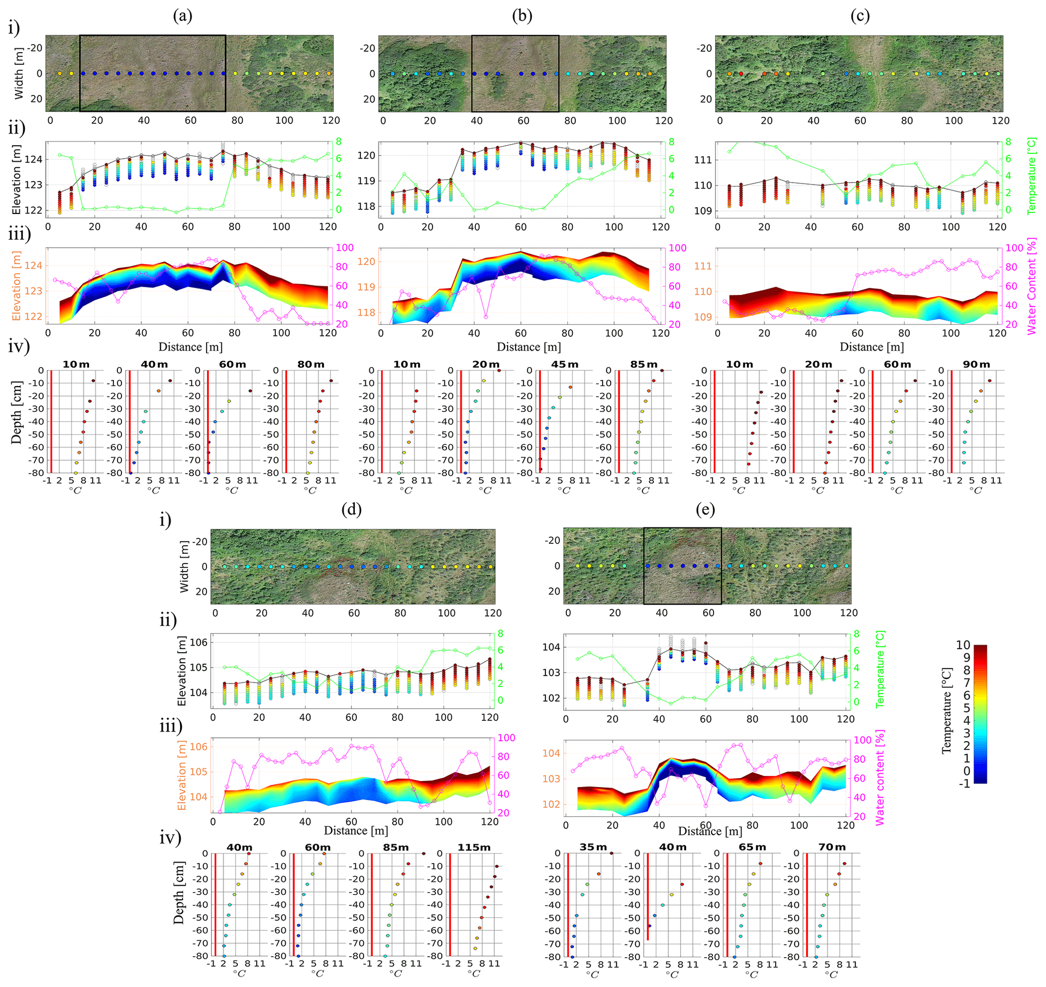
Figure 3DTP data collected on 17 July 2017 along A–E transects. (i) Aerial view of the A–E transects in relative coordinate systems, overlain by temperature at 0.8 m depth and consequently identified near-surface permafrost areas (black rectangles), (ii) DTP temperature profiles and DTP temperature at 0.8 m depth (green line), (iii) interpolated temperature map of the first 0.8 m with topography and surface-water content, and (iv) temperature profiles at selected locations along the transects.
Figure 3 shows each transect in a relative coordinate system in order to accommodate visualizing topography, vegetation type, soil moisture, and the 17 July vertically resolved DTP data together. Based on vertically resolved DTP data, a soil temperature close to or below 0 ∘C at the 0.8 m depth and with a trend in temperature with depth going clearly toward negative temperature values indicates the presence of near-surface permafrost. This is the case between 15 and 75 m along transect A, 40 and 75 m along transect B, and 35 and 65 m along transect E (black rectangles in Fig. 3). The shallowest thaw layer (0.45 m) is observed at 45 m along transect E. This location also corresponds to the lowest temperature at the 0.8 m depth once we extrapolate soil temperature to this depth. The vertical thermal gradient in the top 0.8 m of soil and the measurements of water content in the top 0.3 m using a TDR show sharp changes at a similar location, while their values are not always positively correlated (Fig. 3). Locations identified as near-surface permafrost along transects A and B show high soil water content in the top 0.3 m, while a location identified as near-surface permafrost along transect E shows low water content in the top 0.3 m.
These abrupt lateral changes in soil temperature also correspond to changes in vegetation and topography (Figs. 2 and 3). Figures 2 and 3 suggest that in general the soil temperatures at the 0.8 m depth are the highest under tall-shrub-covered areas (up to 7.5 ∘C), and the lowest under graminoids and dwarf-shrub-dominated areas (down to 0.2 ∘C or below). This general trend is modulated by or intertwined with many factors. The topographic lows along each transect tend to correspond to higher soil temperatures at 0.8 m depths than the topographic highs (Fig. 2). These topographic lows correspond here to preferential drainage paths crossing the transects perpendicularly and are possibly related to ground erosion and/or ground settlement as well as to locations with the higher accumulation of snow during the winter.
In Fig. 4, the soil temperature data are compared to the two long-term thermal monitoring stations (Station 9 and 2 in Fig. 1) to evaluate any potential limitations in interpreting the one-time DTP dataset and to evaluate the value of acquiring spatially dense DTP data. Note that while the DTP system can be deployed for monitoring purposes, here we concentrated on first evaluating its value by acquiring an initial large dataset in July 2017 and later repeating measurements along transects B and C in September 2017. Figure 4a and b show the soil vertical profile of temperatures from the long-term monitoring stations measured at the middle of every month (i.e., every 15th day of the month) from January to September 2017. Figure 4c shows the soil vertical profile of temperature from the long-term monitoring stations overlain on the DTP system measurements along transect A to E in July and transect B and C in September. Soil temperatures at the 0.25 m depth or deeper at Station 9 are lower than at Station 2 year-round. While no temperature measurements are located deeper than the permafrost table at Station 9 and 2, the trend in the temperature data indicates that the permafrost table is likely between 1 and 2 m at Station 9 and much deeper or absent at Station 2. Soil temperature data at Station 2 and 9 are in the upper and lower range of temperature values observed using the DTP system, respectively. Several locations in the DTP dataset show higher and lower temperatures and represent endmembers in the system.
The surficial seasonally frozen layer at Station 2 that developed during the freezing season entirely thawed before 15 June. This observation confirms that the DTP dataset acquired on 17 July is not threatened by potential misinterpretation of near-surface permafrost where a seasonally frozen layer over a thick (>1 m) perennially unfrozen soil is present. At locations where a perennially unfrozen layer is thin or absent, the DTP temperature measurements acquired on 17 July indicate trends in permafrost table depth across the landscape, although a precise estimate of the permafrost table depth cannot be obtained at this time of the year. Furthermore, Station 2 and 9 both show that the vertical profile of temperature has a sharp gradient in the top 0.25 to 0.5 m depth, while at a greater depth the temperature has an increasingly asymptotic behavior. This expected behavior underlines the importance of measuring temperature with the highest vertical resolution close to the surface while still acquiring measurements deeper than 0.5 m where asymptotic trends in soil temperature with depth are more present and strongly informative in the deeper thermal regime.
In Fig. 5, the DTP dataset collected along transects B and C on 20 September is displayed in a similar way to the DTP dataset collected on 17 July in Fig. 3. Figure 5iv shows four of the DTP vertical profiles of soil temperature acquired on 20 September and the corresponding ones collected on 17 July. The DTP soil temperature at the 0.8 m depth measured on 20 September shows a very similar spatial trend (although with different absolute values) to that measured on 17 July, with clearly identifiable near-surface permafrost locations (Figs. 5i and 3i). The air temperature in September is lower than in July, and thus the top 15 cm of soil or more (depending on the location) is colder on 20 September than on 17 July. Compared to 17 July DTP data, the DTP vertical profiles on 20 September show lower thermal gradients, as expected at the end of the summer season. The majority of locations show higher soil temperature in the 0.5 to 0.8 m depth interval on 20 September than on 17 July, while other locations already show the effect of the decrease in downward heat flux at the end of the summer in this interval. The spatiotemporal difference in DTP vertical profiles between 20 September and 17 July, and between the various locations, underlines the complexity of how the heat flux is mediated by soil thermal characteristics in the investigated depth interval as well as by surface and vegetation properties and the thermal regime at a deeper depth than 0.8 m.

Figure 4Temperature profile at Station (a) 9 and (b) 2 at the middle of every month (from 15 January 2017 to 15 September 2017). The 0 ∘C line is in bright red. (c) Comparison of temperature measurements at Station 2 and 9 (solid lines) with DTP measurements (circles) along transects A to E on 17 July (yellow) and along transects B and C on 20 September (orange).
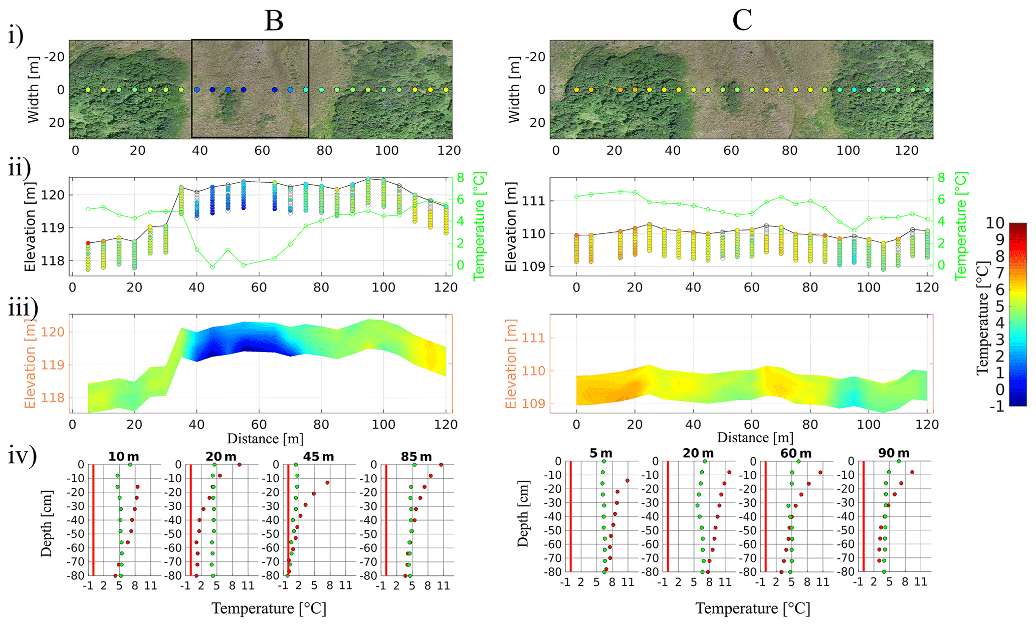
Figure 5DTP data collected on 20 September 2017 along B and C transects. (i) Aerial view and identified near-surface permafrost area (from Fig. 3) overlain by soil temperature at 0.8 m depth, (ii) DTP temperature profiles and DTP temperature at 0.8 m depth (green line), (iii) interpolated temperature map of the first 0.8 m with topography, and (iv) temperature profiles (green dots) at selected locations along the transects and compared to collocated temperature profiles acquired on 17 July (red dots; from Fig. 3).
Figure 6i allows comparison of DTP data at the 0.8 m depth with the ERT data acquired along the same transects at the same time on 17 July 2017. This comparison enables us to assess both the value and the limitations of the DTP system and, in particular, to interpret the vertical extent of near-surface permafrost based on shallow temperature measurements. The ERT transects indicate the presence of large and shallow resistive bodies (up to 104 Ωm, with highest resistivity values in the top 5 m) along transects A and B, which are quite isolated and have sharp lateral resistivity variations. Less resistive zones (approximately lower than 500 Ωm) surround these resistive bodies. The most conductive areas (around 300 Ωm) are located close to the surface and in some cases above the resistive bodies. Transects A and B exhibit the same type of resistivity distribution. Transects D and E have greater similarity to each other than to A and B, except for the shallow resistive area in the middle of transect E. Transect C has a conductive area positioned between deep resistive zones. The near-surface permafrost regions identified in the DTP data (black rectangles in Fig. 3) are collocated with the presence of shallow resistive bodies in the ERT data. This is the case between 15 and 75 m along transect A, 40 and 75 m along transect B, and 35 and 65 m along transect E. While thermo-petrophysical analysis of the ERT data is well beyond the scope of this study, here both the presence of resistive bodies in the ERT data and the collocated presence of low temperature values observed in the top 0.8 m suggest the presence of near-surface permafrost locations.
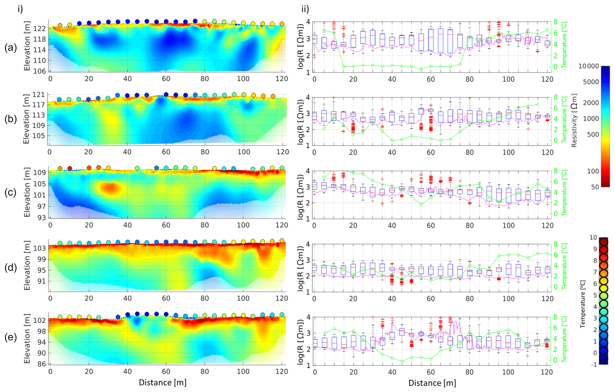
Figure 6(i) ERT data with soil temperature at 0.8 m depth (extracted from the DTP dataset from 17 July 2017) shown at the top of each transect; (ii) boxplots of the resistivity values in the top 7 m depth, vertically averaged resistivity in the top 0.8 m (purple line), and temperature at 0.8 m depth (green line).
The DTP provides the temperature gradient in the top 0.8 m of soil, indicating the potential presence of permafrost at or deeper than this depth interval, while an increase in soil resistivity in the ERT is located where the ground is mostly frozen. Thus, both approaches provide different but complementary information about the depth of permafrost. Figure 6ii shows the DTP dataset at the 0.8 m depth, the top 0.8 m depth average resistivity values for each DTP location, and the range of resistivity values (displayed in a boxplot format) observed over the top 7 m depth in the ERT at each location. The top 0.8 m depth average resistivity value shows a spatial variability relatively similar to the soil water content data, with the exception of depths between 0 and 45 m along transect C. At near-surface permafrost locations, the temperature profiles down to the 0.8 m depth indicate temperature decreasing with depth toward the freezing point (generally located deeper than the 0.8 m depth), while the ERT at a similar depth is widely sensitive to the water content in the thawed layer. The lateral variability in the DTP data at the 0.8 m depth is more consistent with the ERT data when considering the full range of resistivity values observed over the top 7 m in the ERT. Finally, we note that although lateral changes are observed at relatively similar locations in the various properties presented in this study (Figs. 3, 5, and 6), the correlation coefficient for each possible combination of properties across the site is always smaller than 0.5, indicating that no clear linear relationship exists.
In this section, we discuss the information contained in the DTP data and its potential, when coupled with other ground- and aerial-based geophysical datasets, for evaluating the distribution of permafrost.
5.1 Spatial distribution of near-surface permafrost
In environments where topography, soil water content, vegetation, snow thickness, soil-organic-matter content, and other parameters vary strongly over meters to tens of meters, understanding how these properties individually or in combination modulate the heat and water fluxes that influence permafrost distribution and temperature is very challenging. A key advantage of the DTP system is its ability to directly collect spatially dense (horizontal and vertical) soil temperature data. The DTP dataset discussed here provides information important to understanding the ecosystem functioning at the investigated site. First, it directly provides clear identification of near-surface permafrost locations, such as between 15 and 75 m along transect A, 40 and 75 m along transect B, and 35 and 65 m along transect E (Fig. 3). The comparison between the main survey done on 17 July (Fig. 3) and a second survey limited to transect B and C on 20 September (Fig. 5) confirms the general spatial trend in soil temperature and identification of near-surface permafrost locations. The comparison also shows that the lateral extent of the permafrost body along transect B is a few meters smaller than initially identified on 17 July. It is clear that the identification of near-surface permafrost is less prone to uncertainty when performed at the end of the summer. Here, the observed variations along the sides of the near-surface permafrost also indicate the particularly complex spatiotemporal variability in lateral and vertical thermal fluxes occurring at these locations.
The DTP system also provides a spatial resolution that is high enough to observe possible relationships between soil temperature and topographic features, soil water content, and vegetation type. We find that in the study area, near-surface permafrost bodies are always located under topographic highs (at various scales), as seen in Fig. 3. This covariability is in agreement with the expectation that ground settlement will be limited in the presence of near-surface permafrost compared to surrounding locations with deeper or no permafrost. It is also consistent with the fact that topographic lows formed through ground settlement or erosion tend to have thicker snow cover during the winter, which provides more soil insulation and leads to warmer soil thermal conditions compared to topographically high regions (e.g., Wainwright et al., 2017).
Also, the presence of near-surface permafrost identified from the DTP dataset is strongly correlated with the presence of graminoids and/or lichens and dwarf-shrub-covered areas. The graminoid-dominated area crossing transect A (between 15 and 80 m) and B (between 40 and 80 m) can now be considered to encompass a near-surface permafrost body (Fig. 2). The lichen and dwarf-shrub region located along transect E (between 25 and 65 m) is also clearly identified and shows the lateral extent of the near-surface permafrost there.
Furthermore, the soil moisture data suggest that the thaw layer above the near-surface permafrost bodies identified in transects A and B (and collocated with the presence of graminoids) is very wet, if not fully saturated (Fig. 3). We interpret this high soil water content in the thaw layer as being associated with the limited drainage capacity imposed by the topography and the presence of near-surface permafrost. Given the thermal properties of water, one could expect to observe a thicker soil thaw layer where soil is fully water saturated compared to dry soil (Tran et al., 2017). This relationship is clear when comparing the very shallow thaw layer above permafrost (∼0.45 m depth) observed at 45 m along transect E to the area with deeper thaw layer above near-surface permafrost along transects A and B. Indeed, the driest soil is observed at 45 m along transect E (Fig. 3). While this relation is observed between these two locations where near-surface permafrost is present, the soil water content in the thaw layer above the near-surface permafrost along transects A and B is higher than at many other locations where near-surface permafrost is absent. The influence of soil water content on thermal parameters and regime is certain but complex because of water phase changes and soil water content temporal variability controlled by hydraulic parameter and thermal hydrology.
DTP measurements and related identification of near-surface permafrost locations are consistent with ERT data, where high resistivity bodies are identified at similar locations along the transects and at shallow depths (Fig. 6). The high resistivity values observed in the shallow depth (top 4 m) in the ERT are generally located deeper than where the 0 ∘C is expected from the DTP data. This is not unexpected: it can result from (i) smoothness in the ERT inversion, (ii) the presence of still-large unfrozen water content at temperatures between −2 and 0 ∘C, and/or (iii) particularly large unfrozen water content during freezing where the total water content is high.
The combination of DTP data and ERT is also valuable for investigating the subsurface vertical heterogeneity in regions where near-surface permafrost bodies are present. The identified near-surface permafrost bodies extend vertically to about the 15 m depth along transects A and B but much less along transect E, based on the ERT data (Fig. 6). Assuming constant salinity and homogeneous lithology, the ERT suggests that the coldest and most strongly frozen regions of near-surface permafrost bodies occur at depths of about 6 m along transects A and B and at about the 2 m depth along transect E. The DTP data and thaw layer thickness indicate the shallowest top of permafrost along transect E, which is consistent with the ERT data. While temperature in the DTP data could be valuable by itself, adding the ERT in this case enables us to clearly identify locations where near-surface permafrost is thin.
5.2 Beyond the identification of near-surface permafrost locations
While the value and promise of the DTP system for improving our understanding of near-surface permafrost distribution and related shallow lateral and vertical variation in temperature regimes are demonstrated in the previous section, the variations in soil temperature, where deep permafrost – with a perennially thawed zone above it – or no permafrost is present, are more difficult to interpret.
When surface-water content is high and the permafrost table is deep or permafrost is absent, the thermal profile shows relatively low temperatures right below the surface, with a relatively small vertical temperature gradient. This is the case between 0 and 70 m along transect D and between 0 and 30 and 65 and 120 m along transect E (Fig. 3). These locations are at the flat toe of the hillslope, with the groundwater table at or very close to the surface. The soil temperature at these locations is around 1–2 ∘C at the 0.80 m depth and possibly decreases below 0 ∘C at much greater depths. We interpret the large soil water content and some water inundation to be maintaining a relatively homogeneous and stable shallow temperature regime, owing to the water's high heat capacity. In such a wet environment, the latent heat effect is likely reinforced as well. The melting pore ice can absorb additional heat and slow the rate of temperature increase. Similarly, as temperature decreases in autumn, freezing pore water releases latent heat and slows temperature decline (Osterkamp and Romanovsky, 1997; Shojae Ghias et al., 2017). At such locations, the DTP data indicate that a perennially thawed zone may be present along with the possible presence of deeper permafrost.
Another interesting case is along transect C (Fig. 3) between 0 and 30 m. At this location, the DTP data show a very small thermal gradient between the surface and the 0.8 m depth, where the temperature is still as high as ∼7 ∘C. In addition, this location has a ground elevation that is slightly higher than the rest of the transect, is relatively dry at the surface, is situated in tall-shrub area where snow depth may be large during the winter, and is interpreted to have some rocky soil based on probe installation. This relatively dry and rocky location suggests that the soil in this region has a low heat capacity, which would decrease the ability of soil to maintain its temperature in the surveyed depth interval and produce a small thermal gradient as observed here. This is confirmed by the 20 September DTP data between 0 and 30 m along transect C (Fig. 5iv) showing lower soil temperatures in the entire 0–0.8 m surveyed depth interval (compared to 17 July), which indicates that the lower air temperature in September likely had already a strong influence on the entire temperature profile. This is different from most of the other locations, which show an increase in soil temperature at the 0.8 m depth between 17 July and 20 September. In addition to dry and rocky material that could explain the limited ability of soil to maintain its temperature in the surveyed depth interval, a change in soil thermal parameters below the surveyed depth interval may further impede the transfer of heat to a deeper layer. At this time, we cannot confirm if the deeper layer, which indeed is resistive in the ERT data, was permafrost or bedrock. The end of transects A and B most likely exhibits the same physical process discussed above, in which the shallow temperature is relatively high and water content relatively low, producing higher uncertainty regarding permafrost presence at depths greater than 4 m.
The aforementioned results, and the complexity involved in how heat flux is modulated by various surface properties and soil heterogeneity, underscore the importance of surveying numerous locations and measuring soil temperature profiles down to the 0.8 m depth or deeper, ideally over time. The DTP system and the long-term monitoring Station 2 and 9 show that measuring only the very shallow surface temperature (first 30 cm) is insufficient for evaluating deeper thermal regimes (Fig. 4). Temporal variations in soil temperature in the top 10 to top 30 cm can be significant over short periods of time (up to the hour scale) and not representative of deeper thermal regimes, especially in dry areas. In addition, the strong decay in temperature in the top 30 cm can produce larger error within temperature data in the case of uncertainty as to the exact depth where the point sensor is located. This expected behavior, based on the physics of thermal flux, confirms the need for measuring temperature with high vertical resolution close to the surface as well as at depths deeper than 0.5 m, where asymptotic trends in soil temperature at depth are more present. In addition, the comparison of 17 July and 20 September surveys (Fig. 5) shows that observing the system over time provides, as expected, very valuable information to go beyond the identification of near-surface permafrost. The DTP dataset will clearly benefit from year-round acquisition of soil temperature measurements at different depths, which are key for the interpretation of both surface energy balance and deeper thermal characteristics and regimes. High vertical resolution close to the surface (Fig. 3) has the potential to provide information on freezing or thawing fronts in shoulder seasons as well as on the influence of organic layers on deeper thermal regimes.
Finally, based on the long-term monitoring station data (Fig. 4), we expect that obtaining the fluctuation in temperature over time using the DTP will improve the ability to evaluate various regimes and factors. We also expect the time-lapse soil measurements to be useful as input to inverse modeling techniques focused on estimating soil thermal parameters and possibly soil-organic-matter content (e.g., Nicolsky et al., 2009; Tran et al., 2017).
This study describes a novel strategy referred to as distributed temperature profiling (DTP) to quantify the near-surface soil thermal state at an unprecedented number of depths and locations and test this approach for the delineation of near-surface permafrost regions in a discontinuous permafrost environment by moving the DTP system sequentially across the landscape. To our knowledge, this is the first time that a thermal characterization approach has provided such high vertical and lateral density in measurements. The low cost, portability, and ease of deploying the DTP system makes this method efficient for investigating permafrost spatial heterogeneity, particularly where significant lateral variations in soil temperature occur over meters to tens of meters. As shown, the densely spaced DTP data compared well with classical thermal measurements and provided much higher spatial resolution. Possible deployment of DTP systems in a time-lapse mode will also enable high temporal resolution and larger temporal coverage.
In this study, the DTP dataset has shown to be particularly valuable in delineating the presence of near-surface permafrost. When combined with other approaches, the DTP was also useful for evaluating correspondences between summer soil temperature, plant type, topography, soil water content, and deeper subsurface structure. Since decoupling the control of these and other factors (e.g., organic content and snow depth) on thaw layer thickness and the depth of permafrost table is complex and beyond the scope of this paper, our data indicate that changes in soil temperatures often correspond to changes in topography, vegetation, and soil moisture. Near-surface permafrost identified in the study area using the DTP data is primarily collocated under topographic highs and under areas covered with graminoids or lichens and dwarf shrubs. The results provide new insights about the presence or absence of near-surface permafrost bodies.
The simple and low-cost DTP strategy holds promise for improving our ability to quantify local permafrost distribution and to explore interactions between complex Arctic ecosystem properties and processes. In particular, coupling various observations has the potential to advance strategies to estimate permafrost distribution from remotely sensed information, including topography, vegetation, and possibly surficial moisture characteristics. This study opens the door to such quantification, although many challenges remain. For example, while covariability is observed between near-surface permafrost and topographic highs and the absence of tall shrubs, multiple factors need to be accounted and estimated for possibly identifying these from remote-sensing data. It includes automated extraction of topographic information at various scales as well as the identification of physical vegetation, snow, and soil characteristics.
Ongoing developments in the DTP system include the miniaturization and cost reduction of the data logger, improvement and cost reduction of the temperature probe fabrication, ability to produce probes with variable length and vertical resolution, development of open-source software and hardware to encourage community-based development and deployment, and automated acquisition and data transfer for long-term monitoring purposes. These developments will enable the deployment of low-cost DTP to measure and record ground temperatures year-round and with a number of probes that are well beyond those described in this study. The potential of this method for characterizing and monitoring a variety of near-surface heat and related water dynamic processes is significant for informing investigations aimed at quantifying water infiltration, evaporation, biogeochemical processes, hyporheic exchange, snowmelt dynamics, and permafrost evolution.
All data used in the analysis presented here are available by contacting the corresponding author or at https://doi.org/10.5440/1559886 (Dafflon et al., 2019).
EL and BD developed the acquisition strategy, conducted the tool development and the data acquisition and analysis, and prepared the paper. YR assisted with the development, acquisition, and analysis. CU, JP, and SB assisted with data acquisition. VR and SH assisted with developing acquisition strategy and preparing the paper.
The authors declare that they have no conflict of interest.
We acknowledge the assistance of Todd Wood, Paul Cook, and Alejandro Morales of the Geoscience Measurement Facility (GMF) at Lawrence Berkeley National Laboratory for building the DTP prototype system. The probe sleeve and filling material were partly influenced by the work of Bill Cable (UAF, Alaska).
This research has been supported by the Office of Biological and Environmental Research in the DOE Office of Science (grant no. DE-AC02-05CH11231).
This paper was edited by Ketil Isaksen and reviewed by two anonymous referees.
Alcoforado, M.-J. and Andrade, H.: Nocturnal urban heat island in Lisbon (Portugal): main features and modelling attempts, Theor. Appl. Climatol., 84, 151–159, 2006.
Ashton, K.: That “Internet of Things” thing, J. RFID, 22, 97–114, 2009.
Binley, A. and Kemna, A.: DC Resistivity and Induced Polarization Methods, in: Hydrogeophysics, edited by: Rubin, Y. and Hubbard, S. S., Springer Netherlands, 2005.
Biskaborn, B. K., Lanckman, J.-P., Lantuit, H., Elger, K., Streletskiy, D. A., Cable, W. L., and Romanovsky, V. E.: The new database of the Global Terrestrial Network for Permafrost (GTN-P), Earth Syst. Sci. Data, 7, 245–259, https://doi.org/10.5194/essd-7-245-2015, 2015.
Brewer, M. C.: The thermal regime of an Arctic lake, Eos, Transactions American Geophysical Union, 39, 278–284, 1958.
Briggs, M. A., Lautz, L. K., McKenzie, J. M., Gordon, R. P., and Hare, D. K.: Using high-resolution distributed temperature sensing to quantify spatial and temporal variability in vertical hyporheic flux, Water Resour. Res., 48, W02527, https://doi.org/10.1029/2011WR011227, 2012.
Burn, C. R.: Tundra lakes and permafrost, Richards Island, western Arctic coast, Canada, Can. J. Earth Sci., 39, 1281–1298, 2002.
Cable, W. L., Romanovsky, V. E., and Jorgenson, M. T.: Scaling-up permafrost thermal measurements in western Alaska using an ecotype approach, The Cryosphere, 10, 2517–2532, https://doi.org/10.5194/tc-10-2517-2016, 2016.
Dafflon, B., Hubbard, S., Ulrich, C., Peterson, J., Wu, Y., Wainwright, H., and Kneafsey, T. J.: Geophysical estimation of shallow permafrost distribution and properties in an ice-wedge polygon-dominated Arctic tundra region, GEOPHYSICS, 81, WA247–WA263, 2016.
Dafflon, B., Oktem, R., Peterson, J., Ulrich, C., Tran, A. P., Romanovsky, V., and Hubbard, S. S.: Coincident aboveground and belowground autonomous monitoring to quantify covariability in permafrost, soil, and vegetation properties in Arctic tundra, J. Geophys. Res.-Biogeosci., 122, 1321–1342, 2017.
Dafflon, B., Leger, E., and Hubbard, S.: Characterization of Soil Thermal and Electrical Properties along Multiple Hillslope Transects at Teller Road Site, Seward Peninsula, Alaska, 2017, Next Generation Ecosystem Experiments Arctic Data Collection, Oak Ridge National Laboratory, U.S. Department of Energy, Oak Ridge, Tennessee, USA, https://doi.org/10.5440/1559886, 2019.
Davesne, G., Fortier, D., Domine, F., and Gray, J. T.: Wind-driven snow conditions control the occurrence of contemporary marginal mountain permafrost in the Chic-Choc Mountains, south-eastern Canada: a case study from Mont Jacques-Cartier, The Cryosphere, 11, 1351–1370, https://doi.org/10.5194/tc-11-1351-2017, 2017.
Davidson, E. A. and Janssens, I. A.: Temperature sensitivity of soil carbon decomposition and feedbacks to climate change, Nature, 440, 165–173, 2006.
Dougherty, D.: The maker movement, Innovations, 7, 11–14, 2012.
Fang, C. and Moncrieff, J. B.: The dependence of soil CO2 efflux on temperature, Soil Biol. Biochem., 33, 155–165, 2001.
Gisnås, K., Westermann, S., Schuler, T. V., Litherland, T., Isaksen, K., Boike, J., and Etzelmüller, B.: A statistical approach to represent small-scale variability of permafrost temperatures due to snow cover, The Cryosphere, 8, 2063–2074, https://doi.org/10.5194/tc-8-2063-2014, 2014.
Goyanes, G., Vieira, G., Caselli, A., Cardoso, M., Marmy, A., Santos, F., Bernardo, I., and Hauck, C.: Local influences of geothermal anomalies on permafrost distribution in an active volcanic island (Deception Island, Antarctica), Geomorphology, 225, 57–68, 2014.
Gubler, S., Fiddes, J., Keller, M., and Gruber, S.: Scale-dependent measurement and analysis of ground surface temperature variability in alpine terrain, The Cryosphere, 5, 431–443, https://doi.org/10.5194/tc-5-431-2011, 2011.
Guglielmin, M.: Ground surface temperature (GST), active layer and permafrost monitoring in continental Antarctica, Permafr. Perigl. Process., 17, 133–143, 2006.
Harris, C., Haeberli, W., Vonder Mühll, D., and King, L.: Permafrost monitoring in the high mountains of Europe: the PACE project in its global context, Permafr. Perigl. Process., 12, 3–11, 2001.
Hauck, C.: Frozen ground monitoring using DC resistivity tomography, Geophys. Res. Lett., 29, 12-11–12-14, 2002.
Hausner, M. B., Suarez, F., Glander, K. E., van de Giesen, N., Selker, J. S., and Tyler, S. W.: Calibrating Single-Ended Fiber-Optic Raman Spectra Distributed Temperature Sensing Data, Sensors, 11, 10859–10879, 2011.
Hilbich, C., Hauck, C., Hoelzle, M., Scherler, M., Schudel, L., Völksch, I., Mühll, D. V., and Mäusbacher, R.: Monitoring mountain permafrost evolution using electrical resistivity tomography: A 7–year study of seasonal, annual, and long–term variations at Schilthorn, Swiss Alps, J. Geophys. Res.-Earth Surf., 113, F01S90, https://doi.org/10.1029/2007JF000799, 2008.
Holden, Z. A., Swanson, A., Klene, A. E., Abatzoglou, J. T., Dobrowski, S. Z., Cushman, S. A., Squires, J., Moisen, G. G., and Oyler, J. W.: Development of high-resolution (250 m) historical daily gridded air temperature data using reanalysis and distributed sensor networks for the US Northern Rocky Mountains, Int. J. Climatol., 36, 3620–3632, 2016.
Hopkins, D. M. and Karlstrom, T. N. V.: Permafrost and ground water in Alaska. Geological Survey Professional Paper, 1955.
Hubbard, S. S., Gangodagamage, C., Dafflon, B., Wainwright, H., Peterson, J., Gusmeroli, A., Ulrich, C., Wu, Y., Wilson, C., Rowland, J., Tweedie, C., and Wullschleger, S.: Quantifying and relating land-surface and subsurface variability in permafrost environments using LiDAR and surface geophysical datasets, Hydrogeol. J., 21, 149–169, 2013.
Hubbart, J., Link, T., Campbell, C., and Cobos, D.: Evaluation of a low-cost temperature measurement system for environmental applications, Hydrol. Process., 19, 1517–1523, 2005.
Isaksen, K., Ødegård, R. S., Etzelmüller, B., Hilbich, C., Hauck, C., Farbrot, H., Eiken, T., Hygen, H. O., and Hipp, T. F.: Degrading mountain permafrost in southern Norway: spatial and temporal variability of mean ground temperatures, 1999–2009, Permafr. Perigl. Process., 22, 361–377, 2011.
Jafarov, E., Coon, D. T., Harp, D. R., Wilson, C. J., Painter, S. L., Atchley, A. L., and Romanovsky, V. E.: Modeling the role of preferential snow accumulation in through talik development and hillslope groundwater flow in a transitional permafrost landscape, Environ. Res. Lett., 13, 105006, https://doi.org/10.1088/1748-9326/aadd30, 2018.
Jorgenson, M. T., Romanovsky, V., Harden, J., Shur, Y., O'Donnell, J., Schuur, E. A. G., Kanevskiy, M., and Marchenko, S.: Resilience and vulnerability of permafrost to climate change, Can. J. Forest Res., 40, 1219–1236, 2010.
Krautblatter, M., Verleysdonk, S., Flores-Orozco, A., and Kemna, A.: Temperature-calibrated imaging of seasonal changes in permafrost rock walls by quantitative electrical resistivity tomography (Zugspitze, German/Austrian Alps), J. Geophys. Res.-Earth Surf., 115, F02003, https://doi.org/10.1029/2008JF001209, 2010.
Lachenbruch, A. and Marshall, B.: Heat Flow in the Arctic, ARCTIC, 22, 300–311, 1969.
Léger, E., Dafflon, B., Soom, F., Peterson, J., Ulrich, C., and Hubbard, S.: Quantification of Arctic Soil and Permafrost Properties Using Ground-Penetrating Radar and Electrical Resistivity Tomography Datasets, IEEE J. Select. Top. Appl. Earth Observ. Remote Sens., 10, 4348–4359, 2017.
Lewkowicz, A. G., Bonnaventure, P. P., Smith, S. L., and Kuntz, Z.: Spatial and thermal characteristics of mountain permafrost, northwest canada, Geograf. Ann. Series A, 94, 195–213, 2012.
Lundquist, J. D. and Lott, F.: Using inexpensive temperature sensors to monitor the duration and heterogeneity of snow-covered areas, Water Resour. Res., 44, W00D16, https://doi.org/10.1029/2008WR007035, 2008.
Marescot, L., Monnet, R. E., gis, and Chapellier, D.: Resistivity and induced polarization surveys for slope instability studies in the Swiss Alps, Eng. Geol., 98, 18–28, https://doi.org/10.1016/j.enggeo.2008.01.010, 2008.
Minsley, B. J., Abraham, J. D., Smith, B. D., Cannia, J. C., Voss, C. I., Jorgenson, M. T., Walvoord, M. A., Wylie, B. K., Anderson, L., Ball, L. B., Deszcz-Pan, M., Wellman, T. P., and Ager, T. A.: Airborne electromagnetic imaging of discontinuous permafrost, Geophys. Res. Lett., 39, L02503, https://doi.org/10.1029/2011GL050079, 2012.
Mukhopadhyay, S. C.: Intelligent sensing, instrumentation and measurements, Springer, 2013.
Nelson, F., Outcalt, S., Brown, J., Shiklomanov, N., and Hinkel, K.: Spatial and temporal attributes of the active layer thickness record, Barrow, Alaska, USA, Proceedings of the Seventh International Conference on Permafrost, Yellowknife NWT, 797–802, 1998.
Nicolsky, D. J., Romanovsky, V. E., and Panteleev, G. G.: Estimation of soil thermal properties using in-situ temperature measurements in the active layer and permafrost, Cold Reg. Sci. Technol., 55, 120–129, 2009.
Osterkamp, T. E.: Response of Alaskan permafrost to climate, Proceedings of the Fourth International Conference on Permafrost, Fairbanks, 17–22 July, 145–152, 1983.
Osterkamp, T. E.: Temperature measurement in Permafrost, Alaska DOTPF, Fairbanks, AK, 87 pp., 1985.
Osterkamp, T. E.: Freezing and thawing of soils and permafrost containing unfrozen water or brine, Water Resour. Res., 23, 2279–2285, 1987.
Osterkamp, T. E. and Gosink, J. P.: Variations in permafrost thickness in response to changes in paleoclimate, J. Geophys. Res.-Solid Earth, 96, 4423–4434, 1991.
Osterkamp, T. E. and Romanovsky, V. E.: Freezing of the Active Layer on the Coastal Plain of the Alaskan Arctic, Permafr. Perigl. Process., 8, 23–44, 1997.
Roger, J., Allard, M., Sarrazin, D., L'Hérault, E., Doré, G., and Guimond, A.: Evaluating the use of distributed temperature sensing for permafrost monitoring in Salluit, Nunavik, 68th Canadian geotechnical conference and 7th Canadian permafrost conference; GEOQuébec 2015, Vancouver, BC, Canada, 2015.
Romanovsky, V. E. and Osterkamp, T. E.: Interannual variations of the thermal regime of the active layer and near-surface permafrost in northern Alaska, Permafr. Perigl. Process., 6, 313–335, 1995.
Romanovsky, V. E. and Osterkamp, T. E.: Effects of unfrozen water on heat and mass transport processes in the active layer and permafrost, Permafr. Perigl. Process., 11, 219–239, 2000.
Rowland, J. C., Travis, B. J., and Wilson, C. J.: The role of advective heat transport in talik development beneath lakes and ponds in discontinuous permafrost, Geophys. Res. Lett., 38, L17504, https://doi.org/10.1029/2011GL048497, 2011.
Rücker, T. G. C. and Spitzer, K.: 3-d modeling and inversion of DC resistivity data incorporating topography – Part II: Inversion, Geophys. J. Int., 166, 506–517, 2006.
Rücker, C., Günther, T., and Spitzer, K.: 3-d modeling and inversion of DC resistivity data incorporating topography – Part I: Modeling, Geophys. J. Int., 166, 495–505, 2006.
Rücker, C., Günther, T., and Wagner, F. M.: pyGIMLi: An open-source library for modelling and inversion in geophysics, Comput. Geosci., 109, 106–123, 2017.
Schön, J. H.: Physical properties of rocks: Fundamentals and principles of petrophysics, Elsevier, 2015.
Shiklomanov, N., Nelson, F., Streletskiy, D., Hinkel, K., and Brown, J.: The circumpolar active layer monitoring (CALM) program: data collection, management, and dissemination strategies, Proceedings of the Ninth International Conference on Permafrost, 29 June–3 July 2008, 2008.
Shojae Ghias, M., Therrien, R., Molson, J., and Lemieux, J.-M.: Controls on permafrost thaw in a coupled groundwater-flow and heat-transport system: Iqaluit Airport, Nunavut, Canada, Hydrogeol. J., 25, 657–673, 2017.
Smits, K. M., Cihan, A., Sakaki, T., and Illangasekare, T. H.: Evaporation from soils under thermal boundary conditions: Experimental and modeling investigation to compare equilibrium- and nonequilibrium-based approaches, Water Resour. Res., 47, W05540, https://doi.org/10.1029/2010WR009533, 2011.
Stieglitz, M., Dèry, S. J., Romanovsky, V. E., and Osterkamp, T. E.: The role of snow cover in the warming of arctic permafrost, Geophys. Res. Lett., 30, 1721, https://doi.org/10.1029/2003GL017337, 2003.
Stonestrom, D. A. and Constantz, J. (Eds.): Heat as a tool for studying the movement of ground water near streams, U.S. Geol. Surv. Circ, 2003.
Sturm, M., Racine, C., and Tape, K.: Increasing shrub abundance in the Arctic, Nature, 411, 546–547, 2001.
Swartz, J. H.: A geothermal measuring circuit, Science, 120, 573–574, 1954.
Till, A., Dumoulin, J. A., Gamble, B., Kaufman, D., and Carroll, P.: Preliminary geologic map and fossil data, Solomon, Bendeleben, and southern Kotzebue quadrangles, Seward Peninsula, Alaska, US Geological Survey, 2331–1258, 1986.
Tran, A. P., Dafflon, B., and Hubbard, S. S.: Coupled land surface-subsurface hydrogeophysical inverse modeling to estimate soil organic carbon content and explore associated hydrological and thermal dynamics in the Arctic tundra, The Cryosphere, 11, 2089–2109, https://doi.org/10.5194/tc-11-2089-2017, 2017.
Tyler, S. W., Selker, J. S., Hausner, M. B., Hatch, C. E., Torgersen, T., Thodal, C. E., and Schladow, S. G.: Environmental temperature sensing using Raman spectra DTS fiber-optic methods, Water Resour. Res., 45, W00d23, https://doi.org/10.1029/2008WR007052, 2009.
Wagner, A. M., Lindsey, N. J., Dou, S., Gelvin, A., Saari, S., Williams, C., Ekblaw, I., Ulrich, C., Borglin, S., Morales, A., and Ajo-Franklin, J.: Permafrost Degradation and Subsidence Observations during a Controlled Warming Experiment, Sci. Rep., 8, 1–9, 2018.
Wainwright, H. M., Dafflon, B., Smith, L. J., Hahn, M. S., Curtis, J. B., Wu, Y., Ulrich, C., Peterson, J. E., Torn, M. S., and Hubbard, S. S.: Identifying multiscale zonation and assessing the relative importance of polygon geomorphology on carbon fluxes in an Arctic tundra ecosystem, J. Geophys. Res.-Biogeosci., 120, 788–808, 2015.
Wainwright, H. M., Liljedahl, A. K., Dafflon, B., Ulrich, C., Peterson, J. E., Gusmeroli, A., and Hubbard, S. S.: Mapping snow depth within a tundra ecosystem using multiscale observations and Bayesian methods, The Cryosphere, 11, 857–875, https://doi.org/10.5194/tc-11-857-2017, 2017.
Whiteman, C. D., Hubbe, J. M., and Shaw, W. J.: Evaluation of an inexpensive temperature datalogger for meteorological applications, J. Atmos. Ocean. Technol., 17, 77–81, 2000.
Wu, Y., Hubbard, S. S., Ulrich, C., and Wullschleger, S. D.: Remote monitoring of freeze – thaw transitions in Arctic soils using the complex resistivity method, Vadose Zone J., 12, 1–13, 2013.
Yoshikawa, K. and Hinzman, L. D.: Shrinking thermokarst ponds and groundwater dynamics in discontinuous permafrost near Council, Alaska, Permafr. Perigl. Process., 14, 151–160, 2003.
Zhang, T.: Influence of the seasonal snow cover on the ground thermal regime: An overview, Rev. Geophys., 43, RG4002, https://doi.org/10.1029/2004RG000157, 2005.
Zhang, T., Osterkamp, T. E., and Stamnes, K.: Some Characteristics of the Climate in Northern Alaska, U. S. A., Arct. Alpine Res., 28, 509–518, 1996.