the Creative Commons Attribution 4.0 License.
the Creative Commons Attribution 4.0 License.
 | 08 Nov 2019
Estimating early-winter Antarctic sea ice thickness from deformed ice morphology
Ted Maksym
Blake Weissling
Hanumant Singh
Satellites have documented variability in sea ice areal extent for decades, but there are significant challenges in obtaining analogous measurements for sea ice thickness data in the Antarctic, primarily due to difficulties in estimating snow cover on sea ice. Sea ice thickness (SIT) can be estimated from snow freeboard measurements, such as those from airborne/satellite lidar, by assuming some snow depth distribution or empirically fitting with limited data from drilled transects from various field studies. Current estimates for large-scale Antarctic SIT have errors as high as ∼50 %, and simple statistical models of small-scale mean thickness have similarly high errors. Averaging measurements over hundreds of meters can improve the model fits to existing data, though these results do not necessarily generalize to other floes. At present, we do not have algorithms that accurately estimate SIT at high resolutions. We use a convolutional neural network with laser altimetry profiles of sea ice surfaces at 0.2 m resolution to show that it is possible to estimate SIT at 20 m resolution with better accuracy and generalization than current methods (mean relative errors ∼15 %). Moreover, the neural network does not require specification of snow depth or density, which increases its potential applications to other lidar datasets. The learned features appear to correspond to basic morphological features, and these features appear to be common to other floes with the same climatology. This suggests that there is a relationship between the surface morphology and the ice thickness. The model has a mean relative error of 20 % when applied to a new floe from the region and season. This method may be extended to lower-resolution, larger-footprint data such as such as Operation IceBridge, and it suggests a possible avenue to reduce errors in satellite estimates of Antarctic SIT from ICESat-2 over current methods, especially at smaller scales.


Satellites have documented changes in sea ice extent (SIE) for decades (Parkinson and Cavalieri, 2012); however, sea ice thickness (SIT) is much harder to measure remotely. Declines in Arctic SIT over the past several decades have been detected in under-ice upward-looking sonar surveys and satellite observations (Rothrock et al., 2008; Kwok and Rothrock, 2009). Arctic ice thickness has been observed with satellite altimetry to continue to decline over the past decade (Kwok and Cunningham, 2015), but any possible trends in Antarctic SIT are difficult to detect because of the presumably relatively small changes, and difficulties in estimating SIT in the Antarctic (Kurtz and Markus, 2012; Zwally et al., 2008). Because fully coupled models generally fail to reproduce the observed multi-decadal increase in Antarctic SIE, it is likely that their simulated decrease in Antarctic SIT is also incorrect (Turner et al., 2013; Shu et al., 2015). However, ocean–ice models forced with atmospheric reanalysis correctly reproduce an increasing Antarctic SIE and suggest an increasing SIT (Holland et al., 2014). Massonnet et al. (2013) found that assimilating sea ice models with sea ice concentration shows that SIT covaries positively with SIE at the multi-decadal timescale and thus implies an increasing sea ice volume in the Antarctic. Detection of variations in SIT and volume are important to understanding a variety of climate feedbacks (e.g., Holland et al., 2006; Stammerjohn et al., 2008); for example, they are critical to understanding trends and variability in Southern Ocean salinity (e.g., Haumann et al., 2016). At present, large-scale ice thickness cannot be retrieved with sufficient accuracy to detect with any confidence the relatively small trends in thickness expected (Massonnet et al., 2013), or even interannual variability (Kern and Spreen, 2015).
The main source of Antarctic SIT measurements comes from ship-based visual observations (ASPeCt, the Antarctic Sea-ice Processes and Climate, compiled in Worby et al., 2008), drill-line measurements (e.g., Tin and Jeffries, 2003; Ozsoy-Cicek et al., 2013), aerial surveys with electromagnetic induction (e.g., Haas et al., 2009) and sporadic data from moored upward-looking sonar (ULS) (e.g., Worby et al., 2001; Harms et al., 2001; Behrendt et al., 2013). These are all sparsely conducted, with significant gaps in both time and space, making it hard to infer any variability or trends. There is also some evidence of a sampling bias towards thinner ice due to logistical constraints of ships traversing areas of thick and deformed ice (Williams et al., 2015).
The only currently feasible means of obtaining SIT data on a large enough scale to examine thickness variability is through remotely sensed data, from either large-scale airborne campaigns such as Operation IceBridge (OIB) (Kurtz, 2013) or more broadly from satellite altimetry, (e.g., ICESat, Zwally et al., 2008, or more recently, ICESat-2, Markus et al., 2017). Here, SIT is derived from either the measured snow surface (i.e., surface elevation referenced to local sea level) in the case of laser altimeters (ICESat and OIB) or a measure of the ice surface freeboard (CryoSat-2) (Wingham et al., 2006). The measurement of the surface elevation itself has some error, due to the error in estimating the local sea surface height (Onana et al., 2012). When using radar altimetry, the ice–snow interface may be hard to detect as observations suggest that the radar return can occur from within the snowpack (e.g., Willatt et al., 2009), possibly due to scattering from brine wicked up into the overlying snow, melt–freeze cycles creating ice lenses, or from the snow–ice interface (Fons and Kurtz, 2019). However, even with an accurate measurement of the snow–ice freeboard, there are challenges with converting this to a SIT estimate.
Assuming hydrostatic equilibrium, the ice thickness T may be related to the snow freeboard F (i.e., snow depth + ice freeboard; see Fig. 1) and snow depth D measurements using the relation
for some densities of ice, water and snow (Fig. 1). Without simultaneous snow depth estimates (e.g., from passive microwave radiometry (Markus and Cavalieri, 1998) or from ultra-wideband snow radar such as that used on OIB (e.g., Kwok and Maksym, 2014), some assumption of snow depth has to be made, or an empirical fit to field observations is needed (e.g., Ozsoy-Cicek et al., 2013). When averaging over multiple kilometers, and in particular during spring, it is common to assume that there is no ice component in the snow freeboard, i.e., F=D in Eq. (1) (Xie et al., 2013; Yi et al., 2011; Kurtz and Markus, 2012). However, this assumption is likely not valid near areas of deformed ice, which may have significant nonzero ice freeboard, and OIB data suggest this is not true at least for much of the spring sea ice pack (Kwok and Maksym, 2014). More generally, empirical fits of SIT to F can be used (Ozsoy-Cicek et al., 2013), but these implicitly assume a constant proportion of snow within the snow freeboard and a constant snow and ice density. These are not likely to be true, particularly at smaller scales and for deformed ice. Moreover, detecting variability with such methods is prone to error because these relationships may change seasonally and interannually. Kern and Spreen (2015) suggested a ballpark error of 50 % from ICESat-derived thickness estimates. Kern et al. (2016), following Worby et al. (2008), looked at the snow freeboard as one layer with some effective density taken as some linear combination of sea ice and snow densities. More recently, Li et al. (2018) have used a regionally and temporally varying density (equivalently, a variable proportion of snow in snow freeboard) inferred from the empirical fits of Ozsoy-Cicek et al. (2013), which is equivalent to a more complex, regime-dependent set of snow assumptions.
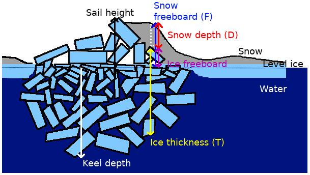
Figure 1A schematic diagram of a typical first-year ridge. The ridge may not be symmetric, and peaks of the sail and keel may not coincide. The effective density of the ice is affected by the air gaps above water and the water gaps below water. T, D and F may be linked by assuming hydrostatic balance (Eq. 1).
A key question is how much the sea ice morphology affects these relationships between surface measurements and thickness. Pressure ridges, which form when sea ice collides, fractures and forms a mound-like structure (Fig. 1), are a primary source of deformed ice. Although only a minority of the sea ice surface is deformed, ridges occur at a spatial frequency of 3–30 per kilometer and so may account for a majority of the total sea ice volume (Worby et al., 1996; Haas et al., 1999). The sea ice surface naturally has a varying proportion of deformed ice, which affects the sampling required to faithfully represent the distribution (Weissling and Ackley, 2011). Around deformed areas, both the ice freeboard and snow depth may be high, and we do not yet know the statistical distribution of snow around such deformation features. In this respect, local estimates of SIT are likely biased low as the average ice freeboard cannot be assumed to be zero. Moreover, the effective density of deformed ice (i.e., the density of the deformed ice including snow-, air- and seawater-filled gaps) may differ significantly from level ice areas due to drained brine and trapped snow in ridge sails and seawater in large pore spaces in ridge keels (Fig. 1; also discussed in Hutchings et al., 2015). Because these densities affect the empirical fits, it is important to quantify how SIT predictions should be adjusted to account for morphological differences in snow freeboard measurements.
Many pressure ridges can be observed from above using airborne or terrestrial lidar scans (e.g., Dierking, 1995). However, it is difficult to derive SIT of deformed areas from these scans due to the difficulty in determining the contribution of snow to the snow freeboard measured by a lidar scan. Furthermore, the corresponding keel morphology given some surface (lidar) scan, and its effect on the SIT distribution, is not known. Among other factors, radar-based estimates of snow depth are known to be highly sensitive to surface roughness, weather and grain size (Stroeve et al., 2006; Markus and Cavalieri, 1998). Ozsoy-Cicek et al. (2011) and Markus et al. (2011) found that snow depth measured by the Advanced Microwave Scanning Radiometer – Earth Observing System (AMSR-E) around deformed ice is underestimated by a factor of 2 or more. Kern and Spreen (2015) also showed that the error estimate in the SIT is considerably affected by the snow depth error, with a conservative estimate of 30 % error in snow depth leading to a relative ice thickness error up to 80 %.
Sea ice draft and ridge morphology may also be observed from below using sonar on autonomous underwater vehicles (AUVs) (e.g., Williams et al., 2015). Although AUV datasets of deformed ice have higher resolution than airborne and satellite-borne lidar datasets, they are much more sparsely conducted and fewer such datasets of Antarctic ice exist. This makes it hard to generalize conclusions of deformed sea ice from empirical datasets. It is therefore important to understand how the morphology of deformed ice relates to its thickness distribution. By using coincident, high-resolution, and three-dimensional AUV and lidar surveys of deformed ice, we can characterize areas of deformation and surface morphology and their relationship to ice thickness and snow freeboard much better than with linear, low-resolution drilling profiles.
In order to account for the varying effective density of a ridge, we need to be able to characterize different deformed surfaces. The analysis of ridge morphology is currently very simplistic. As summarized in Strub-Klein and Sudom (2012), the geometry of the above-water (sail) and below-water (keel) heights is typically analyzed, traditionally by calculating the sail–keel ratios and sail angles (Timco and Burden, 1997). There are known morphological differences between Arctic and Antarctic ridges, such as sail heights of Antarctic ridges being generally lower than those of Arctic ridges, but these are not known comprehensively (Tin and Jeffries, 2003). According to drilling data and shipboard underway observations, Antarctic ridges have typical sail heights of less than 1 m (Worby et al., 2008) and keel depths of the order of 2–4 m (Tin and Jeffries, 2003), though much thicker (maximum keel depths > 15 m) ridges have also been observed with AUVs (Williams et al., 2015). Metrics like sail and keel angle are less meaningful in the presence of non-triangular, irregular or highly deformed ridges (e.g., Fig. 2), which are underrepresented in literature due to selection bias. Identifying how the morphology of deformed ice can inform estimates of SIT is important for reducing errors on SIT estimates. This is necessary for understanding temporal–spatial variations in SIT using existing measurements of surface elevation.
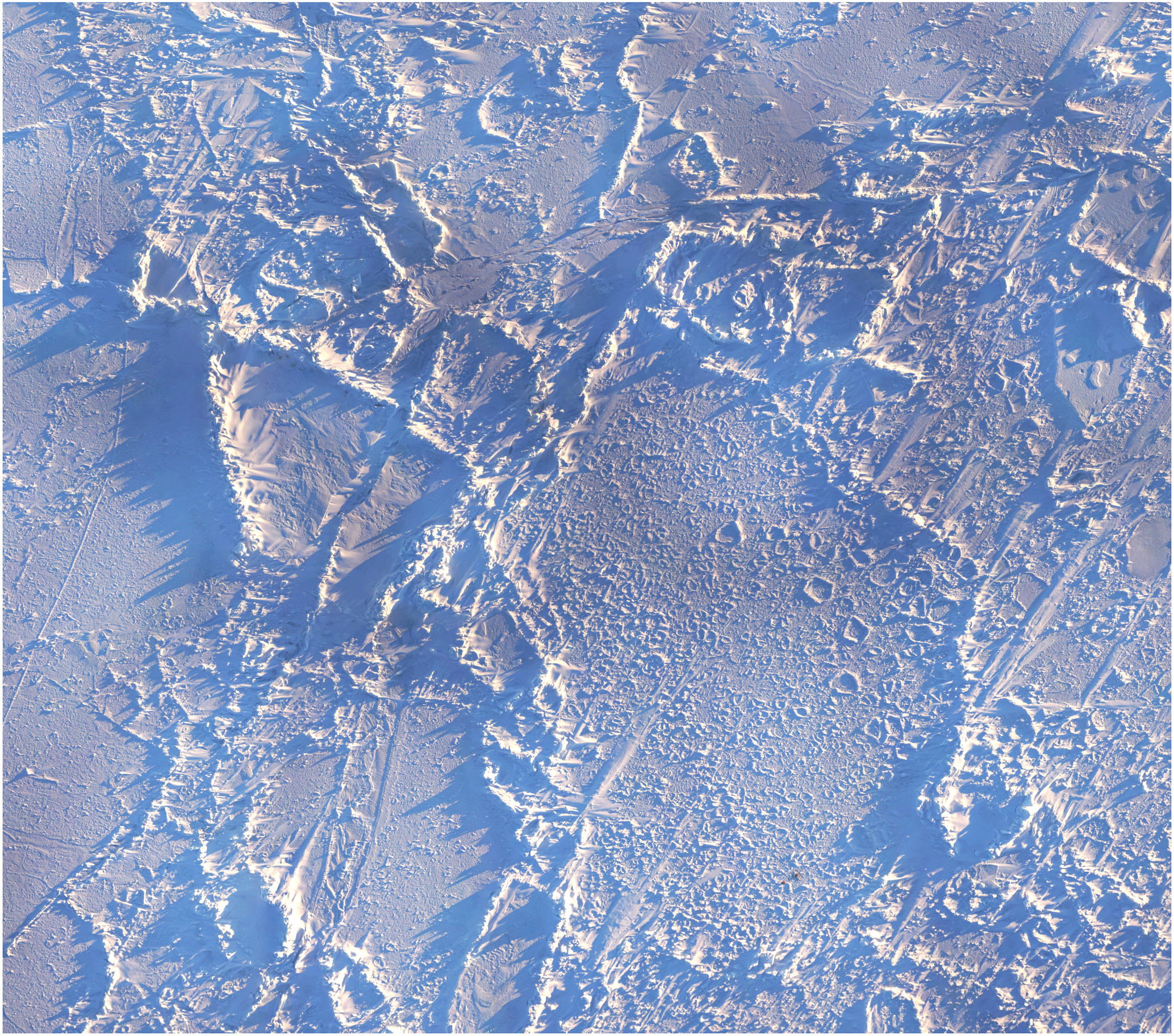
Figure 2Drone imagery (180 m × 180 m) of heavily deformed ice in the Ross Sea, Antarctica. There are multiple ridges, which cannot be easily separated. The ridge widths and slopes are varying and must be arbitrarily defined, leading to a variety of possible values. Image provided by Guy Williams.
The uncertainty in sea ice density is also a significant contributing factor to the high uncertainty of SIT estimates (Kern and Spreen, 2015). For example, if assuming zero ice freeboard (F=D in Eq. 1) with some known snow density, a 10 % uncertainty in the sea ice density can lead to a 50 % uncertainty in the SIT. As mentioned before, the effective density may also vary locally, particularly in deformed ice. On previous Antarctic fieldwork such as SIPEX-II in spring 2012, Hutchings et al. (2015) found the density of first-year ice in the presence of porous granular ice to be as low as 800 kg m−3, a difference of more than 10 % from the standard assumption of 900–920 kg m−3 (e.g., Worby et al., 2008; Xie et al., 2013; Maksym and Markus, 2008; Zwally et al., 2008; Timco and Weeks, 2010), but in line with the 750–900 kg m−3 range found by Urabe and Inoue (1988). This effective density could vary regionally and seasonally in line with ridging frequency, and knowing these variations with greater certainty would decrease the errors in SIT estimations. The effective density may also vary locally around areas of deformed ice, which have varying gap volumes. This means that the scatter in any given linear fit of T and F, and the variability between different fits for different datasets, can be interpreted as differences in effective densities; alternatively, this points out that linear fits will have an irreducible error due to local effective density variations.
In this paper, we aim to use a high-resolution dataset of deformed sea ice to develop better algorithms to estimate SIT from surface topography. Unlike previous studies which have relied on low-resolution, 2-D drilling transects, we use high-resolution, 3-D characterization of the snow surface from terrestrial lidar, coincident with 3-D ice draft from an autonomous underwater vehicle and detailed manually probed snow depth measurements. In particular, having 3-D coverage allows for the analysis of complex morphological features. First, we examine simple statistical relationships between snow freeboard, snow depth, and ice thickness and compare with prior studies. We also estimate densities of ice and snow by comparing the fits with Eq. (1) and compare with field data. Next, we use a deep-learning convolutional neural network to improve estimates of local ice thickness by using complex, nonlinear functions of 3-D surface morphology. Finally, we discuss the linear and convolutional neural network (ConvNet) models and attempt to interpret how learned features in the neural network may be related to physically meaningful morphological features, and we consider possible extensions to this work on larger datasets.
Our goal here is to test whether complex surface morphological information can be used to improve sea ice thickness estimation. In this paper, we demonstrate this using high-resolution spatial surface topography, which is most applicable to airborne remote sensing data such as those obtained by NASA's Operation IceBridge (Kurtz, 2013). While a somewhat different approach would be required for linear data such as those obtained from ICESat-2, this paper is a first test of proof of concept that using such information may be beneficial.
The PIPERS (Polynas, Ice Production and seasonal Evolution in the Ross Sea) expedition took place from early April to early June 2017 (Fig. 3). In total, six AUV ice draft surveys were taken of the undersides of deformed sea ice. Of these, four coincided with snow depth measurements and a lidar survey of the snow freeboard, thus providing a “layer cake” of snow depth, ice freeboard and ice draft data (following Williams et al., 2013). These four layer cakes are shown in Fig. 4. There are two other AUV scans which lack lidar and snow measurements so are not included in our analysis. The AUV surveys were carried out with a SeaBED-class AUV from the Woods Hole Oceanographic Institution following Williams et al. (2015), with a swath multibeam sonar (Imagenex 837 Delta T) at a depth of 15–20 m in a lawn-mower pattern (equally spaced passes under the ice in alternating directions). Adjacent passes were spaced to provide approximately 50 % overlap in consecutive swaths, with at least one pass across the grid in the transverse direction to allow corrections for sonar orientation in the stitching together of the final sonar map. The AUV multibeam data were processed to correct for vehicle pose, and then individual swaths were stitched together, with manual corrections to pitch and roll offsets of the sensors to minimize differences in drafts for overlapping portions of adjacent swaths. This largely follows the methodology in Williams et al. (2015), although simultaneous localization and mapping (SLAM) algorithms were not applied here as the quality of the multibeam maps were determined to be comparable to those without SLAM processing, and any improvements in resolving small-scale features would not affect the analysis here. The vertical error in draft is estimated at 10 cm over deformed areas and < 3 cm for level areas (Williams et al., 2015). The scans were ultimately binned at 0.2 m horizontal resolution. The snow freeboard scans were performed with a Riegl VZ-1000 terrestrial lidar scanner, using three to five scans from different sides of a 100 m × 100 m grid to minimize shadows, which were stitched together using tripod-mounted reflective targets placed around the grid. We scanned at the highest laser pulse repetition rate of 300 kHz, with an effective maximum range of 450 m. The accuracy and precision at this pulse rate are 8 and 5 mm, respectively. All composited and registered scans for a particular site were height-adjusted to a sea level datum using a minimum of three drill holes for sea level references. The output point cloud was binned at 0.2 m resolution, and any small shadows were interpolated over with natural neighbor interpolation (Sibson, 1981). The snow depth measurements were carried out last, using a Magnaprobe, a commercial probe by Snow-Hydro LLC with negligible vertical error when measuring snow depth on top of ice (Sturm and Holmgren, 2018; Eicken and Salganek, 2010). The probe penetrates the snow and automatically records the snow depth. It was fitted with an Emlid Reach real-time kinematic GPS, referenced to base stations on the floe, which allowed for more precise localization of snow depth. Using post-processed kinematic (PPK) techniques with the open-source RTKLIB library and correcting for floe displacement/rotation, the localization accuracy was ∼10 cm. The snow was sampled by walking back and forth in a lawn-mower pattern, with higher sampling clusters around deformed ice. A typical survey over the 100 m × 100 m area had ∼2000 points, with higher resolution (∼10 cm) near areas of deformed ice and lower resolution (∼5 m) over flat, level topography. These measurements were converted into a surface by using natural neighbor interpolation (Sibson, 1981), binned at 20 cm to match the lidar and AUV data. The ice thickness can then be calculated by taking (draft) + (snow freeboard) − (snow depth). Note that because of thin snow, a negligible portion of the ice had negative freeboard. Where they do tend to occur (in deeper snow adjacent to ridges), the effect on isostasy at the spatial scales considered here will also be negligible because of the much thicker ice.
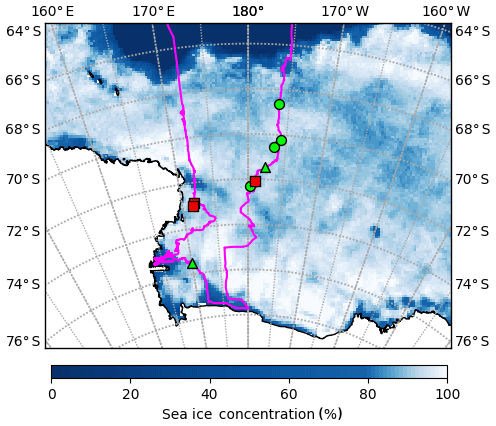
Figure 3PIPERS track (magenta) with locations of ice stations labeled. Stations with AUV scans are shown in green (3, 4, 6, 7, 8 and 9) and the other stations (1, 2 and 5) are shown with red squares. Stations 4, 7, 8 and 9 (green circles) also have a snow freeboard scan and snow depth measurements; these are shown in Fig. 4. Other stations have some combination of missing lidar, AUV and snow data. Station dates were 14 May for station 3, 24 May for station 4, 27 May for station 6, 29 May for station 7, 31 May for station 8 and 2 June for station 9. Overlain is the sea ice concentration data (5 d median) for 2 June 2017 from ASI-SSMI (Kaleschke et al., 2017).
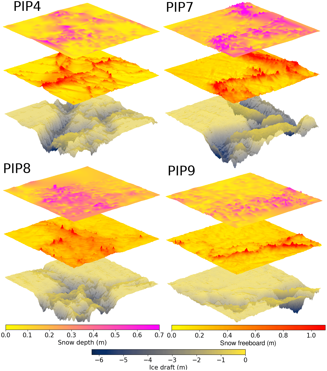
Figure 4Sea ice–snow layer cakes from PIPERS. The top layer is the snow depth (D), the middle layer is the lidar scan of the snow freeboard (F), and the bottom layer is the AUV scan of the ice draft. The ice thickness is therefore given by ice draft + snow freeboard − snow depth.
The lidar and AUV data were corrected with a constant offset, estimated by aligning with the mean measurements of the level areas of the drill line for each floe. It is important to use the level areas only as drill line measurements are likely to be biased low due to the difficulties of getting the drill on top of sails, potential small errors in alignment of the drilling line relative to the AUV survey, differences in thickness measurement in highly deformed areas (the drilling line samples at a point, while the AUV will be some average over the sonar footprint) and the presence of seawater-filled gaps that may be confused with the ice–ocean interface when drilling. The order of the lidar correction is ∼1 cm and the order of the AUV correction is ∼10 cm. This offset accounts for errors in estimating the sea level at lidar scan reference points and the AUV depth sensor and vehicle trim.
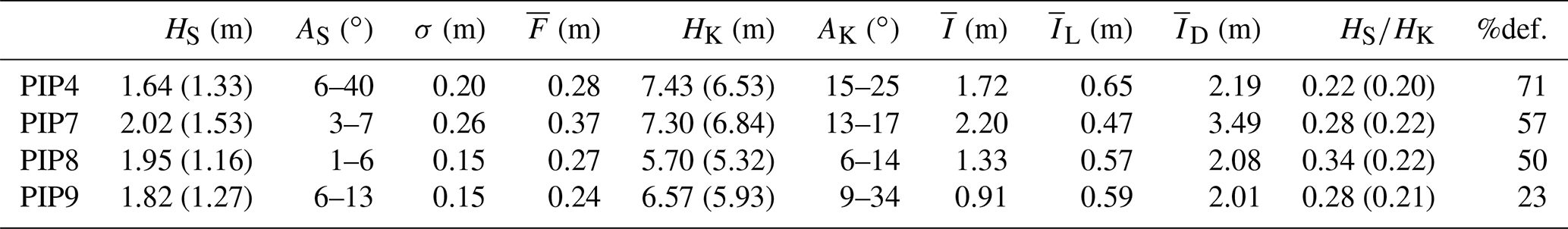
Summary statistics for the floes sampled during PIPERS are in Table 1. The PIPERS surveys comprised floes with ridges that had sails and keels significantly thicker than those that are typically sampled in drilling transects (e.g., Tin and Jeffries, 2003; Worby et al., 2008). The sail and keel angles (the angle of the sail and keel slopes relative to the vertical) are not as well-defined for complex, nonlinear ridges, so a range of angles are given, based on the variety of slopes measured across the deformed area. The 99th percentile for the sail and keel height is also reported to inhibit the effect of outliers from the lidar and AUV scans. We found the sail ∕ keel ratio was much more consistent when using the 99th percentile values. Our sail angles are typically < 10∘ and our keel angles are typically < 20∘, in line with averaged values from Tin and Jeffries (2003). However, our sail heights and keel depths are slightly larger in magnitude than the averaged Antarctic values from Tin and Jeffries (2003), and are more similar to their reported values for temperate Arctic ridges. Although our sampled ridges seem to be morphologically typical of Antarctic ridges, they are somewhat thicker than those typically sampled in drilling transects, which is consistent with Williams et al. (2015), who suggested that drilling transects may undersample thicker ice.
Table 1Standard metrics calculated for PIPERS dataset: sail height (HS), sail angle (AS), surface roughness (here taken as the standard deviation of the snow freeboard, σ), mean snow freeboard (), keel depth (HK), keel angle (AK), mean thickness (), mean level ice thickness (), mean deformed ice thickness (), sail-to-keel ratio (HS∕HK) and % deformation. For HS and HK, the absolute maximum is given, along with the 99th percentile value of the deformed section draft (in brackets). The amount of deformed ice in each scan is generally high as the survey grids were deliberately chosen for their deformation. The sail and keel angles are not precisely defined because the deformed surfaces are complex and nonlinear, and a range of slopes across the deformed surface are given.
3.1 Linear regression approach
We attempt to statistically model SIT using surface-measurable metrics (e.g., mean and standard deviation of the snow freeboard), in order to see the limitations of this method. To accurately calculate SIT without making assumptions of snow distribution, we need to use combined measurements of ice draft (AUV), snow freeboard (lidar) and snow depth (probe). Here, we primarily use PIPERS data to focus on early-winter Ross Sea floes and also because this is the largest such dataset from one season and region, which is important so that the ridges have consistent morphology.
We use a simple (multi)linear least-squares regression with either one (snow freeboard, F) or two (F and snow depth, D) variables with a constant term, such that .
For the two-variable fit, we do an additional fit with the constant forced to be zero, in order to obtain coefficients that can be used, following Eq. (1), to estimate the snow and ice densities.
To measure the fit accuracy, we use the mean relative error (MRE), as this avoids weighting errors from thin or thick ice differently. The value, adjusted for a different number of variables, is also reported where possible (it is not defined for a fit forced through the origin). When comparing the generalization of the fits to test data excluded from the fit data, we also report the relative error of predicting the mean survey-wide thickness (REM), as often researchers are interested in the aggregate statistics of a survey. These fit errors in estimating mean SIT are compared to both prior relationships derived from drilling data to highlight uncertainty when used with different ice conditions and to our ConvNet predictions of ice thickness.
In order to motivate more complex methods in subsequent sections, we also use surface roughness (standard deviation, σ) to predict thickness to demonstrate that surface morphological characteristics have some information that can be used to predict thickness.
3.2 Deep-learning approach
One advantage of deep-learning techniques is that they are able to learn complex relationships between the input variables and a desired output, even if the relationships are not obvious to a human. Although they are commonly used for image classification purposes, they can also be used for regression (e.g., Li and Chan, 2014). We expect a convolutional neural network (ConvNet) to achieve lower errors in estimating SIT, as they are able to learn complex structural metrics, in addition to simplistic roughness metrics like σ. Our input is a windowed lidar scan (snow freeboard) and an output of mean ice thickness. Notably, there is no input of snow depth, or any input of ice or snow densities. This allows the ConvNet to infer these parameters by itself and more importantly to potentially use different density values for different areas.
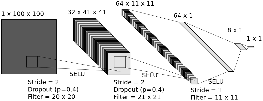
Figure 5ConvNet architecture, using three convolutional layers and two fully connected layers, for predicting the mean thickness (1×1 output) of a 20 m × 20 m (100×100 input) lidar scan window at 0.2 m resolution (LeNail, 2019). The 64×1 layer is made by reshaping the output of the final convolutional layer, and so is visually combined into one layer. The optimizer used was Adam with weight decay (Kingma and Ba, 2014). The initial learning rate was and reduced by a factor of 0.3 every 100 epochs until it reached .
Our architecture is shown in Fig. 5. The input consists of 20 m × 20 m (100 pixel × 100 pixel) windows, with three convolutional layers, with a stride of 2 in the first two layers, and two fully connected layers. We used scaled exponential linear units (SELUs) to create nonlinearity (Klambauer et al., 2017). The loss function used was the mean squared error. We also used dropout (p=0.4) and augmentation (random 90∘ rotations, horizontal and vertical flipping) to reduce overfitting (Srivastava et al., 2014). An overview of ConvNet basics and full implementation details are given in the Appendix.
The training–validation set consisted of randomly selected windows from three PIPERS ice stations, each on a different floe. We chose 20 m as the window size by using the range of the semivariogram for the floes (25 m), which we expect to represent the maximum feature length scale. This compares well to an average snow feature size of 23.3 m from early-winter Ross Sea drill lines from Sturm et al. (1998). We chose 20 m instead of 25 m windows to balance this with the need for a smaller window size to ensure a larger number of windows (data points) for our analysis. These data were randomly divided into 80 %–20 % to make the training and validation sets. The remaining floe (divided into windows) was kept as a test set, in case the training and validation windows had similar morphology and the validation set was thus not entirely independent of the training set. To prevent cherry-picking, the ConvNet was trained four times, with a different floe used as the test floe each time. Results are shown in Table 2. Although the training error is directly analogous to the fit error for linear models for some dataset, it is much easier to overfit with a ConvNet as the training error can be made arbitrarily low. As a result, we compare our validation error to the linear fit errors, and we also use our test errors as a test of the generalization of our model. From here onwards, analysis of the ConvNet refers to the one using PIP8 as a test set, though using a different one would yield qualitatively similar analysis.
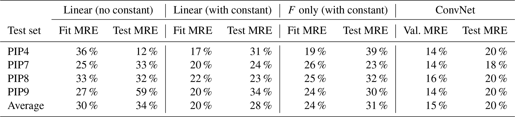
Table 2A compilation of the MRE of different fitting methods. Coefficients for the linear fits are shown in Table 3 and details are in Sect. 3.2.1–3.2.2. The leftmost column indicates the floe that was excluded from the fitting data (e.g., the first row indicates fits that were performed over the PIP7-9 data and then tested on PIP4). The ConvNet validation error was used for comparison with the linear model fits, as the training error can be made artificially low by overfitting. On average, the ConvNet achieves the best generalization in the fit, even though there are individual anomalous cases. For example, the F-only fit using PIP7 as a test set has a low test error than fit error, which simply means that the average snow ∕ ice ratio for PIP7 is similar to the averaged snow ∕ ice ratio for the other floes. The F-only fit is most comparable to our ConvNet as neither use the snow depth as an input.
4.1 Linear model results
4.1.1 Fitting to snow freeboard only
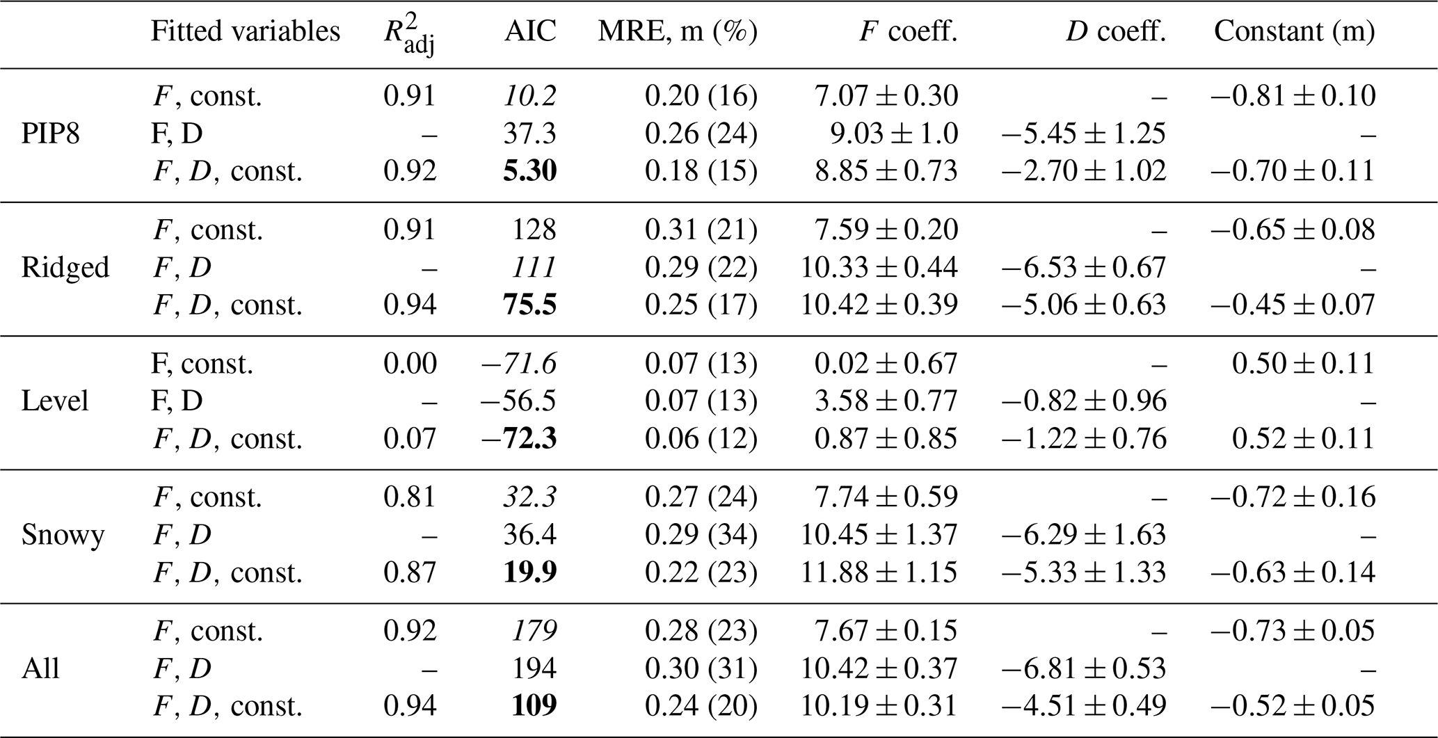
Although we have snow depth measurements in addition to snow freeboard measurements, in general there are far fewer snow data and so we first try to fit with just snow freeboard, by making some snow depth assumptions. This approach has been applied by Ozsoy-Cicek et al. (2013) and Xie et al. (2013) in order to obtain empirical relationships between SIT and snow freeboard. All our fitted coefficients are shown in Table 3. Because the R2 is not well-defined for a fit with no constant term, we can compare all the model fits with the AIC (Akaike information criterion, lower is better; see Akaike, 1974). For all categories except for “level”, the {F,D, constant} fit is indisputably best; for example, a difference in AIC of 70 between the two best models in the “all” category implies that the likelihood that the model with {F, constant} is better than the one with {F,D, constant} is . For the level category, the difference in AIC suggests that linear fits with {F,D, constant} and {F, constant} are very similar (the latter has a 50 % likelihood of being better than the former), which is consistent with the idea that level ice probably has a constant ice ∕ snow ratio such that introducing D as a variable does not improve much on using only F.
Table 3Fitted coefficients for SIT T as a multilinear regression of the snow freeboard F and snow depth D (Sect. 3.2.2), and also fitting for F only (Sect. 3.2.1). The variable “const.” refers to a constant term being included in the fit. Surfaces are also categorized (Fig. 7) to incorporate roughness into the fits (Sect. 4.1.3). As the R2 is not well-defined for a fit with no constant term, the Akaike information criterion (a metric that minimizes information loss) is used to compare the models (Akaike, 1974). The R2 is reported for the with-constant fits only and is adjusted for the different sample sizes in each fit. For each dataset, the smallest AIC value is bolded, and the second-lowest is italic. The absolute value of the AIC does not matter; only the relative differences between AICs for different models that use the same dataset matter, with the lowest being the best model. For individual floe fits, only PIP8 is shown for brevity as the other floes have comparable errors and coefficients.
Fitting gives a mean relative error (MRE) of 23 %. However, the slope is much higher (7.7), and the intercept is also larger and different in sign (−0.7 m) to existing fits in the literature (e.g., Ozsoy-Cicek et al., 2013, found that for an early-spring Ross Sea dataset). Using the fitted relationship from Ozsoy-Cicek et al. (2013) for our dataset, the MRE is 36 %, and the relative error in estimating the overall survey mean thickness (REM) is 41 %. This is perhaps partly due to the seasonal difference in these datasets, which itself implies that the proportion of deformed ice (and hence nonzero ice freeboard) is variable. Reasons for the difference in slope and intercept are given in Sect. 5.1.
We also test how well-generalized the fits are by fitting only three of our four surveys at a time, then testing the fitted coefficients on the remaining survey. These results are summarized in Table 2. The average fit error was 24 %, but the average test error was 31 %, which means that empirical fits to the snow freeboard may have errors of 31 % when applied to new datasets.
4.1.2 Fitting to snow freeboard and snow depth
For this section, we perform two different regressions: one with a constant and one without. The with-constant fit is intended to test whether introducing additional information improves the empirical fits, following Ozsoy-Cicek et al. (2013), and the without-constant fit is intended to be compared against Eq. (1) to estimate sea ice and snow densities. The coefficients are reported in Table 3 and the fit and test MREs are reported in Table 2. We can see that adding snow depth as a variable only slightly improves the fit MRE (average 20 %), but the fits remain poorly generalized, with a test MRE of 28 %, only slightly lower than the 31 % test MRE of fitting with F only.
Fitting without a constant allows us to directly compare the fitted coefficients with Eq. (1). Using typical values of 910 kg m−3 for ice density, 1027 kg m−3 for water density and 323 kg m−3 for snow density from Worby et al. (2011), the coefficients for the freeboard F and snow depth D should be 8.8 and 6.0. Similarly, Zwally et al. (2008) used corresponding densities of 915.1, 1023.9 and 300 kg m−3, giving a freeboard coefficient of 9.4 and a snow coefficient of 6.7. Our results when fitting over all four floes are 10.4 for c1 and 6.8 for c2, which are comparable to those inferred from Zwally et al. (2008), although there is considerable variation between the floes (7.9–10.6 for c1; 3.9–6.3 for c2; not shown in Table 3).
Assuming a density of seawater during PIPERS of 1028 kg m−3 (determined from surface salinity measurements at these stations), this gives bounds for the effective densities and standard errors of sea ice and snow as 929.4±3.5 and 356.3±57.2 kg m−3. The snow density is in line with Sturm et al. (1998), who found mean densities of 350 and 380 kg m−3 during autumn–early winter and winter–spring, respectively, in the Ross Sea, as well as the measured snow densities from PIPERS (245–300 kg m−3). The measured PIPERS snow densities may be biased low because they were measured at level areas and possibly do not represent snow densities in drifts around ridges well. The errors here are propagated from the standard errors found during the regression; they are therefore representative of the error in estimation of the mean densities over all data and do not represent actual ranges in the ice and snow densities. The ice (effective) density estimates here are averaged over the entire PIPERS dataset (including both deformed and undeformed ice) and thus may not apply to other samples from the Ross Sea in winter, as the effective density is affected by the proportion of ridged ice, which is deliberately overrepresented in our sample. Moreover, it is important to note that under this fitting method, the density estimates are coupled (due to ρi appearing in both coefficients in Eq. 1) and if the estimate of ρs decreases, ρi increases. For example, if ρi=935 kg m−3 (unusually, but not impossibly high for the effective density of ridged ice, which includes some proportion of seawater – see Timco and Frederking, 1996), the best estimate for ρs becomes 312 kg m−3, which is closer to the measured 300 kg m−3 value from PIPERS.
The fact that introducing snow depth as a variable only slightly improves the generalization of the fit may be because snow depth is itself highly correlated with snow freeboard Ozsoy-Cicek et al. (e.g., 2013). Linear methods of fitting require the assumption of a constant snow and ice density (or in a one-layer case, a constant “effective density”), which implies an irreducible error for estimating small-scale SIT. This fails to account for varying ice and snow densities around level and deformed ice. This is discussed further in Sect. 5.1, and motivates the introduction of surface roughness (σ) as an additional variable in our linear fit.
4.1.3 Incorporating surface roughness into the fit
Given that we expect effective density variations for different surface types, we expect SIT estimates to improve with the addition of surface morphology information. The most simple of these is the surface standard deviation, as prior studies have found that this is correlated to the snow depth and the mean thickness (Kwok and Maksym, 2014; Tin and Jeffries, 2001). Our data also show a reasonable relationship between SIT and surface σ, though it is weaker than fits to the freeboard (Fig. 6). Adding the roughness as a third variable to the fit gives an average fit MRE of 18 % and an average test MRE of 24 %. This is not much of an improvement, and it is possible that σ is too simplistic a metric to improve the fit or that it is itself highly correlated with F and therefore offers little additional information.
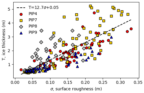
Figure 6Predicting mean ice thickness with just the surface roughness (σ) as the input, with MRE 33 %. The best-fit line is also shown, with R2=0.65.
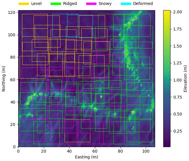
Figure 7An example lidar scan from a station (PIP7) with the manually classified segments. Snow features are clearly visible emanating from the L-shaped deformation. Deformed (blue) surfaces were excluded from the analysis.
There is no particular reason to expect the surface σ to be linearly combined with the snow depth and snow freeboard, even if it makes dimensional sense. Instead, we can try using the roughness as a regime selector. To do this, the lidar windows were classified manually into snowy surface, level surface, ridged surface and deformed surface categories (Fig. 7). If it had both a ridge and snow, it was classified as ridged. “Level” surfaces were distinguished as those windows with no visible snow or ice features in the majority of the window. “Snowy” surfaces were those that contained a snow feature (e.g., a dune or drift) in the window. “Deformed” was intended as a transitional category for images that had no clear ridge but were generally rough – this comprised, typically, ∼5 % of an image and was excluded from analysis. We acknowledge that this classification can be arbitrary, and we use this method only to show that different surface types should be treated differently, but a manual classification does not help much: this motivates the use of a deep neural network in the next section. The snowy, level and ridged categories were individually fitted to see if there were any differences in the coefficients; these are also reported in Table 3.
We then used a two-regime model over all four floes, so that ice thicknesses for the low-roughness surfaces are estimated using the level coefficients, and high-roughness surfaces use the ridged coefficients. This resulted in MREs of 16 %–21 % assuming 20 %–50 % of the surface is deformed. This is slightly better than for fitting the all category in Table 3 (20 % MRE), suggesting that distinguishing topographic regimes improves thickness estimates. However, this fit has issues with generalizing to other floes. If the fit for the rough and level coefficients is carried out using only three floes and then applied to the remaining (test) floe (using a surface roughness threshold determined from that floe, and again assuming 20 %–50 % of the surface is deformed), the test MREs averaged over all possible choices of test floe are considerably higher (24 % when fitting). This does not improve much on the generalization from the two-variable linear fit, where the test MRE was 28 %.
4.2 ConvNet results
The (irreducibly) poor generalization of linear fits, likely due to a locally varying proportion of snow and ice amongst different surface types, motivates the use of more complex algorithms that can account for the surface structure. For this, we use a ConvNet with training, validation and test datasets as described in Sect. 3.2.
The best validation error was 15 %, corresponding to a training error of 11 % (Fig. 8a and b). The mean test error (on the excluded floe) was 20 %. Although the linear models have a similar fit error, they do not generalize as well to the test set, and the resulting thickness distribution is visibly different to the real test distribution (Fig. 8c).
This shows better generalization than the linear models (test MREs from 28 % to 47 %). Although the best-performing linear models have only slightly higher test MREs (24 % for the three-variable fit in Sect. 4.1.3) than our ConvNet (20 %), the range of errors is much greater, with test MREs of 18 %–29 %, whereas the ConvNet has remarkably consistent test MREs of 18 %–20 %. Furthermore, it is important to remember that achieving these comparably low MREs with linear models requires snow depth as a variable, which is generally not available. These fits also typically include a negative constant (Table 3), which means T < 0 for , which is clearly unphysical and limits the application of these models to areas of low snow freeboard. The fits to snow freeboard only, which uses the same input data as the ConvNet, have considerably higher test MREs (23 %–39 %; see Table 2). For the sake of comparison to models that use rms error, such as Ozsoy-Cicek et al. (2013), the validation rms error for our survey-averaged mean thickness values is 2 cm, which is lower than the rms error of 11–15 cm from Ozsoy-Cicek et al. (2013). Our fit uses three surveys from three different floes as an input, which means the fit is likely lower in error than Ozsoy-Cicek et al. (2013), which uses 23 floes. However, we would also expect poorer generalization for our test set from using only three surveys. Although our test rms error for the mean survey thickness (3 cm) cannot be directly compared, it is reasonable to surmise that our ConvNet achieves better generalization than a linear fit. Note that the rms error is not linked to the surface rms roughness, which is just the standard deviation of the snow freeboard.
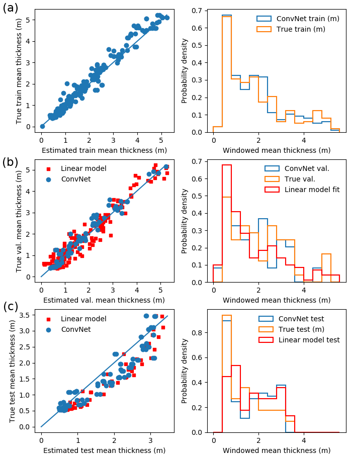
Figure 8ConvNet results, with (a) the learned ConvNet model applied to the training data (80 % of randomly sampled 20 m × 20 m windows from PIP4, PIP7, PIP9), with MRE 12 %; (b) the learned ConvNet model applied to the validation data (remaining 20 % of the randomly sampled 20 m × 20 m windows from PIP4, PIP7 and PIP9) with a MRE of 16 % as well as a linear model (with snow freeboard + constant) fitted to PIP4, PIP7 and PIP9 with a MRE of 25 %; (c) the learned ConvNet model and fitted linear model applied to randomly sampled 20 m × 20 m windows from PIP8, as a check against learning self-similarity, with MREs of 20 % (ConvNet) and 32 % (linear model)). In each case, the left panel shows a scatter plot with the predicted and true thicknesses, and the right panel shows the resulting thickness distribution. Our results suggest slight overfitting, as the test error is higher than the training error, but the learned model still generalizes fairly well, with MREs much lower than linear models, even when including an unphysical intercept to improve the fit (Table 2).
As shown in Fig. 8c, the ConvNet does seem to be capturing the thickness distribution of the test floe, even if the individual window mean estimates have some scatter. In contrast, the linear models have considerably different thickness distributions (Fig. 8, red points and lines) despite having similar fit MREs (Table 2). The ConvNet also successfully reproduces the spatial variability of the SIT distribution better than the linear fit (Fig. 9). Note because of the small size of the dataset, there is significant oversampling in the ConvNet prediction of the floe SIT distribution. The primary difference between the ConvNet and linear fit for this floe is a large overestimation of level ice thickness. This demonstrates the inability of the linear fit to account for variations in effective densities and/or snow ∕ ice freeboard ratios. The ConvNet prediction can have some large local errors, in this case chiefly on the flanks of the ridge, where steep freeboard or thickness gradients may affect performance. Comparisons for other floes (not shown) are qualitatively similar, though the spatial distribution of fit errors varies among floes. The key result of the ConvNet is in the significantly reduced error in the local (20 m scale) mean thickness (MRE of 15 %–20 %), which also gives a low ∼10 % error of the average scan-wide thickness. Moreover, this high accuracy also carries over to test sets from the same region and season. In contrast, linear models, which do not generalize well to new datasets, have a considerable bias (Fig. 9), despite having an ostensibly good fit. Analysis of why the ConvNet may be performing better than linear fits is given in Sect. 5.2.
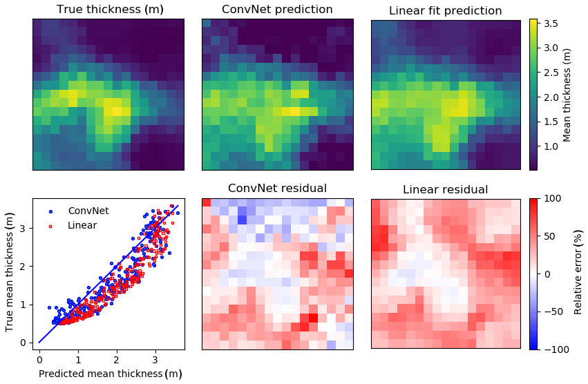
Figure 9Ice thickness profile of the test set (PIP8), using the linear fit () and ConvNet model, both performed with PIP4, PIP7 and PIP9 as inputs. The input windows are 20 m × 20 m, with a stride of 5 m in each direction, so there is a considerable oversampling. The mean residual for the linear model (35 cm) is much higher than for the ConvNet (19 cm), which means the resulting mean thickness has almost twice the REM (24 % vs. 13 %). The scatterplot clearly shows the linear model (using 20 m windows as well, with coefficients from Table 3) predictions are consistently biased high, which is also apparent in the linear model residual.
5.1 Possible causes for poor linear fit
Our linear regression results for fitting have markedly different coefficients from drill line data from the same region and season (Ozsoy-Cicek et al., 2013). Here we discuss possible reasons for their differences. The first difference is that our value for c1=7.67 (Table 3) is much higher. This is almost certainly because our dataset includes much more deformed ice, as we deliberately sampled deformed areas on floes. At one extreme, where the snow load is large such that the snow depth = snow freeboard assumption is approximately valid (set F=D in Eq. 1), which for our data occurs for level, thin ice where there is some snow load, Eq. (1) would simplify to T=2.7F (using density values from Zwally et al., 2008). In contrast, when the topography is sufficiently rough, there is considerable ice freeboard, which may even exceed snow depth. If we assume the snow is negligible (D=0), which may be the case at the sail peak, Eq. (1) becomes T=9.4F. These values become lower and upper bounds for fitting c1 in T=c1F (without the constant c0). The best fit value for c1 is 5.8 when fitting to the full dataset (Fig. 10), which falls between these two extremes of snow-only F and ice-only freeboard F. Our coefficient is also comparable to Goebell (2011), who found a coefficient of 5.23 from first-year Weddell ice. Much as in Goebell (2011), our dataset includes considerable deformed ice, which has a nonzero ice freeboard, and so the coefficient of F is higher than 2.7. We can estimate the ratio of snow to ice by comparing this with the hydrostatic equation: for example, if we assume typical snow and ice densities of 300 kg m−3 and 920 kg m−3, this implies that snow, on average, comprises 54 % of the measured snow freeboard. Using these values, Eq. 1 simplifies to T=5.8F, as in Fig. 10. In further support of this, our dataset has mean snow depths for the four surveys ranging from 16 to 26 cm and mean snow freeboards ranging from 24 to 37 cm, implying considerable nonzero mean ice freeboards.
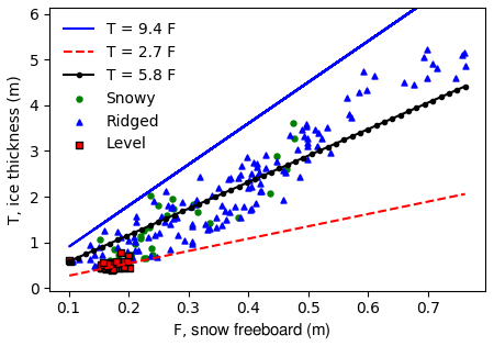
Figure 10The SIT (T) as a function of measured snow freeboard (F). As expected, all points lie between the two extreme regimes (no ice freeboard and no snow freeboard). The level surfaces mostly have no ice freeboard, as expected, though there is some scatter that suggests a varying component of ice freeboard. The best-fit line for all windows from Table 3 is shown in black. Assuming mean snow and ice densities of 300 and 920 kg m−3, this implies a mean proportion of 55 % snow and 45 % ice in the snow freeboard. Again, the scatter around the best-fit line indicates that this proportion is changing. Some points for the level category fall below the T=2.7F line, suggesting that snow densities in these areas are <300 kg m−3 (or effective ice density < 915 kg m−3.)
The high scatter of our fit also suggests that the snow ∕ ice ratio varies locally, as can be expected around level and deformed ice. If the proportion of ice to snow were constant, then the best-fit line, for whatever slope, would have no scatter. This is not the case in Fig. 10, and indeed the standard deviation of ice freeboard across all windows was 7.9 cm (mean: 9.0 cm). This means that assuming a constant snow and ice density or a constant snow–ice proportion is not justified, and hence it is likely that simple statistical models break down when looking at deformation on a small scale or when large-scale snow deposition and ice development conditions vary. This mirrors the conclusions in Kern et al. (2016), who found that linear regressions could not capture locally and regionally varying snow ∕ ice proportions. Even when including regime-dependent fits (Sect. 4.1.3, Fig. 6), this does not improve the test errors because this is likely too simplistic (even within a ridge, the ratio of snow to ice is likely varying). An important point regarding σ is that it does not actually account for the surface morphology very well, as any permutation of elevations within the window will give the same σ. This means that the “shape” or “structure” of the surface is not truly accounted for. This motivates more complex metrics for surface roughness (Sect. 4.2).
Unlike our approach, the fits in Ozsoy-Cicek et al. (2013) and Xie et al. (2011) use large-scale, survey-averaged data. Their coefficients for c1, 2.4–3.5 and 2.8 for Ross Sea and Bellingshausen Sea data, respectively, are near the theoretical value of 2.7 assuming no ice freeboard. This suggests that at large scales for some seasons and regions, it may be reasonable to assume that the mean ice freeboard is zero, but this is not the case at smaller scales. It is also possible that drill lines have undersampled ridged ice due to sampling constraints or (in our case) sample heavily deformed areas that are not typically sampled in situ. Thus, empirical fits should be used with caution.
The second major difference is that our intercept is negative, whereas those from Ozsoy-Cicek et al. (2013) and Xie et al. (2011) are all positive. In our case, it is possible to interpret our negative intercept as a result of fitting a linear model across two roughness regimes. From above, the two regime extremes (no-ice vs. no-snow contribution to snow freeboard) give T=2.7F and T=9.4F as limiting cases. In general, we expect the proportion of ice freeboard to gradually increase as F increases from thinner, level ice to thicker, deformed ice. Although snow also accumulates around deformed ice, there may also be local windows at parts of the ridge with no snow (e.g., the sail). This means that we expect a gradual transition from T=2.7F to T=9.4F as F increases. Fitting one line through these two clusters of points would result in a coefficient for F between 2.7 and 9.4 and a negative intercept, which we find in almost all our cases. The one exception is the fit for the level category, which is essentially a null fit (as over 90 % of the thickness values are clustered around 0.5±0.05 m). In contrast, the coefficients for F from Ozsoy-Cicek et al. (2013) and Xie et al. (2011) are all ∼3 because these studies average over multiple floes and have a sufficiently small proportion of deformed surface area to assume a negligible ice freeboard as discussed above. In their case, their intercept would be positive, as their ice thickness estimates would be otherwise underestimated due to some of the snow freeboard being ice instead of snow.
When fitting a linear or ConvNet model to snow freeboard data, we cannot know whether there are negative ice freeboards; as such, these methods account for it only implicitly, with a linear fit effectively assuming that a similar percentage of freeboards will be negative. This may contribute to errors when trying to apply a specific linear fit to a new dataset. A ConvNet could conceivably do better here, in that significant negative freeboard is likely to matter most when there is deep snow, which might have recognizable surface morphology, although this is quite speculative.
5.2 Plausible physical sources of learned ConvNet metrics
The ConvNet performs better than the best linear models in both fit and test MREs. However, the ConvNet trained with our dataset is very limited in applicability to only datasets from the same region and season. When we applied our trained ConvNet to lidar inputs from a different expedition (SIPEX-II; Maksym et al., 2019) from a different season and region, the MRE is 69 %, and the REM is 51 %. This suggests that other seasons and regions may have different relationships between the surface morphology and SIT, which is not surprising given that snow accumulates throughout winter. The SIPEX-II data were collected during spring in coastal East Antarctica in an area of very thick, late-season ice with very deep snow with large snowdrift features of length scales > 20 m (which would not be resolved by the ConvNet filters here). It is also possible that datasets from spring, such as SIPEX-II, will not be as easy to train networks on because the significantly higher amounts of snow may obscure the deformed surface. Although this points out a limitation of this method, which restricts any trained ConvNet to a narrow temporal–spatial range, it also adds weight to the idea that the ConvNet is learning relevant morphological features. A ConvNet trained on Arctic data would likely learn different features (e.g., melt ponds and hummocks), although additional filters may be needed to distinguish multiyear and first-year floes.
We also tried different inputs, such as using 10 m × 10 m windows, which had training, validation, and test errors of 9 %, 18 %, and 25 % and using 20 m × 20 m inputs with half the resolution (i.e., 0.4 m), which had errors of 7 %, 13 % and 25 %. The smaller window case has a slightly higher validation error than the above ConvNet, and the coarser-resolution input has a slightly lower validation error than the above ConvNet, but both cases have slightly higher test errors. Larger windows, which are more likely to capture surface features, are likely to improve the fit, but our dataset is too small to test this as larger window sizes would mean fewer training inputs. However, it is promising that the validation errors are lower at a coarser resolution. This suggests that this method may indeed extend to coarser, larger datasets like those from airborne laser altimetry from OIB. We also tried training for the mean snow depth given the lidar inputs, with training, validation, and test errors of 15 %, 17 % and 18 %, which is very similar to the thickness prediction. This is not entirely surprising as, if hydrostatic balance is valid, being able to predict the mean thickness given some snow freeboard measurements naturally gives the mean snow depth via Eq. (1).
Although the ConvNet achieved a much lower test error than the linear fits, the inner workings of a ConvNet are not as clear to interpret. We can try to analyze the learned features by passing the full set of lidar windows through the ConvNet to see if the final layer activations resemble any kind of metric. The below analysis of features is very qualitative, as it is inherently very difficult to characterize what a ConvNet is learning.
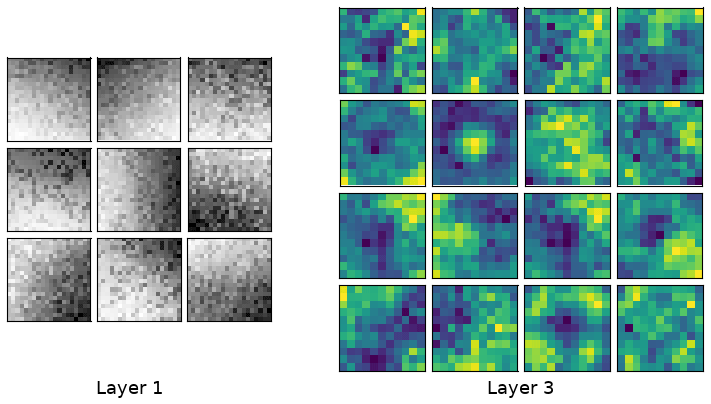
Figure 11Typical weights learned in the first and last convolutional layers. Weights learned from the third layer are shown using the same color map as the snow freeboard in Fig. 7 to facilitate comparison. Darker colors indicate lower weights, but the actual values are not important. The filters in layer 1 correspond to edge detectors, e.g., Sobel filters, and the filters in layer 3 may be higher-order morphological features like “bumps” (snow dunes) and linear, strand-like features (ridges). The filter size of the first layer corresponds to 4.0 m (20 pixels at 0.2 m resolution) and the third layer is 8.8 m (11 pixels at 0.8 m resolution). The resolution is halved at each layer due to the stride of 2 (see Fig. 5).
One helpful way to gain insight into what the ConvNet is learning is to inspect the filters. Filters in early layers tend to detect basic features like edges (analogous to a Gabor filter, for example), with later layers corresponding to more complex features like lines, shapes or objects (Zeiler and Fergus, 2014). We see similar behavior in our filters; typical filters learned in our model are shown in Fig. 11. Early filters highlight basic features like edges when convolved with the input array, while later filters show more complex features. These complex features are hard to interpret, but are clearly converged and not just random arrays. For example, a “blob” feature could be a snow dune filter, while filters with a clear linear gradient could correspond to the edge of ridges. The filters in the final layer are around ∼8 m in size. This may be too small to resolve the entire width of the ridges in our dataset, but would be enough to identify areas near ridges. With a larger windowed lidar scan, such as those from OIB with a scan width ∼250 m (Yi et al., 2015), we expect better feature identification, as the entire width of a ridge can be resolved within a filter.
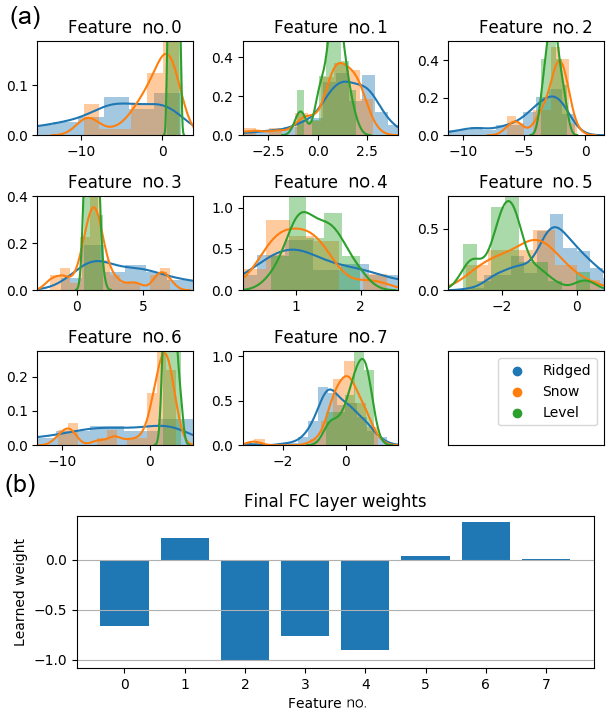
Figure 12(a) Distribution of the final (8×1) layer activations for the level, ridged and snow categories from Fig. 7, and (b) the learned weights for the final fully connected hidden layer. To generate the final thickness estimate, the activations in (a) are multiplied with the weights in (b) and then summed.
The learned weights for the final (8×1) hidden layer and their activations (when each input window is fed forward through the ConvNet) are shown in Fig. 12a, grouped by category (level, ridged, snowy). These should correspond to (unspecified) metrics, which are linearly combined with the weights shown in Fig. 12b. It is clear that level surfaces are distinguished from ridged and snowy surfaces, but ridged and snowy surfaces show considerable overlap with each other. While it is not possible to determine with full certainty what each of the eight features corresponds to, we can correlate these features to metrics that we may expect to be important for estimating the ice thickness and see which ones match. Performing this analysis, for ridged surfaces, features 0, 3 and 6 had a strong correlation () to the mean snow freeboard (Fig. 13d); for snowy surfaces, these three features had a slightly weaker correlation () to the mean snow freeboard; and for level surfaces, features 1 and 5 had a slight correlation ( and 0.80, respectively) to the mean snow freeboard (Fig. 13a). However, features that correlated to the ridged surface mean snow freeboard did not correlate to the level surface mean snow freeboard, and vice versa (Fig. 13b and c). This suggests that the mean snow freeboard for level surfaces is treated differently (e.g., given a different effective density) than other categories.
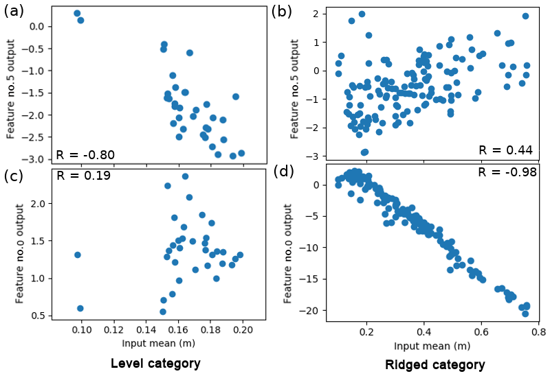
Figure 13Scatter plot showing correlations between features and real-life metrics. Here, features 0 and 5 correlate strongly to the mean elevations of the level and ridged surfaces, respectively, but not the other way around. This suggests that the level and ridged surfaces are treated differently, implying a different effective density of the surface freeboard. The correlation for the level category is not as strong; without the two points near x=0.1, , so this feature is possibly a combination of the mean elevation and something else.
For ridged surfaces, in addition to the mean snow freeboard, the rms roughness was also important, with features 2 and 4 weakly correlating () to the standard deviation of the window. The standard deviation had a slightly weaker correlation () for level surfaces and virtually none at all for snowy surfaces (). Another measure of roughness is the rugosity (the ratio of “true” surface area over geometric surface area; see Brock et al., 2004). This was most important for the snowy category, with for feature 7, compared to for feature 6 for ridged surfaces and for feature 2 for level surfaces. As we found before, these features were much more strongly correlated to the mean elevation and standard deviation, respectively for their respective surface category. This was not the case for feature 7 for snowy surfaces, which had a similar correlation () to the mean elevation and a much weaker correlation () to the surface σ. To summarize, for all categories, the mean snow freeboard is important (though weighted differently, as different filters activate for different categories). For both level and ridged surfaces, the rms roughness is important, and for snowy surfaces, the rugosity is also important. The above analysis suggests that there are important regime differences for estimating SIT. It should be noted that these statistical metrics suggested above, with the exception of rugosity, do not account for structure (any permutation of the same numbers has the same mean/σ), which limits the usefulness of this approach to interpreting the ConvNet.
This is by no means an exhaustive list, but it suggests that the ConvNet is learning useful differences between different surface types. However, as suggested by the considerable overlap in the distributions in Fig. 8, these categories may also not be the most relevant classifications. Alternatively, a t-distributed stochastic neighbor embedding (see van der Maaten and Hinton, 2008), which is an effective cluster visualization tool, shows that ridged and level surfaces are clearly distinguishable, but there is considerable overlap between the snowy and ridged categories (Fig. 14). However, the ridged category is quite dispersed, and may even consist of different classes of deformation which should not be grouped all together. Nevertheless, it is apparent that at the very least, the level and non-level categories are meaningfully distinguished. With more data and larger scan sizes (e.g., from OIB), a deep-learning neural network suitable for unsupervised clustering (e.g., an auto-encoder) could identify natural clusterings with their associated features (Baldi, 2012).
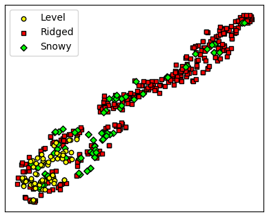
Figure 14The t-distributed stochastic neighbor embedding diagram for the encoded input, using the first fully connected layer (feature vector of size 64) (van der Maaten and Hinton, 2008). The level and ridged categories are most clearly clustered, although the snowy category may also be a cluster. There is some overlap between the snowy and ridged clusters, which may reflect how ridges are often alongside snow features. It is also possible that the ridged category contains multiple different clusters. This result suggests that the manually determined surface categories shown in Figs. 7 and 12 are pertinent, but perhaps not the most relevant, for estimating SIT given different surface conditions.
To emphasize the importance of the mean elevation, we also tried training the same ConvNet architecture with demeaned elevation as the input. Our ConvNet architecture is able to achieve a lowest validation error of 25 % (training error 10 %), but the test MRE is relatively high (40 %). The test error is worse than the linear model and has twice the test MRE of our ConvNet with snow freeboard (test MRE: 20 %).
We also trained the ConvNet to predict the mean snow depth, with comparable training, validation, and test errors of 15 %, 17 %, and 18 % when using raw lidar input and errors of 15 %, 22 %, and 45 % when using demeaned lidar input, which suggests the same analyses hold for snow depth prediction. As the snow depth is largely correlated with the snow freeboard (e.g., Ozsoy-Cicek et al., 2013), with the exception of ridged areas, it is not surprising that the demeaned input is not as good a predictor of the snow depth. However, when metrics obtained from the demeaned snow freeboard (such as roughness) are combined with the mean snow freeboard, snow depth estimates (as well as SIT estimates) are improved. This may mean that aside from the mean snow freeboard, surface lidar scans may contain other information (e.g., morphology) capable of improving both SIT and snow depth predictions. This is promising for applications to larger datasets such as OIB or ICESat-2.
Another approach to analyze these learned weights is to look at the sign of the weight and the typical values of the activations in Fig. 12. Feature 0 has a negative weight for which the ridged category (and to a lesser extent snowy) has the largest (most negative) feature values; this leads to adding extra thickness, primarily for the ridged ice category. This perhaps accounts for a higher percentage of ice freeboard in the snow freeboard measurement than for the level and snowy categories. Indeed, most of the level category has values near 0 for this feature. This could therefore be interpreted as a “deformation correction” of some sort, or increasing the effective density of the ridged surface (perhaps due to a higher proportion of ice). This is also the case for features 3 and 6, which is not surprising as these three features all had strong correlations to the mean elevation for the ridged and snowy categories.
Features 5 and 7 both show some distinguishing of the different surface types, although the weights are so small for these features (Fig. 12b) that they likely do not significantly change the SIT estimate and we do not speculate what these may account for.
The inner workings of ConvNets are not easily interpreted, but the analysis here suggests that the ConvNet responds in physically realistic ways to the surface morphology. It may be possible to use these physical metrics to construct an analytical approximation to the model, but due to the nonlinearities in the ConvNet as well as the considerable scatter between the features and our guessed metrics, this will not be as accurate as simply passing the input through the ConvNet.
Statistical models for SIT estimation suffer from a lack of generalization when applied to new datasets, leading to high relative errors of up to 50 %. This is problematic if attempting to detect interannual variability or trends in ice thickness for a region. Deep-learning techniques offer considerably improved accuracy and generalization in estimating Antarctic SIT with comparable morphology. Our ConvNet has comparable accuracy to a linear fit (15 % MRE vs. 20 % MRE) but it has much better generalization to a test floe (20 % MRE vs. 28 % MRE for applying the best linear fit). This linear fit uses additional snow depth data not included in the ConvNet; without these data, the linear fit has an even higher test MRE of 31 %.
We find that even for level surfaces, there is a considerable varying ice freeboard component that creates an irreducible error in simple statistical models, but can be accommodated as a morphological feature in a ConvNet. Our error in estimating the local SIT is < 20 % (rms error of ∼7 cm) and the resulting mean survey-wide SIT also has lower errors (rms error: 2–3 cm) than empirical methods (11–15 cm; see Ozsoy-Cicek et al., 2013).
In applying any model to a new dataset, it is assumed that the relationships from the fitted dataset hold for the new dataset. We already showed that linear fits do not hold for different datasets (even from the same region or season), with the MRE increasing substantially, likely due to differing snow–ice proportions in the snow freeboard. This is true even when applying relationships from some PIPERS floes to other PIPERS floes. In addition to different surveys having different freeboards, ice–snow densities may also be differently distributed between surveys. Our ConvNet has errors of 12 %–20 % when estimating both the local and survey-wide thicknesses of a test dataset, which is only slightly higher than the validation errors of 7 %–15 %. This suggests that the morphological relationships learned in the ConvNet also hold for other floes of comparable climatology, which in turn suggests that deformation morphology may be consistent within the same region and season.
Although our survey consists of high-resolution lidar, snow and AUV data, we really only need high-resolution lidar data. Lidar surveys are much easier to conduct than AUV surveys, and so a viable method for obtaining more data for future studies is to use a high-resolution lidar scan, combined with coarser measurements of mean SIT (e.g., with electromagnetic methods, as in Haas, 1998). Snow depth measurements are not needed with this method. This should greatly reduce the logistical difficulties to extend these methods to more regions and seasons.
Another possible strength of our proposed ConvNet is that it could account for a varying ice and snow density, with greater complexity and accuracy than an empirical, regime-based method. Although recent works like Li et al. (2018) have attempted to vary effective surface densities using empirical fits, these are not effective at higher resolutions, where snow and ice proportions may vary locally. Although the workings of ConvNets are somewhat opaque, we have shown that our ConvNet takes into account the spatial structures of the deformation, and given plausible justifications for why the snowy, level and ridged surfaces are treated differently. The learned filters suggest that morphological elements are important for SIT estimation.
Although our ConvNet would be greatly improved with more training data, it is promising that local SIT can be accurately predicted given only snow freeboard measurements. More extensive lidar, AUV and snow measurements from different regions and seasons would improve the ConvNet generalization. The window size of 20 m × 20 m used here may also be valid, with some modifications, to work on OIB lidar data, as the learned features at ∼8 m resolution are also resolved by OIB lidar data (resolution 1–3 m).
We have shown that surface morphological information can be used to improve prediction of sea ice thickness using machine learning techniques. This provides a proof of concept for exploring such techniques to similarly improve sea ice thickness prediction (particularly at smaller scales) for airborne or satellite datasets of snow surface topography. While the ConvNet technique presented here is not directly applicable to linear lidar data such as from ICESat-2, related methods that exploit sea ice morphological information might help improve sea ice thickness retrieval at smaller scales from ICESat-2. Alternatively, using a larger training set, it may be possible to use deep-learning-based methods to more readily identify relevant metrics for predicting SIT that may be measured/inferred from low-resolution, coarser data like ICESat-2 or Operation IceBridge.
The PIPERS layer cake data used here are available at https://doi.org/10.15784/601207 (Jeffrey Mei et al., 2019) and https://doi.org/10.15784/601192 (Stammerjohn, 2019) .
For a comprehensive introduction to deep learning, the reader is directed to Shalev-Shwartz and Ben-David (2014). Here we will give the details of our ConvNet and explain the importance of chosen parameters.
Convolutional neural networks, commonly known as ConvNets, are a class of deep neural networks that convolve filters (matrices that contain weighting coefficients, or weights) through the input array. The input array is typically an image, and the learned filters typically correspond to basic edge detections in initial layers and more complex features in later layers (e.g., Krizhevsky et al., 2012). Here, we use the lidar elevation scan as an input, due to its similarity to a grayscale image.
Like other deep-learning methods, ConvNets “learn” by updating their weights. This is done through comparing the output of the prediction with the true output, using the derivative of a loss function (here, mean squared error) propagated through the layers in reverse (backpropagation). The weight update rule, in its most basic form, is , for some weight w, loss function E and learning rate η. The value of η is important to ensure convergence: too high, and the filters may not converge (and may even diverge); too low, and the filters may take too long to converge. In order to introduce nonlinearities in the network, a nonlinear activation function is used at each layer. Typically, this is done with a rectified linear unit (ReLU), which zeros out all negative activations. We chose a scaled exponential linear unit (SELU), which has been found to improve convergence (Klambauer et al., 2017), as ReLUs sometimes lead to dead weights when dealing with many negative values. As convolutions by default shift by 1 pixel at a time, this leads to considerable overlap and large output sizes at each layer. To combat this, the filters can shift by a different number; this is called the stride.
ConvNets are normally used in image classification problems due to their ability to discern features. The output would be a probability vector assigning likelihood of different classes, with the highest one being the prediction. ConvNets can also be applied to regression problems (e.g., Levi and Hassner, 2015) by simply changing the output to be one number. Here, we make the output the mean thickness, scaled by 5. The scaling here is because, for our dataset, the maximum thickness was just under 5.0 m, and normalizing the outputs to be between 0 and 1 allows the gradients for the backpropagation of error to neither vanish nor blow up. Similarly, the lidar inputs were scaled by 2.0 to keep them between 0 and 1. The values are unscaled during model evaluation. ConvNet inputs, when dealing with image classification, are often standardized to have a mean of 0 and a variance of 1, but this was not done here as we want to use the mean and variance (roughness) of the elevation to predict the mean ice thickness.
We tried networks with two, three, and four convolutional layers and one or two fully connected layers with a variety of filter sizes and found the one shown in Fig. 5, with a total of five hidden layers, had the best results. The filter sizes were chosen to try and capture feature sizes of < 20 m, as discussed in Sect. 3.2. The first layer has a size of 4 m, the second is 8.4 m, and the third is 8.8 m (corresponding to windows of 20, 21 and 11 pixels at 0.2, 0.4 and 0.8 m resolution). For the first two layers, a stride of 2 was used to reduce the dimensionality of the data. The implementation was performed using PyTorch with an NVIDIA Quadro K620 GPU and took around 8 h.
The input windows were randomly flipped and rotated in integer multiples of 90∘ to help improve model generalization. Dropout, which randomly deactivates certain weights with some probability p, were added after the first and second convolutional layers (p=0.4) to reduce overfitting (Srivastava et al., 2014). The selected model for analysis was the best-performing validation error (15.5 %) at epoch 881, as shown in Fig. A1.
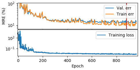
Figure A1Training errors, validation errors and training losses shown on a logarithmic scale. Although the training loss continues to slowly drop after the epoch with the lowest validation error (red line, at epoch 881), validation error stays relatively flat, suggesting that the ConvNet is overfitting after this epoch. The gradual decrease in MRE is less smooth than the training loss because the loss function is mean squared error, whereas the MRE is proportional to the mean absolute error.
MJM and TM conceived of the research idea, and MJM, TM and BW collected field data. The paper was written by MJM and edited by TM. HS wrote the code for processing the AUV data, and MJM wrote the code for analyzing the data.
The authors declare that they have no conflict of interest.
The authors would like to thank Jeff Anderson for overseeing the AUV surveys. Guy Williams and Alek Razdan were instrumental in collecting the AUV data. The crew on board the RV N.B. Palmer were also essential to the success of the PIPERS expedition. The references were compiled using JabRef.
This work was supported by the U.S. National Science Foundation (grant nos. ANT-1341606, ANT-1142075 and ANT-1341717) and NASA (grant no. NNX15AC69G).
This paper was edited by John Yackel and reviewed by Stefan Kern and two anonymous referees.
Akaike, H.: A new look at the statistical model identification, in: Selected Papers of Hirotugu Akaike, Springer, 215–222, https://doi.org/10.1007/978-1-4612-1694-0_16, 1974. a, b
Baldi, P.: Autoencoders, unsupervised learning, and deep architectures, in: Proceedings of ICML workshop on unsupervised and transfer learning, 37–49, 2012. a
Behrendt, A., Dierking, W., Fahrbach, E., and Witte, H.: Sea ice draft in the Weddell Sea, measured by upward looking sonars, Earth Syst. Sci. Data, 5, 209–226, https://doi.org/10.5194/essd-5-209-2013, 2013. a
Brock, J. C., Wright, C. W., Clayton, T. D., and Nayegandhi, A.: LIDAR optical rugosity of coral reefs in Biscayne National Park, Florida, Coral Reefs, 23, 48–59, https://doi.org/10.1007/s00338-003-0365-7, 2004. a
Dierking, W.: Laser profiling of the ice surface topography during the Winter Weddell Gyre Study 1992, J. Geophys. Res.-Oceans, 100, 4807–4820, https://doi.org/10.1029/94jc01938, 1995. a
Eicken, H. and Salganek, M.: Field techniques for Sea-ice Research, University of Alaska Press, 2010. a
Fons, S. W. and Kurtz, N. T.: Retrieval of snow freeboard of Antarctic sea ice using waveform fitting of CryoSat-2 returns, The Cryosphere, 13, 861–878, https://doi.org/10.5194/tc-13-861-2019, 2019. a
Goebell, S.: Comparison of coincident snow-freeboard and sea ice thickness profiles derived from helicopter-borne laser altimetry and electromagnetic induction sounding, J. Geophys. Res.-Oceans, 116, C08018, https://doi.org/10.1029/2009jc006055, 2011. a, b
Haas, C.: Evaluation of ship-based electromagnetic-inductive thickness measurements of summer sea-ice in the Bellingshausen and Amundsen Seas, Antarctica, Cold Reg. Sci. Technol., 27, 1–16, https://doi.org/10.1016/s0165-232x(97)00019-0, 1998. a
Haas, C., Liu, Q., and Martin, T.: Retrieval of Antarctic sea-ice pressure ridge frequencies from ERS SAR imagery by means of in situ laser profiling and usage of a neural network, Int. J. Remote Sens., 20, 3111–3123, https://doi.org/10.1080/014311699211642, 1999. a
Haas, C., Lobach, J., Hendricks, S., Rabenstein, L., and Pfaffling, A.: Helicopter-borne measurements of sea ice thickness, using a small and lightweight, digital EM system, J. Appl. Geophys., 67, 234–241, https://doi.org/10.1016/j.jappgeo.2008.05.005, 2009. a
Harms, S., Fahrbach, E., and Strass, V. H.: Sea ice transports in the Weddell Sea, J. Geophys. Res.-Oceans, 106, 9057–9073, https://doi.org/10.1029/1999jc000027, 2001. a
Haumann, F. A., Gruber, N., Münnich, M., Frenger, I., and Kern, S.: Sea-ice transport driving Southern Ocean salinity and its recent trends, Nature, 537, 7618, https://doi.org/10.1038/nature19101, 2016. a
Holland, M. M., Bitz, C. M., Hunke, E. C., Lipscomb, W. H., and Schramm, J. L.: Influence of the sea ice thickness distribution on polar climate in CCSM3, J. Climate, 19, 2398–2414, https://doi.org/10.1175/jcli3751.1, 2006. a
Holland, P. R., Bruneau, N., Enright, C., Losch, M., Kurtz, N. T., and Kwok, R.: Modeled trends in Antarctic sea ice thickness, J. Climate, 27, 3784–3801, https://doi.org/10.1175/jcli-d-13-00301.1, 2014. a
Hutchings, J. K., Heil, P., Lecomte, O., Stevens, R., Steer, A., and Lieser, J. L.: Comparing methods of measuring sea-ice density in the East Antarctic, Ann. Glaciol., 56, 77–82, https://doi.org/10.3189/2015aog69a814, 2015. a, b
Jeffrey Mei, M. et al.: Sea Ice Layer Cakes, PIPERS 2017, U.S. Antarctic Program (USAP) Data Center, https://doi.org/10.15784/601207, 2019. a
Kaleschke, L., Girard-Ardhuin, F., Spreen, G., Beitsch, A., and Kern, S.: ASI Algorithm SSMI-SSMIS sea ice concentration data, originally computed at and provided by IFREMER, Brest, France, were obtained as 5-day median-filtered and gap-filled product for 2017/06/02 from the Integrated Climate Date Center ICDC, available at: http://icdc.cen.uni-hamburg.de/1.html (last access: 20 August 2018), 2017. a
Kern, S. and Spreen, G.: Uncertainties in Antarctic sea-ice thickness retrieval from ICESat, Ann. Glaciol., 56, 107–119, https://doi.org/10.3189/2015aog69a736, 2015. a, b, c, d
Kern, S., Ozsoy-Çiçek, B., and Worby, A.: Antarctic sea-ice thickness retrieval from ICESat: Inter-comparison of different approaches, Remote Sens., 8, 538 pp., https://doi.org/10.3390/rs8070538, 2016. a, b
Kingma, D. P. and Ba, J.: Adam: A method for stochastic optimization, arXiv:1412.6980, https://arxiv.org/abs/1412.6980 (last access: 24 February 2019), 2014. a
Klambauer, G., Unterthiner, T., Mayr, A., and Hochreiter, S.: Self-normalizing neural networks, in: Advances in neural information processing systems, 971–980, available at: http://papers.nips.cc/paper/6698-self-normalizing-neural-networks (last access: 24 February 2019), 2017. a, b
Krizhevsky, A., Sutskever, I., and Hinton, G. E.: Imagenet classification with deep convolutional neural networks, in: Advances in neural information processing systems, 1097–1105, 2012. a
Kurtz, N.: IceBridge quick look sea ice freeboard, snow depth, and thickness product manual for 2013, Boulder, Colorado USA, NASA DAAC at the National Snow and Ice Data Center, 2013. a, b
Kurtz, N. and Markus, T.: Satellite observations of Antarctic sea ice thickness and volume, J. Geophys. Res.-Oceans, 117, C08025, https://doi.org/10.1029/2012jc008141, 2012. a, b
Onana, V., Kurtz, N. T., Farrell, S. L., Koenig, L. S., Studinger, M., and Harbeck, J. P.: A sea-ice lead detection algorithm for use with high-resolution airborne visible imagery, IEEE T. Geosci. Remote, 51, 38–56, https://doi.org/10.1109/tgrs.2012.2202666, 2012. a
Kwok, R. and Cunningham, G.: Variability of Arctic sea ice thickness and volume from CryoSat-2, Philos. T. Roy. Soc. A, 373, 20140157, https://doi.org/10.1098/rsta.2014.0157, 2015. a
Kwok, R. and Maksym, T.: Snow depth of the Weddell and Bellingshausen sea ice covers from IceBridge surveys in 2010 and 2011: An examination, J. Geophys. Res.-Oceans, 119, 4141–4167, https://doi.org/10.1002/2014jc009943, 2014. a, b, c
Kwok, R. and Rothrock, D.: Decline in Arctic sea ice thickness from submarine and ICESat records: 1958–2008, Geophys. Res. Lett., 36, L15501, https://doi.org/10.1029/2009gl039035, 2009. a
LeNail, A.: NN-SVG: Publication-Ready Neural Network Architecture Schematics, Journal of Open Source Software, 4, 747, https://doi.org/10.21105/joss.00747, 2019. a
Levi, G. and Hassner, T.: Age and gender classification using convolutional neural networks, in: Proceedings of the IEEE conference on computer vision and pattern recognition workshops, 34–42, 2015. a
Li, H., Xie, H., Kern, S., Wan, W., Ozsoy, B., Ackley, S., and Hong, Y.: Spatio-temporal variability of Antarctic sea-ice thickness and volume obtained from ICESat data using an innovative algorithm, Remote Sens. Environ., 219, 44–61, https://doi.org/10.1016/j.rse.2018.09.031, 2018. a, b
Li, S. and Chan, A. B.: 3d human pose estimation from monocular images with deep convolutional neural network, in: Asian Conference on Computer Vision, Springer, 332–347, 2014. a
Maksym, T., Leonard, K., Mei, M. J., Singh, H., Steer, A., Trujillo, E., Wever, N., Wilkinson, J., Williams, G., and White, S.: Snow depth distribution on Antarctic sea ice and its relationship with ice thickness, The Cryosphere, in preparation, 2019. a
Maksym, T. and Markus, T.: Antarctic sea ice thickness and snow-to-ice conversion from atmospheric reanalysis and passive microwave snow depth, J. Geophys. Res.-Oceans, 113, C02S12, https://doi.org/10.1029/2006jc004085, 2008. a
Markus, T. and Cavalieri, D. J.: Snow depth distribution over sea ice in the Southern Ocean from satellite passive microwave data, Antarctic sea ice: physical processes, interactions and variability, 19–39, https://doi.org/10.1029/ar074p0019, 1998. a, b
Markus, T., Massom, R., Worby, A., Lytle, V., Kurtz, N., and Maksym, T.: Freeboard, snow depth and sea-ice roughness in East Antarctica from in situ and multiple satellite data, Ann. Glaciol., 52, 242–248, https://doi.org/10.3189/172756411795931570, 2011. a
Markus, T., Neumann, T., Martino, A., Abdalati, W., Brunt, K., Csatho, B., Farrell, S., Fricker, H., Gardner, A., Hardin, D., Jasinski, M., Kwok, R., Magruder, L., Lubin, D., Luthcke, S., Morison, J., Nelson, R., Neuenschwander, A., Palm, S., Popescu, S., Shum, C. K., Schutz, B. E., Smith, B., Yang, Y., and Zwally, J.: The Ice, Cloud, and land Elevation Satellite-2 (ICESat-2): science requirements, concept, and implementation, Remote Sens. Environ., 190, 260–273, https://doi.org/10.1016/j.rse.2016.12.029, 2017. a
Massonnet, F., Mathiot, P., Fichefet, T., Goosse, H., Beatty, C. K., Vancoppenolle, M., and Lavergne, T.: A model reconstruction of the Antarctic sea ice thickness and volume changes over 1980–2008 using data assimilation, Ocean Model., 64, 67–75, https://doi.org/10.1016/j.ocemod.2013.01.003, 2013. a, b
Ozsoy-Cicek, B., Kern, S., Ackley, S. F., Xie, H., and Tekeli, A. E.: Intercomparisons of Antarctic sea ice types from visual ship, RADARSAT-1 SAR, Envisat ASAR, QuikSCAT, and AMSR-E satellite observations in the Bellingshausen Sea, Deep-Sea Res. Pt. II, 58, 1092–1111, https://doi.org/10.1016/j.dsr2.2010.10.031, 2011. a
Ozsoy-Cicek, B., Ackley, S., Xie, H., Yi, D., and Zwally, J.: Sea ice thickness retrieval algorithms based on in situ surface elevation and thickness values for application to altimetry, J. Geophys. Res.-Oceans, 118, 3807–3822, https://doi.org/10.1002/jgrc.20252, 2013. a, b, c, d, e, f, g, h, i, j, k, l, m, n, o, p, q, r
Parkinson, C. L. and Cavalieri, D. J.: Antarctic sea ice variability and trends, 1979–2010, The Cryosphere, 6, 871–880, https://doi.org/10.5194/tc-6-871-2012, 2012. a
Rothrock, D., Percival, D., and Wensnahan, M.: The decline in Arctic sea-ice thickness: Separating the spatial, annual, and interannual variability in a quarter century of submarine data, J. Geophys. Res.-Oceans, 113, C05003, https://doi.org/10.1029/2007jc004252, 2008. a
Shalev-Shwartz, S. and Ben-David, S.: Understanding machine learning: From theory to algorithms, Cambridge University Press, https://doi.org/10.1017/cbo9781107298019, 2014. a
Shu, Q., Song, Z., and Qiao, F.: Assessment of sea ice simulations in the CMIP5 models, The Cryosphere, 9, 399–409, https://doi.org/10.5194/tc-9-399-2015, 2015. a
Sibson, R.: A Brief Description of Natural Neighbor Interpolation, in: Interpreting Multivariate Data, edited by: Barnett, V., John Wiley & Sons, New York, 21–36, 1981. a, b
Srivastava, N., Hinton, G., Krizhevsky, A., Sutskever, I., and Salakhutdinov, R.: Dropout: a simple way to prevent neural networks from overfitting, J. Mach. Learn. Res., 15, 1929–1958, 2014. a, b
Stammerjohn, S.: NBP1704 CTD sensor data, U.S. Antarctic Program (USAP) Data Center, https://doi.org/10.15784/601192, 2019. a
Stammerjohn, S., Martinson, D., Smith, R., Yuan, X., and Rind, D.: Trends in Antarctic annual sea ice retreat and advance and their relation to El Niño–Southern Oscillation and Southern Annular Mode variability, J. Geophys. Res.-Oceans, 113, C03S90, https://doi.org/10.1029/2007jc004269, 2008. a
Stroeve, J. C., Markus, T., Maslanik, J. A., Cavalieri, D. J., Gasiewski, A. J., Heinrichs, J. F., Holmgren, J., Perovich, D. K., and Sturm, M.: Impact of surface roughness on AMSR-E sea ice products, IEEE T. Geosci. Remote, 44, 3103–3117, https://doi.org/10.1109/TGRS.2006.880619, 2006. a
Strub-Klein, L. and Sudom, D.: A comprehensive analysis of the morphology of first-year sea ice ridges, Cold Reg. Sci. Technol., 82, 94–109, https://doi.org/10.1016/j.coldregions.2012.05.014, 2012. a
Sturm, M. and Holmgren, J.: An Automatic Snow Depth Probe for Field Validation Campaigns, Water Resour. Res., 54, 9695–9701, https://doi.org/10.1029/2018wr023559, 2018. a
Sturm, M., Morris, K., and Massom, R.: The winter snow cover of the West Antarctic pack ice: its spatial and temporal variability, Antarctic sea ice: physical processes, interactions and variability, 1–18, https://doi.org/10.1029/ar074p0001, 1998. a, b
Timco, G. and Burden, R.: An analysis of the shapes of sea ice ridges, Cold Reg. Sci. Technol., 25, 65–77, https://doi.org/10.1016/s0165-232x(96)00017-1, 1997. a
Timco, G. and Frederking, R.: A review of sea ice density, Cold Reg. Sci. Technol., 24, 1–6, https://doi.org/10.1016/0165-232x(95)00007-x, 1996. a
Timco, G. and Weeks, W.: A review of the engineering properties of sea ice, Cold Reg. Sci. Technol., 60, 107–129, https://doi.org/10.1016/j.coldregions.2009.10.003, 2010. a
Tin, T. and Jeffries, M. O.: Sea-ice thickness and roughness in the Ross Sea, Antarctica, Ann. Glaciol., 33, 187–193, https://doi.org/10.3189/172756401781818770, 2001. a
Tin, T. and Jeffries, M. O.: Morphology of deformed first-year sea ice features in the Southern Ocean, Cold Reg. Sci. Technol., 36, 141–163, https://doi.org/10.1016/s0165-232x(03)00008-9, 2003. a, b, c, d, e, f
Turner, J., Bracegirdle, T. J., Phillips, T., Marshall, G. J., and Hosking, J. S.: An initial assessment of Antarctic sea ice extent in the CMIP5 models, J. Climate, 26, 1473–1484, https://doi.org/10.1175/jcli-d-12-00068.1, 2013. a
Urabe, N. and Inoue, M.: Mechanical properties of Antarctic sea ice, J. Offshore Mech. Arct., 110, 403–408, https://doi.org/10.1115/1.3257079, 1988. a
van der Maaten, L. and Hinton, G.: Visualizing data using t-SNE, J. Mach. Learn. Res., 9, 2579–2605, 2008. a, b
Weissling, B. and Ackley, S.: Antarctic sea-ice altimetry: scale and resolution effects on derived ice thickness distribution, Ann. Glaciol., 52, 225–232, https://doi.org/10.3189/172756411795931679, 2011. a
Willatt, R. C., Giles, K. A., Laxon, S. W., Stone-Drake, L., and Worby, A. P.: Field investigations of Ku-band radar penetration into snow cover on Antarctic sea ice, IEEE T. Geosci. Remote, 48, 365–372, https://doi.org/10.1109/tgrs.2009.2028237, 2009. a
Williams, G., Maksym, T., Wilkinson, J., Kunz, C., Murphy, C., Kimball, P., and Singh, H.: Thick and deformed Antarctic sea ice mapped with autonomous underwater vehicles, Nat. Geosci., 8, 61–67, https://doi.org/10.1038/ngeo2299, 2015. a, b, c, d, e, f, g
Williams, G. D., Maksym, T., Kunz, C., Kimball, P., Singh, H., Wilkinson, J., Lachlan-Cope, T., Trujillo, E., Steer, A., Massom, R., Meiners, K., Heil, P., Lieser, J., Leonard, K., and Murphy, C.: Beyond point measurements: Sea ice floes characterized in 3-D, EOS T. Am. Geophys. Un., 94, 69–70, https://doi.org/10.1002/2013eo070002, 2013. a
Wingham, D. J., Francis, C. R., Baker, S., Bouzinac, C., Brockley, D., Cullen, R., de Chateau-Thierry, P., Laxon, S. W., Mallow, U., Mavrocordatos, C., Phalippou, L., Ratier, G., Rey, L., Rostan, F., Viau, P., and Wallis, D. W.: CryoSat: A mission to determine the fluctuations in Earth's land and marine ice fields, Adv. Space Res., 37, 841–871, https://doi.org/10.1016/j.asr.2005.07.027, 2006. a
Worby, A., Jeffries, M., Weeks, W., Morris, K., and Jana, R.: The thickness distribution of sea ice and snow cover during late winter in the Bellingshausen and Amundsen Seas, Antarctica, J. Geophys. Res.-Oceans, 101, 28441–28455, https://doi.org/10.1029/96jc02737, 1996. a
Worby, A., Bush, G., and Allison, I.: Seasonal development of the sea-ice thickness distribution in East Antarctica: Measurements from upward-looking sonar, Ann. Glaciol., 33, 177–180, https://doi.org/10.3189/172756401781818167, 2001. a
Worby, A. P., Geiger, C. A., Paget, M. J., Van Woert, M. L., Ackley, S. F., and DeLiberty, T. L.: Thickness distribution of Antarctic sea ice, J. Geophys. Res.-Oceans, 113, C05S92, https://doi.org/10.1029/2007jc004254, 2008. a, b, c, d, e
Worby, A. P., Steer, A., Lieser, J. L., Heil, P., Yi, D., Markus, T., Allison, I., Massom, R. A., Galin, N., and Zwally, J.: Regional-scale sea-ice and snow thickness distributions from in situ and satellite measurements over East Antarctica during SIPEX 2007, Deep-Sea Res. Pt. II, 58, 1125–1136, https://doi.org/10.1016/j.dsr2.2010.12.001, 2011. a
Xie, H., Ackley, S., Yi, D., Zwally, H., Wagner, P., Weissling, B., Lewis, M., and Ye, K.: Sea-ice thickness distribution of the Bellingshausen Sea from surface measurements and ICESat altimetry, Deep-Sea Res. Pt. II, 58, 1039–1051, https://doi.org/10.1016/j.dsr2.2010.10.038, 2011. a, b, c
Xie, H., Tekeli, A. E., Ackley, S. F., Yi, D., and Zwally, H. J.: Sea ice thickness estimations from ICESat Altimetry over the Bellingshausen and Amundsen Seas, 2003–2009, J. Geophys. Res.-Oceans, 118, 2438–2453, https://doi.org/10.1002/jgrc.20179, 2013. a, b, c
Yi, D., Zwally, H. J., and Robbins, J. W.: ICESat observations of seasonal and interannual variations of sea-ice freeboard and estimated thickness in the Weddell Sea, Antarctica (2003–2009), Ann. Glaciol., 52, 43–51, https://doi.org/10.3189/172756411795931480, 2011. a
Yi, D., Harbeck, J. P., Manizade, S. S., Kurtz, N. T., Studinger, M., and Hofton, M.: Arctic sea ice freeboard retrieval with waveform characteristics for NASA's Airborne Topographic Mapper (ATM) and Land, Vegetation, and Ice Sensor (LVIS), IEEE T. Geosci. Remote, 53, 1403–1410, https://doi.org/10.1109/tgrs.2014.2339737, 2015. a
Zeiler, M. D. and Fergus, R.: Visualizing and understanding convolutional networks, in: European conference on computer vision, Springer, 818–833, https://doi.org/10.1007/978-3-319-10590-1_53, 2014. a
Zwally, H. J., Yi, D., Kwok, R., and Zhao, Y.: ICESat measurements of sea ice freeboard and estimates of sea ice thickness in the Weddell Sea, J. Geophys. Res.-Oceans, 113, C02S15, https://doi.org/10.1029/2007jc004284, 2008. a, b, c, d, e, f