the Creative Commons Attribution 4.0 License.
the Creative Commons Attribution 4.0 License.
 | 26 Nov 2019
Subglacial roughness of the Greenland Ice Sheet: relationship with contemporary ice velocity and geology
Michael A. Cooper
Thomas M. Jordan
Dustin M. Schroeder
Martin J. Siegert
Christopher N. Williams
Jonathan L. Bamber
The subglacial environment of the Greenland Ice Sheet (GrIS) is poorly constrained both in its bulk properties, for example geology, the presence of sediment, and the presence of water, and interfacial conditions, such as roughness and bed rheology. There is, therefore, limited understanding of how spatially heterogeneous subglacial properties relate to ice-sheet motion. Here, via analysis of 2 decades of radio-echo sounding data, we present a new systematic analysis of subglacial roughness beneath the GrIS. We use two independent methods to quantify subglacial roughness: first, the variability in along-track topography – enabling an assessment of roughness anisotropy from pairs of orthogonal transects aligned perpendicular and parallel to ice flow and, second, from bed-echo scattering – enabling assessment of fine-scale bed characteristics. We establish the spatial distribution of subglacial roughness and quantify its relationship with ice flow speed and direction. Overall, the beds of fast-flowing regions are observed to be rougher than the slow-flowing interior. Topographic roughness exhibits an exponential scaling relationship with ice surface velocity parallel, but not perpendicular, to flow direction in fast-flowing regions, and the degree of anisotropy is correlated with ice surface speed. In many slow-flowing regions both roughness methods indicate spatially coherent regions of smooth beds, which, through combination with analyses of underlying geology, we conclude is likely due to the presence of a hard flat bed. Consequently, the study provides scope for a spatially variable hard- or soft-bed boundary constraint for ice-sheet models.


The rate of global sea-level rise contributions from the Greenland Ice Sheet (GrIS) has accelerated over the past 2 decades (Velicogna and Wahr, 2006; Rignot et al., 2011; Mottram et al., 2019); increasing rates of mass loss, driving this acceleration, are partitioned between ice discharge (over the grounding line) and, more recently, enhanced surface melt (Enderlin et al., 2014; van den Broeke et al., 2016, 2017; Hofer et al., 2017; McMillan et al., 2016; Fettweis et al., 2017; Mouginot et al., 2019; Mottram et al., 2019). To constrain projections for future change, models must parameterise characteristics influencing ice-sheet motion and dynamics (e.g. Huybrechts, 1994; Nick et al., 2013). Outlet regions, and in particular fast-flowing ice streams, are principally characterised by enhanced basal motion (basal sliding; Cuffey and Paterson, 2010; van der Veen, 2013). Conditions attributed to, and rates of, sliding at the bed are influenced by various properties of the subglacial environment, including, but not limited to, basal thermal regime, presence of basal water (and effective pressure), rheological bed properties (i.e. the presence of sediment and its viscosity or deformability), and basal friction (or traction; i.e. resistance from bed roughness; Weertman, 1957; Nye, 1970; Durand et al., 2011; Clarke, 2004; Iverson and Zoet, 2015; Brondex et al., 2017; Stearns and van der Veen, 2018). Although the influence of these processes on ice flow and dynamics is generally well understood (at least theoretically using idealised models; Cuffey and Paterson, 2010; van der Veen, 2013), it is not incorporated into ice-sheet models as spatially varying boundary conditions. Understanding the spatial variation in subglacial conditions and processes remains restricted by the paucity of observations; as such, necessary model parameters are often inverted or inferred.
Fundamentally, ice-sheet models rely on the application of sliding laws to approximate the rate of basal motion with regards to subglacial characteristics. Whilst several sliding laws exist, each variously influencing the behaviour and sensitivity of modelled glacier response (Brondex et al., 2017), most models rely on a Weertman-style hard-bed sliding law (Weertman, 1957, 1972; Stearns and van der Veen, 2018). In this case, sliding velocity, and thus broad characteristics of ice dynamics, are controlled by frictional stresses induced at the ice–bed interface as a result of small-scale “obstacles” (with a wavelength, or length scale, on the order of ∼1 m) superimposed onto subglacial topography (with a length scale on the order of ∼100–1000 m Weertman, 1957; Nye, 1970; Iverson and Zoet, 2015; Stearns and van der Veen, 2018). Such fine-scale obstacles are not resolved within widely available gridded bed topography products (e.g. Bedmap2 and BedMachine V3 in Fretwell et al., 2013, and Morlighem et al., 2017, respectively), and direct observation is not possible through conventional (i.e. topographic) subglacial-roughness quantification methods utilising radio-echo sounding (RES) data (as described below). Furthermore, the scale at which friction is induced by these features is much less than can be resolved within numerical ice-sheet modelling. As such, “basal traction” is primarily simulated (inferred) using satellite-derived surface velocity (e.g. Joughin et al., 2009; Gillet-Chaulet et al., 2012; Arthern et al., 2015), with basal sliding inverted by optimally matching the model velocity to observations through the reduction of basal traction beneath specific regions of enhanced ice flow.
The quantification of subglacial roughness, and subsequent evaluation with regard to ice velocity, has been the focus of many studies in recent years across Antarctica (e.g. Siegert et al., 2005; Rippin et al., 2006, 2014; Bingham and Siegert, 2007, 2009; Schroeder et al., 2014) and Greenland, though to a lesser extent (e.g. Layberry and Bamber, 2001; Rippin, 2013; Lindbäck and Pettersson, 2015; Jordan et al., 2017). Whilst subglacial roughness appears to exert control on the location of fast-flowing streaming ice (Siegert et al., 2004; Rippin et al., 2006, 2014; Bingham and Siegert, 2007, 2009), its influence or behaviour with respect to ice motion is not universal. Existing roughness maps of Greenland (i.e. Rippin, 2013; Jordan et al., 2017) show that fast flow can be associated with rougher beds, where slow-flowing regions are more smooth. As the majority of studies to date quantify large-scale topographic-roughness information (on the order of ∼1000 m), any direct influence on basal traction, if at all, remains unclear. However, a recent high-resolution assessment (sub-kilometre) of bed topography beneath the Pine Island Glacier has concluded that small-scale bed features (on the order of ∼10–100 m) do indeed influence ice motion, principally through the induction of basal drag controlled by the orientation and size of subglacial obstacles (Bingham et al., 2017).
Assessing subglacial-roughness information with respect to ice motion, however, is not limited to basal traction, particularly when defined at varying length scales. When considering roughness signatures, Bingham and Siegert (2009) present a clear conceptual framework for examining the causes and controls of smooth and rough beds in both hard- and soft-bed scenarios. For example, the majority of roughness studies of the West Antarctic Ice Sheet bed have associated low roughness (i.e. smooth beds) with the presence of deformable sediment (e.g. Rippin et al., 2006, 2011, 2014; Bingham and Siegert, 2007, 2009; Schroeder et al., 2014); however, it is evident that streamlined bedrock (hard beds) can also promote smooth-bed signals (e.g. Siegert et al., 2005; Rippin et al., 2014; Jeofry et al., 2018). The link between the presence of saturated (wet), deformable sediments, and ice motion was first identified on the Siple Coast, West Antarctica, by Blankenship et al. (1986) and Alley et al. (1986), where it is seen to control both the onset and magnitude of fast flow (Peters et al., 2006; Siegert et al., 2016). Whilst flow configuration of the Greenland Ice Sheet is markedly different (with regard to streaming ice), recent regional studies have documented the presence of soft basal sediments underlying fast-flowing outlet glaciers (Christianson et al., 2014; Kulessa et al., 2017; Hofstede et al., 2018), where it is, potentially, seen as an important control on ice flow in Greenland (Bougamont et al., 2014). Furthermore, recent characterisation of the majority of Greenland's outlet glaciers implies that the role of effective basal water pressure (as well as the availability of deformable sediment) is more important and influential than basal friction itself (Stearns and van der Veen, 2018); however, it should be noted that this conclusion, and the role of friction in basal slip, is contested (Minchew et al., 2019). Altogether, this suggests not only that a consideration of orientation (or anisotropy) in the interpretation of subglacial roughness is necessary but also that basal motion relies on the influence of other factors (e.g. basal thermal state, geographic or geological setting, and/or the presence of sediment; Bingham and Siegert, 2009).
Limited direct information regarding the geology of Greenland is available; however, well-constrained boundaries at the ice-free margins are extrapolated inland, facilitated by a geophysical survey (i.e. measuring gravity or magnetic anomalies; Henriksen, 2008; Dawes, 2009). Much of the island is underlain by stable crystalline rocks of the Precambrian, where younger mountain chains, formed by the Caledonian (∼420 Ma ago) and the Ellesmerian fold belts (∼350 Ma ago), run parallel to the coast in north-eastern and northern Greenland, respectively (Henriksen, 2008; Dawes, 2009). Localised volcanic intrusions are documented at the margins of southern and south-eastern Greenland (Dawes, 2009), with smaller intrusions documented subglacially by Tinto et al. (2015) in the locality of Petermann Glacier (PG; see Fig. 1).
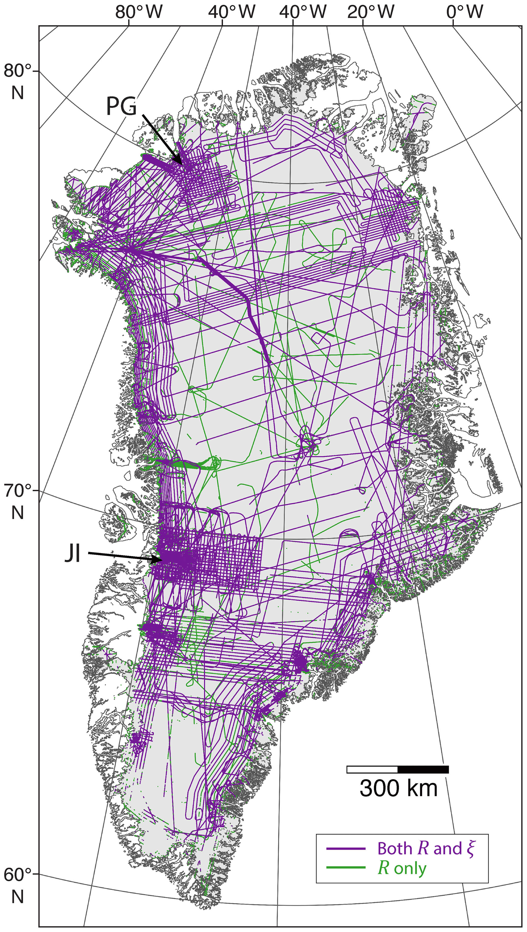
Figure 1Coverage of radar sounding surveys over the GrIS used in this study. Topography-derived (topographic) roughness (R) is calculated using all available CReSIS survey data between 1993 and 2016, where scattering-derived roughness (ξ) uses only a subset of these (further explained in Sect. 2.3). JI and PG highlight the dense-grid sampling regime used over the Jakobshavn Isbræand Petermann Glacier catchments (as referred to in Sect. 3.1), displayed using a polar stereographic north projection (71∘ N, 39∘ W), as with all other spatial plots.
Conclusions drawn from previous quantifications of subglacial roughness in Greenland are limited. Whilst the broad, ice-sheet-wide distribution of roughness has been mapped (Layberry and Bamber, 2001; Rippin, 2013), systematic comparison to ice motion, and in particular the relationship between roughness anisotropy and flow direction, has not been fully considered. Rippin (2013) presents the most recent ice-sheet-wide depiction of subglacial roughness in Greenland. Whilst this highlighted the spatial distribution of roughness information across the island, a non-uniform conclusion was made with regard to ice surface speed (ice surface velocity magnitude, ). Furthermore, the method employed aggregated information across various length scales, working to eliminate more-fine-scale information. More recently, Lindbäck and Pettersson (2015) present a study (albeit spatially limited) highlighting the importance of considering roughness anisotropy, referencing ice motion. The recent increase in coverage of RES data over the GrIS (Rodriguez-Morales et al., 2014; Morlighem et al., 2017), so far unused in roughness analysis, provides a new opportunity to increase understanding of the subglacial environment, enabling an ice-sheet-wide description of spatially heterogeneous bulk (i.e. geology and the presence of sediment) and interfacial properties (i.e. roughness and rheological bed properties).
Subglacial-roughness information can be obtained from RES data in two ways: firstly, via the statistical properties of along-track topography (e.g. Hubbard et al., 2000; Taylor et al., 2004; Siegert et al., 2005; Rippin, 2013; Goff et al., 2014) and, secondly, via the electromagnetic scattering properties of the bed-echo waveform (e.g. Oswald and Gogineni, 2008; Schroeder et al., 2013; Young et al., 2016; Jordan et al., 2017). Topography-derived roughness can be obtained using both the space domain (e.g. measuring the root-mean-square – RMS – height as a function of horizontal length scale) and the frequency domain or spectral methods (e.g. performing a Fourier transform; Shepard et al., 1995; Hubbard et al., 2000; Shepard et al., 2001; Smith, 2014). The length scale over which topographic roughness is assessed is limited to being greater than the horizontal resolution of the RES measurements (typically 30 m or greater; Taylor et al., 2004; Li et al., 2010; Jordan et al., 2017). Scattering-derived roughness is sensitive to the radio wavelength in ice (typically 1–5 m for most radar systems) and reveals more-fine-scale geometric information about the subglacial interface than topographic analysis (Shepard et al., 2001; Berry, 1973; Schroeder et al., 2015; Jordan et al., 2017).
One simple approach to mapping subglacial information from electromagnetic scattering is to use the “abruptness” (or “pulse peakiness”) of the bed-echo waveform (Oswald and Gogineni, 2008, 2012; Young et al., 2016; Jordan et al., 2017). This parameter, defined as the ratio of peak to integrated bed-echo power, gives an indication of the relative contributions of specular reflection (presenting higher abruptness, associated with fine-scale smooth beds) and diffuse scattering and clutter (presenting lower abruptness, associated with fine-scale rough beds). RES flight-track maps for the bed-echo abruptness in northern and central Greenland demonstrate clear spatial structure (Oswald and Gogineni, 2008, 2012; Jordan et al., 2017). For example, there are near-continuous regions of high abruptness in the interior (e.g. near the Camp Century and NorthGRIP ice cores; Oswald and Gogineni, 2008, 2012; Jordan et al., 2017), whereas many ice margin regions have lower abruptness levels (e.g. the main trunk of Petermann Glacier; Jordan et al., 2017). The original geophysical interpretation of the larger-scale high-abruptness regions (typically 100s of square kilometres) is that they often represent extended, electrically deep (>8 m; Gorman and Siegert, 1999) bodies of basal water (Oswald and Gogineni, 2008, 2012). However, this picture is largely inconsistent with ice core temperature data and existing knowledge of the basal thermal state (MacGregor et al., 2016; Jordan et al., 2017). An alternative explanation is that the larger-scale high-abruptness regions typically indicate smooth bedrock, with deep water only likely being present in localised patches (Jordan et al., 2017). This primarily lithological interpretation of the bed-echo abruptness has, however, yet to be fully explored and integrated with existing knowledge of ice dynamics and subglacial geology.
In this paper, using 2 decades of Center for Remote Sensing of Ice Sheets (CReSIS) RES data, we present a new systematic analysis for subglacial roughness beneath the Greenland Ice Sheet (GrIS). We outline two independent methods for quantifying roughness using information obtained via both statistical analysis of sampled bed elevation (hereafter termed topographic roughness; Sect. 2.2) and the scattering properties quantified from the bed-echo waveform (hereafter termed scattering-derived roughness; Sect. 2.3). We map the spatial distribution of subglacial roughness across the GrIS (Sect. 3) and document a marked spatial heterogeneity using both metrics. We then assess roughness anisotropy (Sect. 3.2), providing clear evidence for direction dependence (anisotropy) between topographic roughness and the surface speed of ice in fast-flowing regions, both at the ice-sheet-scale and locally, surrounding major outlet glaciers. Finally, to better understand the observed coherent signal of “smooth” beds in regions of slow ice flow, we compare scattering-derived roughness to predicted underlying geology (Sect. 4.3).
2.1 Ice-penetrating radar systems and survey coverage
The RES data used in this study were collected by the CReSIS over the years 1993–2016, with more-recent campaigns undertaken as part of the wider Operation IceBridge (OIB) programme (post-2009). Surveys were typically undertaken between the months of March and May, using three airborne platforms: a P-3B Orion (P3), a DHC-6 Twin Otter (TO), and a Douglas DC-8 (DC8; Paden, 2017). The instruments used were, successively, the Improved Coherent Radar Depth Sounder (ICORDS), ICORDS – version 2 (v2), Advanced Coherent Radar Depth Sounder (ACORDS), Multi-Channel Radar Depth Sounder (MCRDS), Multi-Channel Coherent Radar Depth Sounder (MCoRDS), and MCoRDs v2 (Paden, 2017). Centre frequencies for the radar instruments are 149 MHz (for ICORDS and ICORDS v2), 150 MHz (for ACORDS and MCRDS), and 195 MHz (for MCoRDs and MCoRDS v2). The vertical (depth-range) resolution varies from ∼4.3 to 20 m, where the horizontal (along-track) resolution is typically ∼30 to 60 m. A precise breakdown of the radar data coverage by field season and radar instrument class can be found in (Fig. 1; MacGregor et al., 2015) and (Fig. 1; Jordan et al., 2018), respectively.
For measures of topographic roughness (Sect. 2.2) data across all campaigns were used; however, for scattering-derived roughness analysis (Sect. 2.3), only a subset of these are incorporated (indicated in Fig. 1), including ACORDS, MCRDS and MCoRDS, and MCoRDs v2 data. The rationale for this, relating to internal consistency when combining data from different radar instruments, is described in Sect. 2.3. Additionally, owing to the preference for “repeat fly-bys” in airborne sampling regimes, and the marked increase in survey kilometres in recent years (Rodriguez-Morales et al., 2014; Morlighem et al., 2017), the final spatial coverage of both roughness metrics is similar (Fig. 1).
Method-specific data pre-processing (i.e. the handling of quality flags) is described below. For full information regarding the multiple radar instruments used in this analysis, readers are referred to the user's guide (available at http://data.cresis.ku.edu/data/rds/rds_readme.pdf, last access: November 2019; Paden, 2017). Additionally, detailed signal processing steps, and information regarding data segmentation, are described in several previous works (i.e. Gogineni et al., 2001, 2014; Rodriguez-Morales et al., 2014; MacGregor et al., 2015; Paden, 2017).
2.2 Subglacial roughness from along-track topography
2.2.1 Calculating RMS height, R
As noted, subglacial-roughness information can be determined via the statistical analysis of vertical variation in along-track bed topography (e.g. Siegert et al., 2004, 2005; Taylor et al., 2004; Rippin et al., 2006, 2011, 2014; Bingham and Siegert, 2007, 2009; Bingham et al., 2007, 2017; Li et al., 2010; Rippin, 2013). The most prevalent method in glaciological literature employs spectral methods to do this (i.e. the application of fast Fourier transforms – FFTs – first employed in glaciology by Hubbard et al., 2000, and for the Antarctic Ice Sheet by Taylor et al., 2004). Alternative space-domain methods exist, however, and are frequently used within earth and planetary sciences (Shepard et al., 2001; Smith, 2014).
Here, the first metric for subglacial roughness we present, topographic roughness (or R), is quantified by the RMS height in along-track topography (RES sampled bed elevation). The RMS height (referred to also as the standard deviation of bed elevation; e.g. Rippin et al., 2006, 2014) provides several benefits over the use of FFTs. First, it enables the collation of all CReSIS survey campaigns despite variable sample spacing (horizontal resolution) without requiring along-track interpolation or re-sampling of data. Second, this method allows the use of a shorter length scale than FFTs, not only facilitating subsequent anisotropic analysis at crossovers (Sect. 2.2.2) but also providing a finer-scale roughness information. A final advantage is that RMS height calculations are unit-preserving (i.e. quantifying variation at the bed in units of metres), providing a more physically intuitive metric. More critically, however, the spatial distribution of roughness values quantified by FFT and RMS height methods have been noted to be similar (Rippin et al., 2014; Falcini et al., 2018).
Sampled bed and surface elevations were obtained from all the available CReSIS RES surveys between 1993 and 2016. Where applicable, data were filtered using the provided quality flags denoting the confidence of the bed pick accuracy (Paden, 2017), ensuring that only bed elevations with “high” confidence were used; however, as RES data obtained during OIB campaigns prior to 2008, with the exception of the reprocessed “2006 TO” survey, do not include quality flags, all available sampled bed elevations were used. More-recent surveys (post-2006) have an increased along-track sampling resolution (approximately twice that of previous campaigns), owing to SAR processing and multi-looking stages in data preparation. This results in an “overlap” between consecutive samples of bed elevation (John Paden, personal communication, 2016). Therefore, to ensure that only independent measures of bed elevation are used for roughness calculation, data from these campaigns are rarefied (to include every other sample point).
Topographic roughness, R, is given by
where n is the number of sample points, z(xi) is the height of the surface point at point xi, and is the mean height of the profile over all xi values. RMS height R was calculated using a window length or bin size, L, of 200 m, using all recorded bed elevations, regardless of spatial density within the bin, provided that n≥3. R is given for the spatial midpoint of each window. Regions of greater roughness, quantified by a larger variation in bed elevation within the window, have greater R values. An example of R calculated along track using the sampled bed elevation is presented in Fig. 2. It should be noted that not all bins have a constant n due to the variation in sampling regime, the resolution of the different radar instruments, and data quality. R was not calculated for bins where n<3. Although n is small (mean is ∼8), we obtain a large sample size for calculating roughness statistics through the repeated sampling over multiple bins (using repeat flight tracks).
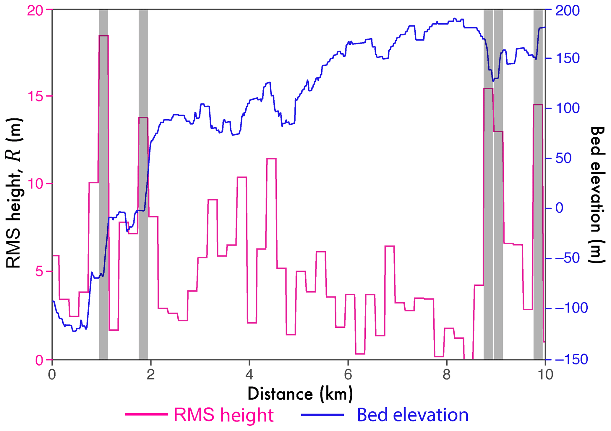
Figure 2Along-track example of calculated topographic roughness (R). This demonstrates the length scale (200 m) over which R is calculated from sampled bed elevation. Grey bars depict high values of R associated with subglacial step changes in elevation (“cliffs”); the limitation of interpreting topographic roughness in these regimes is discussed in Sect. 4.4.
L=200 m was chosen to enable the finest scale of R to be quantified whilst maintaining the largest spatial coverage of the resultant metric by using all available survey data. It is possible to quantify R at a finer scale using only more-recent survey data; however this is at the expense of reduced spatial coverage for a length scale not less than 100 m (limited by the along-track sample spacing). Changes in L influence the quantification of roughness as a result of the self-affine (fractal) scaling behaviour of subglacial terrain: as L increases, bed profiles with a steeper slope tend to become more rough relative to those with shallower slope (see Figs. 3, 1, and 2a, respectively, in Shepard et al., 1995, Shepard and Campbell, 1999, and Jordan et al., 2017).
2.2.2 Filtering R with respect to ice surface velocity
To evaluate, and more completely understand, how the spatial distribution of subglacial roughness influences or perhaps is influenced by ice-sheet motion, we compare R to ice surface velocities. We use the InSAR-derived MEaSUREs velocity mosaic (Joughin et al., 2016, 2017) over the entire GrIS. This mosaic helps with capturing long-term information (using 1995–2015 observations) regarding flow configuration, minimising inter- and intra-annual variation in both ice speed and direction. As R is quantified using 2 decades of RES data, we assume an inherent constancy in roughness over time. The MEaSUREs data provide magnitude (; speed) and direction at a 250 m resolution (Fig. 3a and b); however, for our analysis, we performed a bilinear aggregation (to 1000 m) in order to smooth small-scale variation or noise.
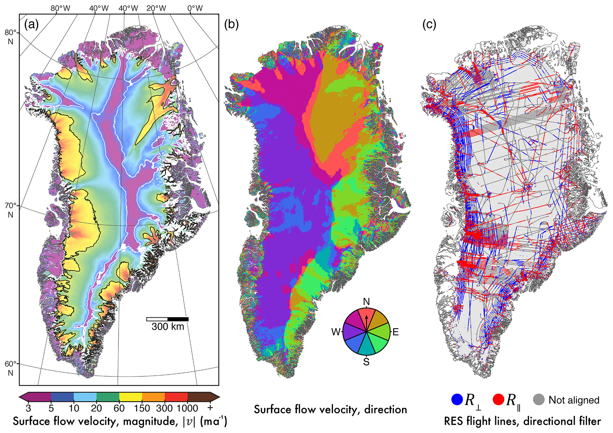
Figure 3Observed surface ice velocity characteristics of the GrIS used in the filtering of R. (a) InSAR-derived ice surface speed (velocity magnitude; m a−1; Joughin et al., 2016); regions of fast ( ma−1) and slow ( ma−1) flow are demarcated by the black and white contour lines, respectively. (b) Flow direction of ice surface from (a); coloured pinwheel denotes direction of surface ice flow, where north is at the top of the page. (c) Radar sounding surveys as in Fig. 1, filtered for alignment with surface flow direction (b); flight tracks are categorised as aligned either parallel (R∥) or perpendicular (R⟂) to surface flow direction (with a ±20∘ threshold) for the analysis of topographic-roughness anisotropy.
With regard to ice surface flow speed, we delineate regions of “fast” ( 50 ma−1) and “slow” ( ma−1) flow (Fig. 3a). In regions where exceeds 50 ma−1, ice is likely to be decoupled from the bed (i.e. sliding), as this speed cannot be achieved by internal deformation alone (MacGregor et al., 2016; Stearns and van der Veen, 2018). As we have noted above, basal traction, a principal constraint on basal sliding (Weertman, 1957), may be influenced by subglacial roughness (Siegert et al., 2004, 2005; Bingham et al., 2017). Second, where ice motion is limited in slow-flowing regions, rates of basal erosion are minimal and, thus, the influence on subglacial topography is reduced (Bingham and Siegert, 2009).
As R is quantified along track, there is an inherent directionality in its characterisation of the subglacial environment. To assess anisotropy at the bed, with particular reference to ice motion, we classify R through its alignment with local flow direction. Sample windows were filtered for their linearity to remove measures of R over corners and bends (with a deviation ≥10 %; after Bingham et al., 2015) in RES flight lines. Roughness bins were then filtered by their alignment to local surface ice flow direction (Fig. 3b) with a 20∘ threshold; Fig. 3c shows classified measures of R aligned perpendicularly R⟂ or in parallel R∥. From this, we draw conclusions based on the relationship between subglacial roughness and the speed of overlying ice. It should be noted that we only use contemporary ice velocity observations in this study; although flow configuration is likely to have remained largely constant, the surface speed will have changed through time. In terms of fractional error and uncertainty regarding ice speed and flow direction, and thus the classified alignment of roughness bins, slow-flowing regions represent the worst-case scenario. General error propagation formulae for independent velocity vectors (vx and vy) were applied, giving a mean error of 0.51 m a−1 for and 14.55∘ for direction, of which the latter is less than the larger angular threshold used to classify the alignment of roughness bins with respect to velocity.
Where coincident measures of R⟂ and R∥ are available (the near-orthogonal crossovers between flight lines), the degree of anisotropy can be calculated. This is achieved through a normalised difference ratio, herein termed “anisotropy ratio” (Smith, 2014), given by
Here, using Ω, we map the distribution of roughness anisotropy across the GrIS and assess the relationship between and Ω in both fast- and slow-flowing regions. Values of Ω are interpreted such that −1 dictates a complete dominance of smoothness parallel to flow direction (perhaps as a result of flow-aligned features), where +1 is a dominance of smoothness perpendicular to flow (i.e. parallel roughness) and values of ∼0 indicate roughness isotropy.
2.3 Subglacial roughness from radar scattering
2.3.1 The abruptness (peakiness) of the bed-echo waveform
Bed-echo waveform properties are related to electromagnetic scattering from the glacier bed and, hence, also provide information about subglacial roughness (Oswald and Gogineni, 2008; Oswald et al., 2018; Jordan et al., 2017). Radar bed-echoes range from sharp pulse-like returns (associated with specular reflections from a smooth glacier bed) to echoes that have a trailing edge that extends greatly over the original pulse length (associated with diffuse scattering from a rough glacier bed). A convenient way to parameterise the relative spread of the bed-echo waveform is to use the waveform abruptness parameter, defined by
where Ppeak is the peak power of the bed echo and Pagg is the aggregated (integrated) power over the echo envelope (Oswald and Gogineni, 2008; Jordan et al., 2017). Three examples of bed-echo waveforms, and their abruptness values, are shown in Fig. 4c. Higher values of A are associated with specular reflections, and lower values are associated with diffuse scattering. However, the maximum value for A (Amax; which is constrained by the ratio of the image sample rate to depth-range – vertical – resolution; Jordan et al., 2017) can differ between different CReSIS field seasons, with values ranging between 0.5 and 0.8 (as determined empirically from the abruptness distribution). Since the RES bed echo results from a superposition of along-track and cross-track energy, the abruptness is a near-isotropic or isotropic parameter (Young et al., 2016) and therefore obscures information regarding the anisotropy of the glacier bed.
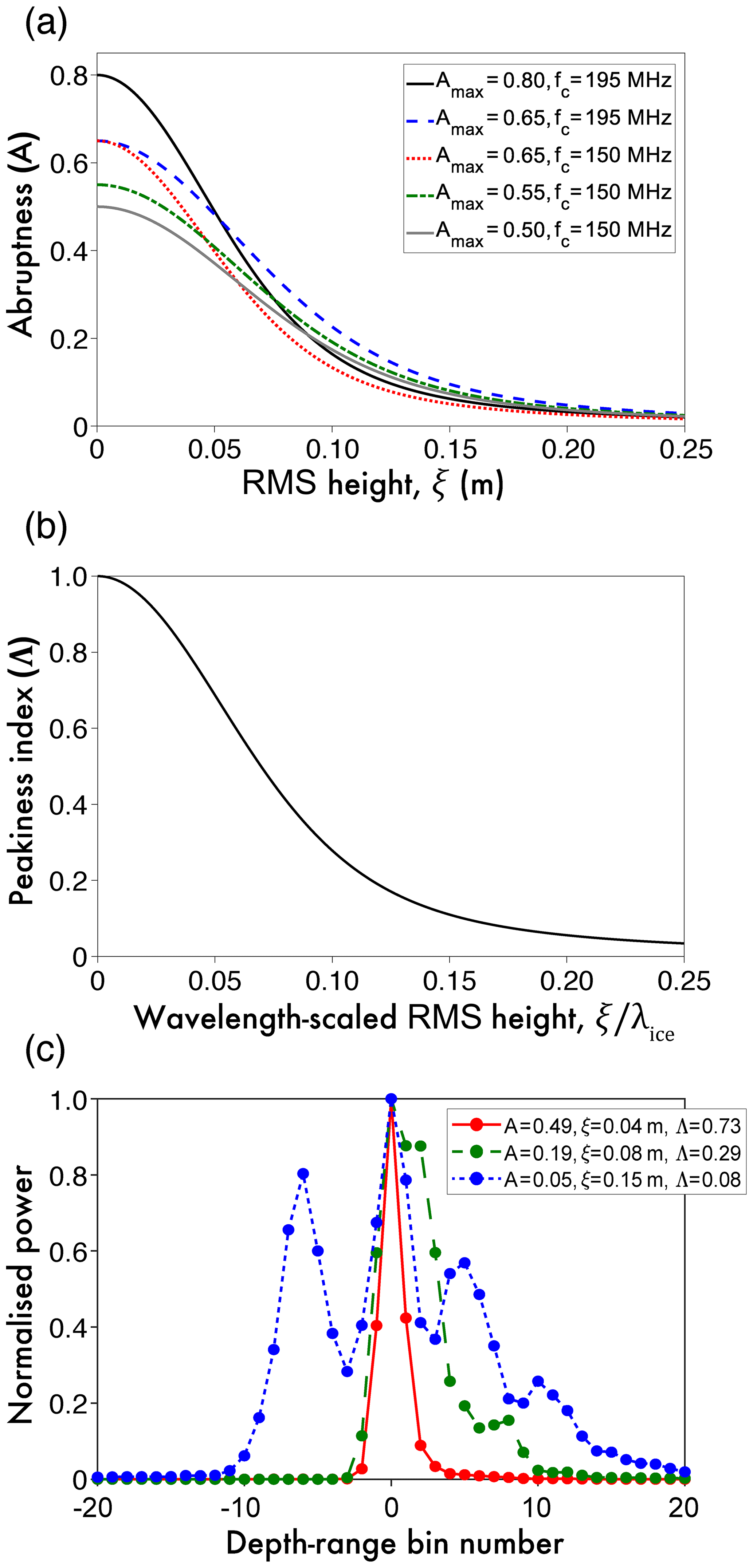
Figure 4Estimation of scattering-derived roughness and data combination for bed-echo peakiness. (a) Abruptness as a function of RMS height for different CReSIS field seasons: solid black curve – 2010 DC8; long dashed blue curve – 2011 TO, 2011 P3, 2012 P3, 2013 P3, and 2014 P3; dotted red curve – 2006 TO; dashed green curve – 2005 TO; and solid grey curve – 2008 TO and 2009 TO. (b) Peakiness index as a function of wavelength-scaled RMS height. (c) Example bed-echo waveforms, their abruptness (A), peakiness index (Λ), and scattering-derived roughness (ξ). The plots are for the 2011 P3 field season, which has maximum A∼0.65.
The procedure used to extract the bed-echo abruptness from CReSIS Level 1B data is outlined in Jordan et al. (2017). Briefly, this consists of the following three steps. First, CReSIS Level 2 picks are used as initial estimates for the depth-range bin of bed-echo power peak. Second, a local retracker is used to locate peak power. Third, the power is integrated over the bed-echo envelope, applying a “quality control” measure such that the peak power is 10 dB over the noise floor. This final step results in some regions, primarily in southern Greenland, having reduced coverage (see Fig. 1b in Jordan et al., 2018).
2.3.2 Estimating fine-scale roughness and the “peakiness index”
The scattering of the radar pulse at the glacier bed is underpinned by the physics of electromagnetic diffraction (Berry, 1973; Ulaby et al., 1982). As bed roughness increases, the radar pulse is scattered over a greater range of angles; this results in a decrease in peak returned power and an increase in the trailing edge of the echo. The mathematical formulation of this relationship depends on the physical model for electromagnetic interference (phase coherence or incoherence) and the statistical model for the subglacial interface (Berry, 1973; Peters et al., 2005; Haynes et al., 2018). The most commonly employed scattering model for the RES of glacier beds assumes phase-coherent interference, “smoothly undulating” Gaussian statistics for RMS roughness and radial isotropy (Berry, 1975; Peters et al., 2005; MacGregor et al., 2013; Grima et al., 2014; Schroeder et al., 2015). We employ this scattering model for two objectives: firstly as a way of estimating “fine-scale roughness” from the abruptness and secondly as a way of combining the abruptness for different radar systems to derive an (approximately) system-independent peakiness index (Λ).
Following a similar approach to that described by Schroeder et al. (2015) and Jordan et al. (2017), under assumptions of energy conservation, the scattering model can be used to predict the relationship between A and RMS height ξ (“fine-scale” roughness). In this context ξ is not strictly equivalent to the values obtained from topography, and a length-scale separation is performed with respect to a reference plane (Berry, 1973). The relationship between A and ξ is given by
where
denotes the RMS phase variation, with Amax being the maximum abruptness, I0 being a 0th-order Bessel function of the first kind, fc being the centre frequency of the radar pulse, c being the vacuum speed of the radar pulse, and ϵice=3.15 being the relative dielectric permittivity of glacier ice (Peters et al., 2005). Since the radar wavelength in ice is , Eq. (5) can be expressed as
and hence ξ is scaled by the radar wavelength in ice (either 0.87 or 1.13 m for the 195 and 150 MHz systems, respectively). There are therefore 2 degrees of freedom in Eq. (4) that can vary for different CReSIS field seasons: Amax and fc. The different parameter combinations are shown in Fig. 4a, and from these relationships it is possible to estimate ξ from A (and thus obtain a measure of fine-scale roughness that is similar between different radar systems). However, since the values of fc and Amax differ between field seasons, a crossover bias is present for “raw” abruptness values. In order to combine abruptness data, we back-substituted the value of ξ to obtain the value of A as if it were the most spatially extensive radar system (the blue curve in Fig. 4a) and then linearly rescaled amplitude on the interval [0,1] (using A∕Amax) to give the peakiness index (hereafter referred to as Λ). These steps combine the measurements via the system-independent relationship that is modelled between Λ and wavelength-scaled RMS height ξ∕λ (Fig. 4b).
The inter-season data combination was validated by performing crossover analysis for ξ and Λ, with the allowed tolerance for the crossover bias set to 5 % of the parameter range. RES data that do not meet this criterion (primarily the older ICORDS data but also the data from 2010 P3 season, which is known to have noise-floor issues; Paden, 2017) were discounted completely from analysis. Although the data combination scheme employed here, across CReSIS platforms, is seen to work well, it should be noted that combining data from multiple instruments, particularly those with a large difference in centre frequencies, may not be so effective.
It is important to note that obtaining ξ from Eq. (4) is just one way of estimating fine-scale roughness. Self-affine (fractal) statistics (Shepard and Campbell, 1999) can also be applied to scattering models of glacier beds (as in Jordan et al., 2017). Additionally, in reality, fine-scale roughness is anisotropic, as revealed by the “specularity” scattering metric (Schroeder et al., 2013, 2014, 2015; Young et al., 2016). We therefore recommend that ξ should be interpreted in a qualitative manner, with lower values indicating “fine-scale smooth” and higher values indicating “fine-scale rough” regions of the glacier bed. In regions of complex bed topography, and in particular at outlet glacier regions, off-nadir scattering may adversely influence the signal and lead to a breakdown in the interpretation of this metric (see Sect. 4.4). Fine-scale roughness that relates to radar scattering can also be estimated from the statistical distribution in peak bed-echo power (Neal, 1982; Grima et al., 2014).
3.1 Spatial distributions for subglacial roughness
3.1.1 Topographic roughness, R
Across the ice sheet, unfiltered (with respect to surface flow direction) R shows clear spatial heterogeneity (Fig. 5a); coherent signals, representing contiguous regions of both “smooth” (low R values) and “rough” (high R values) beds, are visible. Generally, the margins of the ice sheet contain the roughest beds, whereas the interior is notably smooth. Ice-sheet-wide, the lowest values of R are observed in the north and north-west of the island. However, localised to the main “trunks” of Petermann and Humboldt glaciers (PG and HG, respectively, in Fig. 5a), at the point of highest immediately before the grounding line, small patches of smooth bed are observed. Broadly speaking, across the ice sheet, fast-flowing regions exhibit rough beds; though, as exemplified in the north and north-west, this behaviour is somewhat spatially variable at the perimeter of Greenland. Notable examples of contiguous smooth beds near the margins include the following: north-west of the Camp Century (CC) drilling site, in the vicinity of Ìngia Isbræ (II; north of Rink Isbræ), and a region near the outlet of the North East Greenland Ice Stream (NEGIS; as marked in Fig. 5a). The highest values of R trace the Caledonian fold belt mountain range (formed in ∼420 Ma ago; Henriksen, 2008) and the deep inland fjord-like systems along the eastern and south-eastern margins of the island (Fig. 5a).
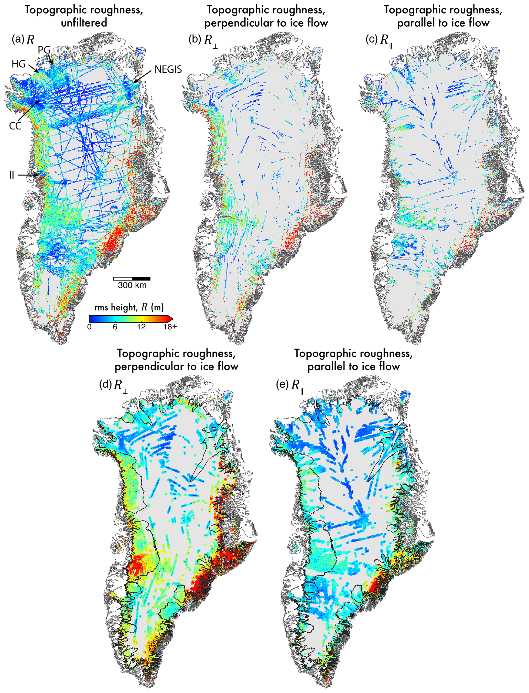
Figure 5Topographic roughness (R) across the GrIS. (a) R unfiltered by flow direction. (b) R⟂. (c) R∥. (d) and (e) show spatial interpolation of (b) and (c) to a width of 20 km, respectively, for improved visualisation. Locations for Ìngia Isbræ (II), NEGIS, Petermann Glacier (PG), Humboldt Glacier (HG), and Camp Century (CC) drilling site, as referred to in the text, are marked.
Figure 5b and c present directionally filtered values for topographic roughness, aligned perpendicular (R⟂) and parallel (R∥) to ice surface flow direction, respectively. For improved visualisation (and visual analysis) only, maps for R⟂ and R∥ were interpolated (using inverse-distance weighting) to a limit of 10 km (Fig. 5d and e). This interpolation distance is representative of the average track spacing used in the “gridded” airborne sampling regimes in fast-flowing regions (e.g. surrounding Jakobshavn Isbræ – JI – and Petermann Glacier – PG; see Fig. 1). Initial comparison shows a marked difference between R⟂ and R∥, most notably in fast-flowing regions. Across the ice sheet, the bed is observed to be smoother parallel to flow. In the ice-sheet interior (where ma−1) the subglacial environment is mostly smooth in both directions (i.e. isotropic). However, in the south of the ice sheet we observe more distinct differences between R⟂ and R∥ values (see Sect. 3.2). Overall, R∥ exhibits more uniform roughness values across fast- and slow-flowing regions, particularly within the north and west, whereas R⟂ presents a notable difference between fast- (rough) and slow-flowing regions (smooth).
We observe a similar spatial distribution of unfiltered R (Fig. 5a) to those previously quantified for Greenland using an RMS residual technique (see Fig. 4 in Layberry and Bamber, 2001) and through a frequency-domain approach (FFTs) undertaken at a much larger length scale (3200 km; see Fig. 1 in Rippin, 2013); in these studies, general conclusions for a smooth interior and rough margin were made. Rippin (2013) additionally notes a localised smooth bed underlying the trunk of Petermann Glacier, whereas Layberry and Bamber (2001) note a smooth basin for both Humboldt and Petermann glaciers. However, as these studies do not filter with respect to surface flow direction, they do not reveal roughness anisotropy in R across the ice sheet.
3.1.2 Scattering-derived roughness, ξ
Figure 6a presents the spatial distribution of scattering-derived subglacial roughness, ξ, for the GrIS. As noted in Sect. 2.3, these values are inversely correlated to Λ (Fig. 6b) due to the scattering model relationship. The spatial distributions observed within scattering-derived roughness are broadly similar to those observed for unfiltered R, including a notable link between fast flow and high values of ξ (rougher beds). Regions that present the smoothest subglacial environments also reflect those mentioned above, notably the vicinity of the CC drilling site, a coherent patch south-east of Petermann Glacier, towards the outlet of the NEGIS, and at Ìngia Isbræ (marked in Fig. 6a). Low (smooth) values of ξ are also observed along the central ice divide. In contrast to measures of R, however, and concordant with the broad-scale relationship of ξ to , the fastest-flowing trunks of Humboldt and Petermann glaciers contain rougher beds (HG and PG, respectively, in Fig. 6a). Other differences between topographic and scattering-derived roughness include a corridor of high ξ extending south of Petermann Glacier and across the ice divide (see Fig. 6a) as well as a generally more “mixed” roughness behaviour in the ice-sheet interior.
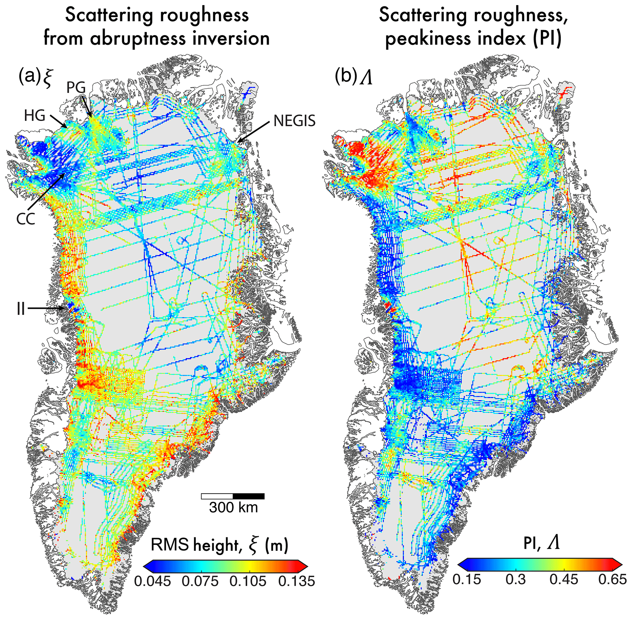
Figure 6Scattering-derived roughness (ξ) across the GrIS. (a) ξ. (b) Non-dimensional Λ (peakiness index) determined from the bed-echo waveform. Locations for Ìngia Isbræ (II), NEGIS, Petermann Glacier (PG), Humboldt Glacier (HG), and Camp Century (CC) drilling site, as referred to in the text, are marked.
3.2 Relationship with contemporary ice velocity
3.2.1 Ice-sheet scale
Owing to the isotropic nature of ξ, we limit more comprehensive assessment of the relationship between contemporary ice velocity and subglacial roughness to topographic roughness, R, only (undertaken using all calculated R bins). Figure 7 presents an assessment of the relationship between R with respect to surface ice flow direction in fast-flowing regions ( ma−1). The difference in distributions between R⟂ and R∥ (Fig. 7a and b) indicates that roughness perpendicular to flow direction is greater (i.e. more rough; mean is 9.39 m compared to 6.27 m) and exhibits higher variance (92.21 m2 compared to 43.02 m2).
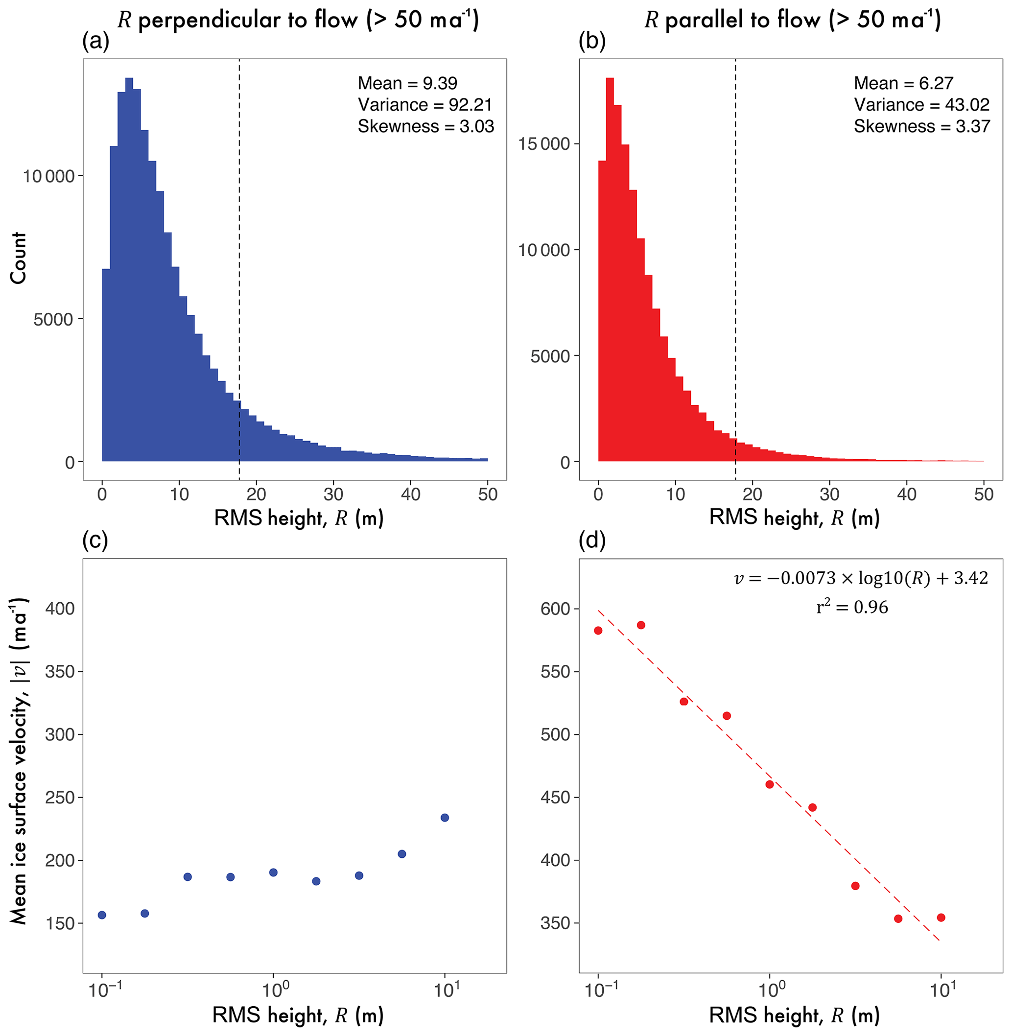
Figure 7Relationship between R⟂ and R∥ and surface ice velocity for fast-flowing ( 50 ma−1) regions of the GrIS. (a) and (b) present distributions R⟂ and R∥, respectively. (c) and (d) show mean ice surface speed, , calculations for logarithmic R bins (at 0.25 m intervals). This is a linear–log plot, where the limit of the horizontal axis (R) is 101.25 m, noted by the dashed black lines in (a) and (b). It should be noted that the vertical exaggeration of these two plots is constant. Mean values for ice surface speed are used here to facilitate direct comparability to previous work presented in Lindbäck and Pettersson (2015). Colours here are consistent with Fig. 3c for alignment with surface flow direction.
Calculated mean ice surface speeds () for logarithmic bins (at 0.25 intervals) of R⟂ and R∥ are shown in Fig. 7c and d, respectively. A marked difference between the calculated ice speed averages is observed. For all bins of R⟂, is seen not to exceed 250 ma−1, whereas the lower bound for , calculated for R∥, is >350 ma−1. This is most likely a result of a greater spread in values of for parallel roughness bins; however, it is notable that this scaling relationship is broadly in agreement with those previously observed in regional studies in Antarctica (Bingham and Siegert, 2007) and Greenland (Lindbäck and Pettersson, 2015). Additionally, if we are to assume that increases towards the glacier terminus (or grounding line), the exhibited scaling relationship for R∥ is in agreement with previous studies where roughness is observed to decrease (Bingham and Siegert, 2007, 2009). Increasingly smooth beds parallel to flow direction, therefore, are indicative of enhanced ice surface speed. The limit to which this relationship holds is R=101.25 (also delineated in distribution histograms by the dashed black line in Fig. 7a and b). This value is the approximate upper limit of R that can reasonably quantified using Eq. (1) (Sect. 4.4). Conversely, a weak positive relationship is observed between R⟂ and mean ice surface speed (Fig. 7c). R∥, however, exhibits a strong negative exponential scaling relationship with mean ice surface speed (Fig. 7d), which is statistically significant above the p=0.001 confidence level.
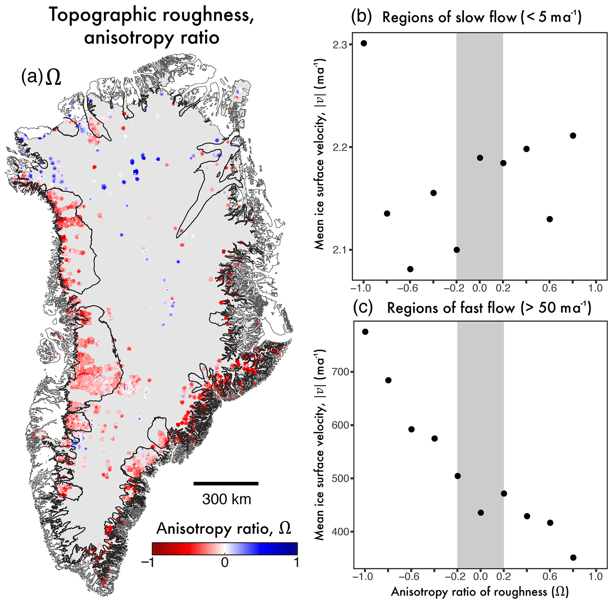
Figure 8Calculated anisotropy ratio for R. (a) Anisotropy ratio, Ω, where values of −1 dictate a dominance of smoothness parallel to flow direction, values of +1 indicate a dominance of smoothness perpendicular to flow (i.e., parallel roughness), and values of 0 indicate isotropy. (b) and (c) present mean ice surface speed, , calculated for anisotropy ratio bins (at 0.1 intervals) for slow- and fast-flowing regions, respectively.
Figure 8a presents the spatial relationship of the anisotropy ratio (Ω) across the ice sheet, where coincident values of R⟂ and R∥ are quantified. It is clear that fast-flowing outlet regions (the ice-sheet margins) are generally more smooth parallel to surface flow direction (where ). In the ice-sheet interior a more varied, or random, distribution in Ω is apparent. Mean ice surface speed for bins of Ω at 0.1 intervals, in fast- and slow-flowing regions (Fig. 8b and c), reinforces this observed spatial relationship in subglacial roughness. A strong linear relationship with regards to is exhibited within fast-flowing regions, whereas in regions of slow flow no such relationship is observed.
3.2.2 Fast-flow regions and outlet glaciers
To assess any spatial heterogeneity in the exponential scaling relationship between ice flow and R∥, local regions of fast flow were selected for closer analysis. These regions are centred around major outlet glaciers (Fig. 9) and, where possible, encompass only individual outlet glaciers (e.g. Humboldt – Region 1, Petermann – Region 2, and Kangerlussuaq – Region 4); however, where outlet glaciers are in close proximity, wider regions of fast flow were assessed (i.e. Jakobshavn+ – Region 6). Regionally, we observe the same exponential scaling relationship as exhibited ice-sheet-wide (see Fig. 10). The calculated regression line for each region is statistically significant at, or above, the p=0.01 confidence level, with the exception of Region 3 (encompassing NEGIS), at p=0.05. A marked difference in the regression gradients is also observed, spanning 4 orders of magnitude: Region 3 exhibits the shallowest gradient ( a−1), and Regions 4 and 5 exhibit the steepest gradient ( a−1 and a−1, respectively). Echoed by the shallow regression gradient and the lower confidence level of statistical significance, the NEGIS (Region 3) also exhibits the lowest r2 value (0.35). As previously described, both unfiltered R and ξ values reveal a contiguous smooth-bed signal, aligned near-perpendicular to flow direction (marked in Figs. 5a and 6a; further described in Sect. 4.1 and 4.3). Downstream from this, a coincident increase in subglacial roughness and is observed. Additionally, there is a notable sampling bias in the radar sounding across Region 3, where fewer tracks are aligned parallel to the flow direction (Figs. 3c and 9b). Together, these factors may be responsible for the weaker scaling relationship observed here between and R.
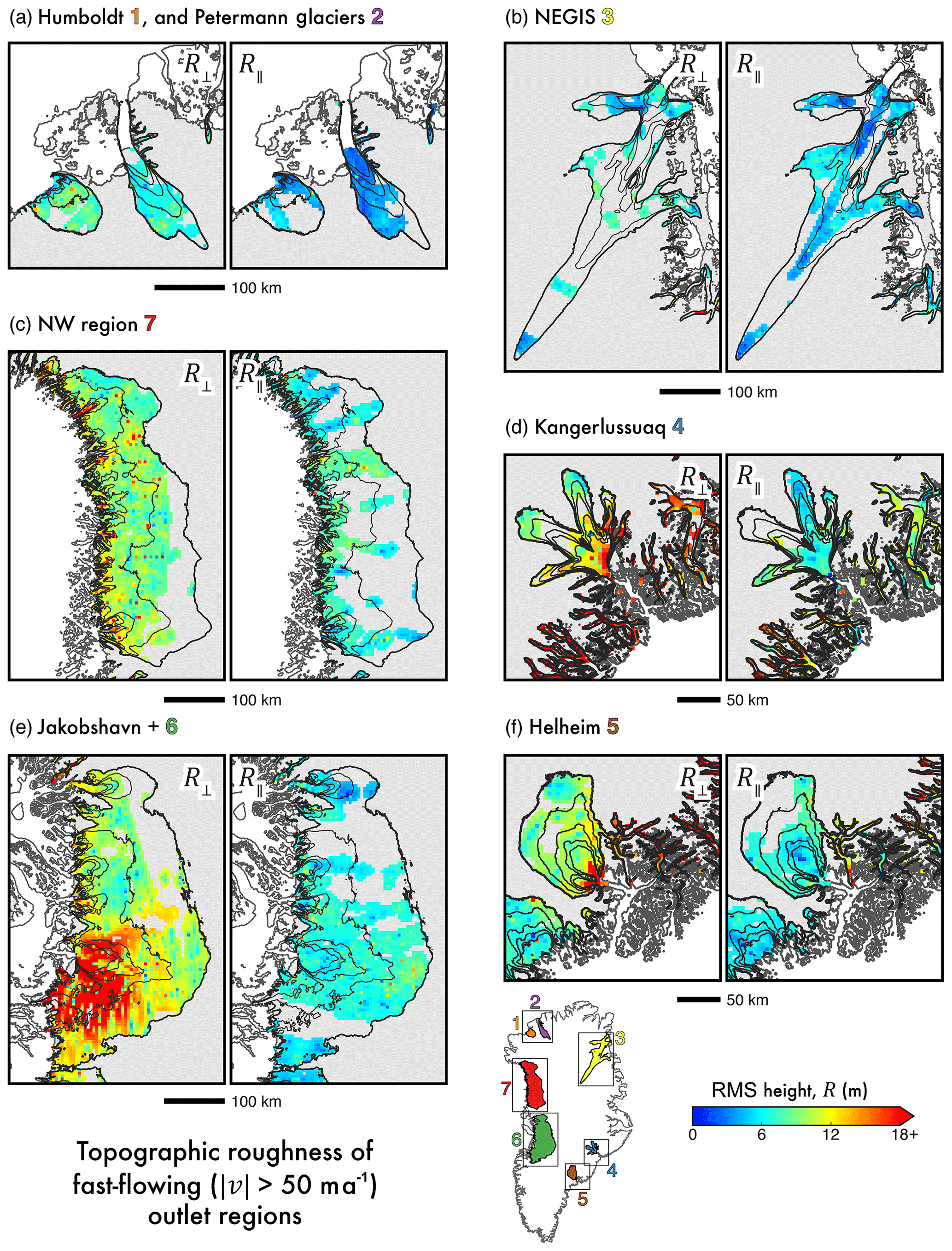
Figure 9Local subsets of R⟂ and R∥ in fast-flowing outlet glacier regions. Interpolated R⟂ and R∥ (as Fig. 5) are shown for the fast-flowing regions of (a) Humboldt (1) and Petermann (2) glaciers, (b) the North East Greenland Ice Stream (NEGIS; 3), (c) the north-western (NW; 7) fast-flow region, (d) Kangerlussuaq (4), (e) Jakobshavn Isbræ and surrounding glaciers (6), and (f) Helheim (5). The location of these regions is inset, where regions are colour-coded for further analysis (see Fig. 10).
More interestingly, two distinct groups are observed, showing a clear separation in regression slope gradients (Fig. 10). The first group (see bottom; Fig. 10) is mostly homogenous in terms of its regression slopes (i.e. the relationship between roughness and ice surface speed here is broadly similar). However, Region 4 and 5 in south-eastern Greenland (Kangerlussuaq and Helheim, respectively) exhibit a marked increase in gradient, indicative of a stronger scaling relationship at these sites.
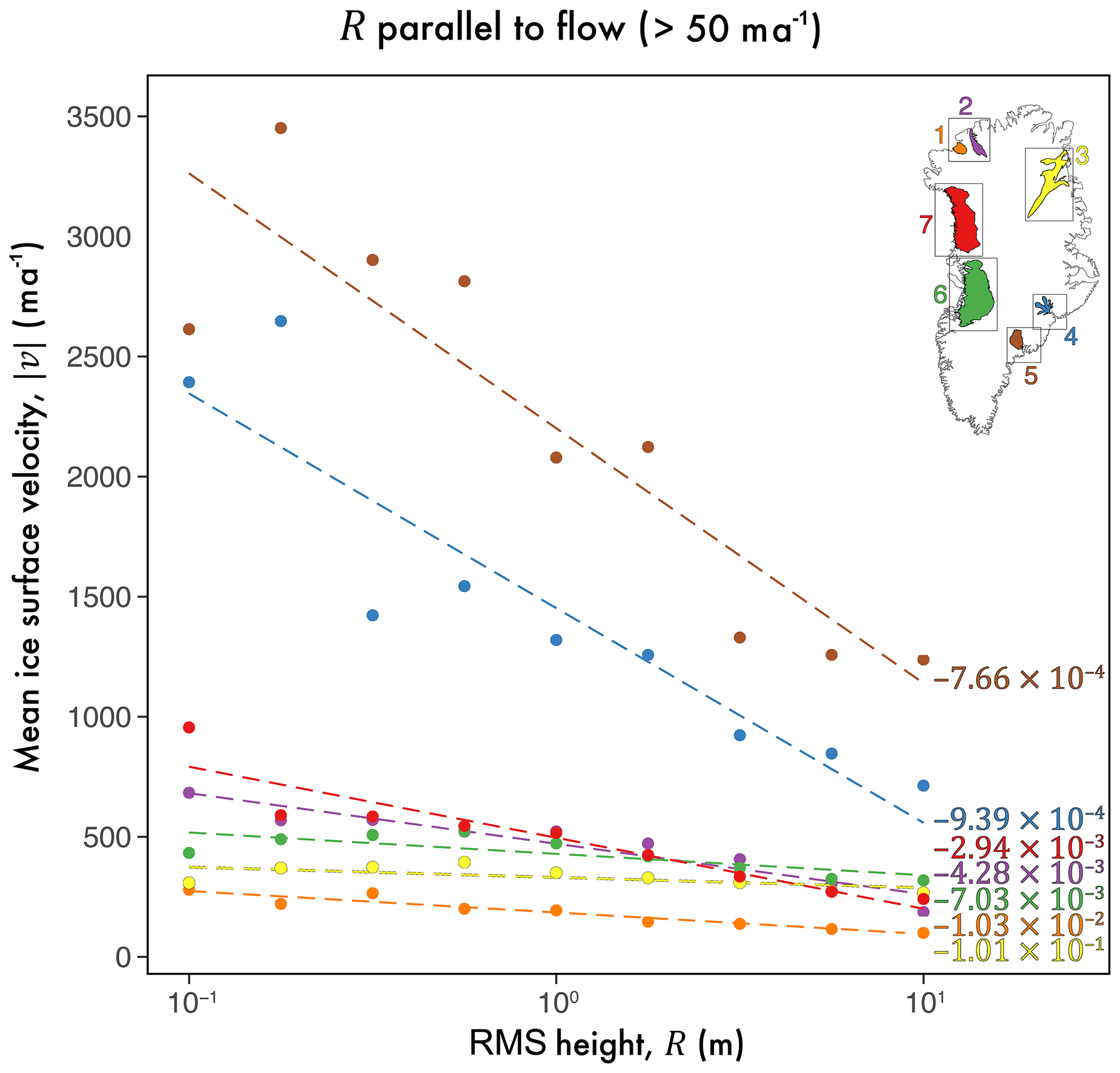
Figure 10Relationship between R∥ and ice surface speed for fast-flowing outlet glacier regions. This is a linear–log plot as per Fig. 7d, depicting the calculated mean ice surface speed, , for logarithmic R bins (at 0.25 m intervals) at each of the seven regions shown in Fig. 9; the gradient of the linear model (with units of a−1) for each region is shown in ascending order (less negative).
3.3 Contiguous smooth beds in slow-flowing regions
To recap, we observe coherent, contiguous “smooth” regions present across the GrIS across both roughness metrics (Figs. 5 and 6). These regions include north-western Greenland (around CC; Fig. 11), the region south-east of the Petermann Glacier (Fig. 12), and the region bisecting central Greenland bounded west and east by Ìngia Isbræ and Geikie Plateau, respectively (II and GP; Fig. 13). Owing to its isotropic nature, and inherent sensitivity to more-fine-scale roughness information, we focused on measures of ξ for these regions. High abruptness values (comparable to Λ; Fig. 4b) in several of these regions have previously been observed (e.g. Fig. 6c in Jordan et al., 2017; Oswald and Gogineni, 2012). For the most part, these are coincident with regionally high, and flat, beds (Morlighem et al., 2017), slow surface ice speed (Joughin et al., 2016), and a frozen basal thermal state (MacGregor et al., 2016; Jordan et al., 2017).
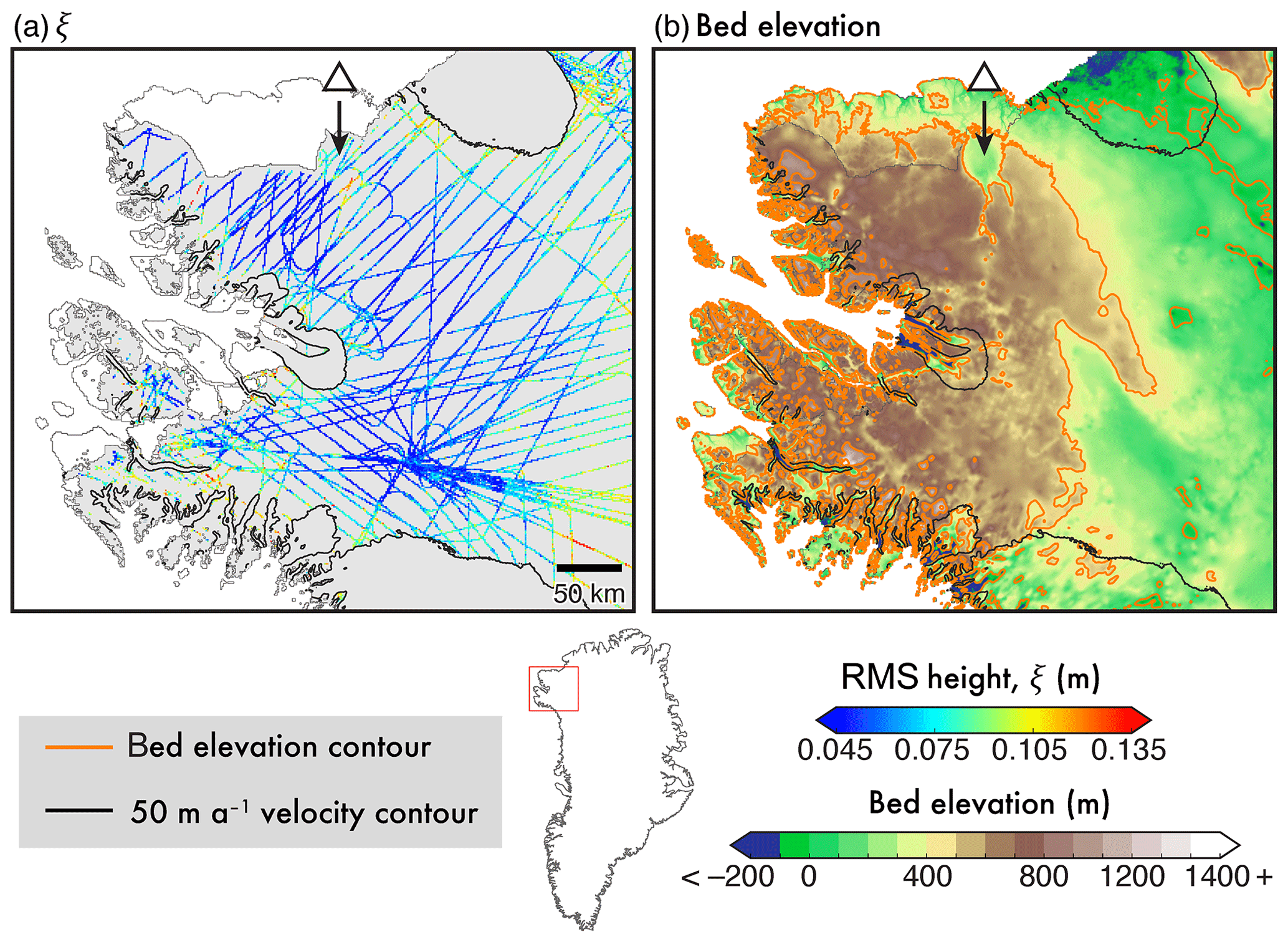
Figure 11Geological interpretation using scatting-derived roughness, ξ, near Camp Century. (a) ξ, with values in fast-flowing regions (delineated by black contour; ma−1) masked. (b) Bed elevation (BedMachine, v3; Morlighem et al., 2017) with contours at 400 m intervals. The site of the Hiawatha impact crater (Kjær et al., 2018), associated with channelised features is marked (triangle; discussed in Sect. 4.3). Location inset.
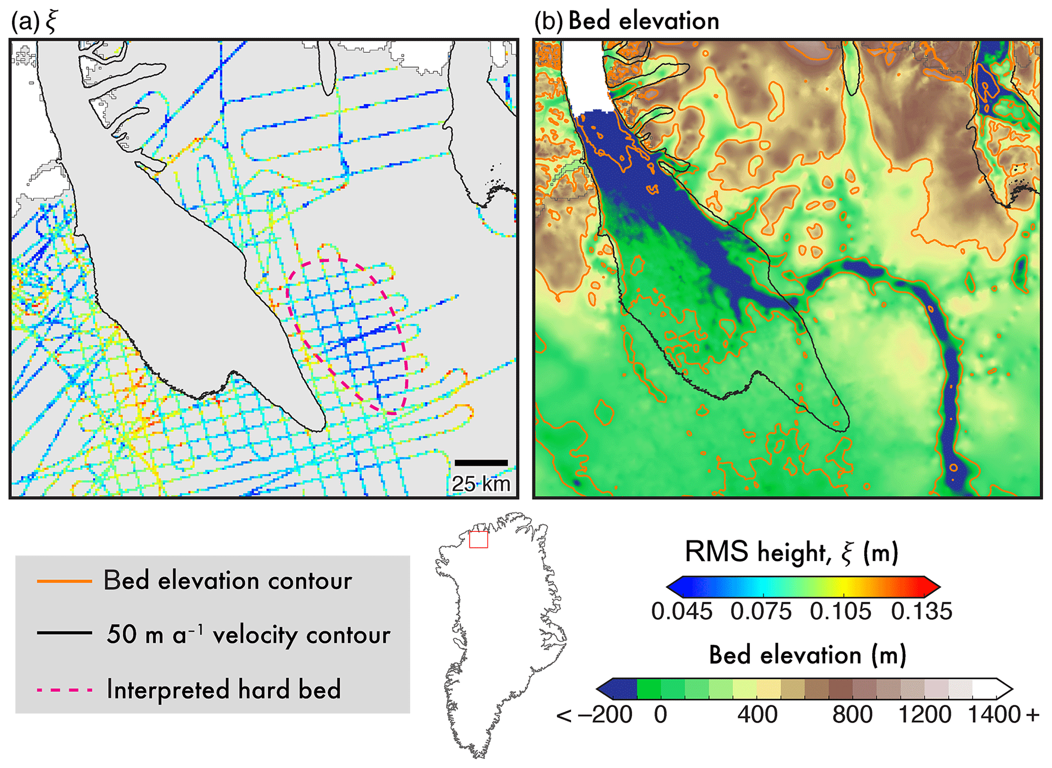
Figure 12Geological interpretation using scatting-derived roughness, ξ, at Petermann Glacier. (a) ξ, with values in fast-flowing regions (delineated by black contour; ma−1) masked. Interpreted hard bed delineated by pink dashed line. (b) Bed elevation (BedMachine, v3; Morlighem et al., 2017) with contours at 400 m intervals. Location inset.
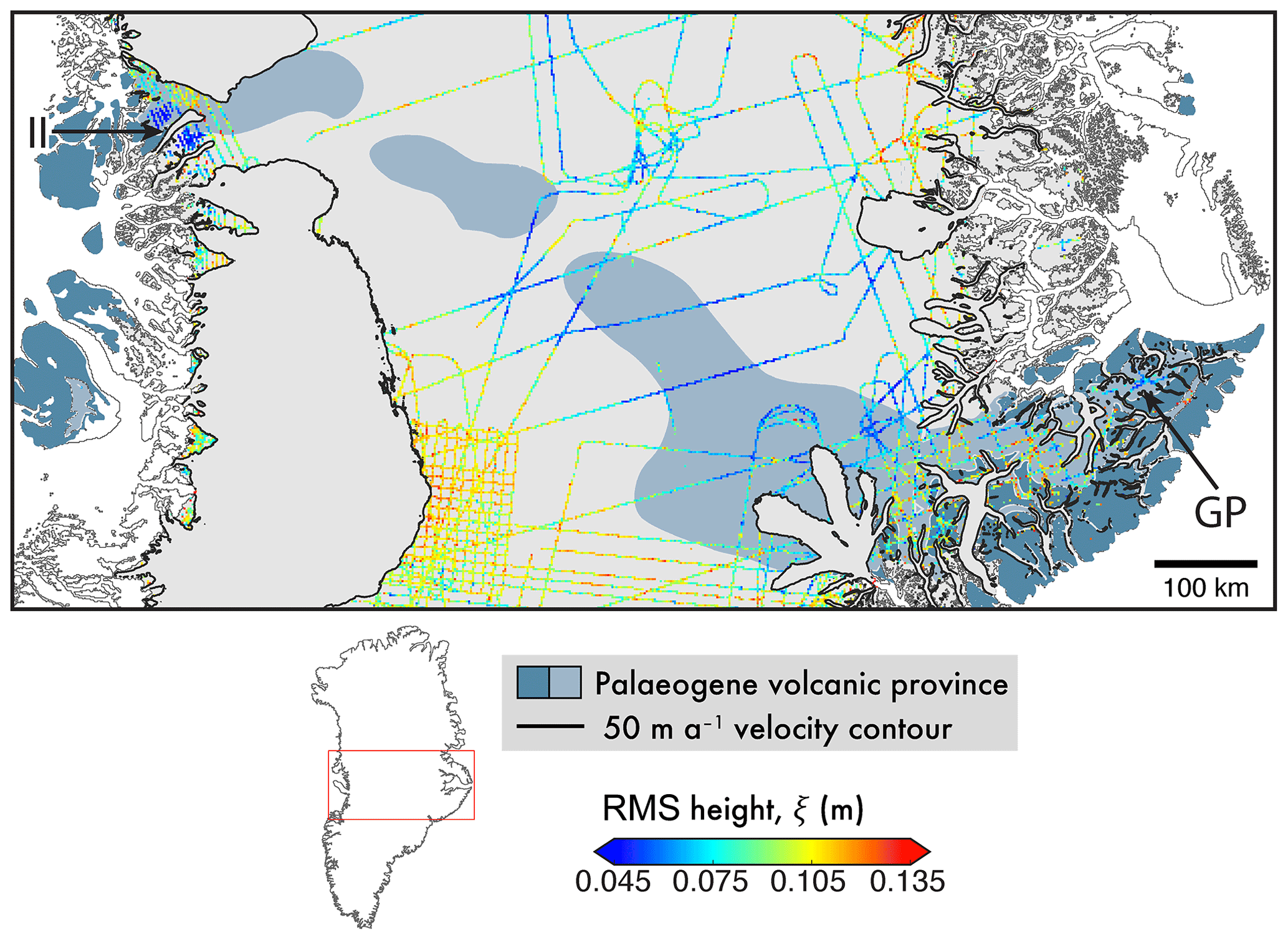
Figure 13Geological interpretation using ξ in central Greenland. Values of ξ in fast-flowing regions are masked (delineated by black contour; ma−1). Exposed or ice-free (dark shading) and predicted extent (light shading) of a Palaeogene volcanic province (Dawes, 2009) is underlain. This feature is bounded west and east by Ìngia Isbræ (II) and Geikie Plateau (GP), respectively. Location inset.
4.1 Interpretation of spatial patterns
As previously mentioned, Weertman-style hard-bed sliding laws are theoretically influenced by basal traction exerted on the ice column by small-scale basal obstacles (on the order of ∼1 m; Weertman, 1957; Nye, 1970; Durand et al., 2011). However, the most prevalent methods of quantifying subglacial roughness (i.e. through statistical analysis of along-track bed elevation, as in this study) are limited to evaluating basal information directly on the order of 100–1000 m or downscaled using fractal parameters (as in Jordan et al., 2017). Nevertheless, in regional studies of West Antarctica (e.g. the Siple Coast), a smooth bed has widely been considered a control on the location of fast-flowing, streaming ice (Siegert et al., 2004, 2016; Peters et al., 2006; Bingham and Siegert, 2009), and, in contrast, slow-flowing regions have been observed to widely exhibit more-rough beds (Siegert et al., 2004; Bingham and Siegert, 2007; Rippin et al., 2006, 2014).
However, when assessed across Greenland, it is evident that the spatial relationship between subglacial roughness and appears to be non-universal (in particular, fast-flowing regions can be both rough and smooth). In direct contrast, rough beds have been observed to be coincident with contemporary fast-flowing ice both in Antarctica (Schroeder et al., 2014; Bingham et al., 2017) and, previously, in Greenland (Rippin, 2013; Jordan et al., 2017). In this study, as exhibited across both unfiltered topographic roughness (R) and the more-fine-scale, scattering-derived roughness (ξ) measure, a similar spatial relationship to is observed (Figs. 5a and 6a). Rough beds are seen to dominate fast-flowing regions, where slow-flowing regions are predominantly smooth. Whilst this relationship does not necessarily appear to conform to the classical interpretation that smooth beds are a necessary condition for fast flow, it is important to note that the length scale used in this study, at least for R (200 m), is too coarse to identify roughness information that is pertinent to basal traction and, by extension, Weertman-style hard-bed sliding laws. Theoretically, scattering-derived roughness is sensitive to roughness information at, or between, the scale of radar wave length (on the order of ∼1 m) and that of the Fresnel zone (on the order of ∼100 m; Shepard and Campbell, 1999) and, therefore, may provide useful insight with respect to the influence of small-scale obstacles on basal sliding; however, without a more rigorous understanding of the scale separation (later discussed in Sect. 4.4), it is not possible to use this metric to parameterise basal friction in a general way across the ice sheet. Additional interpretation of the relationship between subglacial roughness, namely flow-filtered topographic roughness (R⟂ and R∥), and is given below (Sect. 4.2).
Where a direct influence on basal traction has proven elusive in previous research, the interpretation of subglacial roughness has centred on geomorphic means. One such framework is outlined by Bingham and Siegert (2009), whereby smooth-bedded regions have been associated with the presence of deformable sediment, perhaps attributable to marine sedimentation (e.g. Rippin et al., 2006, 2011, 2014; Bingham and Siegert, 2007) or as a result of enhanced erosion resulting in topographic streamlining within bedrock (e.g. Siegert et al., 2005; Rippin et al., 2014). Low-lying topographic basins, particularly within a marine setting, may promote a smooth bed owing to marine deposition (sedimentation) during deglaciated periods (Bingham and Siegert, 2009). In this vein, the localised, relatively smooth bed observed underlying NEGIS may be a likely candidate for deformable sediment (marked in Figs. 5a and 6a) and, documented in Christianson et al. (2014), characterises the presence of subglacial till in this region through seismic analysis; this is coincident with a marine overdeepening underlying NEGIS as well as low R and ξ values (smooth beds) as quantified in this study (Figs. 5a and 6a). More in-depth assessment of the presence of sediment, alongside the evaluation of hard (non-deformable) beds, is further discussed below (Sect. 4.3).
Much of the ice-sheet interior is characterised by a frozen basal thermal state (MacGregor et al., 2016), which, alongside low , suggests that rates of erosion or sediment transport (deposition) is negligible. Smooth beds in regions of slow flow have previously been characterised as markers of palaeo-ice streams, or fast flow, in regional Antarctic studies (e.g. Siegert et al., 2005; Bingham and Siegert, 2009; Lindbäck and Pettersson, 2015). Whilst such an interpretation of the smooth-bedded interior across Greenland (Figs. 5a and 6a) is not feasible for the modern ice sheet, it may be plausible to attribute this to the topographically unconstrained waxing and waning of the GrIS over multiple interglacial cycles (allowing for widespread glacial scour; Sugden, 1974).
4.2 Interpretation of roughness–velocity scaling relationships
As noted above, the consideration of orientation within subglacial-roughness interpretation is important (Gudlaugsson et al., 2013; Falcini et al., 2018) despite previously being limited to regional studies (e.g. Bingham and Siegert, 2007; Lindbäck and Pettersson, 2015). Analysis of flow-filtered R values demonstrates a pronounced anisotropy of the subglacial roughness. This is not only observed ice-sheet-wide at crossover measures via the anisotropy ratio (Ω; Fig. 8) but also in the marked difference in roughness behaviour in fast-flowing regions ( ma−1; Fig. 7). Distributions of R⟂ and R∥ values suggest that the subglacial environment of Greenland is not only more smoothly aligned parallel to flow direction on average but that R∥ tends towards smaller values (Fig. 7a and b), giving rise to different relationships between and R⟂ and R∥ (Fig. 7c and d, respectively).
As the length scale of R is too great to directly relate to basal traction within a Weertman-style hard-bed sliding law (Weertman, 1957; Nye, 1970), a different interpretation must be made with reference to the exhibited roughness–velocity scaling relationships. As such, increasing is unlikely to be explained by a decrease in R∥ values; this change is more likely attributable to enhanced erosion or sediment transport (increasing with ), resulting in a streamlining (or elongation) of bed features, possibly within deformable sediment (e.g. mega-scale glacial lineations – MSGLs – observed in King et al., 2009; Schroeder et al., 2014; Bingham et al., 2017). Additionally, the positive, albeit weak, relationship between and R⟂ could be plausibly explained by enhanced erosion increasing cross-feature amplitude (greater R⟂ values) of streamlined beds. Generally, the spatial distribution of R⟂ values presents a more marked difference between fast- and slow-flowing regions when compared to values of R∥. This is most likely influenced by velocity-controlled bed morphology, including both large-scale troughs and linear bedforms, such as MSGLs.
The roughness–velocity scaling relationship observed parallel to the flow direction is seen to be locally variable (Fig. 10). The likely cause for the clear separation, or “grouping”, within the regression gradients is likely due to the nature of the underlying topography. Kangerlussuaq (Region 5) and Helheim (4) glaciers are classically defined as being “topographically constrained”, where flow is steered to the margin through steep-sided troughs. This influences the onset of flank flow, providing more lateral control to fast-flowing ice and its basal motion, impacting local rates of erosion and/or deposition. Although Jakobshavn Isbræ is also considered to be topographically constrained, we do not see such a pronounced relationship for the Jakobshavn+ region (Region 6; Fig. 10). This is likely because we have conglomerated neighbouring glaciers due to their spatial density; however, this does suggest that topography provides less lateral control in this region, as stated by Rippin (2013).
4.3 Interpreting hard-bed geology
In fast-flowing regions ( ma−1), we observe mixed behaviour in subglacial roughness. Parallel to ice flow direction (R∥), smooth beds are a likely a result of enhanced erosion controlled by , whereas isotropic measures exhibit rough beds (high values of ξ and R) coincident with fast-flowing regions (Sects. 3.2 and 4.2). However, it is clear that fast flow is not a necessary condition for low roughness values (Figs. 11–13). Where ice motion is thought not to be driven by basal sliding (in regions of slow flow), a condition largely controlled by basal thermal state, rates of basal erosion are limited (van der Veen, 2013; MacGregor et al., 2016). It is, therefore, in these regions where we consider an alternative “control” with regards to low ξ and R values (smooth beds), further elucidating characteristics of the subglacial environment.
High waveform abruptness (A) values, here normalised across radar sounders as Λ, have, when combined with radar bed-echo reflectivity, been used to discriminate the basal thermal state where larger, contiguous regions have been associated with bodies of, electrically deep, water (Oswald and Gogineni, 2008, 2012; Oswald et al., 2018). However, recent comparison alongside ice core temperature data and a synthesis for the likely basal thermal state (MacGregor et al., 2016) in north-western Greenland shows this relationship to be largely inconsistent, particularly at the spatial scales (extent) assessed here (e.g. Fig. 6; Jordan et al., 2017). To build upon Jordan et al. (2017), we integrate existing knowledge of bed geology (Dawes, 2009) and information from complementary geophysical surveys (i.e. gravity and magnetic anomalies; Tinto et al., 2015) to highlight that low values of ξ may indeed indicate a hard bed, particularly in large, contiguous regions (>1000 km2). Due to the impermeability of igneous rocks, however, low values of ξ may also be a result of increased water at the ice–bed interface, giving rise to increased specularity in reflected bed echoes (high Λ).
4.3.1 Camp Century
Figure 11 presents one such contiguous region of smooth beds in the vicinity of the CC drilling site: where an increase in ξ is observed towards the east and south-east, near Humboldt Glacier. Fast-flowing regions have been masked, owing to the isotropic nature of scattering-derived roughness and the anisotropic behaviour of topographic roughness outlined above (Sect. 3.2). As the bed is likely frozen in this region (MacGregor et al., 2016), where we also observe a high elevation plateau and slow-flowing ice (and a local ice divide), it is not feasible to interpret this signal as simply the presence of electrically deep basal water. From the knowledge, albeit limited, of subglacial geology in this region (see Fig. 1 in Dawes, 2009), we propose that this signal (of low ξ) is in fact caused by a non-deformable bed, related to underlying geology on which there is little to no sediment. This bed, reminiscent of preglacial erosion surfaces observed in Antarctica (Rose et al., 2015), is also likely to have been largely untouched by long-term glacial erosion.
Also observed in this region are elevated ξ values coincident with the Hiawatha impact crater (Kjær et al., 2018), associated with channelised features (triangle; Fig. 11). Whilst higher values of ξ may well be due to the interference from off-nadir echoes (as explained above; see Sect. 4.4), it is plausible that, by contrast, this may be a marker for a soft bed (i.e. presence of deformable sediment), as a result of enhanced sediment transport.
4.3.2 Igneous intrusion, Petermann Glacier
Figure 12 depicts scattering-derived roughness and bed elevation near Petermann Glacier, north-west Greenland. East of the streaming ice and bounded to the north and east by the palaeo-fluvial “mega-canyon” (Bamber et al., 2013), we observe a contiguous low-ξ region where surface flow speed is <50 ma−1. This signal is observed coincident with a local topographic high (with a prominence of 300 m in elevation), which, unlike the surrounding topography, is largely left unmarked or dissected by bed channels. Previous geophysical interpretation, using both gravity and magnetic anomalies derived from OIB data (see Fig. 2 in Tinto et al., 2015), has established this unit as an intruded igneous body. The unaltered nature, and geological interpretation, of this feature further lend credibility to our interpretation of low ξ values as denoting a hard bed. Additionally, recent assessment of the basal thermal state, and basal water prediction derived from RES, suggest that this region is not predominantly “wet” (MacGregor et al., 2016; Jordan et al., 2018; Chu et al., 2018), further indicating that the interpretation of water ponding is unlikely to hold here.
4.3.3 Volcanic province, central Greenland
Well-constrained by exposed geology at the ice-free margins of Greenland (bounded west and east by Ìngia Isbræ and Geikie Plateau, respectively) is the presence of a volcanic province from the Palaeogene (Fig. 13; see also Fig. 1 in Dawes, 2009) under the inland ice in central Greenland. However, the exact extent of the presence of the underlying basaltic rocks cannot be accurately determined (Dawes, 2009). At each margin of the GrIS where is <50 ma−1, we see good spatial agreement between ξ and the mapped volcanic province. If we are to conclude that low values of ξ delineate a hard bed, it may be possible to redraw the boundary of the volcanic province further inland from the western margin (Fig. 13). The eastern end of this “smooth” region is spatially correlated with elevated levels of geothermal heat as a result of the long-term tracking of the Icelandic hotspot, a relatively thin lithosphere, and an underplated body, discussed by Rogozhina et al. (2016) and Martos et al. (2018).
4.3.4 Delineating deformable and non-deformable beds
In many assessments of subglacial roughness in Antarctica, smooth beds have been associated with the presence of weak sediment layers beneath fast-flowing outlet glaciers (e.g. Bingham and Siegert, 2009; Rippin et al., 2014; Bingham et al., 2017) (Sect. 4.2), whereby the deformation of this sediment does not only exert important spatial controls upon the onset of fast flow but also upon ice speed in Antarctica (Alley et al., 1986; Peters et al., 2006; Siegert et al., 2016) and potentially in Greenland (Bougamont et al., 2014; Stearns and van der Veen, 2018). It is clear, however, from the regions previously described, that fast flow is not a necessary condition for large, coherent regions of “smooth” bed. Where basal conditions are not indicative of enhanced ice flow (i.e. slow-flowing, cold-based regions), we suggest that low values of ξ are indicative of a non-deformable, hard bed. However, this will only work well away from complex terrain (i.e. regions of low relief; see Sect. 4.4). Although we reject that such contiguous signals as are evidence of ponded basal water, or indeed basal thaw, it is plausible that small-scale patches of high abruptness values (high Λ and low ξ values) could still be interpreted this way.
If we extend our conclusion that ξ may be used to demarcate underlying hard beds, focus should then be drawn to regions where deforming basal sediment and sediment transport is likely to take place. As discussed, the majority of fast-flowing outlet regions exhibit high values of ξ (Fig. 6a; unfiltered R – Fig. 5a), which, by R∥, we interpret as exhibiting basal “streamlining” influenced by (akin to that observed by Bingham et al., 2017, albeit at a different scale). This, alongside recent evaluation that states that many of Greenland's outlet glaciers may be driven by the availability of basal deforming sediment (Bougamont et al., 2014; Stearns and van der Veen, 2018), suggests that high values of ξ are a proxy to demarcate deformable beds.
4.4 Roughness scale separation and breakdown in complex terrain
As the quantification of topographic roughness (R) uses a defined length scale (L=200 m), the interpretable scale of subglacial-roughness information, and the roughness “feature”, is fixed at this order of magnitude; however, understanding the scale of information provided by scattering-derived roughness (ξ), and the scale separation between both roughness measures, is likely to be variable across the ice sheet. As previously mentioned, scattering-derived roughness is sensitive to roughness information between ∼1 and 100 m (Shepard and Campbell, 1999). However, as the observed spatial distribution of ξ is seen to be broadly similar to that of unfiltered R (Figs. 5a and 6a, respectively), it may be reasonable to suggest that this measure (scattering-derived roughness) may be more appropriately interpreted as defining roughness characteristics at the larger scale.
Local topography ultimately leads to the breakdown of both subglacial-roughness metrics presented here but also likely affects the degree of scale separation across the ice sheet. Notably, this occurs where a large step change is observed in bed elevation (“cliff-like” regions; i.e. deep subglacial troughs). Here, bed-echoes are likely to exhibit more diffuse waveform characteristics due to off-nadir echoes from the valley sides; these will present erroneously high values of ξ (a “false” rough ice-bed interface), thus adversely affecting interpretation. For this reason, it may be sensible to use quantified values of topographic roughness to infer whether values of ξ are providing useful information. For example, if coincident measures of R and ξ are low (topographically smooth) and high, respectively, it may be clear that the subglacial environment is exhibiting more-fine-scale roughness information.
Additionally, it is important to note that measures of R also break down in similarly complex terrain, where cliff-like changes in along-track bed topography fall within the sampling window. An example of this is illustrated by the transparent grey bars in Fig. 2. Both metrics, however, assume a Gaussian distribution about a mean surface; where local topography exhibits such step changes, it appears that this statistical model for roughness no longer holds. As such, the main conclusion we draw in this study with regard to R and ice-sheet motion remains unaffected, as the exponential scaling relationship (Fig. 7d) holds for the lower end of R∥ values (), accounting for the vast majority of calculated values in fast-flowing regions.
We have presented the first systematic approach to quantifying and comparing subglacial roughness across the GrIS using two independent methods at differing length scales: statistical analysis of topography and the properties of the bed-echo waveform (scattering). This not only provides an updated “map” for the spatial distribution of subglacial-roughness characteristics in Greenland (cf. Layberry and Bamber, 2001; Rippin, 2013) but further quantifies the relationship between roughness and ice-sheet motion. The study also helps with elucidating other spatially heterogenous aspects of the subglacial environment. For our measure of topographic roughness (R), we have provided near-complete spatial coverage, making use of data from all publicly available CReSIS radar sounding campaigns (1993–2016). Filtering R with respect to surface ice velocity (i.e. speed and direction) has enabled the assessment of roughness anisotropy both at the ice-sheet-scale and more locally in certain regions and at specific outlet glaciers.
Values for subglacial roughness, quantified here using both topographic- and scattering-derived metrics, suggest that the majority of fast-flowing outlet glaciers are underlain by rough beds. Conversely, the slow-flowing interior is smooth. A pronounced anisotropy in topographic roughness with respect to ice flow direction is evident, particularly in fast-flowing regions ( ma−1), whereby R exhibits an exponential scaling relationship with ice surface speed parallel, but not perpendicular, to flow direction. We therefore suggest that consideration of roughness anisotropy is required with a view to inferring relationships with ice motion and subglacial processes. Whilst it is inappropriate to make any conclusions that the wavelengths of roughness information quantified in this study induce basal traction (with reference to a Weertman-style hard-bed sliding law), further interpretation of the spatial variation in scale sensitivity of scattering-derived roughness may well provide some information for basal traction parameterisation at a local scale. For topographic roughness (where L=200 m) the observed anisotropy and scaling relationships observed are likely due to enhanced rates of subglacial erosion resulting in a streamlining of bed features, possibly through deforming basal sediment (e.g. MSGLs observed in King et al., 2009; Schroeder et al., 2014; Bingham et al., 2017). Additionally, in many regions of slow flow, we conclude that contiguous areas of smooth beds (as quantified by ξ) are likely due to the presence of a hard bed rather than the presence of soft, deformable sediment.
The two subglacial-roughness metrics presented here are available for download from the Polar Data Centre, Natural Environmental Research Council, UK, at https://doi.org/10.5285/6071926f-32e0-4681-a50d-aab08f42c08a (Cooper et al., 2018). The Level 1B and Level 2 RES data are available from CReSIS at https://data.cresis.ku.edu/data/rds/ (last access: September 2018) and are documented in Paden (2017). The Greenland basal thermal-state synthesis (MacGregor et al., 2016), ice thickness and topography data sets (BedMachine, V3; Morlighem et al., 2017), and ice surface speed (Joughin et al., 2016) are archived by NSIDC at https://doi.org/10.5067/R4MWDWWUWQF9, https://nsidc.org/data/idbmg4 (last access: September 2018), and https://nsidc.org/data/ NSIDC-0670/versions/1 (last access: September 2018), respectively.
This study was initiated by JLB and co-advised by MJS as part of the Basal Properties of Greenland Project. MAC wrote the paper, with support from TMJ; together, they analysed the radar data with processing advice from DMS. CNW assisted in geospatial problem-solving with regards to radar processing. All authors commented on drafts of the manuscript and contributed to the interpretation of the science.
JLB is the advisory editor of The Cryosphere. The authors declare that they have no conflict of interests.
In addition to the financial support received, listed below, which supported Michael A. Cooper, Thomas M. Jordan, Martin J. Siegert, Christopher N. Williams, and Jonathan L. Bamber, Dustin M. Schroeder was supported by a grant from the NASA Cryospheric Sciences Program. We would like to thank John Paden, CReSIS, for their advice on radar data processing, and we acknowledge the use of data products from CReSIS generated with support from NASA grant NNX16AH54G. Additionally, we thank Rob Bingham for useful comments on an earlier version of this paper; of course, we give special thanks to Poul Christoffersen and the anonymous referee for their constructive feedback in reviewing this work and Olivier Gagliardini, as the editor, for their handling of this paper.
This research has been supported by the Natural Environment Research Council (grant no. NE/L002434/1), the Natural Environment Research Council (grant no. NE/M000869/1), and EU Horizons 2020 (grant no. BRISRES (747336)).
This paper was edited by Olivier Gagliardini and reviewed by Poul Christoffersen and one anonymous referee.
Alley, R. B., Blankenship, D. D., Bentley, C. R., and Rooney, S. T.: Deformation of till beneath ice stream B, West Antarctica, Nature, 322, 57–59, https://doi.org/10.1038/322057a0, 1986. a, b
Arthern, R. J., Hindmarsh, R. C. A., and Williams, C. R.: Flow speed within the Antarctic ice sheet and its controls inferred from satellite observations, J. Geophys. Res.-Earth Surf., 120, 1171–1188, https://doi.org/10.1002/2014JF003239, 2015. a
Bamber, J. L., Siegert, M. J., Griggs, J. A., Marshall, S. J., and Spada, G.: Paleofluvial mega-canyon beneath the central Greenland Ice Sheet, Science, 341, 997–999, https://doi.org/10.1126/science.1239794, 2013. a
Berry, M. V.: The statistical properties of echoes diffracted from rough surfaces, Philos. Trans. Roy. Soc. London A, 273, 611–654, https://doi.org/10.1098/rsta.1973.0019, 1973. a, b, c, d
Berry, M. V.: Theory of radio echoes from glacier beds, J. Glaciol., 15, 65–74, https://doi.org/10.3189/S0022143000034274, 1975. a
Bingham, R. G. and Siegert, M. J.: Radar-derived bed roughness characterization of Institute and Möller ice streams, West Antarctica, and comparison with Siple Coast ice streams, Geophys. Res. Lett., 34, L21504, https://doi.org/10.1029/2007GL031483, 2007. a, b, c, d, e, f, g, h, i
Bingham, R. G. and Siegert, M. J.: Quantifying subglacial bed roughness in Antarctica: implications for ice-sheet dynamics and history, Quaternary Sci. Rev., 28, 223–236, https://doi.org/10.1016/j.quascirev.2008.10.014, 2009. a, b, c, d, e, f, g, h, i, j, k, l, m
Bingham, R. G., Siegert, M. J., Young, D. A., and Blankenship, D. D.: Organized flow from the South Pole to the Filchner-Ronne ice shelf: An assessment of balance velocities in interior East Antarctica using radio echo sounding data, J. Geophys. Res.-Earth Surf., 112, F03S26, https://doi.org/10.1029/2006JF000556, 2007. a
Bingham, R. G., Rippin, D. M., Karlsson, N. B., Corr, H. F. J., Ferraccioli, F., Jordan, T. A., Le Brocq, A. M., Rose, K. C., Ross, N., and Siegert, M. J.: Ice-flow structure and ice dynamic changes in the Weddell Sea sector of West Antarctica from radar-imaged internal layering, J. Geophys. Res.-Earth Surf., 120, 2014JF003291, https://doi.org/10.1002/2014JF003291, 2015. a
Bingham, R. G., Vaughan, D. G., King, E. C., Davies, D., Cornford, S. L., Smith, A. M., Arthern, R. J., Brisbourne, A. M., De Rydt, J., Graham, A. G. C., Spagnolo, M., Marsh, O. J., and Shean, D. E.: Diverse landscapes beneath Pine Island Glacier influence ice flow, Nat. Commun., 8, 1618, https://doi.org/10.1038/s41467-017-01597-y, 2017. a, b, c, d, e, f, g, h
Blankenship, D. D., Bentley, C. R., Rooney, S. T., and Alley, R. B.: Seismic measurements reveal a saturated porous layer beneath an active Antarctic ice stream, Nature, 322, 54–57, https://doi.org/10.1038/322054a0, 1986. a
Bougamont, M., Christoffersen, P., A. L, H., Fitzpatrick, A. A., Doyle, S. H., and Carter, S. P.: Sensitive response of the Greenland Ice Sheet to surface melt drainage over a soft bed, Nat. Commun., 5, 5052, https://doi.org/10.1038/ncomms6052, 2014. a, b, c
Brondex, J., Gagliardini, O., Gillet-Chaulet, F., and Durand, G.: Sensitivity of grounding line dynamics to the choice of the friction law, J. Glaciol., 63, 854–866, https://doi.org/10.1017/jog.2017.51, 2017. a, b
Christianson, K., Peters, L. E., Alley, R. B., Anandakrishnan, S., Jacobel, R. W., Riverman, K. L., Muto, A., and Keisling, B. A.: Dilatant till facilitates ice-stream flow in northeast Greenland, Earth Planet. Sci. Lett., 401, 57–69, https://doi.org/10.1016/j.epsl.2014.05.060, 2014. a, b
Chu, W., Schroeder, D. M., Seroussi, H., Creyts, T. T., and Bell, R. E.: Complex basal thermal transition near the onset of Petermann Glacier, Greenland, J. Geophys. Res.-Earth Surf., 123, 985–995, https://doi.org/10.1029/2017JF004561, 2018. a
Clarke, G. K.: Subglacial processes, Annu. Rev. Earth Planet. Sci., 33, 247–276, https://doi.org/10.1146/annurev.earth.33.092203.122621, 2004. a
Cooper, M. A., Jordan, T. M., Schroeder, D. M., Siegert, M. J., Williams, C. N., and Bamber, J. L.: Subglacial bed roughness of Greenland, provided using two independent metrics, Dicovery Metadata System, https://doi.org/10.5285/6071926f-32e0-4681-a50d-aab08f42c08a, 2018. a
Cuffey, K. M. and Paterson, W. S. B.: The Physics of Glaciers, Academic Press, Cambridge, Mass, 2010. a, b
Dawes, P. R.: The bedrock geology under the Inland Ice: the next major challenge for Greenland mapping, Geological Survey of Denmark and Greenland Bulletin, 57–60, 2009. a, b, c, d, e, f, g, h
Durand, G., Gagliardini, O., Favier, L., Zwinger, T., and Meur, E. l.: Impact of bedrock description on modeling ice sheet dynamics, Geophys. Res. Lett., 38, L20501, https://doi.org/10.1029/2011GL048892, 2011. a, b
Enderlin, E. M., Howat, I. M., Jeong, S., Noh, M.-J., van Angelen, J. H., and van den Broeke, M. R.: An improved mass budget for the Greenland ice sheet, Geophys. Res. Lett., 41, 866–872, https://doi.org/10.1002/2013GL059010, 2014. a
Falcini, F. A. M., Rippin, D. M., Krabbendam, M., and Selby, K. A.: Quantifying bed roughness beneath contemporary and palaeo-ice streams, J. Glaciol., 64, 822–834, https://doi.org/10.1017/jog.2018.71, 2018. a, b
Fettweis, X., Box, J. E., Agosta, C., Amory, C., Kittel, C., Lang, C., van As, D., Machguth, H., and Gallée, H.: Reconstructions of the 1900–2015 Greenland ice sheet surface mass balance using the regional climate MAR model, The Cryosphere, 11, 1015–1033, https://doi.org/10.5194/tc-11-1015-2017, 2017. a
Fretwell, P., Pritchard, H. D., Vaughan, D. G., Bamber, J. L., Barrand, N. E., Bell, R., Bianchi, C., Bingham, R. G., Blankenship, D. D., Casassa, G., Catania, G., Callens, D., Conway, H., Cook, A. J., Corr, H. F. J., Damaske, D., Damm, V., Ferraccioli, F., Forsberg, R., Fujita, S., Gim, Y., Gogineni, P., Griggs, J. A., Hindmarsh, R. C. A., Holmlund, P., Holt, J. W., Jacobel, R. W., Jenkins, A., Jokat, W., Jordan, T., King, E. C., Kohler, J., Krabill, W., Riger-Kusk, M., Langley, K. A., Leitchenkov, G., Leuschen, C., Luyendyk, B. P., Matsuoka, K., Mouginot, J., Nitsche, F. O., Nogi, Y., Nost, O. A., Popov, S. V., Rignot, E., Rippin, D. M., Rivera, A., Roberts, J., Ross, N., Siegert, M. J., Smith, A. M., Steinhage, D., Studinger, M., Sun, B., Tinto, B. K., Welch, B. C., Wilson, D., Young, D. A., Xiangbin, C., and Zirizzotti, A.: Bedmap2: improved ice bed, surface and thickness datasets for Antarctica, The Cryosphere, 7, 375–393, https://doi.org/10.5194/tc-7-375-2013, 2013. a
Gillet-Chaulet, F., Gagliardini, O., Seddik, H., Nodet, M., Durand, G., Ritz, C., Zwinger, T., Greve, R., and Vaughan, D. G.: Greenland ice sheet contribution to sea-level rise from a new-generation ice-sheet model, The Cryosphere, 6, 1561–1576, https://doi.org/10.5194/tc-6-1561-2012, 2012. a
Goff, J. A., Powell, E. M., Young, D. A., and Blankenship, D. D.: Conditional simulation of Thwaites Glacier (Antarctica) bed topography for flow models: Incorporating inhomogeneous statistics and channelized morphology, J. Glaciol., 60, 635–646, https://doi.org/10.3189/2014JoG13J200, 2014. a
Gogineni, S., Tammana, D., Braaten, D., Leuschen, C., Akins, T., Legarsky, J., Kanagaratnam, P., Stiles, J., Allen, C., and Jezek, K.: Coherent radar ice thickness measurements over the Greenland ice sheet, J. Geophys. Res.-Atmos., 106, 33761–33772, https://doi.org/10.1029/2001JD900183, 2001. a
Gogineni, S., Yan, J.-B., Paden, J., Leuschen, C., Li, J., Rodriguez-Morales, F., Braaten, D., Purdon, K., Wang, Z., Liu, W., and Gauch, J.: Bed topography of Jakobshavn Isbrae, Greenland, and Byrd Glacier, Antarctica, J. Glaciol., 60, 813–833, https://doi.org/10.3189/2014JoG14J129, 2014. a
Gorman, M. R. and Siegert, M. J.: Penetration of Antarctic subglacial lakes by VHF electromagnetic pulses: Information on the depth and electrical conductivity of basal water bodies, J. Geophys. Res.-Solid Earth, 104, 29311–29320, https://doi.org/10.1029/1999JB900271, 1999. a
Grima, C., Schroeder, D. M., Blankenship, D. D., and Young, D. A.: Planetary landing-zone reconnaissance using ice-penetrating radar data: Concept validation in Antarctica, Planet. Space Sci., 103, 191–204, https://doi.org/10.1016/j.pss.2014.07.018, 2014. a, b
Gudlaugsson, E., Humbert, A., Winsborrow, M., and Andreassen, K.: Subglacial roughness of the former Barents Sea ice sheet, J. Geophys. Res.-Earth Surf., 118, 2546–2556, https://doi.org/10.1002/2013JF002714, 2013. a
Haynes, M. S., Chapin, E., and Schroeder, D. M.: Geometric Power Fall-Off in Radar Sounding, IEEE Trans. Geosci. Remote Sens., 56, 6571–6585, https://doi.org/10.1109/TGRS.2018.2840511, 2018. a
Henriksen, N.: Geological History of Greenland. Four billion years of Earth evolution, Geological Survey of Denmark and Greenland (GEUS), Copenhagen, 1 Edn., 2008. a, b, c
Hofer, S., Tedstone, A. J., Fettweis, X., and Bamber, J. L.: Decreasing cloud cover drives the recent mass loss on the Greenland Ice Sheet, Sci. Adv., 3, e1700584, https://doi.org/10.1126/sciadv.1700584, 2017. a
Hofstede, C., Christoffersen, P., Hubbard, B., Doyle, S. H., Young, T. J., Diez, A., Eisen, O., and Hubbard, A.: Physical Conditions of Fast Glacier Flow: 2. Variable Extent of Anisotropic Ice and Soft Basal Sediment From Seismic Reflection Data Acquired on Store Glacier, West Greenland, J. Geophys. Res.-Earth Surf., 123, 349–362, https://doi.org/10.1002/2017JF004297,. 2018. a
Hubbard, B., Siegert, M. J., and McCarroll, D.: Spectral roughness of glaciated bedrock geomorphic surfaces: Implications for glacier sliding, J. Geophys. Res.-Solid Earth, 105, 21295–21303, https://doi.org/10.1029/2000JB900162, 2000. a, b, c
Huybrechts, P.: The present evolution of the Greenland ice sheet: an assessment by modelling, Global Planet. Change, 9, 39–51, https://doi.org/10.1016/0921-8181(94)90006-X, 1994. a
Iverson, N. R. and Zoet, L. K.: Experiments on the dynamics and sedimentary products of glacier slip, Geomorphology, 244, 121–134, https://doi.org/10.1016/j.geomorph.2015.03.027, 2015. a, b
Jeofry, H., Ross, N., Le Brocq, A., Graham, A. G. C., Li, J., Gogineni, P., Morlighem, M., Jordan, T., and Siegert, M. J.: Hard rock landforms generate 130 km ice shelf channels through water focusing in basal corrugations, Nat. Commun., 9, 4576, https://doi.org/10.1038/s41467-018-06679-z, 2018. a
Jordan, T. M., Cooper, M. A., Schroeder, D. M., Williams, C. N., Paden, J. D., Siegert, M. J., and Bamber, J. L.: Self-affine subglacial roughness: consequences for radar scattering and basal water discrimination in northern Greenland, The Cryosphere, 11, 1247–1264, https://doi.org/10.5194/tc-11-1247-2017, 2017. a, b, c, d, e, f, g, h, i, j, k, l, m, n, o, p, q, r, s, t, u, v, w, x
Jordan, T. M., Williams, C. N., Schroeder, D. M., Martos, Y. M., Cooper, M. A., Siegert, M. J., Paden, J. D., Huybrechts, P., and Bamber, J. L.: A constraint upon the basal water distribution and thermal state of the Greenland Ice Sheet from radar bed echoes, The Cryosphere, 12, 2831–2854, https://doi.org/10.5194/tc-12-2831-2018, 2018. a, b, c
Joughin, I., Tulaczyk, S., Bamber, J. L., Blankenship, D., Holt, J. W., Scambos, T., and Vaughan, D. G.: Basal conditions for Pine Island and Thwaites Glaciers, West Antarctica, determined using satellite and airborne data, J. Glaciol., 55, 245–257, https://doi.org/10.3189/002214309788608705, 2009. a
Joughin, I., Smith, B., Howat, I., and Scambos, T.: MEaSUREs Multi-year Greenland Ice Sheet Velocity Mosaic, Version 1, available at: https://nsidc.org/data/nsidc-0478/ (last access: November 2019), 2016. a, b, c, d
Joughin, I., Smith, B. E., and Howat, I. M.: A complete map of Greenland ice velocity derived from satellite data collected over 20 years, J. Glaciol., 64, 1–11, https://doi.org/10.1017/jog.2017.73, 2017. a
King, E. C., Hindmarsh, R. C. A., and Stokes, C. R.: Formation of mega-scale glacial lineations observed beneath a West Antarctic ice stream, Nat. Geosci., 2, 585–588, https://doi.org/10.1038/ngeo581, 2009. a, b
Kjær, K. H., Larsen, N. K., Binder, T., Bjørk, A. A., Eisen, O., Fahnestock, M. A., Funder, S., Garde, A. A., Haack, H., Helm, V., Houmark-Nielsen, M., Kjeldsen, K. K., Khan, S. A., Machguth, H., McDonald, I., Morlighem, M., Mouginot, J., Paden, J. D., Waight, T. E., Weikusat, C., Willerslev, E., and MacGregor, J. A.: A large impact crater beneath Hiawatha Glacier in northwest Greenland, Sci. Adv., 4, eaar8173, https://doi.org/10.1126/sciadv.aar8173, 2018. a, b
Kulessa, B., Hubbard, A. L., Booth, A. D., Bougamont, M., Dow, C. F., Doyle, S. H., Christoffersen, P., Lindbäck, K., Pettersson, R., Fitzpatrick, A. A. W., and Jones, G. A.: Seismic evidence for complex sedimentary control of Greenland Ice Sheet flow, Sci. Adv., 3, e1603071, https://doi.org/10.1126/sciadv.1603071 2017. a
Layberry, R. L. and Bamber, J. L.: A new ice thickness and bed data set for the Greenland ice sheet: 2. Relationship between dynamics and basal topography, J. Geophys. Res.-Atmos., 106, 33781–33788, https://doi.org/10.1029/2001JD900053, 2001. a, b, c, d, e
Li, X., Sun, B., Siegert, M. J., Bingham, R. G., Tang, X., Zhang, D., Cui, X., and Zhang, X.: Characterization of subglacial landscapes by a two-parameter roughness index, J. Glaciol., 56, 831–836, https://doi.org/10.3189/002214310794457326, 2010. a, b
Lindbäck, K. and Pettersson, R.: Spectral roughness and glacial erosion of a land-terminating section of the Greenland Ice Sheet, Geomorphology, 238, 149–159, https://doi.org/10.1016/j.geomorph.2015.02.027, 2015. a, b, c, d, e, f
MacGregor, J. A., Catania, G. A., Conway, H., Schroeder, D. M., Joughin, I., Young, D. A., Kempf, S. D., and Blankenship, D. D.: Weak bed control of the eastern shear margin of Thwaites Glacier, West Antarctica, J. Glaciol., 59, 900–912, https://doi.org/10.3189/2013JoG13J050, 2013. a
MacGregor, J. A., Fahnestock, M. A., Catania, G. A., Paden, J. D., Prasad Gogineni, S., Young, S. K., Rybarski, S. C., Mabrey, A. N., Wagman, B. M., and Morlighem, M.: Radiostratigraphy and age structure of the Greenland Ice Sheet, J. Geophys. Res.-Earth Surf., 120, 212–241, https://doi.org/10.1002/2014JF003215, 2015. a, b
MacGregor, J. A., Fahnestock, M. A., Catania, G. A., Aschwanden, A., Clow, G. D., Colgan, W. T., Gogineni, P. S., Morlighem, M., Nowicki, S. M. J., Paden, J. D., Price, S. F., and Seroussi, H.: A synthesis of the basal thermal state of the Greenland Ice Sheet, J. Geophys. Res.-Earth Surf., 1328–1350, https://doi.org/10.1002/2015JF003803, 2016. a, b, c, d, e, f, g, h, i
Martos, Y. M., Jordan, T. A., Catalán, M., Jordan, T. M., Bamber, J. L., and Vaughan, D. G.: Geothermal heat flux reveals the Iceland hotspot track underneath Greenland, Geophys. Res. Lett., 45, 8214–8222, https://doi.org/10.1029/2018GL078289, 2018. a
McMillan, M., Leeson, A., Shepherd, A., Briggs, K., Armitage, T. W. K., Hogg, A., Munneke, P. K., Broeke, M. v. d., Noël, B., Berg, W. J. v. d., Ligtenberg, S., Horwath, M., Groh, A., Muir, A., and Gilbert, L.: A high-resolution record of Greenland mass balance, Geophys. Res. Lett., 43, 7002–7010, https://doi.org/10.1002/2016GL069666, 2016. a
Minchew, B. M., Meyer, C. R., Pegler, S. S., Lipovsky, B. P., Rempel, A. W., Gudmundsson, G. H., and Iverson, N. R.: Comment on “Friction at the bed does not control fast glacier flow”, Science, 363, doi10.1126/science.aau6055, 2019. a
Morlighem, M., Williams, C. N., Rignot, E., An, L., Arndt, J. E., Bamber, J. L., Catania, G., Chauché, N., Dowdeswell, J. A., Dorschel, B., Fenty, I., Hogan, K., Howat, I., Hubbard, A., Jakobsson, M., Jordan, T. M., Kjeldsen, K. K., Millan, R., Mayer, L., Mouginot, J., Noël, B. P. Y., O'Cofaigh, C., Palmer, S., Rysgaard, S., Seroussi, H., Siegert, M. J., Slabon, P., Straneo, F., van den Broeke, M. R., Weinrebe, W., Wood, M., and Zinglersen, K. B.: BedMachine v3: Complete bed topography and ocean bathymetry Mapping of Greenland from multibeam echo sounding combined with mass conservation, Geophys. Res. Lett., 44, 11051–11061, https://doi.org/10.1002/2017GL074954, 2017. a, b, c, d, e, f, g
Mottram, R., B. Simonsen, S., Høyer Svendsen, S., Barletta, V. R., Sandberg Sørensen, L., Nagler, T., Wuite, J., Groh, A., Horwath, M., Rosier, J., Solgaard, A., Hvidberg, C. S., and Forsberg, R.: An Integrated View of Greenland Ice Sheet Mass Changes Based on Models and Satellite Observations, Remote Sens., 11, 1407, https://doi.org/10.3390/rs11121407, 2019. a, b
Mouginot, J., Rignot, E., Bjørk, A. A., Broeke, M. v. d., Millan, R., Morlighem, M., Noël, B., Scheuchl, B., and Wood, M.: Forty-six years of Greenland Ice Sheet mass balance from 1972 to 2018, P. Natl. Acad. Sci. USA, 116, 9239–9244, https://doi.org/10.1073/pnas.1904242116, 2019. a
Neal, C. S.: Radio Echo Determination of Basal Roughness Characteristics on the Ross Ice Shelf, Ann. Glaciol., 3, 216–221, https://doi.org/10.1017/S0260305500002809, 1982. a
Nick, F. M., Vieli, A., Andersen, M. L., Joughin, I., Payne, A., Edwards, T. L., Pattyn, F., and van de Wal, R. S. W.: Future sea-level rise from Greenland's main outlet glaciers in a warming climate, Nature, 497, 235–238, https://doi.org/10.1038/nature12068, 2013. a
Nye, J. F.: Glacier sliding without cavitation in a linear viscous approximation, Philos. Roy. Soc. London A, 315, 381–403, 1970. a, b, c, d
Oswald, G. K. A. and Gogineni, S. P.: Recovery of subglacial water extent from Greenland radar survey data, J. Glaciol., 54, 94–106, https://doi.org/10.3189/002214308784409107, 2008. a, b, c, d, e, f, g, h
Oswald, G. K. A. and Gogineni, S. P.: Mapping basal melt under the northern Greenland Ice Sheet, IEEE Trans. Geosci. Remote Sens., 50, 585–592, https://doi.org/10.1109/TGRS.2011.2162072, 2012. a, b, c, d, e, f
Oswald, G. K. A., Rezvanbehbahani, S., and Stearns, L. A.: Radar evidence of ponded subglacial water in Greenland, J. Glaciol., 64, 711–729, 1–19, https://doi.org/10.1017/jog.2018.60, 2018. a, b
Paden, J.: Radar Depth Sounder, Centre for Remote Sensing for Ice Sheets, available at: https://data.cresis.ku.edu/data/rds/rds_readme.pdf (last access: November 2019), 2017. a, b, c, d, e, f, g
Peters, L. E., Anandakrishnan, S., Alley, R. B., Winberry, J. P., Voigt, D. E., Smith, A. M., and Morse, D. L.: Subglacial sediments as a control on the onset and location of two Siple Coast ice streams, West Antarctica, J. Geophys. Res.-Solid Earth, 111, B01302, https://doi.org/10.1029/2005JB003766, 2006. a, b, c
Peters, M. E., Blankenship, D. D., and Morse, D. L.: Analysis techniques for coherent airborne radar sounding: Application to West Antarctic ice streams, J. Geophys. Res.-Solid Earth, 110, B06303, https://doi.org/10.1029/2004JB003222, 2005. a, b, c
Rignot, E., Velicogna, I., van den Broeke, M. R., Monaghan, A., and Lenaerts, J. T. M.: Acceleration of the contribution of the Greenland and Antarctic ice sheets to sea level rise, Geophys. Res. Lett., 38, L05503, https://doi.org/10.1029/2011GL046583, 2011. a
Rippin, D. M.: Bed roughness beneath the Greenland ice sheet, J. Glaciol., 59, 724–732, https://doi.org/10.3189/2013JoG12J212, 2013. a, b, c, d, e, f, g, h, i, j, k
Rippin, D., Vaughan, D., and Corr, H.: The basal roughness of Pine Island Glacier, West Antarctica, J. Glaciol., 57, 67–76, https://doi.org/10.3189/002214311795306574, 2011. a, b, c
Rippin, D. M., Bingham, R. G., Jordan, T. A., Wright, A. P., Ross, N., Corr, H. F. J., Ferraccioli, F., Le Brocq, A. M., Rose, K. C., and Siegert, M. J.: Basal roughness of the Institute and Möller Ice Streams, West Antarctica: Process determination and landscape interpretation, Geomorphology, 214, 139–147, https://doi.org/10.1016/j.geomorph.2014.01.021, 2014. a, b, c, d, e, f, g, h, i, j, k
Rippin, D. M., Bamber, J. L., Siegert, M. J., Vaughan, D. G., and Corr, H. F. J.: Basal conditions beneath enhanced-flow tributaries of Slessor Glacier, East Antarctica, J. Glaciol., 52, 481–490, https://doi.org/10.3189/172756506781828467, 2006. a, b, c, d, e, f, g
Rodriguez-Morales, F., Gogineni, S., Leuschen, C. J., Paden, J. D., Li, J., Lewis, C. C., Panzer, B., Alvestegui, D. G.-G., Patel, A., Byers, K., Crowe, R., Player, K., Hale, R. D., Arnold, E. J., Smith, L., Gifford, C. M., Braaten, D., and Panton, C.: Advanced Multifrequency Radar Instrumentation for Polar Research, IEEE Trans. Geosci. Remote Sens., 52, 2824–2842, https://doi.org/10.1109/TGRS.2013.2266415, 2014. a, b, c
Rogozhina, I., Petrunin, A. G., Vaughan, A. P. M., Steinberger, B., Johnson, J. V., Kaban, M. K., Calov, R., Rickers, F., Thomas, M., and Koulakov, I.: Melting at the base of the Greenland ice sheet explained by Iceland hotspot history, Nat. Geosci., 9, 366–369, https://doi.org/10.1038/ngeo2689, 2016. a
Rose, K. C., Ross, N., Jordan, T. A., Bingham, R. G., Corr, H. F. J., Ferraccioli, F., Le Brocq, A. M., Rippin, D. M., and Siegert, M. J.: Ancient pre-glacial erosion surfaces preserved beneath the West Antarctic Ice Sheet, Earth Surf. Dynam., 3, 139–152, https://doi.org/10.5194/esurf-3-139-2015, 2015. a
Schroeder, D. M., Blankenship, D. D., and Young, D. A.: Evidence for a water system transition beneath Thwaites Glacier, West Antarctica, P. Natl. Acad. Sci. USA, 110, 12225–12228, https://doi.org/10.1073/pnas.1302828110, 2013. a, b
Schroeder, D. M., Blankenship, D. D., Young, D. A., Witus, A. E., and Anderson, J. B.: Airborne radar sounding evidence for deformable sediments and outcropping bedrock beneath Thwaites Glacier, West Antarctica, Geophys. Res. Lett., 41, 7200–7208, https://doi.org/10.1002/2014GL061645, 2014. a, b, c, d, e, f
Schroeder, D. M., Blankenship, D. D., Raney, R. K., and Grima, C.: Estimating subglacial water geometry using radar bed echo specularity: Application to Thwaites Glacier, West Antarctica, IEEE Geosci. Remote Sens. Lett., 12, 443–447, https://doi.org/10.1109/LGRS.2014.2337878, 2015. a, b, c, d
Shepard, M. K. and Campbell, B. A.: Radar scattering from a self-affine fractal surface: Near-Nadir regime, Icarus, 141, 156–171, https://doi.org/10.1006/icar.1999.6141, 1999. a, b, c, d
Shepard, M. K., Brackett, R. A., and Arvidson, R. E.: Self-affine (fractal) topography: Surface parameterization and radar scattering, J. Geophys. Res.-Planets, 100, 11709–11718, https://doi.org/10.1029/95JE00664, 1995. a, b
Shepard, M. K., Campbell, B. A., Bulmer, M. H., Farr, T. G., Gaddis, L. R., and Plaut, J. J.: The roughness of natural terrain: A planetary and remote sensing perspective, J. Geophys. Res.-Planets, 106, 32777–32795, https://doi.org/10.1029/2000JE001429, 2001. a, b, c
Siegert, M. J., Taylor, J., Payne, A. J., and Hubbard, B.: Macro-scale bed roughness of the Siple Coast ice streams in West Antarctica, Earth Surf. Process. Landf., 29, 1591–1596, https://doi.org/10.1002/esp.1100, 2004. a, b, c, d, e
Siegert, M. J., Taylor, J., and Payne, A. J.: Spectral roughness of subglacial topography and implications for former ice-sheet dynamics in East Antarctica, Global Planet. Change, 45, 249–263, https://doi.org/10.1016/j.gloplacha.2004.09.008, 2005. a, b, c, d, e, f, g
Siegert, M. J., Ross, N., Li, J., Schroeder, D. M., Rippin, D., Ashmore, D., Bingham, R., and Gogineni, P.: Subglacial controls on the flow of Institute Ice Stream, West Antarctica, Ann. Glaciol., 57, 19–24, https://doi.org/10.1017/aog.2016.17, 2016. a, b, c
Smith, M. W.: Roughness in the earth sciences, Earth-Sci. Rev., 136, 202–225, https://doi.org/10.1016/j.earscirev.2014.05.016, 2014. a, b, c
Stearns, L. A. and van der Veen, C. J.: Friction at the bed does not control fast glacier flow, Science, 361, 273–277, https://doi.org/10.1126/science.aat2217, 2018. a, b, c, d, e, f, g
Sugden, D. E.: Landscapes of glacial erosion in Greenland and their relationship to ice, topographic and bedrock conditions, Institute of British Geographers Special Publication, 7, 177–195, 1974. a
Taylor, J., Siegert, M. J., Payne, A. J., and Hubbard, B.: Regional-scale bed roughness beneath ice masses: measurement and analysis, Comput. Geosci., 30, 899–908, https://doi.org/10.1016/j.cageo.2004.06.007, 2004. a, b, c, d
Tinto, K. J., Bell, R. E., Cochran, J. R., and Münchow, A.: Bathymetry in Petermann fjord from Operation IceBridge aerogravity, Earth Planet. Sci. Lett., 422, 58–66, https://doi.org/10.1016/j.epsl.2015.04.009, 2015. a, b, c
Ulaby, F. T., Moore, R. K., and Fung, A. K.: Microwave Remote Sensing Active and Passive-Volume II: Radar Remote Sensing and Surface Scattering and Enission Theory, Addison Wesley Longman, Boston, USA, available at: https://infoscience.epfl.ch/record/51982 (last access: November 2019), 1982. a
van den Broeke, M., Box, J., Fettweis, X., Hanna, E., Noël, B., Tedesco, M., van As, D., van de Berg, W. J., and van Kampenhout, L.: Greenland Ice Sheet Surface Mass Loss: Recent Developments in Observation and Modeling, Curr. Clim. Change Rep., 3, 345–356, https://doi.org/10.1007/s40641-017-0084-8, 2017. a
van den Broeke, M. R., Enderlin, E. M., Howat, I. M., Kuipers Munneke, P., Noël, B. P. Y., van de Berg, W. J., van Meijgaard, E., and Wouters, B.: On the recent contribution of the Greenland ice sheet to sea level change, The Cryosphere, 10, 1933–1946, https://doi.org/10.5194/tc-10-1933-2016, 2016. a
van der Veen, C. J.: Fundamentals of Glacier Dynamics, Second Edition, CRC Press, google-Books-ID: r2HRBQAAQBAJ, 2013. a, b, c
Velicogna, I. and Wahr, J.: Acceleration of Greenland ice mass loss in spring 2004, Nature, 443, 329–331, https://doi.org/10.1038/nature05168, 2006. a
Weertman, J.: On the sliding of glaciers, J. Glaciol., 3, 33–38, https://doi.org/10.3189/S0022143000024709, 1957. a, b, c, d, e, f
Weertman, J.: General theory of water flow at the base of a glacier or ice sheet, Rev. Geophys., 10, 287–333, https://doi.org/10.1029/RG010i001p00287, 1972. a
Young, D. A., Schroeder, D. M., Blankenship, D. D., Kempf, S. D., and Quartini, E.: The distribution of basal water between Antarctic subglacial lakes from radar sounding, Philos. Trans. A, 374, 2059, https://doi.org/10.1098/rsta.2014.0297, 2016. a, b, c, d