the Creative Commons Attribution 4.0 License.
the Creative Commons Attribution 4.0 License.
 | 08 Feb 2019
Robust uncertainty assessment of the spatio-temporal transferability of glacier mass and energy balance models
Fabien Maussion
Stephan Peter Galos
Wolfgang Gurgiser
Lindsey Nicholson
Energy and mass-balance modelling of glaciers is a key tool for climate impact studies of future glacier behaviour. By incorporating many of the physical processes responsible for surface accumulation and ablation, they offer more insight than simpler statistical models and are believed to suffer less from problems of stationarity when applied under changing climate conditions. However, this view is challenged by the widespread use of parameterizations for some physical processes which introduces a statistical calibration step. We argue that the reported uncertainty in modelled mass balance (and associated energy flux components) are likely to be understated in modelling studies that do not use spatio-temporal cross-validation and use a single performance measure for model optimization. To demonstrate the importance of these principles, we present a rigorous sensitivity and uncertainty assessment workflow applied to a modelling study of two glaciers in the European Alps, extending classical best guess approaches. The procedure begins with a reduction of the model parameter space using a global sensitivity assessment that identifies the parameters to which the model responds most sensitively. We find that the model sensitivity to individual parameters varies considerably in space and time, indicating that a single stated model sensitivity value is unlikely to be realistic. The model is most sensitive to parameters related to snow albedo and vertical gradients of the meteorological forcing data. We then apply a Monte Carlo multi-objective optimization based on three performance measures: model bias and mean absolute deviation in the upper and lower glacier parts, with glaciological mass balance data measured at individual stake locations used as reference. This procedure generates an ensemble of optimal parameter solutions which are equally valid. The range of parameters associated with these ensemble members are used to estimate the cross-validated uncertainty of the model output and computed energy components. The parameter values for the optimal solutions vary widely, and considering longer calibration periods does not systematically result in better constrained parameter choices. The resulting mass balance uncertainties reach up to 1300 kg m−2, with the spatial and temporal transfer errors having the same order of magnitude. The uncertainty of surface energy flux components over the ensemble at the point scale reached up to 50 % of the computed flux. The largest absolute uncertainties originate from the short-wave radiation and the albedo parameterizations, followed by the turbulent fluxes. Our study highlights the need for due caution and realistic error quantification when applying such models to regional glacier modelling efforts, or for projections of glacier mass balance in climate settings that are substantially different from the conditions in which the model was optimized.
- Article
(3773 KB) -
Supplement
(3598 KB) - BibTeX
- EndNote


Surface energy and mass balance models are valuable tools for estimating the response of glaciers to meteorological forcing (Oerlemans, 2011). Model results can be used to estimate regional run-off and resultant sea level rise (e.g. Hock, 2005), but additionally, and unlike results of empirical melt models, they can also be used to characterize the fundamental processes and key drivers of melt on glaciers, which is critical for understanding how they may behave under the influence of changing climate (e.g. Mölg and Hardy, 2004; Klok and Oerlemans, 2004; Hock and Holmgren, 2005; Mölg et al., 2008; Prinz et al., 2016; Willeit and Ganopolski, 2017).
All glacier surface mass and energy balance models contain a degree of parameterization of physical relationships. These parameters are either optimized to fit observations, or chosen based on previously established empirical relationships, or are a mix thereof. Uncertainty surrounding the transferability of parameterizations in both space and time poses a critical limitation on the usefulness of such models for regional upscaling of glacier behaviour or forward projections of global glacier behaviour under changing climate conditions.
Early energy balance studies typically apply models at a single point in space for which local physical relations can be readily established empirically, or direct measurements are available to tune the parameterizations (e.g. Mölg and Hardy, 2004; Greuell and Konzelmann, 1994; Bintanja and Van Den Broeke, 1995). Optimizing a model to local measurements can successfully reproduce local melt rates or surface temperature (e.g. Oerlemans and Knapp, 1998), and where this is the case, reliable simulation of glacier ablation is often taken to mean that the model also accurately reveals the relative importance of specific energy sources to ice ablation. Model optimization based on data from a single site, or from a very short time series, is, however, prone to parameter over-fitting, meaning that parameters are specifically adjusted to the study location and/or time (Beven, 1989). This can be evident in upscaling point optimizations to the glacier scale: for example, Klok and Oerlemans (2002) applied a distributed energy balance model to a mid-latitude glacier, using a combination of previously published parameter values and values estimated from local point-scale measurements, and found reasonable agreement for local energy fluxes. The albedo parameterization was identified as a potential source of uncertainty as it was based on data from a single point and 1 year of observations (Klok and Oerlemans, 2002; Oerlemans and Knapp, 1998) and may not be valid elsewhere on the glacier surface throughout all seasons (Van De Wal et al., 1992; Konzelmann and Braithwaite, 1995).
In studies of spatially distributed glacier mass balance (e.g. Klok and Oerlemans, 2004; Hock and Holmgren, 2005; Hock, 2005; Reijmer and Hock, 2007; Mölg et al., 2009; Rye et al., 2012; Gurgiser et al., 2013) optimization of free parameters to in situ measurements can be successful if the processes being parameterized are quasi-constant over the whole glacier surface, or if a dense measurement network is available for spatially distributed optimization. Brock et al. (2000) concludes that the accuracy of spatially distributed models is strongly dependent on the ability to apply multiple local optimizations, and on the importance of individual energy components. Nevertheless, most temperature index models (e.g. Hock, 2005; Pellicciotti et al., 2005; Carenzo et al., 2009; Robinson et al., 2010, 2011) and also a number of energy balance models (e.g. Mölg et al., 2009; Gurgiser et al., 2013) have been optimized towards a single best fit to the glacier-wide mass balance measurement, which requires a subjective choice of the single mass balance metric to be used. For example, optimizing for cumulative mass balance, mass balance gradient or stake measurements have been shown to be problematic as different optimal solutions are found depending on the mass balance metric chosen for optimization (Rye et al., 2012). The associated differences in the individual optimal parameter values and resultant values of the energy components have not been studied in detail, and furthermore, uncertainties of mass balance measurements (e.g. Zemp et al., 2013; Galos et al., 2017) imply that a single best-fit model simulation may not be found at all (Beven and Binley, 1992).
A way forward may be found in multi-objective optimization of glacier energy balance modelling, first applied in a glaciological context by Rye et al. (2012). They optimized a mass and energy balance model, on two Arctic glaciers in Svalbard over ∼40 years using three objectives for optimization: (i) the mass balance gradient, (ii) the mean absolute error (MAE) at the stake location, and (iii) the cumulative mass balance. This approach creates an ensemble of optimal solutions which all are equally “good” in respect to all three objectives. With this approach the authors could reconstruct the mass balance of the glaciers before direct measurements were available and also give an estimate of the model uncertainty from the parameter spread within the optimal solution set. This work demonstrated that it is likely that stated model performance based on single objective optimizations does not adequately represent model performance at a glacier scale or over longer time periods.
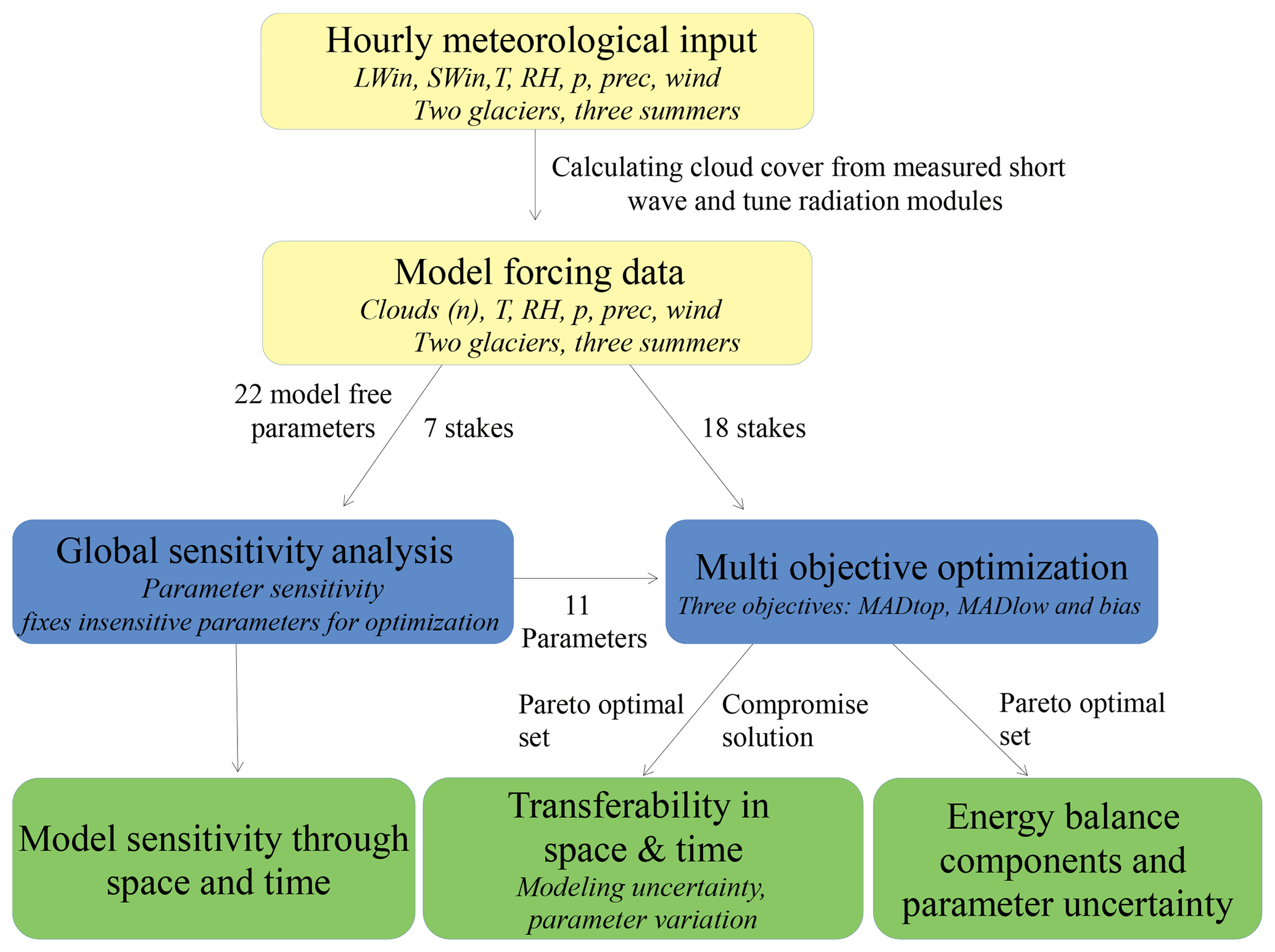
Figure 1The sequential approach used in this study can be classified in three steps. First, data management and model setup in beige, the simulations (blue) first use a global sensitivity analysis to reduce the parameter space followed by a multi-objective optimization. All simulations are performed independently for three summers on two glaciers. The data analysis (green) is done independently for sensitivity, parameter and model uncertainty analyses.
Mass balance models are required to be transferable in space and time in order to estimate run-off on a larger scale or the impact of a changing climate (Oerlemans et al., 2005; De Woul and Hock, 2005; Raper and Braithwaite, 2006). To study the transferability of an enhanced temperature-index model Carenzo et al. (2009) used the optimized parameters from one particular year and glacier and compared it to the locally optimized run at different glaciers and over different time periods. They concluded that their model shows a rather good transferability in space, except during overcast conditions. Furthermore, they observed that the parameters vary depending on year and location and are correlated to each other. MacDougall and Flowers (2011) and Prinz et al. (2016) investigate transferability of full energy balance models; while MacDougall and Flowers (2011) find satisfactory temporal transferability in the Arctic over 2 years, albeit with some local parameter adjustment, Prinz et al. (2016) fail to do so in the tropics over an interval of a century. This is attributed to a substantially changed climate over the century and/or different micro-meteorological setting due to dramatic glacier shrinkage (Prinz et al., 2016), which implies the problem of transferring a calibrated model to rather different climatic settings and glaciers and raises the question about the general uncertainty and transferability of such models.
It can be expected that models with more parameters have greater variation in their solutions. Reduction of free parameters for optimization based on a sensitivity analysis is therefore a helpful tool to reduce both the effect of parameter correlation and computational expense (Spear and Hornberger, 1980; Saltelli et al., 2000; van Griensven et al., 2006). Gurgiser et al. (2013) applied such a parameter reduction procedure on a tropical glacier to reduce the free parameters prior to assessing model transferability.
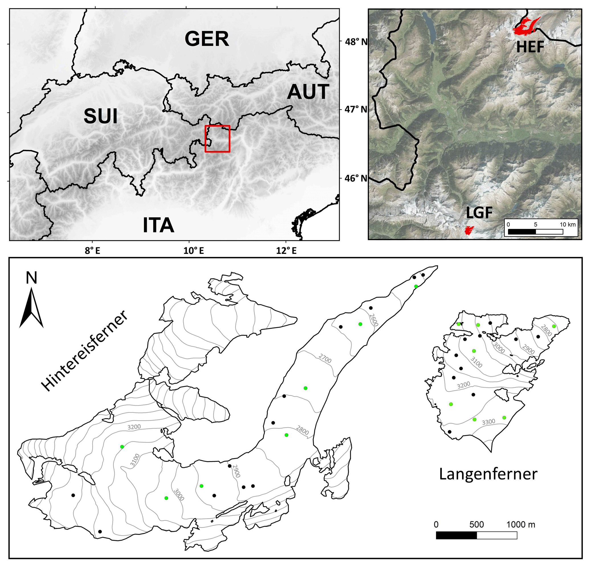
Figure 2Model simulations are performed at the stake locations shown as points; points marked in black are only used in the optimization, while green points indicate the seven stakes on each glacier that were also used in the sensitivity analysis. Detailed maps are available in the Supplement (Figs. S1–S2).
Model sensitivity and model uncertainty are often evaluated together, and assessments of varying robustness have been presented in the literature. For example, Mölg et al. (2012) used an arbitrarily chosen spread of the most positive and negative deviation simulations around their single best fit in respect to root mean square deviation (RMSD) of cumulative mass balance to estimate uncertainty. This gives only a rough estimate, as only two particular runs determine the uncertainty estimate. Anslow et al. (2008) first optimize their model and then vary the optimized parameters within certain bounds (5 %) and perturb the meteorological input to quantify the impact on the mass balance. This provides the sensitivity of the model output towards the parameter values and inputs, but the created range is also used as model error estimate. Machguth et al. (2008) perform a similar assessment but base their perturbation ranges on probability density functions, whereby model uncertainty is assessed by applying random and systematic errors and uncertainties to the meteorological input data as well as to the mean value of parameters. The reported uncertainty, of 700 kg m−2 for a 400-day simulation at a single point (roughly 10 % of the total melt), is related to the standard deviation of the probability density function. Rye et al. (2012) used multi-objective optimization to better constrain their model parameters but do not evaluate their model on independent observations (i.e. observations not used for calibration).
In this study, we present a model calibration and uncertainty assessment workflow built upon a combination of these ideas. Our aim is to bring awareness that uncertainty estimates of physically-based models with many free parameters are likely to be under-estimated when applied in different settings (geographical and or temporal) than those for which the model was calibrated. Using an established distributed energy and mass balance model (Mölg and Hardy, 2004; Mölg et al., 2008, 2009), we simulate 3 years of summer mass balances on two mid-latitude glaciers (Fig. 1). We start by applying a global sensitivity analysis to reduce the parameter space extending the local sensitivity analysis used by Gurgiser et al. (2013) to a global variance-based method (Saltelli et al., 2006), a procedure which has recently been applied in snow pack modelling (Sauter and Obleitner, 2015). Subsequently, we use the multi-objective optimization applied by Rye et al. (2012) to calibrate our model based on a set of three quality measures. The parameter uncertainty and resulting uncertainty of the energy components are evaluated based on this calibration procedure. Finally, the temporal and spatial transfer of such a model ensemble is assessed with cross-validation.
In this paper, we will use the term “model uncertainty” to describe the difference between any modelled quantity and its counterpart in reality (“the truth”). An uncertainty value is a measure of how much trust can be given to a modelled quantity: in practice, model uncertainty can be estimated based on observations, and in any modelling activity which includes parameter calibration model uncertainty must be estimated separately from the calibration procedure (cross-validation). For quantities without equivalent in reality (e.g. model parameters), we use the term “uncertainty” to refer to the fact that their true value is really unknown, and that this uncertainty in the parameters is also conveyed in the model uncertainty. When we speak from “model sensitivity”, we mean the variance of the model output as function of the variance of an input quantity (e.g. forcing data, model parameters). A model sensitivity analysis does not require observations. In our paper, we restrict our sensitivity analysis to the internal model parameters, not to the input meteorological variables.
Two glaciers in the eastern European Alps were selected as test sites in this study (Fig. 2). Hintereisferner (HEF; 46.80∘ N, 10.75∘ E) is a sizeable valley glacier in the Austrian Ötztal Alps that spanned 2454 to 3720 m a.s.l. in 2013, when the glacier area was ca. 6.7 km2. Langenferner (Vedretta Lunga) (LGF; 46.46∘ N, 10.61∘ E) is a smaller valley glacier in the Italian Ortler Alps that spanned 3370 to 2711 m a.s.l. in 2013. These glaciers were chosen since the model used here requires topographic and meteorological input data, and measurements of surface mass balance for evaluation. For both these glaciers (i) topographic data are available in the form of high-resolution digital elevation models (DEMs) derived from airborne laser-scanning data acquired in autumn 2013 (Galos et al., 2015); (ii) meteorological data are available from automatic weather stations (AWSs) in the vicinity of the glaciers for the period 2012 to 2014 and (iii) intense glaciological observations, including measurements of seasonal mass balance (e.g. Klug et al., 2017; Galos et al., 2017), are available.
At HEF the AWS is located on a small plateau within a rock slope north of the upper tongue area of the glacier at an altitude of 3025 m a.s.l. The horizontal distance of this AWS from the glacier is about 300 m and it provides all meteorological data required for the model except for precipitation. Precipitation data were taken from the gauge operated by the Bavarian Academy of Sciences at Vernagtbrücke, 3.5 km east of HEF at an elevation of 2600 m a.s.l., and were scaled to the elevation of the AWS on the basis of precipitation gradients derived from 11 totalizing rain gauges in the vicinity of the glacier (Strasser et al., 2017). At LGF the AWS data came from the station of the Hydrological Service of the province of Bozen operated at Sulden Madritsch, 2.5 km north of the glacier at an altitude of 2825 m a.s.l. (Galos et al., 2017).
3.1 Energy balance model
The energy and mass balance model used in this study is a process-based model that has been applied in a range of glacier environments (Mölg and Hardy, 2004; Mölg et al., 2008, 2009, 2012; Gurgiser et al., 2013; Prinz et al., 2016; Galos et al., 2017). The model was run in hourly time-steps for three summer periods over each glacier. The model is a distributed mass and energy balance model, but in this study simulations were limited to 18 stake locations on each glacier to reduce computational expense. The model tracks the accumulation of solid precipitation and uses the surface energy balance to calculate the ablation at the glacier surface:
where LWnet and SWnet are the net radiation balances for long-wave (thermal) and short-wave (solar) radiation and the other energy fluxes are the sensible (QS), latent (QL), ground (QG) and precipitation (QP) heat flux. The available energy is used to raise the glacier surface temperature (Qice) if below freezing point or for melting (QM) if the glacier surface is at the melting point. Mass losses of the glacier are represented via melt (QM) and sublimation (QL). Refreezing of liquid precipitation and resublimation lead to additional mass accumulation at the surface. We use the model in a similar configuration to Prinz et al. (2016). The only difference is given by a change in the short-wave radiation scheme which is explained in the detailed model description in the Appendix (Sects. A1–A6).
3.2 Methods
3.2.1 Global sensitivity analysis (GSA)
Variance-based sensitivity testing methods work in a probabilistic framework judging sensitivity by relative variances of model input and output (van Griensven et al., 2006; Saltelli et al., 2000, 2006, 2010). This is a global method that is independent of model calibration, i.e. independent of a local optimal run, and is hereafter referred to as global sensitivity analysis (GSA). The method treats the model as a simple function f with
where y is the single model result (in this case mass balance) and are the individual input parameters.
The influence of an individual parameter can be examined by the main effect (Vi) of Xi on Y.
X−i is the whole parameter space except any variation in Xi (a fixed Xi), E is the expectation value and V the variance. ) is the mean model output with whole parameter variation except in Xi. The variance over all values for Xi yield the variance attributed to parameter Xi. The sensitivity of the model towards single parameters is evaluated by normalizing by the total variance of the output.
is the first-order sensitivity index. The total sensitivity index () is the effect of Xi with all its interactions on the model variance:
This can be related to the sensitivity obtained from local sensitivity analysis. The model sensitivity (variance) to Xi is tested ()) at every point of the parameter space (X−i fixed). To clarify, consider the example of a simple non-additive model with the variables Xi as input parameters with a given variance/uncertainty. Assuming unified distribution within the intervals
leads to a model output range of . The variance-based method yields the results for , the first-order sensitivity index and , the total sensitivity index for an ensemble of 10 000 runs as shown in Table 1. The first-order effect of X3 is the largest, while the other two are similar if computational uncertainty is neglected. The most variance is caused by the last parameter. X3 has no interactions, so its total index is the same as the first-order one, while interaction between X1 and X2 creates additional variance, so their total index is higher. In the example X1 and X2 contribute to ≈60 % of the total variance and X3≈40 %, as and .
Table 1The sensitivity indices for the simple model . The indices for X1 and X2 are similar as they both have the same normalized variance. X1⋅X2 creates additional variance by the interaction of the two parameters yielding higher total indices.
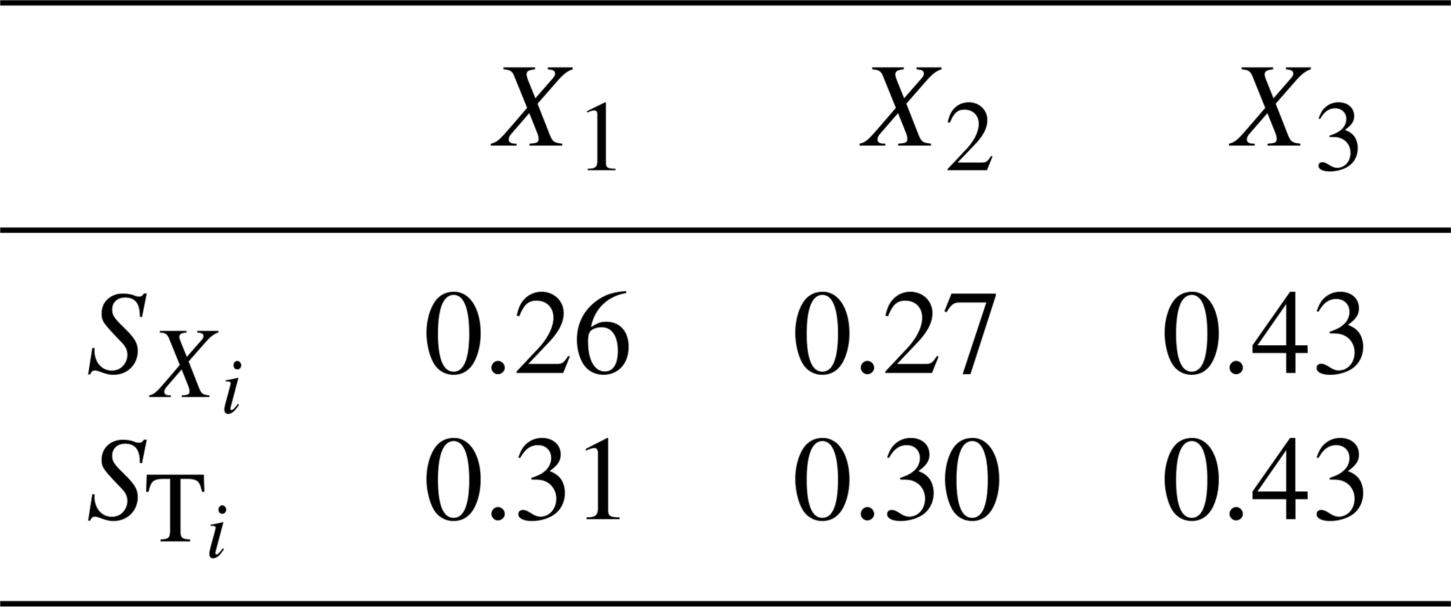
Table 2The ranges for the 22 different parameters used in the sensitivity study. Most parameterizations are explained in the Appendix A.
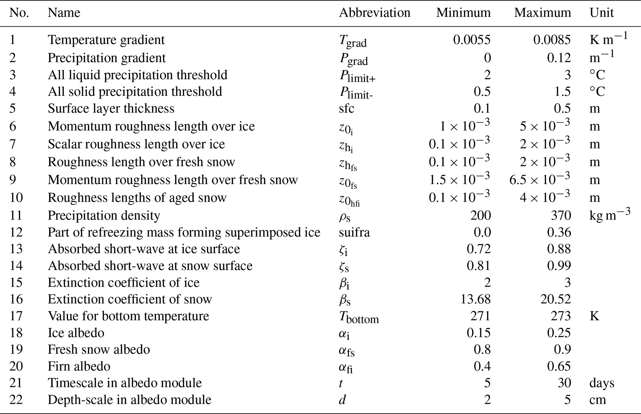
The estimation of the sensitivity indices follows the algorithm from Saltelli et al. (2010). The model used here has 22 free parameters. A base sample of 12 000 parameter settings was created with a quasi-random Sobol sequence. The random numbers are linearly transformed onto the parameter intervals. The distribution is always treated as uniform and the limits for every parameter are given in Table 2. The indices are estimated with runs, where k is the number of parameters and N the base sample size. The GSA consists of a total ensemble size of 300 000 simulations per year and glacier, fulfilling the convergence criteria for the algorithm (, , ). Note that we did not investigate if fewer solutions could already fulfill the convergence criteria. To reduce computational expenses the GSA model was limited to seven stake locations on each glacier (Fig. 2).
The parameter sensitivity results from the GSA are also used as a tool to reduce the number of free parameters in the model by identifying those parameters which have only a marginal influence on the model output (Spear and Hornberger, 1980; Saltelli et al., 2000; van Griensven et al., 2006). The model is considered insensitive to parameters with a total sensitivity index () of <0.05, and these parameters were fixed at the median value of the range shown in Table 2 in subsequent model simulations.
3.2.2 Multi-objective optimization and uncertainty quantification
A multi-objective optimization allows for more than one optimal solution in the calibration procedure, and offers a way to assess a range of plausible parameter sets that we will use later on for model predictions. The multi-objective optimization used here follows previous approaches in hydrology and glaciology (Yapo et al., 1998; Rye et al., 2012). Where the model is given n objectives, with fn to be minimized in respect to the model parameter input X, the optimization approach can be written as follows:
The result of Eq. (6) is an ensemble of optimal solutions that represent trade-offs between the objectives and no single one can be deemed superior to the other optimal solutions. Therefore, they are called the non-dominated set of optimal solutions, or Pareto set (Pareto, 1971). As an illustration, consider an optimization with two objectives (f1,f2): The concept of a Pareto optimal set is shown in Fig. 3 in which the (classic) single objective solutions are the points and for the two objectives. A solution at the utopian point is desirable as all functions would be at their minimum, but the models generally cannot optimize the different objectives simultaneously. There are only compromise solutions between the objectives. The members of the set of optimal solutions defining the Pareto front are superior to the other solutions, but are all equal to each other without subjective ranking by the modeler. The variation of the parameters of the optimal solution set defines the minimum parameter uncertainty (Vrugt et al., 2007). This uncertainty is a result of shortcomings in the model and/or the variations of parameters, such as spatial or temporal change in the true parameter value over the simulation period (Oerlemans and Greuell, 1986; Marshall and Warren, 1987). If a single simulation must be chosen to be the optimal model set up, the compromise solution, defined as the point with the lowest Euclidean distance to the utopian point, is a common choice.
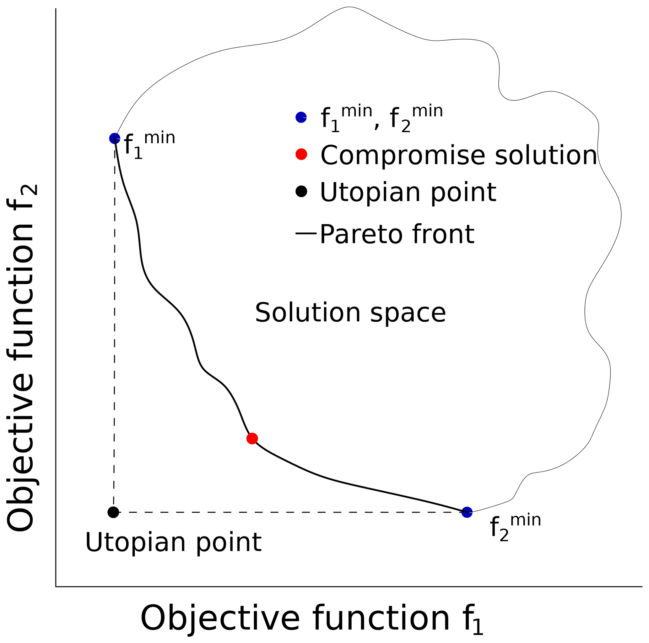
Figure 3The figure displays a 2-dimensional Pareto space which comprises a 2-dimensional Pareto front. The solutions on this front (black solid line) are referred to as the non-dominated set of solutions. In comparison, all other solutions within the solution space are inferior in at least one objective relative to the Pareto front. Classic single objective optimization yields the points and , which represent the minimum of those objectives that the model can achieve. The utopian point (black) is the point () where both objectives are at their minimal value. Commonly, the compromise solution (red) of the Pareto set is considered an objective choice for a single solution as it has the minimum Euclidean distance of the optimal solution towards the utopian point.
In this study the multi-objective optimization is based on a Monte Carlo simulation. The non-sensitive parameters from the GSA were fixed to their median value from the range used in the GSA (Table 2). Then 20 000 model simulations with random value combinations of the remaining parameters were created and the mass and energy balance were simulated for 18 stake locations. This approach was chosen in favour of an evolutionary algorithm so that different objective function spaces and all single objectives could be investigated with the same set of simulations. Various objective functions were initially explored, including root mean square deviation (RMSD) and mean absolute deviation (MAD) over all simulation points, but finally three objective functions that captured the main patterns of behaviour were applied: (i) the BIAS over all simulated stakes, (ii) the mean absolute deviation (MAD) of the lower nine stakes (MADlow9) and (iii) the MAD over the upper nine stakes (MADtop9). The BIAS is used as a proxy for the cumulative mass balance with the avoidance of interpolation errors. The RMSD is a commonly used measure for optimization in glaciological modelling (e.g. Gurgiser et al., 2013; MacDougall and Flowers, 2011). By using the MAD here we want to reduce the effect of individual stakes which could be influenced by processes which are not captured by the model (snow redistribution through wind or avalanches, dust and debris cover and related changes in radiation, etc.), but the general features of those two statistical functions are similar. Previous studies (e.g. Klok and Oerlemans, 2004; Hock, 2005; Sauter and Obleitner, 2015) have focused on the accumulation and ablation area separately or exclusively, but without a distinct mathematical comparison. Therefore, the approach of the split MAD was chosen. The Pareto front was identified, and a second ensemble including solutions within a certain range (100 kg m−2) from the Pareto front was additionally identified to account for errors in the field measurements of mass balance at each simulation point. However, results of this second ensemble will only be mentioned briefly throughout the discussion. The spread of the parameter settings of all optimal solutions of the Pareto and near-Pareto Sets are used to indicate the parameter uncertainty for each case, and the calculated surface energy balance components of these optimal sets are also used to estimate the uncertainty of the energy components on the point scale, as well as on the glacier scale.
4.1 Global sensitivity analysis
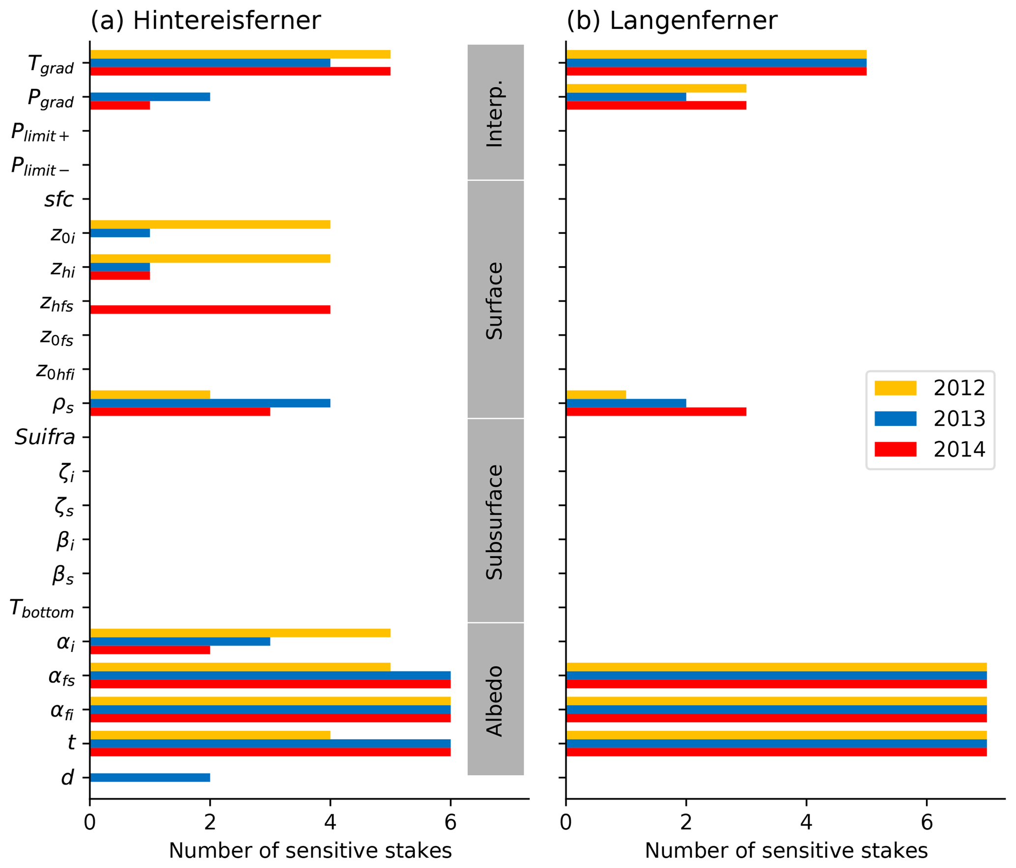
Figure 4The amount of sensitive stakes per year for (a) HEF and (b) LGF. The sensitivity analysis was performed at seven stakes on each glacier, though the vertical gradients can only be tested at six stakes as one is located at the same altitude as the reference weather station. Every parameter with a sensitivity index higher than 0.05 got a score of 1, giving a maximum count of seven per year (meaning the model is sensitive to this parameter at all stakes). Parameters involved in the parameterization of surface albedo are dominating, with snow related parameters in the upper section of the glacier and ice related ones at the lower stakes. Hintereisferner shows a total of 11 sensitive parameters and Langenferner 6.
The focus of this GSA is not on the absolute sensitivity towards single parameters, but rather to reduce the dimension of the parameter space. Therefore, the following discussion is limited to two classes: parameters to which the model is sensitive () and non-sensitive (). On each glacier the mass and energy balance at seven stake locations over 3 years was simulated for the GSA, so the maximum count of sensitivity for a parameter would be 21, meaning that the model is always sensitive to that parameter at every point of the glacier.
At Hintereisferner, 11 out of 22 parameters are identified as sensitive (Fig. 4a), and these sensitive parameters are classified in two general categories. Firstly, all but the lowest stake location are sensitive to parameters related to surface albedo, particularly of snow and firn, and secondly, for stakes with high elevation differences compared to the AWS, the model is also sensitive to the vertical temperature gradient.
The sensitivities show spatial and temporal variability, which can be explained by the varying mass balance conditions of the respective year (mean specific summer/annual mass balance with 2012: −2643/−1560, 2013: −1841/−510 and 2014: −1494/−122 kg m−2). For example, sensitivity to the ice-related parameters is most evident in 2012, which was the driest (in terms of precipitation, not air humidity) and most negative mass balance year, with large parts of the glacier surface free of snow and firn for most of the ablation season. By contrast, the roughness length of fresh snow is only influential at the upper stakes in 2014, where snowfall was frequent during the ablation season resulting in the least negative mass balance of the three study years. Sensitivity towards the elevational precipitation gradient is only relevant at the lowest stakes (500 m below the weather station) in the wet years.
On the smaller Langenferner, 6 of the 22 parameters were identified as sensitive (Fig. 4b). Similar to HEF, the model shows consistent sensitivity to surface albedo and the vertical temperature gradient. As LGF is smaller than HEF, the sensitivity shows less variability in space and time, though the annual mass balances during the three study years range from about −1500 to +400 kg m−2, and, as the tongue of LGF does not extend to such a low elevation as the one of HEF, it is less sensitive to ice-related parameters. Variations in the ice albedo within the bounds of 0.15 and 0.25 hardly influence the mass balance model results on the smaller glacier, even though ice is exposed for the majority of the summer at the lowest stake. This low sensitivity to the ice albedo compared to the snow albedo parameters is explained by the fact that, as the removal of snow cover is accompanied by a large drop in albedo (0.4–0.65 to 0.15–0.25), the time of exposure is more crucial than the final ice albedo, and this time of ice exposure is itself influenced by the snow albedo via its dominant control on the short-wave radiation budget. Within the chosen parameter ranges, the net short-wave radiation varies by 50 % in the case of fresh snow (10 %–20 % absorbed) and only by 12 % over ice.
4.2 Calibration
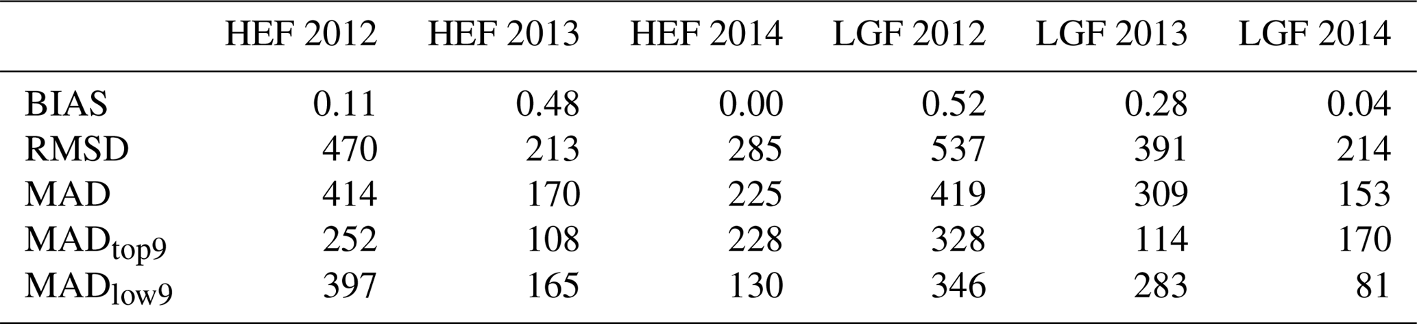
Table 3Five objective functions are used to analyse the model performance. The minimum value for every function and each year are given in kg m−2. While the BIAS is low in all cases, absolute errors and RMSD are much higher, and highest in 2012. Note that the minimum MAD does not refer to the same run over the whole glacier and its upper and lower parts.
First we consider the best model performance with respect to each individual objective function tested (Table 3), before presenting the multi-objective optimization based on the first, fourth and fifth objective in Fig. 5.
In all cases a model simulation with very low bias (<1 kg m−2) with respect to the stake mass balance can be found. This illustrates that apparently a good optimization on the single value of cumulative mass balance over the stakes is relatively easy to achieve (Table 3). In comparison, the deviation of all other objective functions is much higher, ranging from 81 to 537 kg m−2. The deviations in these objectives are all largest in 2012 on both glaciers. RMSD and MAD vary in a similar way between the years at each glacier, with the higher RMSD values indicating a non-uniform deviation from the measurements over the stakes. With the exception of 2014, the glacier-averaged MAD is larger than the MAD calculated for either the upper or lower section of the glaciers. This is to be expected as the stakes within each section of the glacier experience more similar climate conditions, resulting in a lower MAD. The fact that MAD in the lower glacier section is larger than in the upper section in 2012 and 2013 is probably related to the incapability of the model in its current configuration to correctly reproduce the date of ice exposure. In 2014 the upper glacier sections show a slightly higher MAD, associated with above average accumulation in the previous winter and the frequent summer snowfall in this season.
The multi-objective optimization, using BIAS, MADtop9 and MADlow9, yields an ensemble of solutions. The non-dominated set for each of the 3 years has 27, 17, 69 members for HEF and 58, 61, 14 members for LGF, respectively (Fig. S4). The fewest solutions are found in years with the lowest total MAD (HEF, 2013; LGF, 2014). Figure 5 shows the Pareto front of optimal solutions for HEF 2012 and the corresponding parameter settings. A low bias is easily achieved by the model if no other objectives are considered because it is a single value (the sum of the mass balance at all stakes) and, for example, deviations in the ablation and accumulation area may compensate each other. The projections onto the BIAS planes are less curved (the distance between the utopian and compromise point is smaller) and the performance in respect to the MADs can be drastically increased with only a small cost in the BIAS. The 2-dimensional projections of the Pareto space (Fig. 5a and b) illustrates, for example, that allowing for a model bias of 25 kg m−2 can improve the MAD by 200 and 300 kg m−2 in the lower and upper glacier sections, respectively. The MADs plane (Fig. 5c) is more curved (larger distance between the utopian and compromise point), indicating that the two objectives cannot be optimized by the model at the same time, such that some parameter sets leading to good results for the ablation zone of the glacier may not sufficiently reproduce the relevant processes in the accumulation zone.
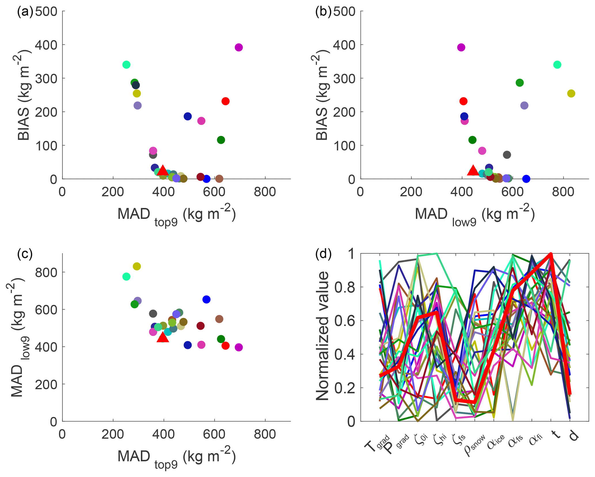
Figure 5Each individual member of the Pareto set for HEF in 2012 is displayed with a different colour and the compromise solution highlighted (red triangle or red line). The different panels are the 2-dimensional projections of the Pareto space onto the (a) BIAS and MADtop9; (b) BIAS and MADlow9; and (c) MADlow9 and MADtop9 planes. Panel (d) shows the normalized parameter values for each case in the same colours as in the Pareto space plots. The parameter settings of the optimal solutions are quite diverse and span over most of the parameter space. The firn albedo and albedo timescale are the only parameters showing some confinement to a narrower range. The chaotic nature of the parameter settings furthermore shows that a single solution is not representative in its parameter settings for the ensemble of optimal solutions.
The parameter values of those optimal solutions span the entire allowed space apart for some of those relating to snow albedo which span (almost) the whole parameter space in all years for both glaciers, and show no obvious tendencies towards a certain albedo range (Sect. 3). For HEF in 2012, snow albedo values cluster in the higher range (0.52–0.6) for firn and (0.86–0.9) for fresh snow (Fig. 5d), while on LGF lower firn and fresh snow albedo values (<0.5/<0.84) are optimal. Similar behaviour is observed for the albedo time scale (see Appendix A3), which tends towards higher values for HEF in 2012/13 and towards lower ones for LGF in 2013/14. The confinement of snow albedo is mainly a result of the highest model sensitivity towards this parameter, nevertheless it still varies and the converse argument, of less sensitive parameters showing greater span is not valid: for example, the roughness length over fresh snow is generally at the lower margin of the allowed parameter range (0.1– m) in 2012, even though the model is considered insensitive () to this parameter in that particular year. These results highlight that the parameter settings of multiple optimal solutions for this type of mass and energy balance models can vary drastically. There are no clear correlations between two individual parameters, instead all parameters interact simultaneously to some degree. Without the a priori reduction of model parameters by GSA, even less information could be extracted from the optimization. Compared to Rye et al. (2012) our parameters span a wider range of the normalized parameter space, which is due to a wider initial parameter range in our study. Despite the relatively narrow ranges of values reported in the literature, our study clearly reveals that many of the parameters could take almost any value in the optimization process. Changes to the parameter ranges accounting for potentially unrealistic values may quantitatively change the results, but within the range no change in the sensitive parameters is expected. For example, Rye et al. (2012) applied values for fresh snow albedo in the range of 0.65 to 0.95, while we restricted the initial range to values between 0.8 and 0.9, as reported in the literature (e.g. Cuffey and Paterson, 2010). We also used fresh snow densities which are relatively low compared to those reported in recent studies Helfricht et al. (e.g. 2018). However, the used values are based on previous studies (e.g. Mölg et al., 2008; Gurgiser et al., 2013; Prinz et al., 2016) and the choice of those does not significantly influence the results.
4.3 Transferability studies
To investigate the transferability of the optimized mass balance model settings, all the optimal solutions of the Pareto set of one glacier summer mass balance case were applied to the five other summer and glacier cases. While each Pareto set was identified based on the multi-objective optimization, the transferability study uses only the Euclidean distance towards the utopian point as a quantification tool. The individual optimal parameter settings for HEF 2012 for example yield quite varying performances for the other summers (Fig. S4a). While the performance on the same glacier (HEF) is reasonably good for 2012 (200–800 kg m−2 compared to 152–600 kg m−2 in the optimization period of summer 2013) and slightly worse for 2014, the optimal solutions do not perform so well for LGF, resulting in Euclidean distances of up to 3500 kg m−2. Analogous analysis of the ensemble behaviour of other summers shows that the optimal solution for 2012 also performs well in 2013 and vice-versa, and shows acceptable performance in 2014. The deviation of the 2012 and 2013 optimal values of HEF yields errors greater than 2000 kg m−2 on LGF. The 2014 HEF ensemble performs on average better on HEF, but two simulations perform better on LGF in 2012/13 and around 20 are within the same error as for HEF. On LGF also 2012 and 2013 agree better, and the ensembles produce reasonable results for both glaciers in 2014. The ensemble of 2014 on LGF yields similar errors (250–800 kg m−2) for LGF 12/13 and HEF 14. All ensembles of LGF produce larger errors on HEF in 2012 and 2013.
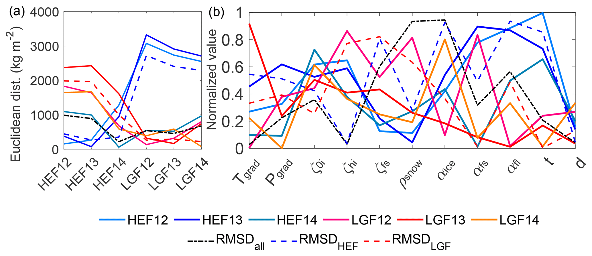
Figure 6(a) Performance of the single compromise solution for each season and glacier (GGGyy), with HEF in solid blue colours and LGF in red. The simulations which perform best over a 3-year (RMSDHEF and RMSDLGF) and 6-year period (RMSDall) are given with dashed lines, following the same colour scheme. (b) The corresponding parameter setting of the optimal solutions to the left. The colour scheme is equivalent. The compromise solutions for the individual years show different parameter settings and also varying performance out of the calibration period. Only the snow-albedo related parameters show a trend as they take rather large values on HEF and small on LGF. No clear trend is visible for the other parameters.
The cross-validation (Fig. 6) focuses on the transferability of the single compromise solution to other season and glacier cases. This can be considered as a classical best guess solution. The features follow the structure of the ensemble behaviour discussed above with HEF 2012 and 2013 seeming to be distinct from the other four cases. The compromise solutions for HEF 2012 and 2013 are similar in performance and parameter value and, while they perform adequately for HEF in 2014, within the estimated model uncertainty of 1300 kg m−2, the error is greater than 1500 kg m−2 when either of these compromise solutions is applied on LGF, no matter for which year. Similarly, the compromise solution for the 3-year period for HEF (RMSDHEF in Fig. 6), which is dominated by the characteristics of 2012 and 2013, also performs poorly when applied to LGF (errors of up to 3500 kg m−2). The compromise solution of HEF 2014, however, generally performs better on LGF than for other years at HEF, and reciprocally, the compromise solution over the whole period at LGF performs best at HEF in 2014, and the maximum error (up to 2500 kg m−2) is lower than for cases of HEF compromise solutions being applied to LGF. This is probably due to the domination of more negative mass balances in 2012 and 2013 at HEF, where good model performance is linked to capturing the large extent of the ablation area, whereas the shorter glacier tongue at LGF has smaller impact on the mass balance of this glacier. The compromise solution (RMSDall) for all six cases also highlights that within this set of six the cases HEF 2012 and HEF 2013 are more distinct from the other cases as the overall compromise solution performs worst in these two cases. For most parameters no clear separation between the two glaciers is evident, except for fresh snow albedo and the albedo timescale which are both larger at HEF and smaller at LGF. Inspection of the optimal parameter values reveals that runs with a longer calibration period (RMSDxxx) do not necessarily take trade-off values between the individual years. For example, in this case the solution that performs best over both glaciers and the whole time period (RMSDall) takes larger values of fresh snow density and ice-albedo than any other compromise solution (Fig. 6b). This further highlights the model complexity and is suggestive of the effects of physical shortcomings (such as parameter values that are constant in space and time) compensating each other.
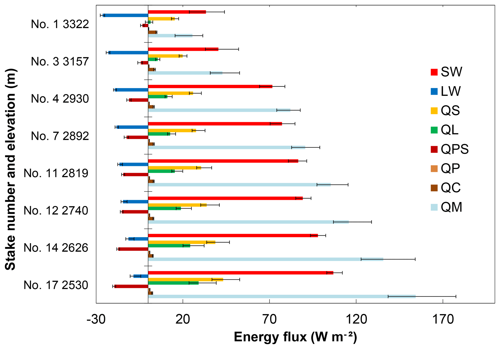
Figure 7The energy balance components for 8 out of 18 selected stake locations close to the central flow line, displayed in different colours for HEF 2012. Solid bars represent the fluxes of short-wave radiation (SW), long-wave radiation (LW), turbulent heat fluxes (QL and QS), penetrating short-wave (QPS), precipitation heat flux (QP),conductive heat flux (QC) and the resultant available heat for melting (QM, here plotted as a positive flux).
4.4 Energy balance components
Analysis of the energy balance components associated with Pareto set solutions offers a qualitative means of verifying that the identified optimal parameter settings are in line with expected physical processes at the glacier surface. The energy balance components calculated by the model are expected to vary depending on the parameter settings of an optimal ensemble, which have been demonstrated to span almost the whole parameter space. This variation in energy balance components is indicative of the uncertainty in the modelled energy fluxes (we say “indicative”, because the true uncertainty can only be assessed using observations, which are not available here). Figure 7 illustrates such variations in the energy balance components for the case of HEF 2012 based on the our model, not accounting for uncertainties in the meteorological input itself. In this case, the most uncertain energy balance component is the short-wave radiation, which at the same time is the largest energy source for the surface. Total energy flux from short-wave radiation decreases with altitude, while the associated uncertainty increases. The sensible and latent heat flux provide a net energy source to the surface and their value and uncertainty also decrease with altitude. The long-wave radiation budget is a net energy loss from the surface in summer, and its value increases and uncertainty decreases with elevation. As a result of these elevational patterns in uncertainty, the uncertainty in melt energy is also largest at low elevations.
The variation of the averaged energy components over the stakes for HEF 2012 are given in Fig. 8. The uncertainties are generally lower than on a stake basis. The short-wave, conductive ground heat flux and sensible heat flux supply a net heating to the surface on both glaciers. The precipitation heat flux is also a minor energy source. The penetration of short-wave radiation and the long-wave budget remove energy from the glacier surface. Latent heat is the only energy flux that has either a positive or negative effect on the surface energy balance depending on stake location, glacier and year. On both glaciers, lower elevation locations tend to show more positive energy fluxes from latent heat. At HEF this flux is mostly an energy addition to the glacier surface while on LGF it mostly serves to remove energy from the surface. In the beginning of the summer, sublimation during the day and condensation or re-sublimation during the night is dominant on HEF, and the general trend over the summer is to progressively more condensation. LGF shows less condensation during mid-summer, which is mainly attributed to less windy conditions than at HEF.
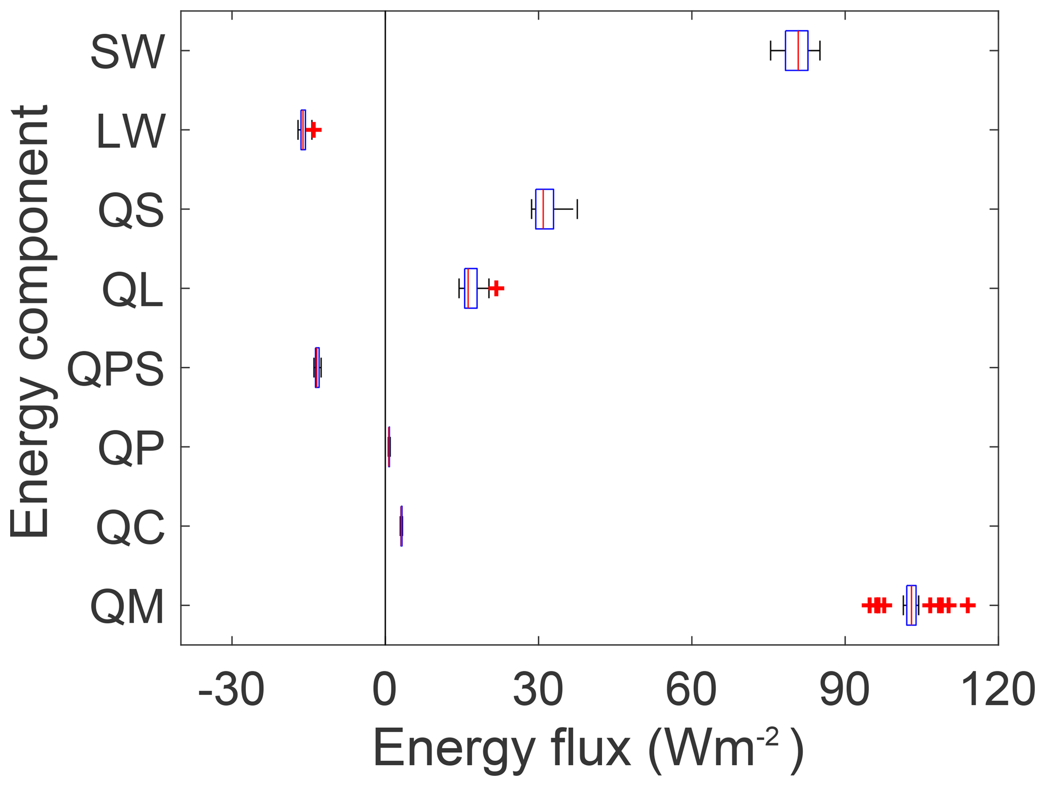
Figure 8The energy balance components averaged over all stakes has less uncertainty than on the point scale for HEF 2012. The objective functions are all integrated over the whole glacier and thus the uncertainty is lower. Glacier wide the short-wave radiation is the largest component with the largest absolute uncertainty as well, followed by the turbulent fluxes. The long-wave balance and the penetrating short-wave radiation provide a net cooling effect for the surface.
Table 4The energy balance components are averaged over all stake locations. The uncertainty is given in respect to the minimum and maximum of the ensemble. The short-wave radiation (SWnet) has the largest impact, decreasing in importance from 2012 to 2014, with a less negative mass balance (QM). The penetrating short-wave radiation (QPS) follows the same pattern with the opposite effect. The long-wave budget (LWnet) is lower for LGF. The turbulent fluxes are greatest in 2012 and larger on HEF. The precipitation (QP) and convective (QC) heat flux are of minor importance.
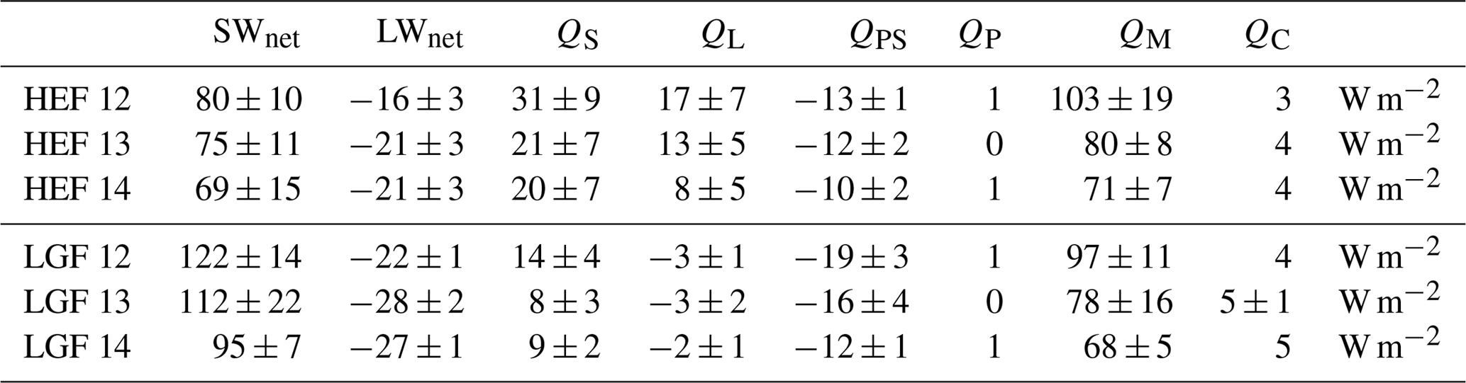
The total contribution of the energy balance components averaged over the glacier are listed in Table 4. The relative uncertainties of the energy balance components are up to 50 % of their contribution on single stake basis and 30 % averaged over HEF; slightly lower (30 % and 25 %, respectively) for LGF. This leads to a variation in the available heat for melting and the mass balance of about 30 % on a point scale. The absolute uncertainty of the seasonally averaged available energy for melting can reach up to 35 W m−2 at the tongue area of HEF. This corresponds to a daily melt uncertainty of 9 kg m−2 and seasonal uncertainty of up to 1.3 kg m−2. The glacier averaged available heat for melting is much less uncertain over all stakes. This is a result of the calibration process. The sum of total available melt energy is directly linked to the bias as objective function, which shows the largest value among the optimal solutions on HEF 2012 with 600 kg m−2. In comparison the MADs which are more influenced by the mass balance at the individual stake reach values up to 1000 kg m−2.
The largest uncertainties in our study are associated with the short-wave radiation as a result of the albedo parameterization, which relies on five model parameters. Alternative albedo parameterizations are also known to be a source of substantial uncertainty (e.g. Klok and Oerlemans, 2004; Willeit and Ganopolski, 2017). The greatest uncertainty is commonly found in the accumulation area and around the equilibrium line altitude. This is because (i) the parameterization for snow albedo has more variation and free model parameters than albedo over ice, and (ii) around the ELA the variation of the ice exposure date increases the uncertainty of short-wave radiation flux. Point scale albedo measurements combined with localized optimization schemes may solve this issue, but for distributed models a more detailed model may be necessary to better capture the full complexity of the processes governing initial snow albedo and its change through time (e.g. Flanner and Zender, 2006).
The long-wave radiation shows a lower uncertainty in this study than in Sauter and Obleitner (2015) and its uncertainty is mainly due to the air temperature, the related temperature gradient parameter, and the surface temperature. It is important to note that we cannot state that the general uncertainty of energy balance models associated with incoming long-wave radiation is low, since in this study the parameterization was optimized prior to the sensitivity analysis as direct measurements are available at the weather station. Consequently, long-wave radiation is considered a meteorological forcing here and therefore it was decided to do this prior optimization. The parameterization gives no bias for the station but the hourly RMSD was up to 30 W m−2, which is in the range of the net long-wave budget. This therefore also mainly influences short-term differences in the long-wave budget rather than the seasonal energy flux. Nevertheless, as with albedo, it remains unclear whether long-wave radiation modules based on air-temperature, cloudiness and sky-view factor are sufficient to model spatio-temporal variation over a glacier.
The turbulent fluxes are associated with the second largest uncertainty in this study, which is in agreement with other studies that found larger uncertainties in the radiative forcing (Willis et al., 2002). Turbulent fluxes are important for determining short-term variations of melt rates due to, for example, changes in the stability regimes (Lang, 1981). However, the uncertainties in our model are due to differences in roughness lengths and the temperature gradient. Roughness lengths over ice and snow vary substantially (e.g. Braithwaite, 1995) in space and time (Greuell and Konzelmann, 1994; Calanca, 2001). The appropriateness of using constants for these values in glacier modelling is also questionable, and stability corrections may differ from the glacier margins to the interior, for example. It is therefore also questionable how appropriate constant roughness lengths and stability corrections for ice and snow in space and time are. Furthermore, recent studies (Sauter and Galos, 2016) showed that the application of the bulk approach in complex mountain terrain can generally be problematic.
Heat supply from rain is negligible in our study, which is in agreement with other studies on alpine glaciers (e.g. Hock, 2005).
4.5 Implications of this study
The larger glacier, Hintereisferner, has more sensitive parameters and the variation over the stakes is larger than at Langenferner, as a result of more distinct climate regions on the longer tongue of the larger glacier. This is also true for the uncertainty of energy balance components, with the exception of the net solar radiation, which is comparable on both glaciers. Short-wave radiation is the most uncertain of the energy balance components, due to the albedo parameterization, which accounts for the change in albedo over time, but does not account for any possible spatial variation in temperature or grainsize-dependent albedo decay rates. We have shown that the model has difficulties optimizing the upper and lower part of the glacier simultaneously, as a result of the variable parameter values of physical quantities like albedo. The large spread of our ensemble is a result of trade-off solutions between the real albedo at any time and any location and the temporally and spatially averaged parameterization applied. Other parameterizations that are assumed as constant in space and/or time, or only indirectly affected by temperature and altitude dependencies, are also subject to similar trade-off effects. Although the physical relations may not be the same at all times and the lower tongue area may be quite different from the upper glacier, this does not mean that the model performance is worse on the larger glacier (HEF) with more variation in a quantitative matter (Table 3), but rather that the solutions of the Pareto front show more variation in the parameter settings. This analysis clearly identifies the issue of governing parameters and parameterizations not being constant in space and time as the main problem of distributed energy balance modelling. The most readily appreciable example in this regard is ice albedo, which is often lower near the terminus due to debris and dust accumulation and water saturation of the glacier surface.
To improve this we suggest two potential approaches: (1) although optimizing all key parameters serves a purpose for a broad range of applications, fixing low sensitivity parameters to common values, which are not optimized, results in a type of a simplification of the model that reduces over-fitting and potentially increases the stability and comparability of the energy balance model over short-timescales. The overall performance of such a model will be lower because the tuning possibilities have been restricted, but better estimates of the model uncertainties for out-of-sample periods can be generated. (2) Parameters or parameterizations could be allowed to vary in space and/or time. This could be achieved either by increasing the measurements and data availability or increasing the model complexity. More complex albedo schemes are available, for example, for snowpack models like Crocus (Vionnet et al., 2012) or SNOWPACK (Lehning et al., 2002). However, if new parameterizations are introduced they require sufficient field data to constrain the physical process and should not be just added as additional model free parameters to optimize.
The approaches in this study are helpful tools to combine these suggestions. A clear understanding of the model sensitivity, independent of the optimization of the model is necessary to decide on the importance of certain parameters. It gives the option of fixing parameters and focusing on the key processes. We have shown that multi-objective optimization is a valid tool to assess uncertainties in the model. The objectives used are all based on the same data (i.e. stake data). This allowed us to show the uncertainty that is just associated with treating the available data in a different way without requiring additional measurements. The model can readily be optimized to minimise bias or meet any single value objective; therefore, model performance based on single best-fit approaches should be treated with caution. Furthermore, a single solution may suffer significantly from parameter over-fitting and is not representative in its parameter settings for other plausible solutions. The chosen objectives show that there is inter-annual variation in the performances of the upper and lower section of the glacier in our cases. The curved nature of the Pareto front highlights that simultaneous optimization of both areas is difficult for the model. Parameters are just not constant in either space or time, so the model uncertainty increases when the model is applied to other time periods or on another glacier. The model uncertainty is in the range of 1000 kg m−2 per summer season for each glacier. It is larger when transferring the calibrated model to another alpine glacier, but still of the same order of magnitude. Our results reveal larger model uncertainties related to spatial transfer than found in previous studies (MacDougall and Flowers, 2011). This can be explained by the relatively large inter-annual variability of mass balance, as well as the comparably large distance between the glaciers in our study. Together with an uncertainty estimation of the energy balance components the key parameterizations, which need further improvement, can be identified. Furthermore, within the multi-objective framework it is possible to focus on processes individually: for example if the albedo is measured on the point scale, the difference to its model value could be used as an objective, instead of an a priori calibration of the albedo parameterization itself.
Neither meteorological forcing on the point scale nor mass balance measurements are free of errors, and the related model uncertainties were not formally disentangled from other uncertainties in this study. Zemp et al. (2013) have estimated an annual measurement uncertainty of 140 kg m−2 on point scale glaciological mass balance measurements, while Galos et al. (2017) report somewhat lower values for Langenferner. More information about the propagation of those errors is needed to quantitatively include them in the optimization. However, if an uncertainty of 50 kg m−2 in the MAD and BIAS is included, the Pareto sets increase by 1 order of magnitude. This complicates further interpretations and increases the total model uncertainty.
The analysis presented here indicates that while mass and energy balance models help us to understand the physical processes on the glacier, the necessity for parameterizations within these models introduces considerable, variable uncertainty to the model output. Calibration of surface mass balance models is complex and uncertainty studies are helpful to understand those models, and it is not advisable to draw general conclusions from such modelling efforts without first fully understanding the inherent model sensitivity and the properties of the uncertainty of the calculated mass balance and associated energy fluxes in detail.
Based on a well developed mass and energy balance model, applied to two well-studied glaciers in the European Alps, this study gives a robust estimate of the model uncertainty and discusses the advantages of parameter space reduction and multi-objective optimization in glaciological modelling.
Using a variance-based global sensitivity method, model sensitivity to the free model parameters was identified, independent of the calibration data. Model sensitivity to specific parameters is both site- and time- specific, and this should be acknowledged in wider applications of such models. By separating the parameters into two sensitivity categories, the model parameters to be optimized can be reduced. Those that the model output is sensitive to were subject to a multi-objective optimization, while non-sensitive parameters were fixed to literature values.
The multi-objective optimization was based on three objectives related to stake mass balance data measured using the glaciological method. We used the model bias over all stakes and the mean absolute deviation over the upper and lower part of the glaciers. It proved difficult to optimize model performance in the upper and lower section of the glacier simultaneously. The bias over all stakes, which was used as a proxy for the cumulative mass balance, can be minimized easily, and this should be considered when optimizing for a single best fit against single values. The ensemble of optimal solutions shows a wide spread of parameter settings within the physically reasonable range. This implies that the common approach of a single best optimized parameter set is subject to over-fitting and may significantly differ from other equally plausible solutions, meaning that they are not representative by default. Furthermore, our results show that the constraint of plausible parameters is only marginally linked to the sensitivity, with very sensitive parameters also taking multiple optimal values. This implies that keeping these parameters constant in space and time increases the model uncertainty. The overall model uncertainty (not accounting for uncertainties related to meteorological forcing data) is in the range of 1000 kg m−2 per summer season on the same glacier, and increases when applied to the other glacier. The model performance is worse when applied to another glacier, but is of the same order of magnitude as for the temporal transfer, suggesting the model can be applied, within its uncertainty, to other glaciers with similar climatic settings.
Parameter uncertainty is connected with uncertainty in the energy balance components, which, in the cases studied here, reached 30 % averaged over the glacier and 50 % at individual stake locations. In our study the most uncertain energy balance components are the net short-wave radiation and the turbulent fluxes, reasserting the findings of other studies (e.g. Van De Wal et al., 1992; Klok and Oerlemans, 2002) that indicate the snow and ice albedo representation is the most crucial parameter on mid-latitude glaciers for the summer mass balance.
Overall, the findings of this study highlight that understanding the sensitivity and uncertainty of surface energy and mass balance models is complex, and simplistic assessments, in particular single best guess approaches, of model performance are likely to overstate model capabilities. Further studies such as this, incorporating more models, glaciers and years would help to constrain the degree to which results from such models can be considered reliable for regional applications and for projections of glacier mass balance.
The code of the mass balance model can be requested from Thomas Mölg (thomas.moelg@fau.de). Pareto construction scripts and the updated solar module can be requested directly from Tobias Zolles (tobias.zolles@uib.no).
The mass balance and meteorological data used in this paper are available at Zenodo; https://doi.org/10.5281/zenodo.1326398 (Zolles, 2018). All mass balance data are publicly available through the WGMS (https://wgms.ch/products_ref_glaciers/hintereisferner-alps/, last access: 1 June 2018, Juen, 2018).
The mass and energy balance model used here consists of coupled surface and subsurface components. The model computes mass balance as the sum of solid precipitation, surface deposition, internal accumulation (refreezing of liquid water in snow), change in englacial liquid water storage, subsurface and surface melt and sublimation. This approach is based on the surface energy balance of a glacier in the following form:
where SWnet is net short-wave radiation, LWnet is the sum of incoming and outgoing long-wave radiation at the glacier surface; QS and QL are the turbulent fluxes of sensible and latent heat, respectively; QG is the subsurface energy flux comprised of QC; the conductive heat flux in the subsurface; and QPS is the energy flux from short-wave radiation penetrating into the subsurface, and finally, QP is the heat flux from precipitation. The sum of these fluxes yields a residual flux F which, if the glacier surface temperature (TS) reaches 273.15 K, represents the latent energy for melting. If TS is below 273.15 K, energy conservation is achieved by solving TS to balance the fluxes (e.q. Mölg et al., 2009). The model is fully described in the previously mentioned publications and briefly below.
A1 Long-wave radiation
The calculation of the incoming long-wave radiation is based on Stefan–Boltzmann law (Mölg et al., 2009; Klok and Oerlemans, 2002; Konzelmann et al., 1994):
with σ being the Stefan–Boltzmann constant and ϵ the emissivity:
where “cs” and “cl” are the clear-sky and cloud emissivity, respectively, n is the cloud cover fraction calculated in the solar module as neff and p is an exponent related to the importance of cloud emissivity (Greuell et al., 1997). The cloud emissivity is computed using
with ea as the atmospheric vapour pressure. The three parameters ϵcs, p and b were optimized (using a 5000 member Monte Carlo) to reproduce the measured long-wave radiation. First the runs within 10 % of the best run, in respect to a weighted average of BIAS and RMSD, between the simulated and the measured incoming long-wave radiation at the HEF Station were determined. The run of this ensemble with the lowest RMSD/BIAS on LGF was taken as the best compromise solution. The parameters are fixed within the model for the whole study period and are based on three summers of data at HEF and one and a half at LGF (therefore a larger impact of the longer data at HEF on the optimization). The trade-off values are taken to be applicable on both glaciers with the final values of b=0.515, n=1.95 and ϵcs=0.994. These setting results in an hourly RMSD below 31/37 W m−2 for HEF/LGF and no bias, not far from the optimal setting for either glacier with 30/36 W m−2.
The outgoing long-wave radiation follows the Stefan–Boltzmann law as in Eq. (A2), with T the glacier surface temperature and the emissivity of ice ϵi is assumed 1.
A2 Convective fluxes
The latent heat flux (QL) and the sensible (QS) are computed similar to Mölg and Hardy (2004). The calculations are based on the Monin–Obhukov similarity theory (Garratt, 1992).
with Lv being the enthalpy of vaporization (2.514 MJ kg−1), ρ0 the air density at mean sea level (1.29 kg m−3), p0 is 1013 hPa, κ the van Karman constant (0.4), ea is the water vapour pressure in air and Es the surface value, respectively. and z0ν are the momentum and scalar roughness length of water vapour. zm and zv is the height above ground where the wind speed and the water vapour (ea) is measured and calculated. The sensible heat flux
is computed with cp, the specific heat of air at constant pressure, Ta, Ts the air and surface temperature and zh the scalar roughness length for temperature. The roughness lengths (zj) are a model free parameters in this study. The model distinguishes three different roughness lengths depending on the glacier surface: fresh snow, firn and ice. For a stable stratified atmosphere, a stability correction based on Phi functions is applied (Mölg and Hardy, 2004).
A3 Surface albedo and the albedo module
The albedo parameterization is based on Oerlemans and Knapp (1998). It computes the broadband albedo for each grid cell, based on the ice and snow albedo and the depth of the snow pack:
αice is a model free parameter d is the snow depth, and d* is the characteristic scale for the snow depth and a free parameter (Oerlemans and Knapp, 1998). The relation for the snow albedo (αsnow) is
with αfirn, αfreshsnow and t* as model free parameters subject to optimization. The albedo module (t*) is a characteristic time scale in days (Klok and Oerlemans, 2002) and t the time since the last snowfall event (>0.1 cm fresh snow).
A4 Surface temperature and ground energy flux
The conductive heat flux (QC) and the energy flux from penetrating short-wave radiation (QPS) determine the ground heat flux (QG) of the energy balance (Eq. 1). The model solves the thermodynamic energy equation for a multi-layer grid with a fixed bottom temperature (15 Layers, 0.1 m steps in the first metre, gradually increasing to a total depth of 7 m). The bottom temperature is a model free parameter. QC is computed from the temperature difference between the surface and the first layer.
The calculation of the penetration of short-wave radiation is based on Bintanja and Van Den Broeke (1995). A constant fraction (1−ζi) of the net-short-wave radiation is penetrating the surface and the intensity is exponentially decreasing with depth. The optimization and sensitivity analysis in this study uses four parameters with the extinction coefficient and the absorbed fraction (ζi) for snow and ice.
A5 Surface accumulation and precipitation
The surface accumulation is directly related to the precipitation. The model has two threshold values for all liquid and all solid precipitation (Mölg et al., 2012). In between these thresholds, the portion increases linearly. The temperature threshold and the density of solid precipitation are subject of the sensitivity analysis and optimization.
A6 Solar module and solar module sensitivity
The parameterization of the short-wave radiation is based on the calculation of the cloudiness, in the form of the effective cloud cover fraction neff:
with SWmea being the measured short-wave and Dcs, Scs the calculated diffuse and direct radiation under clear sky conditions. The parameter k determines at which fraction of the clear sky value full cloudiness is achieved; i.e. all incoming radiation is diffuse. It is important to note, we allow neff>1 if such low radiation was measured. The influence of k on the model output was investigated (Appendix A6). The calculation of the clear sky values is described in Mölg et al. (2009). The diffusion portion of radiation under clear sky conditions was determined using a manual selection of clear sky days. The values varied between the snow free (Kdif=0.51) and snow covered days (Kdif>0.65). For the calculations an averaged value of 0.6 was used. As Kdif is a fixed glacier wide value, while snow cover might vary, a modulation depending on the conditions at the weather station is not possible. The applicability of Kdif as a single value might need to be reevaluated for other models, applications and research questions.
The calculation of the incoming short-wave radiation on every point of the glacier is based on the assumption of homogeneous cloudiness (neff). It is a reversing of Eq. (A9)
with SWdiff being the calculated diffuse radiation and pdiff the portion of diffuse radiation under clear sky conditions. pdiff is calculated as the ratio of the clear sky diffuse and total radiation. It was 0.084 and 0.085 for the two glaciers and set to 8.5 % (for both to have a common value). Compared to previous works using the solar module, we changed the increase of diffuse radiation. Instead of a linear increase of diffuse radiation, the portion of diffuse radiation is linearly increasing with increased cloudiness. This is a basic parameterization and reproduces the measured radiation fully. Via neff, k is determining the ratio of direct and diffuse radiation. This could alter the energy balance. The direct radiation is calculated analogously and corrected for slope and aspect.
The calculation of solar radiation incorporates the free parameter k, which determines at which fraction of the total possible global radiation everything is considered as diffuse radiation. The parameter k varies with latitude (Hastenrath, 1984) and is not constant in time either; therefore the effective cloud cover incorporates some of its variability and is not exactly the cloudiness (Mölg et al., 2009). With the new parameterization (Eq. A10), the global solar radiation at the weather station can be fully reproduced so k cannot be optimized. But it determines the portions of direct and diffuse radiation, which may have a significant influence on the energy and mass balance. Therefore, an additional GSA was performed with the parameter k as the 24th model free parameter. Based on the values for the tropics 0.65 (Mölg et al., 2009) and the Arctic with ≈0.85 (Hock and Holmgren, 2005) it was varied in this range for the sensitivity analysis. Its maximum sensitivity index over all seven investigated stakes in the GSA was , which is 1 order of magnitude lower than the threshold for our sensitive parameters. Therefore, the choice of k within the given range is not influential on the simulation of the mass balance on the glacier. The model albedo does not vary between direct and diffuse radiation, so it only influences the total amount of radiation at less or more shaded areas than the weather station.
Furthermore, the change in the calculation of direct and diffuse components from linear with cloudiness to a linear increase of the fraction are better suited to represent the site radiation. This is in agreement with the measured radiation by Hock and Holmgren (2005) on the Arctic glacier, Storglaciären (Fig. S5). The slightly higher starting value (pdiff) is due to larger portion of diffuse radiation under clear sky conditions in the Arctic than in the mid-latitudes, and the higher final value is due to a smaller k in this study (0.8) compared to around 0.85 in the Arctic. The influence of this change in parameterization is probably also rather small, as the model is not sensitive to changes in the relative fractions of diffuse and direct radiation on the chosen glaciers and stake locations.
The supplement related to this article is available online at: https://doi.org/10.5194/tc-13-469-2019-supplement.
TZ conducted the simulations and the data analysis and wrote the main part of the manuscript. FM was involved in defining the study and contributed to the statistical analysis. WG was involved in the model set-up and the adaptation of the solar module. SG was responsible for the mass balance measurements and data acquisition. LN contributed to the paper design and writing. All authors contributed to finalizing the paper.
The authors declare that they have no conflict of interest.
The computational results presented have been achieved (in part) using the
HPC infrastructure LEO of the University of Innsbruck. We thank Rainer Prinz
for supplying the snow, density and DEM grids for the energy balance model.
We thank the Hydrographisches Amt Bozen and the Hydrographischer Dienst Tirol
for funding the mass balance measurements. Lindsey Nicholson was supported by
the Austrian Science Fund Grant number V309.
Edited by: Tobias Sauter
Reviewed by: Matthieu Lafaysse and
one anonymous referee
Anslow, F. S., Hostetler, S., Bidlake, W. R., and Clark, P. U.: Distributed energy balance modeling of South Cascade Glacier, Washington and assessment of model uncertainty, J. Geophys. Res.-Earth, 113, 1–18, https://doi.org/10.1029/2007JF000850, 2008. a
Beven, K.: Changing ideas in hydrology - The case of physically-based models, J. Hydrol., 105, 157–172, https://doi.org/10.1016/0022-1694(89)90101-7, 1989. a
Beven, K. and Binley, A.: The Future of Distributed Models: Model Calibration and Uncertainity Prediction, Hydrol. Process., 6, 279–298, https://doi.org/10.1002/hyp.3360060305, 1992. a
Bintanja, R. and Van Den Broeke, M.: The surface energy balance of antartic snow and blue ice, J. Appl. Meteorol., 34, 902–926, https://doi.org/10.1175/1520-0450(1995)034<0902:TSEBOA>2.0.CO;2, 1995. a, b
Braithwaite, R. J.: Aerodynatnic stability and turbulent sensible-heat flux over a melting ice surface, the Greenland ice sheet, J. Glaciol., 41, 562–571, https://doi.org/10.1017/S0022143000034882, 1995. a
Brock, B. W., Willis, I. C., and Sharp, M. J.: Measurement and parameterisation of albedo variations at Haut Glacier d ' Arolla , Switzerland, J. Glaciol., 46, 675–688, https://doi.org/10.3189/172756506781828746, 2000. a
Calanca, P.: A note on the roughness length for temperature over melting snow and ice, Q. J. Roy. Meteor. Soc., 127, 255–260, https://doi.org/10.1002/qj.49712757114, 2001. a
Carenzo, M., Pellicciotti, F., Rimkus, S., and Burlando, P.: Assessing the transferability and robustness of an enhanced temperature-index glacier-melt model, J. Glaciol., 55, 258–274, https://doi.org/10.3189/002214309788608804, 2009. a, b
Cuffey, K. M. and Paterson, W. S. B.: The physics of glaciers, Academic Press, 2010. a
De Woul, M. and Hock, R.: Static mass-balance sensitivity of Arctic glaciers and ice caps using a degree-day approach, Ann. Glaciol., 42, 217–224, https://doi.org/10.3189/172756405781813096, 2005. a
Flanner, M. G. and Zender, C. S.: Linking snowpack microphysics and albedo evolution, J. Geophys. Res.-Atmos., 111, 1–12, https://doi.org/10.1029/2005JD006834, 2006. a
Galos, S. P., Klug, C., Prinz, R., Rieg, L., Dinale, R., Sailer, R., and Kaser, G.: Recent glacier changes and related contribution potential to river discharge in the vinschgau / Val Venosta, Italian Alps, Geogr. Fis. Din. Quat., 38, 143–154, https://doi.org/10.4461/GFDQ.2015.38.13, 2015. a
Galos, S. P., Klug, C., Maussion, F., Covi, F., Nicholson, L., Rieg, L., Gurgiser, W., Mölg, T., and Kaser, G.: Reanalysis of a 10-year record (2004–2013) of seasonal mass balances at Langenferner/Vedretta Lunga, Ortler Alps, Italy, The Cryosphere, 11, 1417–1439, https://doi.org/10.5194/tc-11-1417-2017, 2017. a, b, c, d, e
Garratt, J.: The atmospheric boundary layer, in: Cambridge Atmospheric and space science series, Cambridge University Press, Cambridge, 336 pp., 1992. a
Greuell, W. and Konzelmann, T.: Numerical modelling of the energy balance and the englacial temperature of the Greenland Ice Sheet. Calculations for the ETH-Camp location (West Greenland, 1155 m a.s.l.), Global Planet. Change, 9, 91–114, https://doi.org/10.1016/0921-8181(94)90010-8, 1994. a, b
Greuell, W., Knap, W. H., and Smeets, P. C.: Elevational changes in meteorological variables along a midlatitude glacier during summer, J. Geophys. Res., 102, 25941, https://doi.org/10.1029/97JD02083, 1997. a
Gurgiser, W., Marzeion, B., Nicholson, L., Ortner, M., and Kaser, G.: Modeling energy and mass balance of Shallap Glacier, Peru, The Cryosphere, 7, 1787–1802, https://doi.org/10.5194/tc-7-1787-2013, 2013. a, b, c, d, e, f, g
Hastenrath, S.: The glaciers of equatorial East Africa, vol. 2, Springer Science & Business Media, 1984. a
Helfricht, K., Hartl, L., Koch, R., Marty, C., and Olefs, M.: Obtaining sub-daily new snow density from automated measurements in high mountain regions, Hydrol. Earth Syst. Sci., 22, 2655–2668, https://doi.org/10.5194/hess-22-2655-2018, 2018. a
Hock, R.: Glacier melt: a review of processes and their modelling, Prog. Phys. Geog., 29, 362–391, https://doi.org/10.1191/0309133305pp453ra, 2005. a, b, c, d, e
Hock, R. and Holmgren, B.: A distributed surface energy-blaance model for complex topography and its application to Storglaciaären, Sweden, J. Glaciol., 51, 25–36, https://doi.org/10.3189/172756505781829566, 2005. a, b, c, d
Juen, I.: Mass Balance Factsheet for the Hintereisferner, Alps, available at: https://wgms.ch/products_ref_glaciers/hintereisferner-alps/, last access: 1 June 2018. a
Klok, E. J. and Oerlemans, J.: Modelled climate sensitivity of the mass balance of Morteratschgletscher and its dependence on albedo parameterization, Int. J. Climatol., 24, 231–245, https://doi.org/10.1002/joc.994, 2004. a, b, c, d
Klok, E. J. L. and Oerlemans, J.: Model study of the spatial distribution of the energy and mass balance of Morteratschgletscher , Switzerland, J. Glaciol., 48, 505–518, 2002. a, b, c, d, e
Klug, C., Bollmann, E., Galos, S. P., Nicholson, L., Prinz, R., Rieg, L., Sailer, R., Stötter, J., and Kaser, G.: Geodetic reanalysis of annual glaciological mass balances (2001–2011) of Hintereisferner, Austria, The Cryosphere, 12, 833–849, https://doi.org/10.5194/tc-12-833-2018, 2018. a
Konzelmann, T. and Braithwaite, R. J.: Variations of ablation, albedo and energy balance at the margin of the Greenland ice sheet, Kronprins Christian Land, eastern north Greenland, J. Glaciol., 41, 174–182, 1995. a
Konzelmann, T., van de Wal, R. S. W., Greuell, W., aanja, R., Henneken, E. A. C., and Abe-Ouchi, A.: Parameterization of global and longwave incoming radiation for the Greenland Ice Sheet, Global Planet. Change, 9, 143–164, https://doi.org/10.1016/0921-8181(94)90013-2, 1994. a
Lang, H.: Is Evaporation an Important Component in High Alpine Hydrology?, Nord. Hydrol., 12, 217–224, 1981. a
Lehning, M., Bartelt, P., Brown, B., Fierz, C., and Satyawali, P.: A physical SNOWPACK model for the Swiss avalanche warning: Part II. Snow microstructure, Cold Reg. Sci. Technol., 35, 147–167, 2002. a
MacDougall, A. H. and Flowers, G. E.: Spatial and temporal transferability of a distributed energy-balance glacier melt model, J. Climate, 24, 1480–1498, https://doi.org/10.1175/2010JCLI3821.1, 2011. a, b, c, d
Machguth, H., Purves, R. S., Oerlemans, J., Hoelzle, M., and Paul, F.: Exploring uncertainty in glacier mass balance modelling with Monte Carlo simulation, The Cryosphere, 2, 191–204, https://doi.org/10.5194/tc-2-191-2008, 2008. a
Marshall, S. and Warren, S.: 1987: Parameterization of snow albedo for climate models, Large scale effects of seasonal snowcover, IAHS Publication Number 166, 43–50, 1987. a
Mölg, T. and Hardy, D. R.: Ablation and associated energy balance of a horizontal glacier surface on Kilimanjaro, J. Geophys. Res.-Atmos., 109, 1–13, https://doi.org/10.1029/2003JD004338, 2004. a, b, c, d, e, f
Mölg, T., Cullen, N. J., Hardy, D. R., Kaser, G., and Klok, L.: Mass balance of a slope glacier on Kilimanjaro and its sensitivity to climate, Int. J. Climatol., 28, 881–892, https://doi.org/10.1002/joc.1589, 2008. a, b, c, d
Mölg, T., Cullen, N. J., and Kaser, G.: Solar radiation, cloudiness and longwave radiation over low-latitude glaciers: Implications for mass-balance modelling, J. Glaciol., 55, 292–302, https://doi.org/10.3189/002214309788608822, 2009. a, b, c, d, e, f, g, h, i
Mölg, T., Maussion, F., Yang, W., and Scherer, D.: The footprint of Asian monsoon dynamics in the mass and energy balance of a Tibetan glacier, The Cryosphere, 6, 1445–1461, https://doi.org/10.5194/tc-6-1445-2012, 2012. a, b, c
Oerlemans, J.: The microclimate of valley glaciers, J. Glaciol., 57, 1173–1174, https://doi.org/10.3189/002214311798843313, 2011. a
Oerlemans, J. and Greuell, W.: Sensitivity studies with a mass balance model including temperature profile calculations inside the glacier, Z. Gletscherk. Glazialgeol., 22, 101–124, 1986. a
Oerlemans, J. and Knapp, W. H.: A 1-year record of global radiation and albedo in the albation zone of Marteratschgletscher, Switzerland, J. Glaciol., 44, 231–238, 1998. a, b, c, d
Oerlemans, J., Bassford, R. P., Chapman, W., Dowdeswell, J. A., Glazovsky, A. F., Hagen, J. O., Melvold, K., De Ruyter de Wildt, M., and Van de Wal, R. S.: Estimating the contribution of Arctic glaciers to sea-level change in the next 100 years, Ann. Glaciol., 42, 230–236, https://doi.org/10.3189/172756405781812745, 2005. a
Pareto, V.: Manual of political economy, Macmillan, London, 1971. a
Pellicciotti, F., Brock, B., Strasser, U., Burlando, P., Funk, M., and Corripio, J.: An enhanced temperature-index glacier melt model including the shortwave radiation balance : development and testing for Haut Glacier d ' Arolla, Switzerland, J. Glaciol., 51, 573–587, https://doi.org/10.3189/172756505781829124, 2005. a
Prinz, R., Nicholson, L. I., Mölg, T., Gurgiser, W., and Kaser, G.: Climatic controls and climate proxy potential of Lewis Glacier, Mt. Kenya, The Cryosphere, 10, 133–148, https://doi.org/10.5194/tc-10-133-2016, 2016. a, b, c, d, e, f, g
Raper, S. C. B. and Braithwaite, R. J.: Low sea level rise projections from mountain glaciers and icecaps under global warming, Nature, 439, 311–313, https://doi.org/10.1038/nature04448, 2006. a
Reijmer, C. and Hock, R.: Internal accumulation on Storglaciaren, Sweden, in a multi-layer snow model coupled to a distributed energy and mass balance model, J. Glaciol., 54, 61–72, https://doi.org/10.3189/002214308784409161, 2007. a
Robinson, A., Calov, R., and Ganopolski, A.: An efficient regional energy-moisture balance model for simulation of the Greenland Ice Sheet response to climate change, The Cryosphere, 4, 129–144, https://doi.org/10.5194/tc-4-129-2010, 2010. a
Robinson, A., Calov, R., and Ganopolski, A.: Greenland ice sheet model parameters constrained using simulations of the Eemian Interglacial, Clim. Past, 7, 381–396, https://doi.org/10.5194/cp-7-381-2011, 2011. a
Rye, C. J., Willis, I. C., Arnold, N. S., and Kohler, J.: On the need for automated multiobjective optimization and uncertainty estimation of glacier mass balance models, J. Geophys. Res., 117, 1–21, https://doi.org/10.1029/2011JF002184, 2012. a, b, c, d, e, f, g, h
Saltelli, A., Campolongo, F., and Tarantola, S.: Sensitivity Analysis as an Ingredient of Modeling, Stat. Sci., 15, 377–395, https://doi.org/10.1214/ss/1009213004, 2000. a, b, c
Saltelli, A., Ratto, M., Tarantola, S., and Campolongo, F.: Sensitivity analysis practices: Strategies for model-based inference, Reliab. Eng. Syst. Safe., 91, 1109–1125, https://doi.org/10.1016/j.ress.2005.11.014, 2006. a, b
Saltelli, A., Annoni, P., Azzini, I., Campolongo, F., Ratto, M., and Tarantola, S.: Variance based sensitivity analysis of model output. Design and estimator for the total sensitivity index, Comput. Phys. Commun., 181, 259–270, https://doi.org/10.1016/j.cpc.2009.09.018, 2010. a, b
Sauter, T. and Galos, S. P.: Effects of local advection on the spatial sensible heat flux variation on a mountain glacier, The Cryosphere, 10, 2887–2905, https://doi.org/10.5194/tc-10-2887-2016, 2016. a
Sauter, T. and Obleitner, F.: Assessing the uncertainty of glacier mass-balance simulations in the European Arctic based on variance decomposition, Geosci. Model Dev., 8, 3911–3928, https://doi.org/10.5194/gmd-8-3911-2015, 2015. a, b, c
Spear, R. C. and Hornberger, G. M.: Eutrophication in peel inlet-II. Identification of critical uncertainties via generalized sensitivity analysis, Water Res., 14, 43–49, https://doi.org/10.1016/0043-1354(80)90040-8, 1980. a, b
Strasser, U., Marke, T., Braun, L. N., Escher-Vetter, H., Juen, I., Kuhn, M., Maussion, F., Mayer, C., Nicholson, L., Niedertscheider, K., Sailer, R., Stötter, J., Weber, M., and Kaser, G.: The Rofental: a high Alpine research basin (1890 m–3770 m a.s.l.) in the Ötztal Alps (Austria) with over 150 years of hydro-meteorological and glaciological observations, https://doi.org/10.1594/PANGAEA.876120, 2017. a
Van De Wal, R. S. W., Oerlemans, J., and Van Der Hage, J. C.: A study of ablation variations on the tongue of Hintereisferner, Austrian Alps, J. Glaciol., 38, 319–324, 1992. a, b
van Griensven, A., Meixner, T., Grunwald, S., Bishop, T., Diluzio, M., and Srinivasan, R.: A global sensitivity analysis tool for the parameters of multi-variable catchment models, J. Hydrol., 324, 10–23, https://doi.org/10.1016/j.jhydrol.2005.09.008, 2006. a, b, c
Vionnet, V., Brun, E., Morin, S., Boone, A., Faroux, S., Le Moigne, P., Martin, E., and Willemet, J.-M.: The detailed snowpack scheme Crocus and its implementation in SURFEX v7.2, Geosci. Model Dev., 5, 773–791, https://doi.org/10.5194/gmd-5-773-2012, 2012. a
Vrugt, J. A., Van Belle, J., and Bouten, W.: Pareto front analysis of flight time and energy use in long-distance bird migration, J. Avian Biol., 38, 432–442, https://doi.org/10.1111/j.2007.0908-8857.03909.x, 2007. a
Willeit, M. and Ganopolski, A.: The importance of snow albedo for ice sheet evolution over the last glacial cycle, Clim. Past, 14, 697–707, https://doi.org/10.5194/cp-14-697-2018, 2018. a, b
Willis, I. C., Arnold, N. S., and Brock, B. W.: Effect of snowpack removal on energy balance, melt and runoff in a small supraglacial catchment, Hydrol. Proc., 16, 2721–2749, https://doi.org/10.1002/hyp.1067, 2002. a
Yapo, P. O., Gupta, H. V., and Sorooshian, S.: Multi-objective global optimization for hydrologic models, J. Hydrol., 204, 83–97, https://doi.org/10.1016/S0022-1694(97)00107-8, 1998. a
Zemp, M., Thibert, E., Huss, M., Stumm, D., Rolstad Denby, C., Nuth, C., Nussbaumer, S. U., Moholdt, G., Mercer, A., Mayer, C., Joerg, P. C., Jansson, P., Hynek, B., Fischer, A., Escher-Vetter, H., Elvehøy, H., and Andreassen, L. M.: Reanalysing glacier mass balance measurement series, The Cryosphere, 7, 1227–1245, https://doi.org/10.5194/tc-7-1227-2013, 2013. a, b
Zolles, T.: Mass balance and meteorlogical data of Hintereisferner and Langenferner 2012–2014, Zenodo, https://doi.org/10.5281/zenodo.1326398, 2018. a