the Creative Commons Attribution 4.0 License.
the Creative Commons Attribution 4.0 License.
 | 20 Feb 2019
Dynamic ocean topography of the northern Nordic seas: a comparison between satellite altimetry and ocean modeling
Felix L. Müller
Claudia Wekerle
Denise Dettmering
Marcello Passaro
Wolfgang Bosch
Florian Seitz
The dynamic ocean topography (DOT) of the polar seas can be described by satellite altimetry sea surface height observations combined with geoid information as well as by ocean models. The altimetry observations are characterized by an irregular sampling and seasonal sea ice coverage complicating reliable DOT estimations. Models display various spatiotemporal resolutions but are limited to their computational and mathematical context and introduced forcing models. In the present paper, ALES+ retracked altimetry ranges and derived along-track DOT heights of ESA's Envisat and water heights of the Finite Element Sea Ice-Ocean Model (FESOM) are compared to investigate similarities and discrepancies. The goal of the present paper is to identify to what extent pattern and variability of the northern Nordic seas derived from measurements and model agree with each other, respectively. The study period covers the years 2003–2009. An assessment analysis regarding seasonal DOT variabilities shows good agreement and confirms the dominant impact of the annual signal in both datasets. A comparison based on estimated regional annual signal components shows 2–3 times stronger amplitudes of the observations but good agreement of the phase. Reducing both datasets by constant offsets and the annual signal reveals small regional residuals and highly correlated DOT time series (Pearson linear correlation coefficient of at least 0.67). The highest correlations can be found in areas that are ice-free and affected by ocean currents. However, differences are visible in sea-ice-covered shelf regions. Furthermore, remaining constant artificial elevations in the observational data can be attributed to an insufficient representation of the used geoid. In general, the comparison results in good agreement between simulated and altimetry-based descriptions of the DOT in the northern Nordic seas.


Observing the dynamic ocean topography (DOT) enables the investigation of important oceanic variables. Variations in the DOT are an indicator of changes in the ocean circulation, the major current pathways or water mass redistribution. Knowledge about Arctic water mass distribution and ocean transport variability is essential to understand and quantify changes in the global overturning circulation system (e.g., Johannessen et al., 2014; Morison et al., 2012). These relationships have led to studies and expeditions since the early 20th century, e.g., by Helland-Hansen and Nansen (1909) investigating northern polar circulation.
Nowadays, satellite altimetry, in connection with knowledge about the geoid, is one possibility to provide instantaneous DOT snapshots on a global scale. However, in polar regions, altimetry observations obey an irregular sampling in seasonally sea-ice-covered regions. Nevertheless, the launch of the European Space Agency's (ESA) Earth observation satellite ERS-1 in 1991 constituted the starting point of regular observed DOT information in the higher latitudes that now covers more than 25 years. This was followed by regularly improving radar altimetry as well as significant progress in gravity field missions (e.g., GOCE and GRACE); remote sensing missions provided increasingly reliable DOT estimates. In addition to an expanded remote Earth observation mission constellation, advances in data processing (e.g., Laxon, 1994; Peacock and Laxon, 2004; Connor et al., 2009) also contributed to an increasing accuracy of DOT heights, mainly by improving radar echoes processing strategies (e.g., use of high-frequency data, enhanced retracking and radar echo classification algorithms).
Arctic DOT information for different periods and with different spatial resolutions has been estimated for example by Kwok and Morison (2011) based on laser altimetry or by Farrell et al. (2012) based on a combination of laser and radar altimetry. Moreover, Armitage et al. (2016) processed monthly altimetry-derived DOT outputs to combine them with GRACE ocean mass products. However, all these DOT results are based on grid processing with limited spatiotemporal resolutions, leading to unavoidable smoothing effects and leaving space for further DOT product improvements.
In addition to the observational database, model simulations have provided a variety of different climate variables in polar regions for more than 60 years (Koldunov et al., 2014). They are characterized by various spatiotemporal resolutions and simulation strategies. In spite of difficult observation conditions at high latitudes, models enable comprehensive analyses of interactions between the Arctic Ocean and atmospheric circulations. However, different models show significant discrepancies related to their fundamental outputs, e.g., sea-surface variability or ocean currents (Koldunov et al., 2014). Nevertheless, in contrast to satellite altimetry, models provide spatially homogeneous and temporally complete sea surface estimates. In order to get an impression of model accuracies, previous studies, for example Koldunov et al. (2014), performed an intercomparison of different ocean models, tide gauge observations and weekly averaged altimetry DOT data in the Arctic environment, limited, however, to gridded DOT data originating from sea-ice-free months. The authors conclude that models can catch and reproduce the most dominant low-frequency water level variabilities in the Arctic Ocean. Nevertheless, there is need for improvement in terms of seasonally independent analyses as well as an increased spatiotemporal resolution, which would, for example, enable a direct pointwise comparison.
Recent developments in numerical modeling focused on so-called unstructured mesh representations. According to Wang et al. (2014), unstructured ocean model grids with local refinements in the region of complex and highly dynamic circulation patterns (e.g., Fram Strait) allow for multi-resolution analyses of climate-relevant variables in specific areas of interest while keeping a coarse spatial representation for other regions (e.g., Wang et al., 2014; Zhang and Baptista, 2008). One of these models is the Finite Element Sea Ice-Ocean Model (FESOM, Wang et al., 2014). It includes, in addition to the ocean variables (sea surface height, temperature, ocean currents and salinity), a sea ice component mapping the major ice drift pathways. Furthermore Wekerle et al. (2017) described a FESOM configuration that enables studies in the Fram Strait region and northern Nordic seas at a daily temporal resolution and a spatially refined 1 km mesh, resulting in an eddy-resolving ocean simulation in most of the study domain. Another sea ice ocean model setup with comparable resolution focusing on the same region is based on a Regional Ocean Modeling System (ROMS), which applies a grid size of 800 m around Svalbard (Hattermann et al., 2016). The model setup is regional and nested into a 4 km pan-Arctic setup. In terms of eddy dynamics, the ROMS and FESOM setups compare very well (personal communication, Tore Hattermann, January 2018). A slightly coarser model with up to 2 km resolution in the northern Nordic seas was described by Kawasaki and Hasumi (2016).
In the present study, along-track high-frequency DOT estimates of ESA's Envisat as well as water level outputs of FESOM are used for a direct comparison in order to analyze spatiotemporal correspondence and discrepancies. The overall motivation for this is the computation of a spatially homogeneous DOT without the need of gridding methods that smooth the altimetry spectral data content. Instead of such an interpolation, the unavoidable data gaps should be filled with model information from a combination of profiled altimetry data and gridded model data. A careful comparison of both datasets is a necessary prerequisite for such combination. The present investigation aims to explore the capacity for a combination and exploiting the advantages of both quantities. In particular, it is evaluated if the model outputs can bridge periods when altimetry fails (e.g., due to sea ice coverage). In the present study, the altimetry database consists of profiled 20 Hz DOT snapshots that were preprocessed using the classification presented by Müller et al. (2017). The comparison is conducted in the northern Nordic seas and the Fram Strait, covering the East Greenland and the West Spitsbergen currents. The present paper is structured into four main sections. First, the study area and the applied datasets and their preprocessing are introduced, followed by Sect. 3 describing the comparison methods and displaying the obtained results. The last two sections discuss the results and recapitulate the key aspects.
This section provides an overview of the study area, the used model and the observational database. In addition, more detailed information on the data preprocessing is given.
2.1 The northern Nordic seas and Fram Strait
The study area covers the northern Nordic seas and the Fram Strait, which connects the North Atlantic with the Arctic Ocean as depicted in Fig. 1. The study area is limited to 72 to 82∘ N and 30∘ W to 30∘ E. The bathymetry is complex in this region: the deep Fram Strait (with depths up to 5 600 m at the Molloy Hole) lies between the wide northeastern Greenland continental shelf and the Svalbard archipelago, with the deep Greenland Sea to the south. Seamounts, ridges and steep slopes affect the ocean circulation.
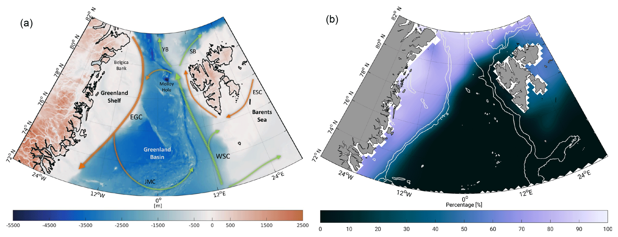
Figure 1Overviews of the study area: (a) bathymetry of the northern Nordic seas and Fram Strait area based on RTopo2 topography model (Schaffer et al., 2016). Arrows display major current systems (East Greenland Current, EGC; West Spitsbergen Current, WSC; East Spitsbergen Current, ESC; Jan Mayen Current, JMC; Yermak Branch, YB; and Svalbard Branch, SB). Light green arrows indicate inflowing Atlantic water; orange represents fresh polar and returning Atlantic water. (b) Averaged sea ice concentration in percentage within 2003–2009 based on 25 km monthly National Snow and Ice Data Center (NSIDC, Fetterer et al., 2017) sea ice concentration grids. White lines display depth contours at −450 and −1500 m. White areas indicate missing or flagged data.
The northern Nordic seas are characterized by contrasting water masses. Warm and salty waters of Atlantic origin are carried northward by the Norwegian Atlantic Current (e.g., Orvik and Niiler, 2002). After a bifurcation at the Barents Sea Opening, the remaining current that continues northward is termed the West Spitsbergen Current (WSC, e.g., Beszczynska-Möller et al., 2012; von Appen et al., 2016). A fraction of the Atlantic water carried by the WSC recirculates in the Fram Strait at around 79∘ N and continues to flow southward, forming the Return Atlantic Water (RAW), whereas the remaining part enters the Arctic Ocean via the Svalbard and Yermak branches (SB and YB). Along the Greenland continental shelf break, the East Greenland Current (EGC, e.g., de Steur et al., 2009) carries cold and fresh polar water as well as RAW southward.
Sea ice is exported via the Transpolar Drift out of the Arctic through the Fram Strait. As indicated in Fig. 1, the sea ice export occurs at the western side of the strait, which is thus ice-covered year-round. The eastern part of the Fram Strait is ice-free year-round due to the presence of warm Atlantic water. Around 10 % of the Arctic sea ice area is exported through the Fram Strait annually, an order of magnitude larger than the export through other Arctic gateways (Smedsrud et al., 2017).
2.2 Model basis: Finite Element Sea Ice-Ocean Model (FESOM)
In this study we use daily mean water level output from the Finite Element Sea Ice-Ocean Model (FESOM) version 1.4 (Wang et al., 2014; Danilov et al., 2015). FESOM is an ocean sea ice model which solves the hydrostatic primitive equations in the Boussinesq approximation. The sea ice component applies the elastic–viscous–plastic rheology (Hunke and Dukowicz, 2001) and thermodynamics following Parkinson and Washington (1979). The finite element method is used to discretize the governing equations, applying unstructured triangular meshes in the horizontal and z levels in the vertical. Water level heights (in the model labeled as sea surface height) η are computed from the following equation:
where is the velocity vector and H is the water depth. Water elevations are relative to a geopotential surface and therefore comparable to an altimetry-derived dynamic ocean topography (Androsov et al., 2018). The upper limit in the integration is set to zero, which corresponds to a linear free-surface approximation. This implies that the ocean volume does not change with time in the model. Thus, the model conserves volume but not mass. A correction for the global mean steric height change is not applied. To account for surface freshwater fluxes (precipitation, evaporation, river runoff, salinity changes due to sea ice melting and freezing), a virtual salt flux is introduced (see, e.g., Wang et al., 2014). The model does not take into account sea level pressure and ocean tide variations.
The global FESOM configuration used here was optimized for the Fram Strait, applying a mesh resolution of 1 km in the area 76–82.5∘ N, 20∘ W–20∘ E and a resolution of 4.5 km in the Nordic seas and Arctic Ocean (Wekerle et al., 2017). In the vertical, 47 z levels are used with a thickness of 10 m in the top 100 m and coarser vertical resolution with depth. The model bathymetry was taken from RTopo2 (Schaffer et al., 2016). For comparison, only the surface information is used (i.e., z=0).
The model is forced by atmospheric reanalysis data COREv.2 (Large and Yeager, 2008) characterized by a daily temporal and 2 ∘ spatial resolution, and interannual monthly river runoff is taken from Dai et al. (2009). Sea surface salinity restored to the PHC 3.0 climatology (Steele et al., 2001) is applied with a restoring velocity of 50 m per 300 days. The simulation covers the time period 2000 until 2009, and daily model output was saved. A comparison with observational data (e.g., moorings) revealed that the model performed well in simulating the circulation structure, hydrography and eddy kinetic energy in the Fram Strait (Wekerle et al., 2017).
2.3 Observational basis: radar altimetry data
In the present study high-frequency radar altimetry data of the ESA satellite Envisat are used. The altimeter emits radar signals in the Ku band with a footprint (i.e., circular area on the ground illuminated by the radar) of approximately 10 km diameter (Connor et al., 2009). Envisat belongs to the pulse-limited altimetry missions and provides observations characterized by a spatial along-track resolution of circa 372 m (18 Hz). The mission was placed in orbit in 2002 and provided altimetry data until the end of March 2012. This study uses high-frequency waveform data that are extracted from the official Sensor Geophysical Data Records (SGDR) version 2.1 provided by ESA. Data measured during the nominal mission period (May 2002–October 2010) are organized into 35-day repeat cycles including a fixed relative orbit number (i.e., pass, from pole to pole) of 1002 passes per cycle (ESA, 2011). However, the first cycles of Envisat are affected by various instrumental issues and are not considered for the present study. Considering the temporal availability of FESOM and reliable observations of Envisat, SGDR data of a period covering 7 complete years (2003–2009) are used. Before using the Envisat altimetry observations, a classification is performed to eliminate sea-ice-contaminated measurements. Sea surface heights (SSHs) are calculated by applying the ALES+ retracking algorithm (Passaro et al., 2018) and geophysical corrections. Unrealistic or bad height measurements are excluded by performing an outlier detection based on sea level anomalies. Finally, a transformation to physical heights (dynamic ocean topography, DOT) is processed by subtracting geoid heights from SSH. The following subsections describe the individual preprocessing steps in more detail.
2.3.1 Sea ice and water discrimination
Most of the Arctic regions are affected by seasonal sea ice cover, which can prevent a reliable estimation of sea surface heights due to a direct impact on the reflected radar pulses. In order to overcome this difficulty and to allow for a SSH comparison with FESOM, a classification is performed to detect small open water gaps (e.g., leads, polynyas) within the sea-ice-covered area. For this purpose an unsupervised classification approach (i.e., without the use of any training data) based only on radar waveforms and derived parameters is applied. Several classification methods have been developed within the last years, which are all based on the analysis of the returned satellite radar echo (e.g., Laxon, 1994; Zakharova et al., 2015; Zygmuntowska et al., 2013). Most of them impose thresholds on one or more parameters of the radar waveforms (e.g., maximum power or backscatter coefficient). In this study, an unsupervised classification approach is applied, which is independent of any training data. This method performed best in a recent study assessing the quality of different classification approaches with respect to very high resolution airborne imagery (Dettmering et al., 2018). Briefly summarized, the unsupervised classification approach, described by Müller et al. (2017), groups an unassigned subset of altimetry radar waveforms into a predefined number of classes by applying a partitional cluster algorithm (i.e., k-medoids; see Celebi, 2015) in order to establish a reference waveform model to indicate different waveform and surface characteristics. In the following step, the generated waveform model acts as kind of assignment map for the remaining waveforms, which are allocated to the particular classes using a simple k-nearest-neighbor classifier. Further information and explanations can be found in Müller et al. (2017). The open water (leads, polynyas and open ocean) observations are used for all following processing steps. Measurements classified as ice are removed from the dataset. However, it has to be noted that some misclassifications, e.g., due to the presence of fast ice, can still remain in the observation dataset (Müller et al., 2017). During sea ice melt season, melt ponds and water bodies on top the sea ice layer can cause uncertainties in the computation of sea surface heights. The unsupervised classification is not fully tuned to discriminate carefully between radar waveforms originating from melt ponds or leads at the sea surface level. In the case of misclassification the estimated altimeter ranges can appear too short.
2.3.2 Sea surface height estimation
SSH is obtained by subtracting the measured range between satellite and water surface (including geophysical corrections) from the orbital altitude (i.e., ellipsoid height) of the satellite's center of mass. The range can be calculated by fitting a waveform model (e.g., Brown, 1977, or Hayne, 1980) to the individual radar returning signals. More information regarding retracking strategies can be found for example in Vignudelli et al. (2011). Several retracking algorithms have been developed and optimized for special applications, surface conditions or study regions (e.g., open ocean, sea ice or inland water bodies). According to Serreze and Barry (2014) the northern Nordic seas are characterized by rapidly changing environmental conditions, making it difficult to use just one retracking algorithm. However, when combining heights derived with different retrackers, systematic offsets due to different retracker biases will be introduced (Bulczak et al., 2015). The usage of ALES+ overcomes this problem by adapting a subwaveform application of the classic open ocean functional form to different shapes of the radar signals, including the typical peaky signal shape of the returns from small leads and corrupted trailing edges typical of coastal waveforms. Passaro et al. (2018) have developed and tested the algorithm against standard open ocean and lead retrackers and showed improvements in precision and in terms of comparison with a local tide gauge. The algorithm was used to develop Arctic and Antarctic products in the framework of the ESA Sea Level Climate Change Initiative (Legeais et al., 2018).
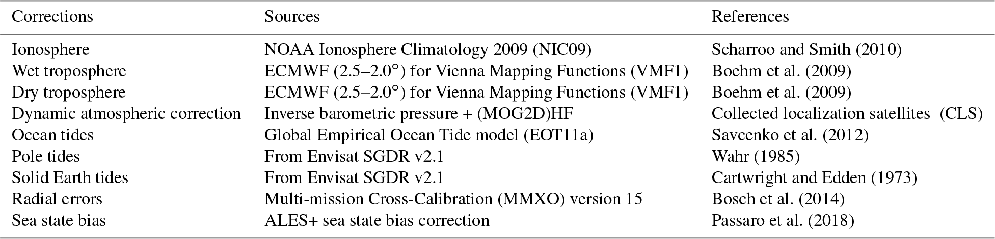
After the retracking, the altimeter ranges are corrected for geophysical and atmospheric effects using external model data. Wind and wave effects are considered by using the sea state bias estimates of the ALES+ retracking approach. Furthermore a mean range bias correction, computed by a multi-mission crossover analysis (Bosch et al., 2014), is included to eliminate a known constant offset in the Envisat range measurements. One important correction is the ocean tide correction since the FESOM model does not include ocean tides. In this study, we use EOT11a (Savcenko et al., 2012; Savcenko and Bosch, 2012) to correct for tidal effects. Even if EOT11a is a global ocean tide model it performs reasonably well in the Arctic Ocean (Stammer et al., 2014). This study performs a validation by comparing different tide models to tide gauge data. For the Arctic Ocean, EOT11a shows rms values between 1.4 and 4.6 cm for the four major constituents, and it is the second best of the seven models in the test. Table 1 lists all corrections used within the present investigation.
Scharroo and Smith (2010)Boehm et al. (2009)Boehm et al. (2009)Collected localization satellites (CLS) (2016)Savcenko et al. (2012)Wahr (1985)Cartwright and Edden (1973)Bosch et al. (2014)Passaro et al. (2018)Table 1Geophysical and empirical altimetry corrections applied in the study.
To remove erroneous and unreliable sea surface height observations from the dataset, an outlier rejection is performed by applying a fixed threshold criterion. The SSH observations are compared to a long temporal mean sea surface (MSS), including more than 20 years of altimetry data, and sea level anomalies (SLAs) are built. The conversion is done by removing the DTU15MSS developed by Andersen and Knudsen (2009) from the along-track sea surface heights. Without being too restrictive within the sea ice zones with a higher noise level than in open ocean, a threshold of ±2 m is introduced. This rejects 1.54 % of the high-frequency measurements of Envisat. After removing outliers the revised dataset is retransformed to sea surface heights by re-adding the MSS.
2.3.3 Dynamic ocean topography estimation
After obtaining sea surface heights the transition to physical heights is performed with respect to an underlying geoid model (i.e., the computation of DOT). In the present investigation the high-resolution Optimal Geoid Model for Modeling Ocean Circulation (OGMOC), developed up to a harmonic degree of 2190 and corresponding to a spatial resolution of nearly 9.13 km, is applied. This is one of the latest high-resolution global geoid models incorporating the most recent satellite gravimetry and satellite altimetry datasets. Moreover it is optimized for estimating ocean currents and it is assumed to provide the best possible solution for the current application. More details regarding to the constituents and processing strategy of the geoid can be found in Gruber and Willberg (2019) and Fecher and Gruber (2018). Briefly summarized, OGMOC is a combination of XGM2016 (Pail et al., 2018) and the EIGEN6-C4 model (Förste et al., 2004). XGM2016 is used up to degree 619. Between 619 and 719, XGM2016 and EIGEN6-C4 are combined applying a weighting function. Higher harmonic degrees (>719) are retained unchanged from the EIGEN6-C4 model.
To minimize noise within the high-frequency altimetry database and to be more consistent with the spatial resolution of the geoid, the corrected along-track SSH observations get low-pass filtered by applying a moving average using a rectangle kernel adapted to the spatial resolution of the used geoid (9.13 km). Areas with sparse availability of along-track observations (e.g., leads, polynyas) less than the window size are not considered in the filtering process and remain unfiltered in the dataset. The DOT is derived by interpolating the geoid heights to the altimetry locations and subtracting them from the SSH observations.
The preprocessed ocean heights from altimetry and FESOM are compared with each other to identify similarities and discrepancies and to explore the possibility of a combination. Therefore, in the first step, both datasets are analyzed and examined regarding their temporal and spatial characteristics. The datasets are investigated in terms of constant offsets, seasonally occurring patterns (e.g., annual sea level variability) and residual sea level variations.
The FESOM data are provided on daily unstructured grids with local refinements in the central Greenland Sea and the Fram Strait. In contrast, the altimetry observations are sampled along-track and characterized by a high spatial resolution with irregular data gaps due to sea ice coverage. Figure 2 displays the inhomogeneously distributed FESOM nodes showing a maximum resolution of about 1 km. Moreover, three representative days of altimetry along-track data are shown with different behavior in observation availability depending on the season and the presence of sea ice. During the sea ice maximum in March (Kvingedal, 2013) most of the altimetry data close to the Greenland coast are missing due to a semi-closed sea ice cover. In contrast, in the summer season the tracks show fewer data gaps.
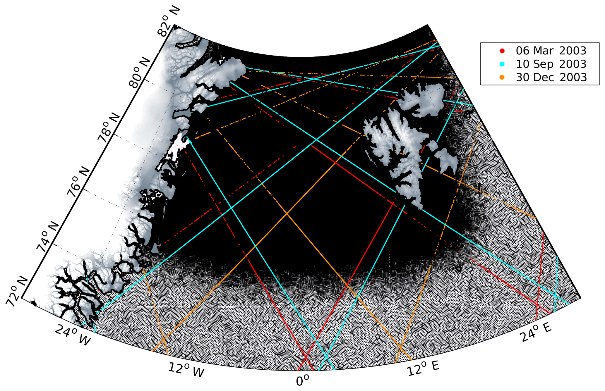
Figure 2Locations of selected altimetry observations in wintertime and summertime. The small black dots indicate the unstructured FESOM grid nodes migrating at higher latitudes to a apparently closed black background.
In order to allow a direct and pointwise comparison of both datasets, a resampling of at least one of them is necessary. Since the FESOM data exhibit a significantly higher spatial and a uniform temporal resolution, they will be interpolated using a nearest-neighbor algorithm with the times and locations of the altimetry observations. This prevents an unnecessary smoothing of the altimetry data.
3.1 Assessment of the annual cycle
It can be expected that the annual sea level variability is the dominant signal contained in both datasets (e.g., Bulczak et al., 2015). The present analysis performs a comparison of the annual and remaining temporal signal components within the investigation period by fitting harmonic functions to both datasets.
In the first step, daily height averages for the entire region are computed. Figure 3 shows the temporal evolution of the daily means within the investigation period for both datasets. An obvious offset of about 41 cm between the datasets caused by different underlying height references (geoid vs. bathymetry) is clearly visible. Furthermore, a linear trend or another long-term systematic behavior is not detectable, probably due to the short period of only 7 years. However, the altimetry-derived daily averaged DOT shows larger variations and a standard deviation of 9.0 cm. In contrast, the modeled data are characterized by a smoother behavior and a smaller standard deviation of 4.7 cm. These numbers include a clear seasonal cycle, which is also clearly visible in Fig. 3.
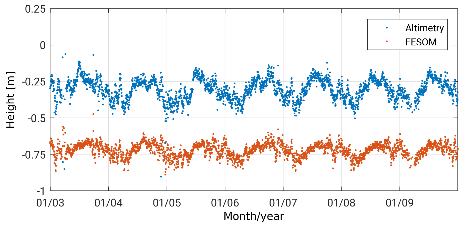
Figure 3Temporal evolution of daily means of altimetry-derived DOT observations (blue) and FESOM SSH outputs (interpolated to the locations of altimetry measurements, red) within the investigation period and study area (see Sect. 2).
In order to examine both datasets concerning their annual period, the daily means are analyzed by a Fourier analysis (e.g., Stade, 2005). Therefore, both time series are centered at zero by reducing their constant offsets before the Fourier coefficients are obtained by applying a least-squares estimation (e.g., Thomson and Emery, 2014).
Figure 4a displays the amplitude spectrum of the interpolated FESOM and profiled altimetry daily means between 2003 and 2009. The modeled data are characterized by weaker amplitudes. The annual period constitutes the most dominant long-period signal. In the case of altimetry, the annual amplitude represents 6.9 cm and, in the case of FESOM, 3.9 cm of the sea level variability. Other frequencies can not be physically explained and thus are not further investigated in the present study. In particular, the semiannual signal is very small (1.5 cm) and shows no significant impact on both datasets. The remaining amplitudes are smaller than 1.5 cm in the case of altimetry (1.0 cm, FESOM).
However, an amplitude of almost 2 cm is detectable for a period of 3 days, which cannot be assigned to ocean or sea-ice-related dynamics. This is an artifact possibly caused by the irregular data sampling. In order to prove this hypothesis, the frequency analysis is also performed for the full FESOM grid. Figure 4b shows the amplitude spectrum and the estimated periods for the daily profiled FESOM DOT (red) and the original FESOM DOT (black). It can be clearly observed that the 3-day period is not confirmed by the original dataset. Moreover, higher discrepancies can be found in the short periodic domain, which can be attributed to more variability due to more input information. However, all other dominant periods are caught by both datasets. The obtained amplitudes show good agreement in all periods except for the annual signal. Here, the irregularly sampled profile data overestimate the amplitude by about 1 cm. This might be related to alias effects from remaining tidal influence due to the repeat cycle of Envisat (see Sect. 4 for more details).
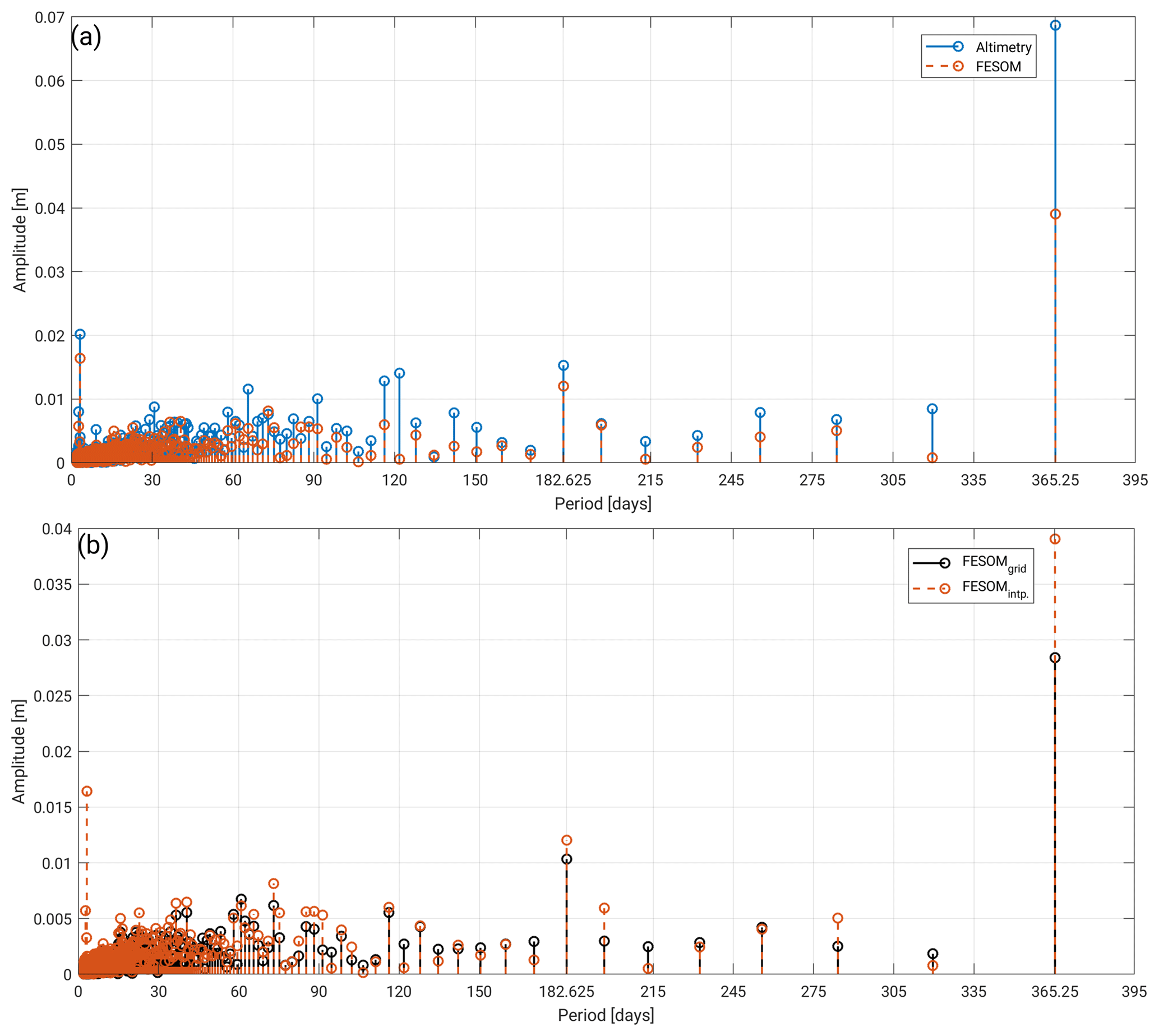
Figure 4Fourier analysis amplitude spectrum of two altimetry locations interpolated with FESOM data (red) from (a) altimetry-derived DOT along-track observations (blue) and (b) original FESOM data (black) within the investigation area from 2003 to 2009 (see Sect. 2).
As mentioned earlier the annual signal represents the most dominant signal in both datasets. By introducing the obtained annual Fourier coefficients to a harmonic fitting, the temporal evolution and the phasing can be shown (see Fig. 5). Aside from differences in the annual amplitudes, a phase shift of about 29 days is recognizable between the two signals. The maximum is reached at day of year (DOY) 230 (18 August) for altimetry and in the case of FESOM at DOY 259 (16 September).
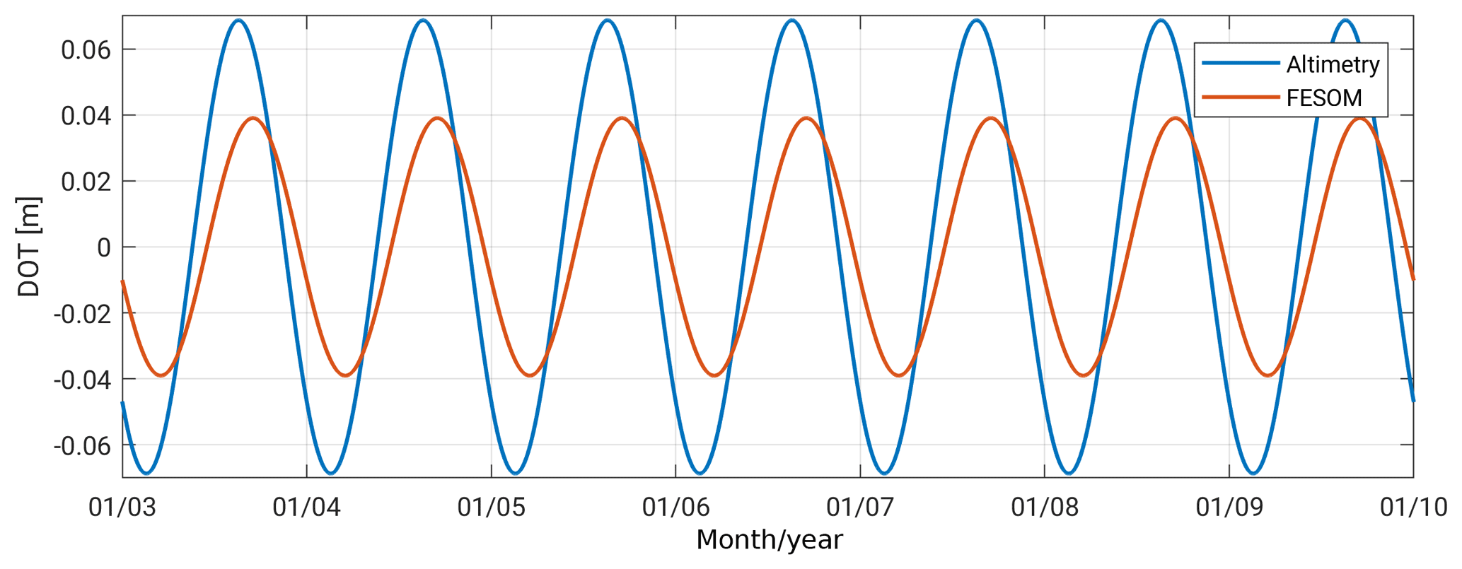
Figure 5Annual cycles of DOT from along-track altimetry (blue) observations and FESOM (red) simulations within the investigation time and area (see Sect. 2).
However, it is obvious that one single harmonic function cannot represent the full complexity of the DOT variations in the northern Nordic seas. A detailed analysis of the annual signal considering different bathymetric features (e.g., shelf or deep sea areas) brings the opportunity to estimate region-dependent annual amplitudes and phases. This is presented in the following section.
3.2 Spatiotemporal pattern analysis
In order to analyze regionally dependent differences, the profiled altimetry data are monthly averaged and arranged into along-track bins of 7.5 km length. The bin structure follows the nominal 1 Hz ground track pattern of Envisat and reduces the high-frequency measurement noise. Enabling long-term analyses, only satellite passes are admitted showing an availability of at least 64 repeat cycles, which corresponds to 96 % of the data in the evaluation period. Data gaps or missing bins are possible due to sea ice contamination or failing observations. For FESOM, daily data from the closest grid node are assigned to each bin. Thus, this dataset exhibits the same spatial resolution but a better temporal resolution, allowing for a more precise amplitude estimation.
Figure 6 displays for each bin the estimated annual DOT variations within 2003–2009. The amplitudes of both datasets show a similar pattern with smaller values along the major current systems (EGC and WSC) and larger values along the Greenland and Svalbard coasts and in the area around the Molloy Hole. In general, the altimetry-derived amplitudes are larger than the model amplitudes. In the Greenland Basin, a 2–3 times stronger representation of the annual amplitudes can be observed. Here, the mean altimetry amplitude reaches 6.3 cm. In the southern and eastern parts of the shelf regions, the altimetry amplitudes are smaller than the model amplitudes.
The maximum amplitudes in the Greenland Basin appear during August and September and show a mostly homogeneous distribution in both datasets. In ice-free regions both datasets show good agreement (also in comparison with results of Volkov and Pujol, 2012, and Mork and Øystein Skagseth, 2013). However, in ice-covered shelf regions, the central Fram Strait and close to calving glaciers, the derived amplitudes differ up to 8 cm. The altimetry estimated annual maximum on the Greenland Shelf occurs in November, which is confirmed by FESOM. Nevertheless, obvious phase differences between FESOM and altimetry can be found east of Spitsbergen, where the observed annual maximum occurs in the early spring months, in contrast to FESOM displaying a maximum in autumn. This could perhaps be caused by sea ice interference or strong ocean variabilities.
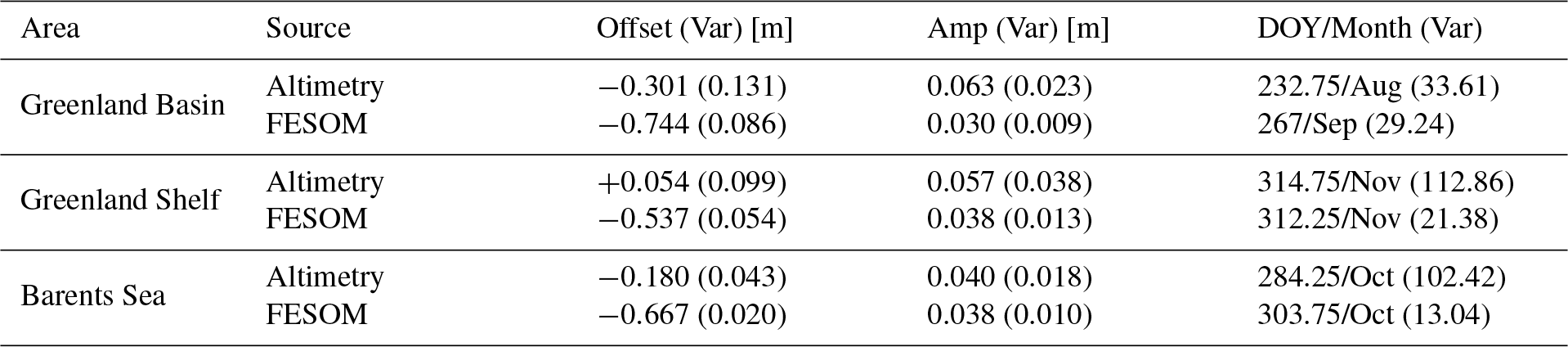
In order to account for different hydrological (e.g., glacier melt, water mass changes), atmospheric (e.g., winds, solar radiation) and oceanographic effects (e.g., ocean currents) in the study area, the region is subdivided into three main subareas: the deep basin region (Greenland Basin, m) and two shelf regions (Greenland Shelf, Barents Sea). Table 2 provides outlier-removed (3σ criterion) mean amplitudes and DOYs of the maximum amplitude for the three subregions, as well as their annual variabilities. FESOM shows similar amplitudes for all three areas, whereas altimetry exhibits smaller mean amplitudes for the Barents Sea than for the two other regions, where the mean amplitudes are about twice the amplitudes of FESOM. The phase shows good consistency between altimetry and FESOM on the Greenland Shelf but discrepancies of circa 34.25 days in the Greenland Basin and 19.5 days in the Barents Sea. A discussion of the differences is provided in Sect. 4.
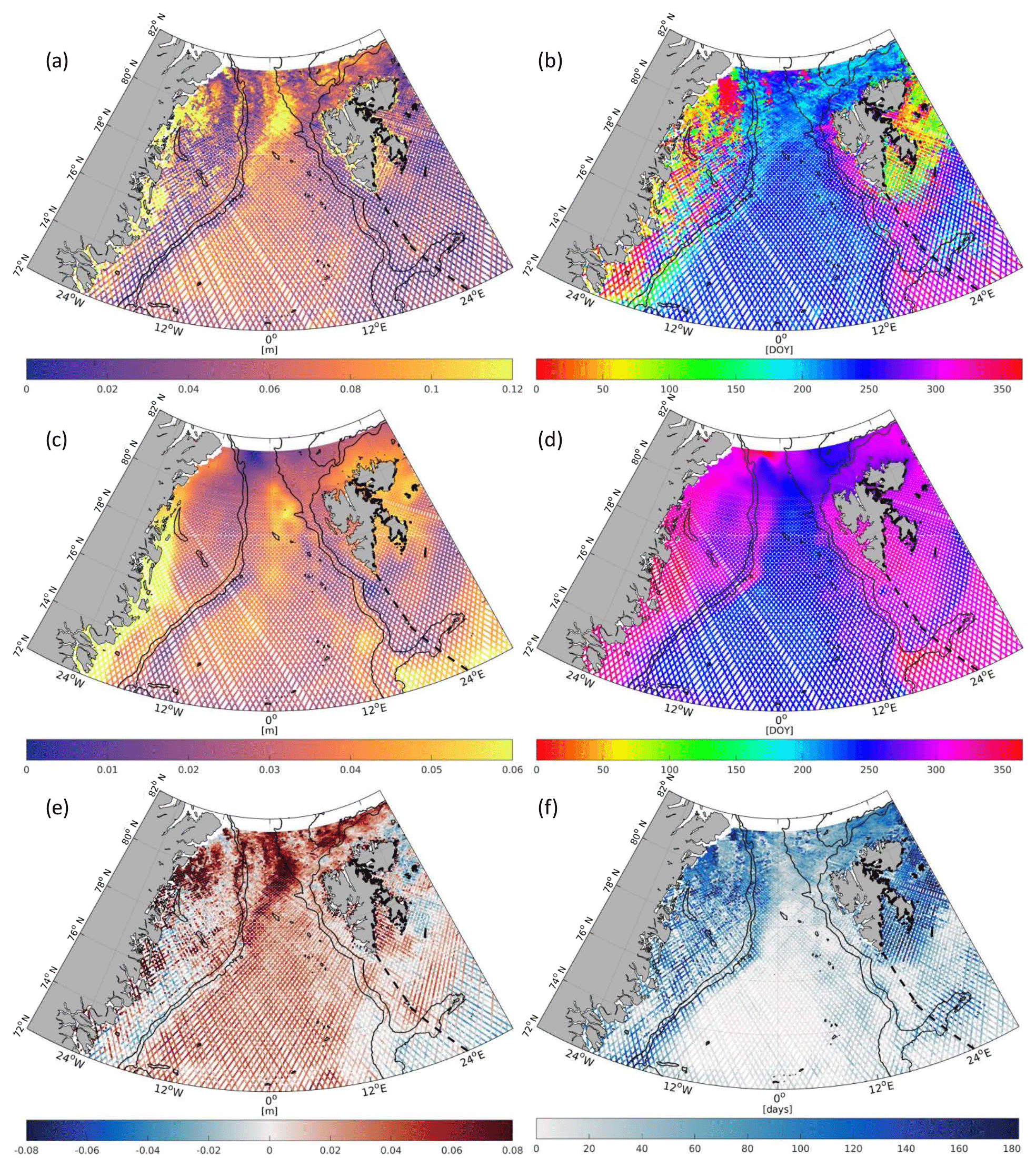
Figure 6Mean annual amplitudes (a, c, e) and the day of year (DOY) of the annual maximum (b, d, f) per bin for altimetry (a, b) and FESOM (c, d) DOT heights. The bottom row (e, f) displays amplitude (in m) and phase differences (in days) of altimetry minus FESOM. RTopo2 bathymetric contours (black) indicate the shelf (−450 m) and the basin (−1500 m) regions. The dashed lines highlight the Barents Sea boundary (IHO, International Hydrographic Organization, 1953). Note the different scales of the amplitude color bars.
Table 2Offset, averaged annual amplitude (Amp) and DOY/month of maximum amplitude with variability (Var) in three subregions.
3.3 Residual analysis
In order to analyze residual differences, both datasets are reduced by their regional estimated annual signal and constant offsets as given in Table 2. Figure 7 shows monthly averaged along-track residual DOT for altimetry and FESOM for the three study regions. In all areas, a high correlation between the datasets is visible. For the Greenland Basin and the Barents Sea, almost no systematic effects are detectable, whereas the altimetry time series for the Greenland Shelf exhibits multi-annual anomalies that are less pronounced in the FESOM time series, which only shows a small, insignificant behavior trends. However, the investigation period is too short to allow for a reliable interpretation of the underlying effects.
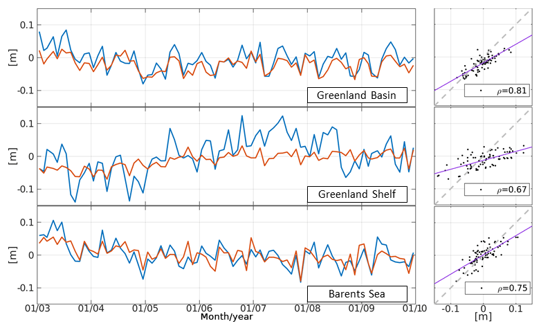
Figure 7Monthly time series of averaged residual heights from altimetry (blue) and FESOM (red). Offsets and annual signals were removed for each region. Additionally, scatter plots and correlation (ρ) are displayed. Regression and bisectrix lines are shown by the purple and dashed gray lines, respectively.
Figure 8 shows the geographical distribution of the mean residual signals and weighted average of standard deviation per bin. Both datasets display similar spatial patterns. However, obvious differences can be seen in some areas, e.g., the central Fram Strait and the transition areas between the deep basin and shelf regions. Comparing the variability of the residuals, the altimetry-derived DOT shows in general higher values and an enhanced variations in the ice-covered shelf areas, contrary to FESOM displaying more variability in regions affected by ocean currents.
Figure 9 shows the differences between the averaged residual DOT of altimetry and FESOM (left) as well as their correlation per bin (right). The largest differences occur on the northern Greenland Shelf and in the Fram Strait, whereas fewer sea-ice-affected areas (e.g., Greenland Basin, Barents Sea), including the current and eddy regions (e.g., WSC), show good agreement. The correlations are mainly positive, with values above 0.5 % for 21 % of the bins. High positive correlations are displayed in the deep basin parts of the study area. Smaller positive correlations can be found in regions with strong bathymetric gradients and in northern areas of the major ocean currents (e.g., WSC, EGC).
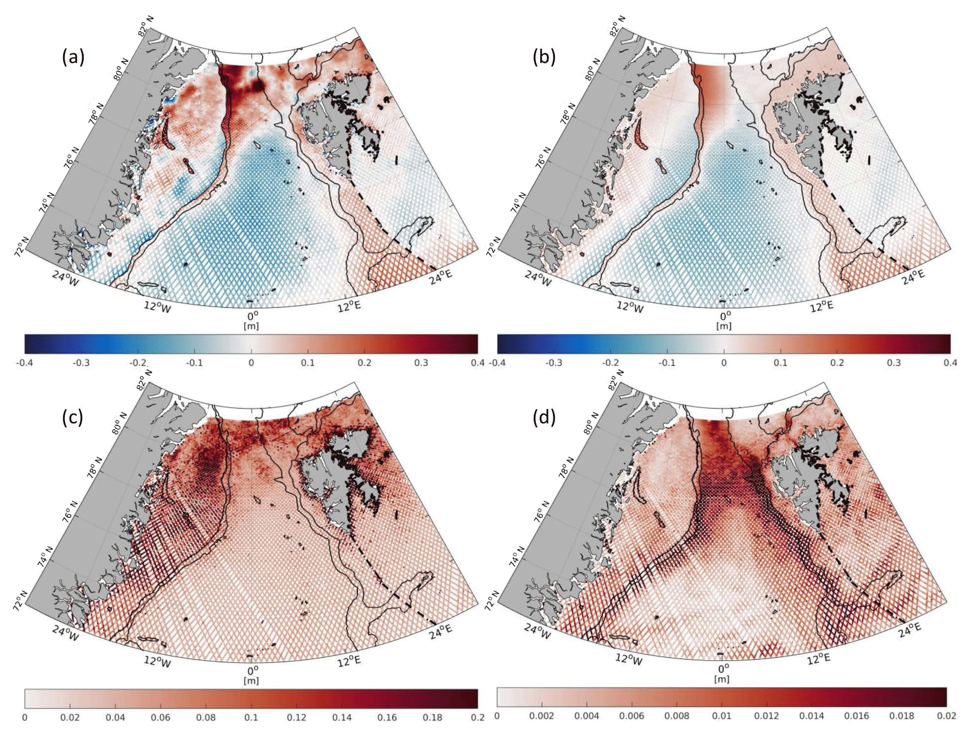
Figure 8Weighted mean residual DOT (a, b) and weighted mean of standard deviation (c, f) for each bin from altimetry (a, c) and FESOM (b, d) within 2003–2009. Note the different scales of standard deviation color bars.

Figure 9Differences (a) and correlations (b) between altimetry and FESOM binned along-track residual DOT within the investigation period.
Remarkable elevation differences occur between 80 and 82∘ N. These patterns are seen in the altimetry-derived DOT but not in the model and yield up to 0.4 m. They show a constant behavior within the entire investigation period, which cannot be attributed to seasonal ocean phenomena. Instead, these artifacts are due to geoid errors caused by residual ocean signals at polar latitudes (e.g., Kwok and Morison, 2015; Farrell et al., 2012). More discussion related to the geoid can be found in the next section.
The comparison of the altimetry-derived and simulated DOT shows good agreement in terms of highly correlated regional time series and small residual heights. Predominately positive correlations between both datasets can be found in ice-free areas (e.g., Greenland Basin) and in regions affected by ocean currents. FESOM and altimetry display a very similar frequency behavior for the most dominant periodic DOT variability. In comparison with previous studies, the along-track altimetry DOT agrees concerning annual amplitudes and phases as obtained by Volkov and Pujol (2012) and Mork and Øystein Skagseth (2013).
However, the analysis also reveals some systematic discrepancies. These can be explained by three different error sources: they partly originate from modeling errors of FESOM, partly from measurement uncertainties of altimetry and partly from errors of the geoid used for computing the altimetry DOT. These points will be discussed in more detail in the following paragraphs.
FESOM is affected by synthetic smoothing due to the added numerical diffusion component stabilizing the model runs and preventing the simulated DOT from uncontrolled variabilities. Moreover, in the present investigation the FESOM run does not include the latest glacier runoff model, which causes further irregularities close to northeastern Greenland's coast. Another reason causing this smoothing effect can be found in the too strongly adjusted sea ice friction coefficient of the model, damping DOT variabilities in sea-ice-affected regions. The model applies strictly the hydrostatic equations, which function as an assumption of the real sea state. Furthermore, it does not include tidal ocean signal and barometric effects and lacks a steric correction to ensure the global conservation of mass.
While the first two points are taken into account by correcting the altimetry observations, the latter point is currently not considered in the comparison. This should be acceptable since the impact on low-frequency regional sea level patterns is small (Griffies and Greatbatch, 2012). However, it will contribute to the constant and long-term differences visible in this study. In contrast, remaining differences in handling the atmospheric sea level pressure (i.e., caused by uncertainties of the used correction model) will show up in regional differences. They might be the reason for the observed temporal shifts of the maximum annual signal in the Greenland Basin. Even more important is the insufficiently realistic consideration of freshwater inflow (e.g., by glacier runoff) by FESOM. This can cause phase shifts as well as reduced annual amplitudes. Furthermore the coarse resolution of atmospheric forcing is an additional reason for a smoothed sea level representation and an underestimation of annual amplitudes.
For satellite altimetry, the polar oceans are a challenging region, especially when sea ice is present. In these areas, the returned radar echoes are comprised of signals from different surface reflectors such as different ice types and structures, melt ponds on ice and open water. The challenge is to extract valuable information about the sea level while disregarding all other reflectors. Even with the application of a dedicated waveform classification and special retracking, as performed here, DOT estimates in coastal and sea ice areas are significantly more noisy than in open ocean. Moreover, the applied range corrections can be biased by the Arctic Ocean conditions, leading to more unreliable range estimations in ice-covered shelf regions. Thus, in these regions, small-scale structures are not thoroughly reliable.
Due to its measurement geometry, satellite altimetry has a high along-track resolution, but data are scattered in time and space. In addition, in polar regions, an irregular sampling due to missing data caused by sea ice coverage must be taken into account. This can significantly influence the estimation of annual sea level variability, as tests with simulated data with different sampling revealed (see Sect. 3.1).
However, an interpolation of the dataset as it is done in the majority of other studies (e.g., Kwok and Morison, 2015; Armitage et al., 2016; Farrell et al., 2012) could be avoided in order to conserve more high-frequency observations and spectral content.
This study is based on data from Envisat, whose repeat cycle is known to cause severe alias effects of 365 days for the tidal constituents K1 and P1 (see Volkov and Pujol, 2012, and Padman et al., 2018). Thus, errors in K1 and P1 in the applied ocean tide model may impact the estimated annual variation of the altimetry-based DOT. Passaro et al. (2015) showed that the effect can reach up to 1–3 cm. For this study, the EOT11a ocean tide model (Savcenko et al., 2012) is used. Even if that model is proven to be among the best models of the Arctic Ocean (see Stammer et al., 2014) the differences between FESOM and altimetry in the bin-wise estimated annual amplitudes could be partially attributed to this aliasing effect. However, the analysis presented in Sect. 3.1, which is based on averaged Envisat data, also shows a discrepancy of more than 1 cm between FESOM and altimetry amplitudes. Thus, the majority of this difference will be due to the smoothing effect of FESOM.
In addition to simulated and observational data irregularities, stationary artifacts caused by geoid inaccuracies can be clearly identified in the northern Fram Strait region. Following Kwok and Morison (2015) these synthetic looking elevations in the altimetry-derived DOT can be attributed to a combination of geoid residuals and oceanographic features, which are very challenging to separate from each other. A significant problem can be seen in the specific components of the geoid models. The higher spherical harmonics (degrees 720–2190), describing shorter wavelength patterns (10–30 km), are based on selective in situ and satellite altimetry gravity observations, which can be contaminated by sea ice or feature sparse availability. Within this study, one of the newest geoid models is used, which has been developed for ocean circulation studies and has been optimized to avoid striations and orange skin-like features. Nevertheless, it seems to contain the remaining artificial structures in the study area. According to Gruber and Willberg (2019), the higher spherical harmonics are covered by EIGEN6-C4 geoid model (Förste et al., 2004), which does not include current satellite altimetry data. However, mid spherical harmonic degrees, corresponding to a 30–100 km spatial wavelength, are represented by XGM2016 (Pail et al., 2018) including the latest altimetry marine gravity fields. Hence, a better representation of short wavelength patterns can only be reached by introducing the latest and updated altimetry data, supported by in situ measurements of the geoid computations. Similar effects are also visible when using alternative geoid models (Skourup et al., 2017).
In the present paper, high-frequency altimetry-derived DOT is compared with water elevations of FESOM in order to identify their similarities and discrepancies as well as their respective benefits. Both datasets are characterized by different limitations, which prevent a perfect representation of the dynamic topography in polar regions based on only one approach. The present investigation demonstrates that model simulations and observations are both needed to understand the complexity of ocean processes in the polar latitudes, especially in the Arctic Ocean.
The present paper shows basic agreement between a numerically simulated and an empirical estimated representation of the DOT in the northern Nordic seas in terms of annual variability and spatial behavior. However, inconsistencies due to the higher noise level of the observations, especially in sea ice areas, and the enhanced smoothing of the model are demonstrated. For example, an offset of about half a meter exists between the two datasets since the data of FESOM are not defined with respect to a standard reference frame (Androsov et al., 2018). Moreover, the annual sea level variability observed by the two datasets differs by a few centimeters. The residual heights show a similar pattern, high temporal correlations and only small differences, which are mainly related to sea ice coverage and geoid artifacts.
The results presented in this paper indicate that further improvements can be made to both datasets: the altimetry-derived DOT still needs a better or more restrictive handling of sea ice observations as well as a more reliable Arctic geoid. FESOM should be corrected for a global mean steric height change (Greatbatch, 1994) in order to ensure the conservation of mass and to make the observed altimetry heights directly comparable to the model heights. In addition, an improved handling of freshwater inflow is required to better account for mass changes due to glacier as well as river runoff.
However, even if these points will be improved, the principal limitations of observations (measurement noise and data gaps in regions with closed sea ice coverage) and models (absolute height level) will persist. Thus, it seems reasonable to exploit the advantages of both datasets through a combination of model and along-track observations. This will enable the derivation of a homogeneous DOT, equally sampled in time and space without the need of smoothing the altimetry measurements by gridding procedures. In such an approach, the absolute level as well as the annual variability of altimetry should be preserved, and the continuous spatial representation of the model should be used to bridge regions influenced by sea ice coverage and to get rid of unreliable high-latitude geoid artifacts. This will allow for an optimized determination of the Arctic DOT and the associated surface currents. Concerning the current availability of altimetry-derived DOT estimations, it is possible to establish a combination of simulated and observation-based DOT representation covering more than 25 years, enabling climate-relevant conclusions.
Envisat RA2 altimetry data access is available from ESA after fast registration submission (https://doi.org/10.5270/EN1-85m0a7b, ESA, 2018). The FESOM data can be requested from Alfred Wegener Institute. A final combined data product will be provided via PANGAEA (https://www.pangaea.de/, last access: 13 February 2019) once the project is completed.
FLM developed the comparison methods, conducted the data analysis and wrote the majority of the paper. CW provided the FESOM data and contributed to the manuscript writing. DD supervised the present study, contributed to the manuscript writing and helped with discussions of the results. MP developed the retracking algorithm and helped with the application and discussion concerning the altimetry dataset. WB initiated the study. FS supervised the research.
The authors declare that they have no conflict of interest.
The authors thank the ESA for operating Envisat and for supplying the SGDR v2.1
dataset. The authors thank the Chair of Astronomical and Physical Geodesy,
Technical University of Munich (TUM), for providing the geoid model, OGMOC.
This work was mainly supported by the German Research Foundation (DFG)
through grants BO1228/13-1, DE2174/3-1 and in part through grant OGreen79
as part of the Special Priority Program (SPP)-1889 ”Regional Sea Level Change
and Society” (SeaLevel). We thank Sine M. Hvidegaard
and two further anonymous reviewers for their valuable comments that helped
to improve the manuscript.
This work was supported by the German Research Foundation (DFG) and the
Technical University of Munich (TUM) in the framework of the Open Access
Publishing Program.
Edited by: David M. Holland
Reviewed by: Sine M. Hvidegaard and two anonymous referees
Andersen, O. B. and Knudsen, P.: DNSC08 mean sea surface and mean dynamic topography models, J. Geophys. Res.-Oceans, 114, c11001, https://doi.org/10.1029/2008JC005179, 2009. a
Androsov, A., Nerger, L., Schnur, R., Schröter, J., Albertella, A., Rummel, R., Savcenko, R., Bosch, W., Skachko, S., and Danilov, S.: On the assimilation of absolute geodetic dynamic topography in a global ocean model: impact on the deep ocean state, J. Geodesy, 1–17, https://doi.org/10.1007/s00190-018-1151-1, 2018. a, b
Armitage, T. W. K., Bacon, S., Ridout, A. L., Thomas, S. F., Aksenov, Y., and Wingham, D. J.: Arctic sea surface height variability and change from satellite radar altimetry and GRACE, 2003–2014, J. Geophys. Res.-Oceans, 121, 4303–4322, https://doi.org/10.1002/2015JC011579, 2016. a, b
Beszczynska-Möller, A., Fahrbach, E., Schauer, U., and Hansen, E.: Variability in Atlantic water temperature and transport at the entrance to the Arctic Ocean, 1997–2010, ICES J. Mar. Sci., 69, 852–863, https://doi.org/10.1093/icesjms/fss056, 2012. a
Boehm, J., Kouba, J., and Schuh, H.: Forecast Vienna Mapping Functions 1 for real-time analysis of space geodetic observations, J. Geodesy, 83, 397–401, https://doi.org/10.1007/s00190-008-0216-y, 2009. a, b
Bosch, W., Dettmering, D., and Schwatke, C.: Multi-Mission Cross-Calibration of Satellite Altimeters: Constructing a Long-Term Data Record for Global and Regional Sea Level Change Studies, Remote Sens., 6, 2255–2281, https://doi.org/10.3390/rs6032255, 2014. a, b
Brown, G.: The average impulse response of a rough surface and its applications, IEEE T. Antenn. Propag., 25, 67–74, https://doi.org/10.1109/TAP.1977.1141536, 1977. a
Bulczak, A. I., Bacon, S., Naveira Garabato, A. C., Ridout, A., Sonnewald, M. J. P., and Laxon, S. W.: Seasonal variability of sea surface height in the coastal waters and deep basins of the Nordic Seas, Geophys. Res. Lett., 42, 113–120, https://doi.org/10.1002/2014GL061796, 2015. a, b
Cartwright, D. E. and Edden, A. C.: Corrected Tables of Tidal Harmonics, Geophys. J. Int., 33, 253–264, https://doi.org/10.1111/j.1365-246X.1973.tb03420.x, 1973. a
Celebi, M.: Partitional Clustering Algorithms, EBL-Schweitzer, Springer International Publishing, https://doi.org/10.1007/978-3-319-09259-1, 2015. a
Collected localization satellites (CLS): Dynamic atmospheric Corrections are produced by CLS Space Oceanography Division using the Mog2D model from Legos and distributed by Aviso+, with support from Cnes, AVISO+, available at: http://www.aviso.altimetry.fr, last access: 28 November 2016. a
Connor, L. N., Laxon, S. W., Ridout, A. L., Krabill, W. B., and McAdoo, D. C.: Comparison of Envisat radar and airborne laser altimeter measurements over Arctic sea ice, Remote Sens. Environ., 113, 563–570, https://doi.org/10.1016/j.rse.2008.10.015, 2009. a, b
Dai, A., Qian, T., Trenberth, K. E., and Milliman, J. D.: Changes in Continental Freshwater Discharge from 1948 to 2004, J. Climate, 22, 2773–2792, https://doi.org/10.1175/2008JCLI2592.1, 2009. a
Danilov, S., Wang, Q., Timmermann, R., Iakovlev, N., Sidorenko, D., Kimmritz, M., Jung, T., and Schröter, J.: Finite-Element Sea Ice Model (FESIM), version 2, Geosci. Model Dev., 8, 1747–1761, https://doi.org/10.5194/gmd-8-1747-2015, 2015. a
de Steur, L., Hansen, E., Gerdes, R., Karcher, M., Fahrbach, E., and Holfort, J.: Freshwater fluxes in the East Greenland Current: A decade of observations, Geophys. Res. Lett., 36, 23, https://doi.org/10.1029/2009GL041278, 2009. a
Dettmering, D., Wynne, A., Müller, F. L., Passaro, M., and Seitz, F.: Lead Detection in Polar Oceans – A Comparison of Different Classification Methods for Cryosat-2 SAR Data, Remote Sens., 10, 1190, https://doi.org/10.3390/rs10081190, 2018. a
ESA: Envisat Altimetry Level 2 User Manual V 1.4, European Space Agency (ESA), October, 2011. a
ESA: RA-2 Sensor and Geophysical Data Record – SGDR, European Space Agency, https://doi.org/10.5270/en1-85m0a7b, 2018. a
Farrell, S. L., McAdoo, D. C., Laxon, S. W., Zwally, H. J., Yi, D., Ridout, A., and Giles, K.: Mean dynamic topography of the Arctic Ocean, Geophys. Res. Lett., 39, 1, https://doi.org/10.1029/2011GL050052, 2012. a, b, c
Fecher, T. and Gruber, T.: Optimal Ocean Geoid as Reference Surface for Mean Ocean Circulation and Height Systems, in: EGU General Assembly Conference Abstracts, Vol. 20 of EGU General Assembly Conference Abstracts, p. 8691, 2018. a
Fetterer, F., K., Knowles, W., Meier, M., Savoie, and Windnagel, A. K.: Sea Ice Index, Version 3, north, Boulder, Colorado USA, NSIDC: National Snow and Ice Data Center, https://doi.org/10.7265/N5K072F8, 2017. a
Förste, C., Bruinsma, S., Abrikosov, O., Lemoine, J.-M., Marty, J. C., Flechtner, F., Balmino, G., Barthelmes, F., and Biancale, R.: EIGEN-6C4 The latest combined global gravity field model including GOCE data up to degree and order 2190 of GFZ Potsdam and GRGS Toulouse, GFZ Data Services, https://doi.org/10.5880/icgem.2015.1, 2004. a, b
Greatbatch, R. J.: A note on the representation of steric sea level in models that conserve volume rather than mass, J. Geophys. Res.-Oceans, 99, 12767–12771, https://doi.org/10.1029/94JC00847, 1994. a
Griffies, S. M. and Greatbatch, R. J.: Physical processes that impact the evolution of global mean sea level in ocean climate models, Ocean Modell., 51, 37–72, https://doi.org/10.1016/j.ocemod.2012.04.003, 2012. a
Gruber, T. and Willberg, M.: Signal and Error Assessment of GOCE-based High Resolution Gravity Field Models, J. Geodetic Sci., under review, 2019. a, b
Hattermann, T., Isachsen, P. E., von Appen, W.-J., Albretsen, J., and Sundfjord, A.: Eddy-driven recirculation of Atlantic Water in Fram Strait, Geophys. Res. Lett., 43, 3406–3414, https://doi.org/10.1002/2016GL068323, 2016. a
Hayne, G.: Radar altimeter mean return waveforms from near-normal-incidence ocean surface scattering, IEEE T. Antenn. Propag., 28, 687–692, https://doi.org/10.1109/TAP.1980.1142398, 1980. a
Helland-Hansen, B. and Nansen, F.: The Norwegian Sea - Its Physical Oceanography Based Upon the Norwegian Researches 1900–1904, Report on Norwegian Fishery and Marine Investigations, Fiskeridirektoratets havforskningsinstitutt, available at: http://hdl.handle.net/11250/114874 (last access: 12 February 2019), 1909. a
Hunke, E. and Dukowicz, J.: The Elastic-Viscous-Plastic Sea Ice Dynamics Model in General Orthogonal Curvilinear Coordinates on a Sphere-Incorporation of Metric Term, Mon. Weather Rev., 130, 1848–1865, 2001. a
IHO, International Hydrographic Organization: Limits of Oceans and Seas, PANGAEA, Bremerhaven, 1953. a
Johannessen, J. A., Raj, R. P., Nilsen, J. E. Ø., Pripp, T., Knudsen, P., Counillon, F., Stammer, D., Bertino, L., Andersen, O. B., Serra, N., and Koldunov, N.: Toward Improved Estimation of the Dynamic Topography and Ocean Circulation in the High Latitude and Arctic Ocean: The Importance of GOCE, Surv. Geophys., 35, 661–679, https://doi.org/10.1007/s10712-013-9270-y, 2014. a
Kawasaki, T. and Hasumi, H.: The inflow of Atlantic water at the Fram Strait and its interannual variability, J. Geophys. Res.-Oceans, 121, 502–519, https://doi.org/10.1002/2015JC011375, 2016. a
Koldunov, N. V., Serra, N., Köhl, A., Stammer, D., Henry, O., Cazenave, A., Prandi, P., Knudsen, P., Andersen, O. B., Gao, Y., and Johannessen, J.: Multimodel simulations of Arctic Ocean sea surface height variability in the period 1970–2009, J. Geophys. Res.-Oceans, 119, 8936–8954, https://doi.org/10.1002/2014JC010170, 2014. a, b, c
Kvingedal, B.: Sea-Ice Extent and Variability in the Nordic Seas, 1967–2002, American Geophysical Union, 39–49, https://doi.org/10.1029/158GM04, 2013. a
Kwok, R. and Morison, J.: Dynamic topography of the ice-covered Arctic Ocean from ICESat, Geophys. Res. Lett., 38, 2, https://doi.org/10.1029/2010GL046063, 2011. a
Kwok, R. and Morison, J.: Sea surface height and dynamic topography of the ice-covered oceans from CryoSat-2: 2011–2014, J. Geophys. Res.-Oceans, 121, 674–692, https://doi.org/10.1002/2015JC011357, 2015. a, b, c
Large, W. and Yeager, S.: The global climatology of an interannually varying air-sea flux data set, Clim. Dynam., 33, 341–364, https://doi.org/10.1007/s00382-008-0441-3, 2008. a
Laxon, S. W.: Sea-Ice Altimeter Processing Scheme at the EODC, I. J. Remote Sens., 15, 915–924, https://doi.org/10.1080/01431169408954124, 1994. a, b
Legeais, J.-F., Ablain, M., Zawadzki, L., Zuo, H., Johannessen, J. A., Scharffenberg, M. G., Fenoglio-Marc, L., Fernandes, M. J., Andersen, O. B., Rudenko, S., Cipollini, P., Quartly, G. D., Passaro, M., Cazenave, A., and Benveniste, J.: An improved and homogeneous altimeter sea level record from the ESA Climate Change Initiative, Earth Syst. Sci. Data, 10, 281–301, https://doi.org/10.5194/essd-10-281-2018, 2018. a
Morison, J., Kwok, R., Peralta Ferriz, C., Alkire, M., Rigor, I., Andersen, R., and Steele, M.: Changing Arctic Ocean freshwater pathways, Nature, 481, 66–70, 2012. a
Mork, K. A. andØystein Skagseth: Annual Sea Surface Height Variability in the Nordic Seas, American Geophysical Union (AGU), 51–64, https://doi.org/10.1029/158GM05, 2013. a, b
Müller, F. L., Dettmering, D., Bosch, W., and Seitz, F.: Monitoring the Arctic Seas: How Satellite Altimetry Can Be Used to Detect Open Water in Sea-Ice Regions, Remote Sens., 9, 551, https://doi.org/10.3390/rs9060551, 2017. a, b, c, d
Orvik, K. A. and Niiler, P.: Major pathways of Atlantic water in the northern North Atlantic and Nordic Seas toward Arctic, Geophys. Res. Lett., 29, 1896, https://doi.org/10.1029/2002GL015002, 2002. a
Padman, L., Siegfried, M. R., and Fricker, H. A.: Ocean Tide Influences on the Antarctic and Greenland Ice Sheets, Rev. Geophys., 56, 142–184, https://doi.org/10.1002/2016RG000546, 2018. a
Pail, R., Fecher, T., Barnes, D., Factor, J. F., Holmes, S. A., Gruber, T., and Zingerle, P.: Short note: the experimental geopotential model XGM2016, J. Geodesy, 92, 443–451, https://doi.org/10.1007/s00190-017-1070-6, 2018. a, b
Parkinson, C. and Washington, W.: A Large-Scale Numerical Model of Sea Ice, J. Geophys. Res., 84, 311–337, https://doi.org/10.1029/JC084iC01p00311, 1979. a
Passaro, M., Cipollini, P., and Benveniste, J.: Annual sea level variability of the coastal ocean: The Baltic Sea-North Sea transition zone, J. Geophys. Res.-Oceans, 120, 3061–3078, https://doi.org/10.1002/2014JC010510, 2015. a
Passaro, M., Rose, S. K., Andersen, O. B., Boergens, E., Calafat, F. M., Dettmering, D., and Benveniste, J.: ALES+: Adapting a homogenous ocean retracker for satellite altimetry to sea ice leads, coastal and inland waters, Remote Sens. Environ., 211, 456–471, https://doi.org/10.1016/j.rse.2018.02.074, 2018. a, b, c
Peacock, N. R. and Laxon, S. W.: Sea surface height determination in the Arctic Ocean from ERS altimetry, J. Geophys. Res., 109, C07001, https://doi.org/10.1029/2001JC001026, 2004. a
Savcenko, R. and Bosch, W.: EOT11a – Empirical Ocean Tide Model From Multi-Mission Satellite Altimetry, Tech. Rep. 89, Deutsches Geodätisches Forschungsinstitut, Technische Universität München (DGFI-TUM), available at: https://mediatum.ub.tum.de/doc/1304935/1304935.pdf (last access: 12 February 2019), 2012. a
Savcenko, R., Bosch, W., Dettmering, D., and Seitz, F.: EOT11a – Global Empirical Ocean Tide model from multi-mission satellite altimetry, with links to model results, PANGAEA, https://doi.org/10.1594/PANGAEA.834232, 2012. a, b, c
Schaffer, J., Timmermann, R., Arndt, J. E., Kristensen, S. S., Mayer, C., Morlighem, M., and Steinhage, D.: A global, high-resolution data set of ice sheet topography, cavity geometry, and ocean bathymetry, Earth Syst. Sci. Data, 8, 543–557, https://doi.org/10.5194/essd-8-543-2016, 2016. a, b
Scharroo, R. and Smith, W. H. F.: A global positioning system-based climatology for the total electron content in the ionosphere, J. Geophys. Res.-Space Phys., 115, a10318, https://doi.org/10.1029/2009JA014719, 2010. a
Serreze, M. and Barry, R.: The Arctic Climate System, Cambridge Atmospheric and Space Science Series, Cambridge University Press, available at: https://books.google.de/books?id=DjH6AwAAQBAJ (last access: 12 February 2019), 2014. a
Skourup, H., Farrell, S. L., Hendricks, S., Ricker, R., Armitage, T. W. K., Ridout, A., Andersen, O. B., Haas, C., and Baker, S.: An Assessment of State-of-the-Art Mean Sea Surface and Geoid Models of the Arctic Ocean: Implications for Sea Ice Freeboard Retrieval, J. Geophys. Res.-Oceans, 122, 8593–8613, https://doi.org/10.1002/2017JC013176, 2017. a
Smedsrud, L. H., Halvorsen, M. H., Stroeve, J. C., Zhang, R., and Kloster, K.: Fram Strait sea ice export variability and September Arctic sea ice extent over the last 80 years, The Cryosphere, 11, 65–79, https://doi.org/10.5194/tc-11-65-2017, 2017. a
Stade, E.: Fourier Analysis, John Wiley & Sons, Inc., Hoboken, New Jersey, https://doi.org/10.1002/9781118165508, 2005. a
Stammer, D., Ray, R. D., Andersen, O. B., Arbic, B. K., Bosch, W., Carrère, L., Cheng, Y., Chinn, D. S., Dushaw, B. D., Egbert, G. D., Erofeeva, S. Y., Fok, H. S., Green, J. A. M., Griffiths, S., King, M. A., Lapin, V., Lemoine, F. G., Luthcke, S. B., Lyard, F., Morison, J., Müller, M., Padman, L., Richman, J. G., Shriver, J. F., Shum, C. K., Taguchi, E., and Yi, Y.: Accuracy assessment of global barotropic ocean tide models, Rev. Geophys., 52, 243–282, https://doi.org/10.1002/2014RG000450, 2014. a, b
Steele, M., Morley, R., and Ermold, W.: PHC: a global ocean hydrography with a high-quality Arctic Ocean, J. Climate, 14, 2079–2087, https://doi.org/10.1175/1520-0442(2001)014<2079:PAGOHW>2.0.CO;2, 2001. a
Thomson, R. E. and Emery, W. J.: Data Analysis Methods in Physical Oceanography, Elsevier Science, 3 Edn., https://doi.org/10.1016/b978-0-444-50756-3.x5000-x, 2014. a
Vignudelli, S., Kostianoy, A. G., Cipollini, P., and Benveniste, J. (Eds.): Coastal Altimetry, Springer Berlin Heidelberg, https://doi.org/10.1007/978-3-642-12796-0, 2011. a
Volkov, D. L. and Pujol, M.: Quality assessment of a satellite altimetry data product in the Nordic, Barents, and Kara seas, J. Geophys. Res.-Oceans, 117, C3, https://doi.org/10.1029/2011JC007557, 2012. a, b, c
von Appen, W.-J., Schauer, U., Hattermann, T., and Beszczynska-Möller, A.: Seasonal Cycle of Mesoscale Instability of the West Spitsbergen Current, J. Phys. Oceanogr., 46, 1231–1254, https://doi.org/10.1175/JPO-D-15-0184.1, 2016. a
Wahr, J. M.: Deformation induced by polar motion, J. Geophys. Res.-Solid Earth, 90, 9363–9368, https://doi.org/10.1029/JB090iB11p09363, 1985. a
Wang, Q., Danilov, S., Sidorenko, D., Timmermann, R., Wekerle, C., Wang, X., Jung, T., and Schröter, J.: The Finite Element Sea Ice-Ocean Model (FESOM) v.1.4: formulation of an ocean general circulation model, Geosci. Model Dev., 7, 663–693, https://doi.org/10.5194/gmd-7-663-2014, 2014. a, b, c, d, e
Wekerle, C., Wang, Q., von Appen, W.-J., Danilov, S., Schourup-Kristensen, V., and Jung, T.: Eddy-Resolving Simulation of the Atlantic Water Circulation in the Fram Strait With Focus on the Seasonal Cycle, J. Geophys. Res.-Oceans, 122, 8385–8405, https://doi.org/10.1002/2017JC012974, 2017. a, b, c
Zakharova, E. A., Fleury, S., Guerreiro, K., Willmes, S., Rémy, F., Kouraev, A. V., and Heinemann, G.: Sea Ice Leads Detection Using SARAL/AltiKa Altimeter, Mar. Geodesy, 38, 522–533, https://doi.org/10.1080/01490419.2015.1019655, 2015. a
Zhang, Y. and Baptista, A.: SELFE: A semi-implicit Eulerian-Lagrangian finite-element model for cross-scale ocean circulation, Ocean Modell., 21, 71–96, https://doi.org/10.1016/j.ocemod.2007.11.005, 2008. a
Zygmuntowska, M., Khvorostovsky, K., Helm, V., and Sandven, S.: Waveform classification of airborne synthetic aperture radar altimeter over Arctic sea ice, The Cryosphere, 7, 1315–1324, https://doi.org/10.5194/tc-7-1315-2013, 2013. a