3.1 Thinning (temporal assessment)

To ascertain the magnitudes and rates of surface and basal ablation, a series of ablation stakes, a 40 MHz sIPR, and a small meteorological station with a sonic ranger and camera were installed on PII-A-1-f on 20 October 2015 (Fig. 2). The ice island position was recorded hourly with a Garmin 6X-HVS GPS (Garmin International, Inc.), and air temperature (T_a) was measured with a 109 thermistor (Campbell Scientific Canada Corporation – CSCC) in a radiation shield at 1 min intervals and logged as hourly averages. All meteorological station data were recorded on a CR1000 data logger (CSCC) and telemetered with an Iridium L-Band modem (9522B; CSCC).

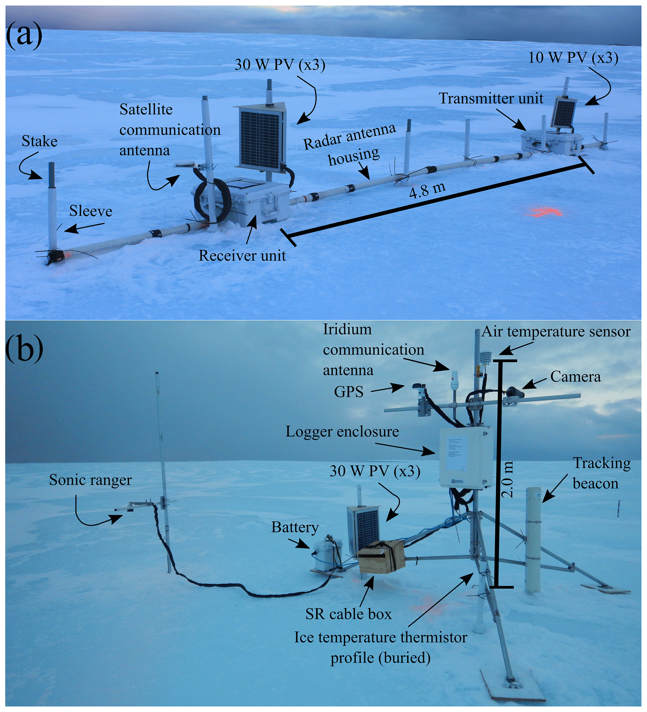
Figure 2Instruments installed on PII-A-1-f on 20 October 2015. (a) Stationary ice-penetrating radar (sIPR) components deployed with antennas “in line” and attached to eight sleeves that slid over stake anchors. (b) Automatic weather station components, including a camera that acquired a weekly image of the sIPR and ablation stakes (not shown). The two systems were installed 30 m apart on two small ridges at the location denoted in Fig. 1c. PV is photovoltaic panel; SR is sonic ranger.

Download

Ice thickness was recorded and telemetered daily by the sIPR (Blue System Integration, Ltd.) until 27 September 2016. Full details regarding this system set-up and measurement specifications can be found in S1 and Mingo et al. (2020). The ice thickness was measured at a resolution of 0.67 m, so the observations were linearly interpolated between dates when step changes in thickness were recorded (16 November 2015–18 September 2016). These dates were used to establish “calibration intervals” for the calibration of the forced convection basal ablation described in the following section.

Daily mean surface ablation was calculated from hourly SR50A sonic ranger (CSCC) height-above-surface (snow or ice) measurements. Surface ablation was also calculated from five ablation stakes that were marked with tape every 10 cm and placed between the meteorological station and the sIPR. A weekly image acquired with a Campbell Scientific CC5MPX camera that was controlled by the meteorological station to visually check on the positioning of the sIPR system also captured these ablation stakes. No snow was present on the date when the stakes and instruments were installed, and the average weekly ablation (or accumulation) at these stakes was calculated with ImageJ (v. 10.8.0) software using the markings for scale (Abramoff et al., 2004). Increases in surface height due to the accumulation of snow are presented in this study as negative values. A linear interpolation was applied to estimate daily ablation or accumulation between these observations so that the sIPR, SR50A, and ablation stake data were available over a consistent time span. Basal ablation was calculated by subtracting the interpolated ablation magnitudes derived from the stake data from the ice thickness time series. These values are therefore approximations of daily basal ablation rates, as they were based on values of ice thickness that were linearly interpolated across longer time periods. Finally, the ablation stake data were used instead of the SR50A data because an unrealistic basal ablation time series was derived from the SR50A data. This was likely caused by a difference in surface conditions between the sIPR and SR50A. It was not possible to assess the surface conditions at the SR50A (30 m away from the sIPR), while the surface conditions were confirmed to be similar between the locations of the ablation stakes and the sIPR (10–15 m away) in weekly images.

3.2 Basal ablation model calibration

3.3 Thinning (spatial assessment)

A repeat transect was conducted to assess spatial variation in thickness and thinning and to verify that the sIPR data were representative with respect to other locations across the ice island. An initial thickness profile was collected with a 25 MHz mIPR (Blue System Integration Ltd.) that was towed by snowmobile over an approximately 3 km transect on 8 May 2016. A series of 10 ablation stakes were also installed along the profile route. Thickness data were collected over 2.4 km of the original transect when the same mIPR system was towed on foot on 28 September 2016. Eight of the stakes were also remeasured at this time. Further details of the mIPR system can be found in S1 and Mingo and Flowers (2010).

All mIPR processing was conducted with Radar Tools (release 0.4), a library of Python scripts and tools that was used to standardize, clean, visualize, and process data contained in the raw radar data (S1; Wilson, 2013). This program was also used to select the location of the air and reflected radar waves. Ice thickness was calculated with Eq. (3) (Wilson, 2012):

where H is thickness (m), s is the distance between the transmitting and receiving antennas (m), t is the time (s) between the recording of the air and reflected waves by the receiver, and v_a is the speed of the electromagnetic wave in air (3.0×10⁸ m s⁻¹) travelling between the transmitter and receiver (Wilson, 2012). The speed of the radar wave in ice (v) was set to 1.7×10⁸ m s⁻¹ (Macheret et al., 1993). The ice thickness resolution (±0.5 m) was limited by v and the waveform sampling interval of the mIPR system (Crawford, 2013).

Snow was present on the ice surface when the mIPR transect was conducted in May 2016. An insufficient number of snow depth measurements were recorded to adequately account for the snow depth over the transect area, and it was not possible to distinguish the snow–ice interface in the radargram. Thickness (ice + snow) in May was therefore calculated using a single velocity value, $v=\mathrm{1.7}\times {\mathrm{10}}^{\mathrm{8}}$ m s⁻¹. However, an additional uncertainty was added to the May ice thickness to account for the possible presence of snow. This uncertainty was based on the mean snow depth (36 cm) recorded at nine locations along the mIPR transect and the amount of time a radar wave would travel through this layer given that $v=\mathrm{2.0}\times {\mathrm{10}}^{\mathrm{8}}$ m s⁻¹ for snow (Haas and Druckenmiller, 2009). The errors associated with the resolution of the mIPR system and the average snow depth estimate were summed to determine the average amount that the ice thickness, as measured in May, could be overestimated by (0.8 m). Uncertainty in thickness change calculations was determined by propagating the uncertainties in ice thickness resulting from the resolution of the mIPR system and the presence of snow.

The magnitude of thinning that occurred between May and September 2016 was calculated between the closest pairs of mIPR traces recorded during each field visit. To improve positional accuracy, the locations recorded by the mIPR onboard GPS were replaced with those recorded by a HiPer V dual-frequency GPS (Topcon Corp.) after precise point positioning (PPP) processing (Natural Resources Canada, 2016). The September transect was adjusted relative to the orientation of PII-A-1-f in May by matching mIPR traces known to be collected at the same location (i.e. the ablation stakes) on the ice island to correct for a small amount of movement by the ice island between the two field visits. Since it was not possible to retrace the transect exactly due to changes in topography between field visits, the thickness measurements that were compared between May and September were offset by varying distances (metres to tens of metres). Using Eq. (4), we derived an index of comparability for these measurements from the percentage of overlap between the radar footprints at the ice–water interface. The radii (r) of these footprints depend on the centre wavelength of the 25 MHz antenna (λ=6.8 m), relative permittivity of ice (K; 3), and H (Leucci et al., 2003),

The positions of thickness change measurements were categorized as ≥50 % overlap, ≥30 % overlap, <30 % overlap, and no overlap.

3.4 Surface extent reduction and contributions to deterioration

The areal extent of PII-A-1-f was monitored with seven RADARSAT-2 FQ SAR scenes to determine the relative importance of surface and basal ablation to the total deterioration of the ice island. The SAR scenes were acquired between 1 November 2015 and 23 September 2017, and the image processing and areal extent digitization details are included in S2. We quantified and compared the contributions of basal ablation, surface ablation, and areal reduction processes (e.g. fracture, forced and buoyant convection, wave erosion, and calving) to the overall deterioration of PII-A-1-f over the temporal-extent sIPR data collection. We also estimated the contribution of surface and basal ablation to total deterioration over the longer temporal extent in which RADARSAT-2 FQ images were acquired. For this estimation, a cubic spline was applied to fill missing cumulative ablation values between 24 September 2016 and 21 October 2016, and it was assumed that the same surface and basal ablation magnitudes that occurred in the first year of observation also occurred between October 2016 and September 2017.

4.1 Thinning (temporal assessment) and environmental conditions

PII-A-1-f decreased in thickness by 4.7±1.4 m over the 11 months that sIPR data were collected and by 4.0±1.4 m during the 10 months that basal ablation was estimated and used for the basal ablation model calibration (Fig. 3a; Table 1). The latter can be divided into three periods related to surface ablation magnitudes as per the ablation stake data (Fig. 3b; Table 1). These are referred to as “ablation periods” in the remainder of the text. Minimal surface ablation was observed over ablation period 1 (November to mid-December 2015). No surface ablation occurred during period 2, which distinguishes it from ablation periods 1 and 3. Therefore, basal ablation was the sole contributor to thinning during ablation period 2, when the mean daily thinning rate was 0.9 cm d⁻¹ (mid-December 2015 to mid-July 2016). The thinning rate tripled during ablation period 3, which spanned from mid-July to September 2016, due to the onset of continuous surface ablation in mid-July. Ninety-eight percent of the recorded surface ablation occurred in this period, when T_a was consistently >0 ^∘C. T_a was >0 ^∘C for 15 % of the second ablation period; however, this contributed to melting the snow that had accumulated on the ice surface instead of ice ablation (Fig. 3b; Table 1).

Table 1Ablation and total thinning magnitudes and rates per ablation period. Air temperature (T_a) data for each period are also included. Inconsistencies exist between the summed ablation and thinning magnitudes or between the ratios of surface: basal ablation magnitudes versus rates are due to rounding. M_s and M_b (in italic font) represent daily surface and basal ablation rates, respectively.

Download Print Version | Download XLSX

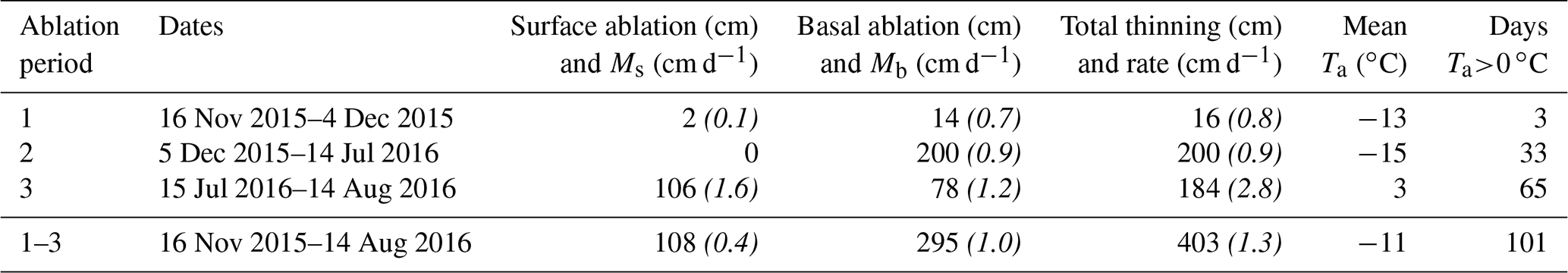
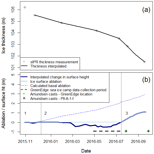
Figure 3Ablation and thickness change. (a) Thickness change of PII-A-1-f as measured by the stationary ice-penetrating radar (sIPR; grey dots) and interpolated between thickness measurements (black line). The first thickness observation was not included in the interpolation due to uncertainty imposed by sIPR measurement resolution. (b) Surface and basal ablation as well as the change in surface height (ht) relative to the start of sIPR data collection. The latter, represented by the thick blue line, includes ice ablation (positive values) as well as snow accumulation (negative values). Basal ablation is calculated with the linearly interpolated thickness values in (a) and should be taken as an estimate of daily magnitudes. The vertical lines denote three surface ablation periods described in Table 1. The timing of CTD profiling by the CCGS Amundsen and the time span associated with oceanographic data collection at the GreenEdge sea ice camp are also denoted.

Download

The mean daily basal melt rate (M_b) between November 2015 and September 2016 was almost 3 times greater than the mean rate of daily surface ablation (M_s; cm d⁻¹). However, this ratio varied between ablation periods. For example, the mean M_b was 7 times greater than the mean M_s during ablation period 1, when only 2 cm of surface ablation was observed. In contrast, the mean M_s was approximately 50 % greater than the mean M_b over ablation period 3, when over 1 m of surface ablation was observed over the 2-month duration (Fig. 3b; Table 1). The mean M_b increased between successive ablation periods (Table 1), and the increase in daily mean M_b from 0.9 to 1.2 cm d⁻¹ between periods 2 and 3 coincides with an increase in CMEMS temperature and velocity. The mean M_b increased between successive ablation periods (Table 1), and the increase in daily mean M_b from 0.9 to 1.2 cm d⁻¹ between periods 2 and 3 coincides with an increase in CMEMS temperature and velocity.

4.2 Basal ablation model calibration

4.2.1 Oceanographic data comparisons

Figure 4 shows the CMEMS Θ, S_A, and u for the duration that PII-A-1-f basal ablation was derived. The mean Θ and S_A of measurements from CTD casts acquired in the vicinity of PII-A-1-f or the GreenEdge sea ice camp are plotted alongside the model data in Fig. 4a and b. These data are associated with the depth interval of the model data that the keel of the ice island fell within for the duration of the data collection. The mean u in this depth interval, as measured by the ADCP moored near to the GreenEdge sea ice camp location, is included in Fig. 4c. The data collected at the GreenEdge sea ice camp (Θ and S_A) and at the nearby moored ADCP (u) provide the longest in situ time series of oceanographic conditions and were used to assess if these variables were consistently over- or underestimated in the CMEMS data.

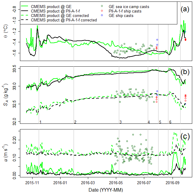
Figure 4Oceanographic data collected or modelled over the time span that PII-A-1-f basal ablation rates were derived. CMEMS product data for the grid cells in which PII-A-1-f (solid black lines) and the GreenEdge sea ice camp (solid green lines) were located: (a) conservative temperature (Θ), (b) absolute salinity (S_A), and (c) velocity (u). As PII-A-1-f was grounded, u is equivalent to the differential velocity between the ice island and the ocean current. Field data collected by the CCGS Amundsen and the GreenEdge project are shown in the respective panels. The CMEMS data, corrected for bias in S_A and u, are shown as dotted lines in (b) and (c), respectively. The vertical lines denote the calibration intervals, numbered in (b), associated with thickness change measurements that were used for the calibration of the forced convection basal melt model. Generated using EU Copernicus Marine Service information.

Download

The means of the absolute daily difference between Θ and S_A at the GreenEdge sea ice camp and the CMEMS data were 0.07 ^∘C and 0.67 g kg⁻¹, respectively. The CMEMS S_A was consistently greater than the in situ data and was therefore corrected by subtracting 0.67 g kg⁻¹ (Fig. 4b, dotted lines). A bias in Θ was not seen, and no correction was applied; however, there was a consistent underestimation of u in the CMEMS data (Fig. 4c). The CMEMS data were corrected by the mean daily difference (0.1 m s⁻¹) between the CMEMS and in situ values of u (Fig. 4c, dotted lines).

CTD profiles collected in the vicinity of PII-A-1-f and the GreenEdge sea ice camp on successive days by the CCGS Amundsen in July and September 2016 were plotted (not shown) to compare the oceanographic conditions at the two sites. In the depth interval of interest, the values of Θ and S_A were reasonably similar and not consistently different between sites. This supported our use of the S_A correction for the CMEMS data that were derived from the difference between the CMEMS data and the longer time series collected at the GreenEdge sea ice camp. This S_A correction was applied to the CMEMS data associated with the location of PII-A-1-f, which was used for the model calibration (Fig. 4b).

The full CMEMS Θ and S_A profiles were also plotted (not shown) against those acquired by the CCGS Amundsen to ensure that the CMEMS data were generally representative of the water column. The CMEMS profiles were reasonable in form, and, in the depth interval of interest, CMEMS consistently overestimated the S_A recorded by the CTD casts acquired by the CCGS Amundsen. The average overestimation was 0.60 g kg⁻¹. This further supports the decision to apply the 0.67 g kg⁻¹ correction to the CMEMS S_A for the forced convection basal ablation model calibration. The CMEMS Θ was both over- and underestimated in the depth interval of interest, which confirms that not applying a correction to this variable was appropriate.

4.2.2 Model calibration and sensitivity analysis

C_i values were calculated with the uncorrected and corrected CMEMS data for each of the six calibration intervals. The range and mean values of C_i calculated with the uncorrected CMEMS data were an order of magnitude larger than those that were theoretically derived by Weeks and Campbell (1973; $\mathrm{6.74}\times {\mathrm{10}}^{-\mathrm{6}}$ m^2∕5 s${}^{-\mathrm{1}/\mathrm{5}}$ ^∘C⁻¹) and White et al. (1980; $\mathrm{1.2}\times {\mathrm{10}}^{-\mathrm{5}}$ m^2∕5 s${}^{-\mathrm{1}/\mathrm{5}}$ ^∘C⁻¹). Due to this, plus the poor representation of uncorrected CMEMS S_A and u, it was decided to further analyze the more reasonable C_i values that were calculated with the corrected CMEMS data. These latter values of C_i are included in Table 2 with the corresponding mean ΔT and u values found with the CMEMS data.

Table 2Calibrated values for C_i for the individual calibration intervals associated with each measured change in ice thickness. The corresponding mean driving temperature (ΔT) and velocity (u) values, found with the CMEMS data, are also provided.

Download Print Version | Download XLSX

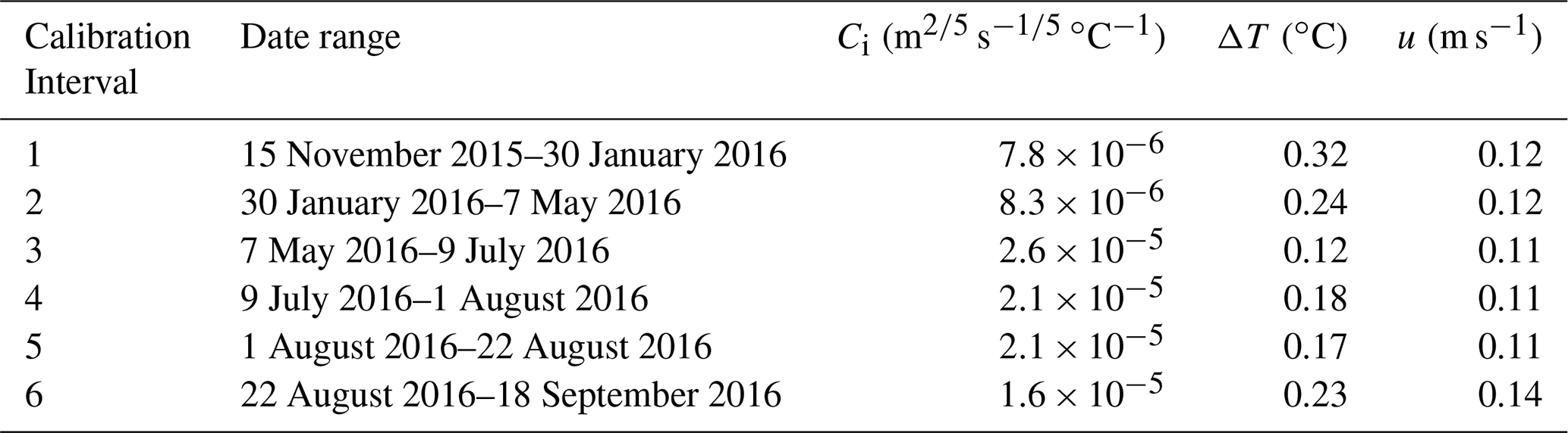
Using these data, the mean C_i value was 1.7×10⁻⁵ m^2∕5 s${}^{-\mathrm{1}/\mathrm{5}}$ ^∘C⁻¹, and values for the individual calibration intervals ranged from $\mathrm{7.8}\times {\mathrm{10}}^{-\mathrm{6}}$ to $\mathrm{2.1}\times {\mathrm{10}}^{-\mathrm{5}}$ m^2∕5 s${}^{-\mathrm{1}/\mathrm{5}}$ ^∘C⁻¹. The greatest values of C_i were associated with calibration intervals 3 through 6. Cumulative basal ablation was over-predicted by 38 % when the forced convection basal ablation model was run with the mean C_i value over the 308 d that basal ablation was calculated. Finally, when calculated with the total basal ablation and total driving force between 15 November 2015 and 18 September 2016, C was calibrated to $\mathrm{1.2}\times {\mathrm{10}}^{-\mathrm{5}}$ m^2∕5 s${}^{-\mathrm{1}/\mathrm{5}}$ ^∘C⁻¹.

Values of u, Θ, and L were not normally distributed. Therefore, the median values of these variables were first assigned during the sensitivity analysis when a given variable was held constant. The calibrated C_i values were found to follow a normal distribution, though the power of this test is low due to the small sample size. For consistency, the median C_i value was also assigned when this parameter was held constant during the sensitivity analysis.

Of the environmental driving variables included in the forced convection basal ablation model, ΔT had the greatest relative range of values over all of the calibration intervals (0.10 to 0.37 ^∘C). A mean increase of 19 % was applied to the ΔT value during the sensitivity analysis, and the same increase in cumulative basal ablation was predicted over the time period that basal ablation was derived with observations. This is due to the linear relationship between ΔT and M_b in Eq. (1) (Table 3).

Table 3Descriptive statistics and sensitivity analysis results. The key driving variables in the forced convection basal ablation model were individually perturbed in eight equal increments based on the variable's range. The sensitivity of the model was assessed as the mean percent increase in predicted cumulative basal ablation following each incremental increase in the value assigned to a given variable. The sensitivity was analyzed over the longer time period (15 November 2015 to 18 September 2016) due to the certainty in the bulk basal ablation.

Download Print Version | Download XLSX

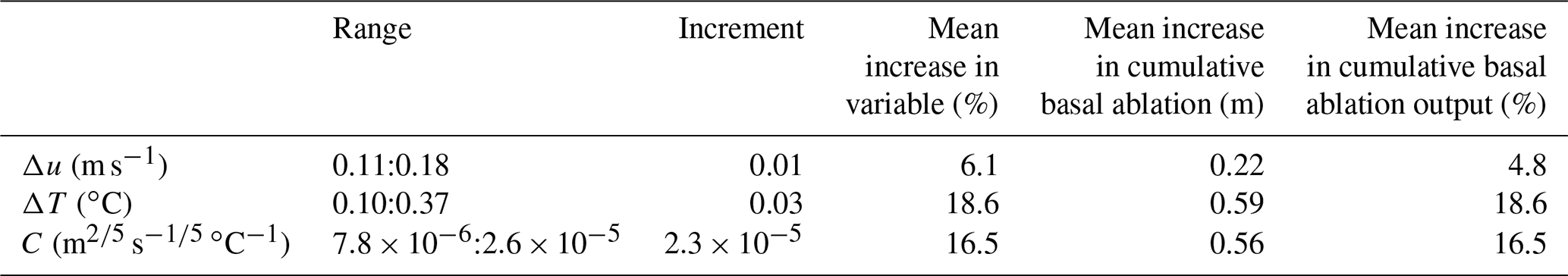
A linear relationship also exists between C and M_b in Eq. (1); however, the range in C_i was more constrained relative to the ΔT data series. For this reason, the cumulative predicted basal ablation only increased by 16.5 % with each incremental change in the value assigned to C during the sensitivity analysis (Table 3). Finally, due to the smaller range of u (0.11 to 0.18 m s⁻¹) and the non-linear relationship between u and M_b in Eq. (1), the relative increment adjustment (6.1 %) and corresponding change (4.8 %) to the predicted cumulative basal ablation over the time period that basal ablation was derived with observations was less than that associated with ΔT or C.

4.3 Thinning (spatial assessment)

The data collected at the main site on PII-A-1-f over 11 months provide unprecedented information regarding the temporal thinning of an ice island. However, these data are representative of a single point on a large ice island. Considering that the rate of surface ablation along the mIPR transect would have been near zero until the snow had melted around 15 July 2016, as determined from the ablation stakes at the sIPR site, the surface would have ablated at a rate of 1.5 cm d⁻¹ after this date. This is slightly less than the rate at the sIPR site over ablation period 3 (1.6 cm d⁻¹; Table 1) and increases the confidence that the surface ablation conditions at the sIPR site were similar to those across the mIPR transect.

The ice island thickness over the mIPR transect ranged from 80.7 to 127.1 [−0.5, +0.8] m in May and 77.3 to 123.7±0.5 m in September 2016 (Fig. 5a). A 50 m long section of relatively thin ice that was approximately 80 m thick was recorded along transect segment AB during both field visits (Fig. 5a); this section was approximately 40 m thinner than adjacent areas. The air and basal wave locations in the mIPR data could not be definitively selected when this thin section was passed during transect segment CD (Fig. 5a). This made it impossible to ascertain thickness at this location; however, a pair of in-line hyperbolae in both the May and September 2016 radargrams support the interpretation that this thinner section ran across both transect segments AB and CD. This section of thin ice is referred to as a “subsurface feature” and corresponds to the location of the linear “surface feature” described in Sect. 2. Together these are referred to as the “paired feature”.

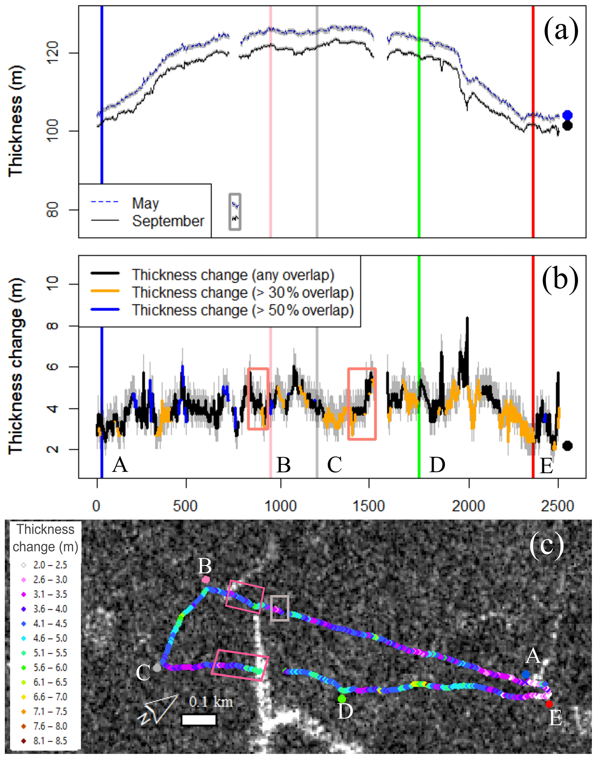
Figure 5Spatial variation in morphology and thinning between May and September 2016. Upper-case letters are used to denote transect segments referred to in the text. (a) Thickness observations collected with mobile ice-penetrating radar. The grey box corresponds with the thin ice section also denoted in (c). (b) Thickness change. The pink boxes indicate thickness change gradients also identified in (c). Thinning data were categorized based on the amount of overlap between the May and September radar footprints. Grey shading in (a) and (b) denotes uncertainty in thickness measurements and thinning amounts, respectively. The larger, single points denote the respective thickness and thinning measured with corresponding data collected by the sIPR at the main site. (c) Thickness change displayed on a Fine Quad RADARSAT-2 synthetic aperture radar scene acquired on 28 September 2016 (shown in greyscale). A surface feature is apparent as a line of high-backscatter (white) pixels starting at the sidewall notch. The geolocation error of the RADARSAT-2 scene was evaluated, and minimal error in the position of the scene was observed.

The magnitude of thinning (3 to 4 m) observed over this thin section present along transect segment AB (shown in the grey boxes in Fig. 5) was in the low to middle range of the thinning observed along the entire transect. However, the general gradient in thinning magnitudes leading to the paired feature shows a similar pattern in both transect segments AB and CD (shown in the pink boxes in Fig. 5). Thinning magnitudes of 3 to 4 m increased to 5 to 6 m across a distance of approximately 90 to 150 m, ending at the surface feature and where a gap in the thickness record exists. A fracture that occurred along this paired feature in September 2017 caused the areal extent of the ice island to reduce by approximately 2.7±0.1 km².

4.4 Volume and area loss and contributions to deterioration

The area and volume of PII-A-1-f were 13.2±0.01 km² and 1.4±0.01 km³, respectively, when it was first visited in October 2015. By September 2016, the volume and areal extent decreased by 0.4±0.01 km³ and 3.4±0.1 km², respectively. A fracture event in September 2016 caused approximately 94 % of the areal reduction and 88 % of this volume loss. These values represent the maximum possible reductions caused by the fracture. Other areal reduction processes (e.g. small-scale calving) would also have contributed to areal reduction during the time interval between RADARSAT-2 acquisitions over which the fracture occurred.

The 23-month RADARSAT-2 monitoring period (October 2015 to September 2017) captured a longer period of areal change. During the latter half of this time span (i.e. September 2016 and September 2017), the ice island un-grounded and re-grounded twice in the same vicinity, and the large September 2017 fracture event occurred (Fig. 1e). The ice island volume decreased by 0.6±0.01 km³ over this period, with the vast majority of this volume loss (94 %) being caused by processes that decreased the areal extent of the ice island. The remaining volume was lost to basal and surface ablation, with basal ablation causing 3 times more volume loss than surface ablation. These ablation magnitudes were extrapolated from the on-ice data collection period. Over the entire 2 years that PII-A-1-f was monitored via RADARSAT-2 image acquisition, areal reduction processes reduced the volume of the ice island by approximately 67 %. Combined, surface and basal ablation resulted in an approximate 7 % reduction of the ice island volume, with basal ablation again causing 3 times more loss than surface ablation.

5.1 Basal ablation model calibrations

Two approaches are predominately used to model ice island and iceberg basal ablation (Bouhier et al., 2018). The first is the semi-empirical fluid-dynamics approach that is calibrated in this study; Eq. (1) approximates melt resulting from the bulk energy transfer occurring within the complex boundary conditions that are present at the ice–water interface (Weeks and Campbell, 1973; White et al., 1980). This model has been widely utilized for iceberg and ice island basal ablation modelling in both the Arctic (Ballicater Consulting, 2012; Bigg et al., 1997; Keghouche et al., 2010; Wagner and Eisenman, 2017) and Antarctic (Gladstone et al., 2001; Martin and Adcroft, 2010; Merino et al., 2016). The second approach is based on thermodynamic principles (Bouhier et al., 2018). Holland and Jenkins (1999) and Hellmer and Obers (1989) document a more complex three-equation thermodynamic model for ice shelf basal ablation, which represents both the salt and temperature flux across the ice–ocean interface.

The forced convection basal ablation model is advantageous due to its computational simplicity and the direct incorporation of Δu. In the thermodynamic approach, the values assigned to the turbulent heat and salt exchange parameters must be adjusted for varying values of Δu in iceberg and ice island applications (Jansen et al., 2007). Jansen et al. (2007) provide calibrated values for three stages of drift, each with a unique range of Δu values for an Antarctic ice island, while Eq. (1) in the forced convection model directly incorporates Δu. Equation (2) was developed to account for the plume of relatively cold and fresh iceberg meltwater that has been observed to surround icebergs and inhibit further melt (Foldvik et al., 1980). This meltwater plume will be stripped from the keel as Δu increases, as is the case when an ice island is grounded (Jansen et al., 2007). Therefore, different parameterizations of Eq. (2) are likely required for predicting the basal ablation of drifting versus grounded ice islands, which FitzMaurice et al. (2017) showed to be the case when parameterizing Eq. (1) for the sidewall melt of an iceberg with different scenarios of meltwater plume and relative ocean velocities. It is possible that an adjustment to the melting point of ice (M_p) to account for the influence of the meltwater plume is not necessary under some conditions, and M_p will simply equal the far-field ocean freezing temperature (Θ_f). Determining this will require concerted study of the difference in the basal boundary layer conditions of grounded versus drifting ice islands. The Δu for a drifting iceberg or ice island will be influenced by both ocean and wind currents (Kubat et al., 2005; Lichey and Hellmer, 2001). Observations of Δu for the drifting ice island case are rare but would be useful for this work and for correctly assigning values to this variable in Eq. (1).

This study used a unique dataset of observed ice island thinning as well as in situ and modelled oceanographic conditions to present a calibration of the forced convection basal ablation model. It is noted that the exponents within Eq. (1), which were derived for the flat plate nature of a tabular iceberg or ice island, could also be calibrated. However, these have remained constant in previous iceberg and ice island literature, while the bulk heat transfer coefficient, C, has typically been assigned one of two values that differ by an order of magnitude. Bigg et al. (1997), Bouhier et al. (2018), Martin and Adcroft (2010), Wagner and Eisenman (2017), and Weeks and Campbell (1973) assign a value of $\mathrm{6.74}\times {\mathrm{10}}^{-\mathrm{6}}$ m^2∕5 s${}^{-\mathrm{1}/\mathrm{5}}$ ^∘C⁻¹. However, the confidence interval of the normal distribution of our calibrated C values does not overlap with this theoretically derived value of the bulk heat transfer coefficient. We recommend assigning the C parameter a value of $\mathrm{1.2}\times {\mathrm{10}}^{-\mathrm{5}}$ m^2∕5 s${}^{-\mathrm{1}/\mathrm{5}}$ ^∘C⁻¹ when modelling ice island basal ablation in the future. This value was calculated from the calibration conducted over the full time span that basal ablation data were available and not the individual calibration intervals associated with the measured changes in ice thickness. In addition, the confidence interval of the normal distribution of C_i values found in Table 2 does overlap with this value. The value also matches, remarkably, that which was theoretically derived by White et al. (1980) and was assigned in the ice island deterioration model used by the CIS (Ballicater Consulting, 2012). We believe that it is more appropriate to use this value instead of the mean of the individually calibrated C_i values reported in Table 2 ($\mathrm{1.7}\times {\mathrm{10}}^{-\mathrm{5}}$ m^2∕5 s${}^{-\mathrm{1}/\mathrm{5}}$ ^∘C⁻¹), as we cannot be sure of the alignment between changes in oceanographic conditions, basal melt rates, and C_i values due to the low resolution of data collected by the sIPR. It is noted that Crawford et al. (2018b) assigned a value of $\mathrm{1.3}\times {\mathrm{10}}^{-\mathrm{5}}$ m^2∕5 s${}^{-\mathrm{1}/\mathrm{5}}$ ^∘C⁻¹ to C, supplied by Crawford (2018), when quantifying the distribution of freshwater input from ice island melt through the eastern Canadian Arctic. The use of this previous value would cause very minimal skew in the distribution of freshwater input, slightly overestimating the freshwater input at the higher latitudes in their study region.

The calibration of the bulk heat transfer coefficient (C) is specific to the approach used to assign an ice temperature when deriving the driving temperature, ΔT. This paper follows the approach of Weeks and Campbell (1973), White et al. (1980), Løset (1993a), Kubat et al. (2005), and Ballicater Consulting (2012), empirically estimating the ice interface temperature (Eq. 2) based on work by Josberger (1977). This contrasts with a line of successive papers (e.g. Bigg et al., 1997; Martin and Adcroft, 2010; FitzMaurice et al., 2016; Wagner and Eisenman, 2017) that assign a constant ice temperature (T_ice) of −4 ^∘C based on Løset (1993b). This study reported temperature measurements at ∼50 cm depth of several iceberg sails in the Barents Sea and show that this temperature will be reached within a few metres of the ice–ocean interface using a model (Løset 1993b). Yet another paper assigns $T_{\mathrm{ice}}=-\mathrm{15}$ ^∘C for sidewall melt calculations (FitzMaurice et al., 2017). These discrepancies underscore the need for harmonization on how T_ice is derived or assigned in the context of the forced convection basal ablation model. We recommend that the melting point of ice be assigned to T_ice in future studies that use this model, as it is the actual temperature of the ice–water interface, easy to calculate, and physically meaningful. Our recommendation is also supported by the model comparison and sensitivity study of FitzMaurice and Stern (2018); this work found that the thermodynamic and forced convection models agree when T_ice=M_p and infer that the heat flux into the iceberg interior is small. For the sake of inter-comparison, example calculations using L, S_A, Θ, and u values representative of conditions at PII-A-1-f, the calibrated value of C would decrease by 1 order of magnitude if $T_{\mathrm{ice}}=-\mathrm{4}$ ^∘C. The calibrated C value would then be in line with that derived by Weeks and Campbell (1973). The value of C would decrease by 2 orders of magnitude if −15 ^∘C were assigned to T_ice.

The in situ dataset of oceanographic conditions in the vicinity of PII-A-1-f and the GreenEdge sea ice camp was of paramount importance for validating and correcting the CMEMS data for bias. However, the calibration could be further improved by obtaining a longer time series of oceanographic data in closer proximity to the ice island. In general, there is a paucity of in situ oceanographic data collected in the vicinity of ice islands. Collection of such data will allow for further improved drift and deterioration analyses of icebergs and ice islands. Modifying the sIPR to resolve smaller magnitudes of thickness change is also recommended. This would make it possible to relate these higher-quality thinning measurements to corresponding surface ablation and recorded oceanographic conditions.

5.2 Ablation rates and contributions to overall deterioration

Field measurements of ice island thinning are extremely sparse. Scambos et al. (2008) installed numerous instruments on two Antarctic tabular icebergs while investigating their deterioration processes with field and remote-sensing data. Unfortunately, it was impossible to process thickness measurements collected by a radio-echo sounder installed on one of the icebergs (Scambos et al., 2008). Prior to our study, the spot values reported by Halliday et al. (2012) from a 17 km² ice island drifting in the Labrador Sea were the only known field observations of ice island thinning. The PII-A-1-f thinning dataset greatly improves on this previous work, as the long-term sIPR time series and repeat mIPR transects together produce a comprehensive dataset that allows us to assess the spatial and temporal variations in thinning and ablation. It would be highly beneficial to redeploy the sIPR on a drifting ice island in the future to (1) augment the number of observations of ice island thinning and (2) begin comparing basal ablation occurring to drifting versus grounded ice islands.

The average M_b of 3.4 cm d⁻¹ reported by Halliday et al. (2012) was greater than that observed for PII-A-1-f. Since the basal ablation rate for a drifting ice island should be lower than that of a grounded ice island due to decreased Δu and the potential protection of a meltwater plume, this greater melt rate was likely due to the higher Θ off the coast of Labrador. Elevated ocean temperatures also contributed to the high, 13.5 m month⁻¹ basal ablation rate that Jansen et al. (2007) estimated for the grounded Antarctic ice island “A38-B”. Basal ablation was reported to cause 96 % of the thinning of this ice island that had a surface extent of approximately 7600 km² (Jansen et al., 2007), whereas 73 % of the thinning of PII-A-1-f was a result of this process. We note that, when present, the densification of firn is a factor in the surface ablation of Antarctic tabular icebergs. Scambos et al. (2008) document firn characteristics on two Antarctic tabular icebergs, and a follow-up field study that combines such observations with repeated thickness measurements would be valuable for assessing the contributions of surface and basal processes to Antarctic iceberg thinning.

While basal ablation was responsible for the majority of the thinning of PII-A-1-f, this process caused the ice island volume to reduce by approximately 5 %. However, basal ablation indirectly influences further deterioration by reducing the relative thickness of the ice island and decreasing fracture resistance (Goodman et al., 1980; Jansen et al., 2005). This will happen more quickly if an ice island is grounded, as basal ablation could increase by a factor of 2 after an ice island stops drifting freely (Jansen et al., 2007). Future research, including finite-element modelling (e.g. Sazidy et al., 2019), is warranted to assess if and how thinning contributed to the September 2017 calving event. This fracture occurred along the paired feature that was substantially thinner than adjacent ice surfaces and which emanated from the root of the sidewall notch. We also recommend that further research be conducted into the relationship between the presence of the paired feature, the propagation of the sidewall notches before and during the time that PII-A-1-f was grounded in southern Baffin Bay, and the ultimate September 2017 fracture. The enlargement of sidewall notches, similarly to cusped deterioration patterns observed by Ballicater Consulting (2012), is a recurring deterioration mechanism that is not considered in deterioration studies or models at this point in time.