2.1 Ice sheet model

We use the 1D isothermal flow line model with higher-order momentum balance described in Brinkerhoff et al. (2017). The momentum conservation equations are simplified using the Blatter–Pattyn approximation, assuming hydrostatic pressure and negligible vertical resistive stresses (Blatter, 1995; Pattyn, 2003). Default parameter values used in this work are specified in Table 1.

We adopt a linear sliding law of the form

where τ_b is basal shear stress, β² is a constant basal traction parameter, N is effective pressure, and u_b is sliding speed. Based on borehole water pressure measurements in Wright et al. (2016), basal water pressure P_w is assumed to be a fixed fraction P_frac=0.85 of ice overburden pressure P₀. Effective pressure is therefore given by

The basal traction parameter β² is tuned to minimize the misfit between modeled and observed surface velocities from Mouginot et al. (2017) for present-day Isunnguata Sermia values.

2.2 Flow line selection and moraine age constraints

To define the path followed by ice, we assume that flow follows the modern surface velocity field inland of the present-day margin. In ice-free regions, the direction of ice flow is inferred from bedrock topography (Fig. 1). Since the direction of ice flow is unknown and time varying, we cannot directly quantify the uncertainty introduced by errors in flow line selection. To account for some of this uncertainty, we perform inversions on two plausible adjacent paleo-flow lines in the Kangerlussuaq area.

The rate of Holocene retreat on each flow line is estimated using constraints on ice sheet terminus position from (Young et al., 2020) (Fig. 1). Terminus position data in Young et al. (2020) indicate that in the early Holocene (11.6 ka), the ice sheet margin was tens of kilometers inland of the present-day coastline. Although the moraine patterns are spatially complex, generally speaking there was a period of moderate retreat (∼10 km on the northern flow line and ∼30 km on the southern flow line) from 11.6 to 10.3 ka, followed by rapid retreat (∼100 km on both flow lines) from 10.3 to 8.1 ka. By 8.1 ka, the margin position was within 20 km of its present position on both flow lines (Fig. 5). The modern terminus position provides one additional constraint. Moraine ages have uncertainties of up to ±400 years.

For modern bedrock geometry along the flow lines, we use BedMachine v3 (Morlighem et al., 2017). Isostatic uplift and relative sea level changes are accounted for using a glacial isostatic adjustment model (Caron et al., 2018). This model, combined with the retreat chronology in Young et al. (2020), indicates that ice remained grounded on both the northern and southern flow lines from 11.6 ka onward.

2.3 Positive degree day model

Surface mass balance is estimated using a positive degree day (PDD) model (Johannesson et al., 1995). Annual surface mass balance is constructed in the PDD model using estimates of average monthly precipitation and temperature. Inputs into the PDD model include the unknown ice surface elevation S, modern monthly temperature T_m and precipitation P_m along the flow lines, as well as the seasonal temperature anomaly ΔT. As in Cuzzone et al. (2019), modern temperature and precipitation are computed as 30-year averages from 1980 to 2010 using the method of Box (2013).

To assess the sensitivity of modeled retreat history to temperature, we perform experiments using temperature reconstructions from both Buizert et al. (2018) and Dahl-Jensen et al. (1998). For the spatially explicit Buizert et al. (2018) reconstruction, monthly temperature anomalies are computed as averages along the flow lines. In contrast, Dahl-Jensen et al. (1998) reconstruct temperature only at the GRIP and Dye-3 borehole locations (Fig. 1). Since a full Holocene reconstruction is unavailable at the Dye-3 borehole site, which is closer to Kangerlussuaq, we use the temperature reconstruction at GRIP. The HTM is roughly 0.3 ^∘C warmer and 1500 years later in Dahl-Jensen et al. (1998) than in Buizert et al. (2018) (Fig. 6).

A limitation of the Dahl-Jensen et al. (1998) reconstruction is that it does not resolve seasonal temperatures. To address this, we calculate the difference between monthly and mean annual temperatures in Buizert et al. (2018) and apply those offsets to the mean annual temperature at GRIP from Dahl-Jensen et al. (1998).

Surface temperature T is computed monthly as

where S_m is the modern surface elevation and α= 5^∘C km⁻¹ is the lapse rate (Abe-Ouchi et al., 2007). Following Ritz et al. (2001) and Cuzzone et al. (2019), precipitation P along the flow line is estimated based on the Clausius–Clapeyron relation. In particular, precipitation is estimated by

The term P_T accounts for changes in precipitation solely due to changes in temperature. Here λ_P=0.07, which results in a 7 % increase in precipitation for every 1 ^∘C increase in temperature above modern (Abe-Ouchi et al., 2007; Ritz et al., 2001).

The term P_T does not capture the effects of many unknown climate factors that may have caused dynamic regional changes in Holocene precipitation. Therefore, we introduce a precipitation anomaly term ΔP, analogous to the temperature anomaly ΔT. This time-dependent function, which has units of meters water equivalent per annum (m w.e. a⁻¹), is used to adjust precipitation uniformly across a flow line in order to reduce mismatch between modeled and observed terminus positions. Unlike ΔT, which can be inferred from ice cores, ΔP will be used as a control variable to be determined using the inverse methods detailed in Sect. 2.5.3. Equations (3) and (4) provide a method of accounting for elevation changes through time and downscaling inputs to match the mesh resolution of the model (∼1 km).

Positive degree days and snowfall are computed month by month based on mean monthly temperature and precipitation (Johannesson et al., 1995). Snow is melted first at a rate of $\mathrm{5}\times {\mathrm{10}}^{-\mathrm{3}}$ m w.e. ^∘ d⁻¹ followed by ice at a rate of $\mathrm{8}\times {\mathrm{10}}^{-\mathrm{3}}$ m w.e. ^∘ d⁻¹. Snow melt is initially supposed to refreeze in the snowpack as superimposed ice. Runoff begins when the superimposed ice reaches a given fraction (60 %) of the snow cover (Reeh, 1991). A listing of ice flow and PDD model parameters is provided in Table 1, and all data sets used in the model are shown in Table 2.

2.4 Modeling limitations

A limitation of our modeling approach is that we do not account for potential ice dynamical effects caused by changes in surface runoff or subglacial hydrology. Modeling melt water runoff would be difficult in a flow line model due to flux of melt water in and out of the path of ice flow. Another limitation is that our model is isothermal. Unless ice temperature is treated in a vertically averaged sense, resolving temperature would require a 2D mesh, which would considerably increase the computational cost of the model. We consider the consequences of this simplification in Sect. 3.3, where we test sensitivity to the ice hardness parameter.

The PDD scheme outlined in Sect. 2.3 does not account for changes in surface mass balance due to orographic forcing or other complex interactions between the ice sheet and climate system that could be captured by coupling the ice sheet model to an Earth system model (Bahadory and Tarasov, 2018). Since our emphasis is on estimating precipitation and surface mass balance using an inverse modeling approach, we believe the computational cost of such an approach outweighs the benefits. Uncertainties related to feedbacks between ice dynamics and climate are assessed via extensive sensitivity testing (Sect. 3.3).

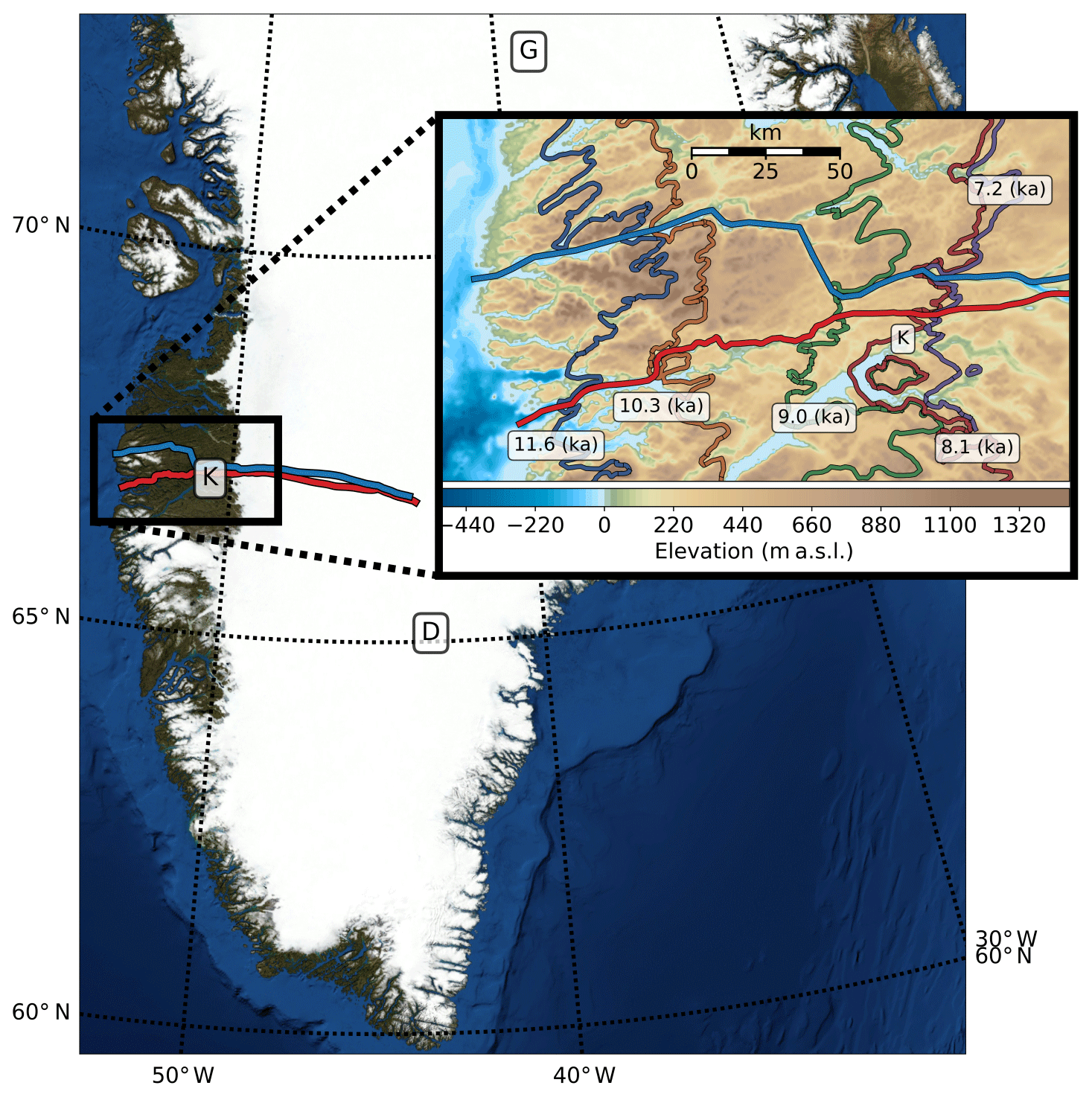
Figure 1K marks the position of Kangerlussuaq, while D and G mark the locations of the Dye-3 and GISP2 boreholes, respectively. Northern and southern paleo-flow lines are shown as blue and red lines running left to right. The inset shows a detailed view of the modeled region. Modern bedrock elevation is expressed in meters above sea level. Historical moraines dating from 11.6 to 7.2 ka are indicated by labeled lines.

Table 1Summary of primary model parameters used in this work. Default values are provided where applicable.

Download Print Version | Download XLSX

2.5 Data assimilation approach

In order to assess the initial mismatch between modeled and observed retreat histories, we perform a reference experiment with ΔP=0 and ΔT estimates from both Buizert et al. (2018) and Dahl-Jensen et al. (1998). To improve the fit to observations, we assimilate terminus position data to obtain improved estimates of Holocene precipitation anomalies. Previous modeling studies indicate that Holocene retreat in land-terminating sectors of the GrIS were dominated by surface mass balance rather than ice dynamics (Cuzzone et al., 2019; Lecavalier et al., 2014). Uncertainty in Holocene climate, and consequently surface mass balance, is therefore likely the primary cause of discrepancies between modeled and observed terminus positions.

In principle, ΔP, ΔT, or both could be tuned to improve the fit between modeled and observed terminus positions. We focus on precipitation because it is more poorly constrained than temperature. In the upcoming sections, we introduce a framework for time-dependent data assimilation based on the unscented transform (UT). Sections 2.5.1–2.5.2 outline the basic tenets of the UT. Sections 2.5.3–2.5.7 outline how the UT can be applied to estimate precipitation anomalies.

2.5.1 Overview of the unscented transform

In what follows, the notation x∼𝒩(x₀, P_x) means that x is a normally distributed random variable with mean vector x₀ and covariance matrix P_x. Suppose that $\mathit{x}\sim \mathcal{N}({\mathit{x}}_{\mathrm{0}},{\mathbf{P}}_x$), and $\mathcal{F}:{\mathbb{R}}^{\mathrm{n}}\to {\mathbb{R}}^{\mathrm{m}}$ is a nonlinear function. We would like to estimate the distribution of the non-Gaussian random variable

$$\begin{array}{}\text{(5)}& \mathit{y}=\mathcal{F}\left(\mathit{x}\right)+\mathit{ϵ},\end{array}$$

where $\mathit{ϵ}\sim \mathcal{N}(\mathbf{0},\mathbf{R}$) is the measurement noise.

In general, the non-Gaussian probability distribution for y can be approximated using Markov chain Monte Carlo (MCMC) methods such as the Metropolis–Hastings algorithm (Chib and Greenberg, 1995). However, if the nonlinear function is time-consuming to compute, generating thousands of MCMC samples is often intractable. As a computationally efficient alternative to MCMC methods, Julier and Uhlmann (1997) introduced a method for approximating the mean and covariance of y called the unscented transform (UT) ¹.

The term unscented transform has been applied somewhat broadly to a family of methods that approximate the statistical moments of a non-Gaussian random variable using a small, deterministic set of sample points called sigma points. It is known primarily in the context of the unscented Kalman filter. However, the UT can be applied more generally as an alternative to traditional MCMC methods. Sigma points and weight sets are designed to accurately estimate moments of a transformed random variable using a minimal number of function evaluations.

A set of vectors, called sigma points, are chosen with the same weighted sample mean and weighted covariance structure as x. There are many algorithms for generating sigma points sets with different numbers of points and orders of accuracy. A commonly used set of 2n+1 sigma points is given by

$$\begin{array}{}\text{(6)}& {\mathit{\chi }}_i=\left\{\begin{array}{ll}{\mathit{x}}_{\mathrm{0}}& i=\mathrm{0}\\ {\mathit{x}}_{\mathrm{0}}-\sqrt{n+\mathit{\kappa }}[\sqrt{{\mathbf{P}}_x}{]}_i& i=\mathrm{1},\mathrm{\dots },n\\ {\mathit{x}}_{\mathrm{0}}+\sqrt{n+\mathit{\kappa }}[\sqrt{{\mathbf{P}}_x}{]}_i& i=n+\mathrm{1},\mathrm{\dots },\mathrm{2}n\end{array}\right.,\end{array}$$

with corresponding mean and covariance weights given by

$$\begin{array}{}\text{(7)}& w_i^{\left(\mathrm{m}\right)}=w_i^{\left(\mathrm{c}\right)}=\left\{\begin{array}{ll}\mathit{\kappa }/(n+\mathit{\kappa })& i=\mathrm{0}\\ \mathrm{1}/\mathrm{2}(n+\mathit{\kappa })& \text{otherwise}\end{array}\right..\end{array}$$

The notation ${\left[\sqrt{{\mathbf{P}}_x}\right]}_i$ refers to the ith row of a matrix square root (typically computed by Cholesky factorization) of P_x, and κ is a free parameter controlling the scaling of the sigma points around the mean. Julier and Uhlmann (1997) recommend a default value of $\mathit{\kappa }=\mathrm{3}-n$. However, κ can be fine-tuned to reduce prediction errors for a given problem.

Young et al. (2020)Morlighem et al. (2017)Mouginot et al. (2017)Box (2013)Buizert et al. (2018)Dahl-Jensen et al. (1998)Caron et al. (2018)

Table 2Citations for the primary data sets used in this work.

Download Print Version | Download XLSX

The nonlinear function ℱ is applied to each sigma point to yield a set of transformed points

$$\begin{array}{}\text{(8)}& {\mathcal{Y}}_{\mathit{i}}=\mathcal{F}\left({\mathit{\chi }}_i\right).\end{array}$$

The mean $\stackrel{\mathrm{‾}}{\mathit{y}}$ and covariance matrix P_y of y are then estimated as weighted sums.

$$\begin{array}{}\text{(9)}& \stackrel{\mathrm{‾}}{\mathit{y}}=\sum _{i=\mathrm{0}}^{\mathrm{2}n}{w}_i^{\left(\mathrm{m}\right)}{\mathcal{Y}}_{\mathit{i}}\end{array}$$

$$\begin{array}{}\text{(10)}& {\mathbf{P}}_y=\sum _{i=\mathrm{0}}^{\mathrm{2}n}{w}_i^{\left(\mathrm{c}\right)}({\mathcal{Y}}_{\mathit{i}}-\stackrel{\mathrm{‾}}{\mathit{y}})({\mathcal{Y}}_{\mathit{i}}-\stackrel{\mathrm{‾}}{\mathit{y}}{)}^T+\mathbf{R}\end{array}$$

A visual example of this algorithm is shown in Fig. 2.

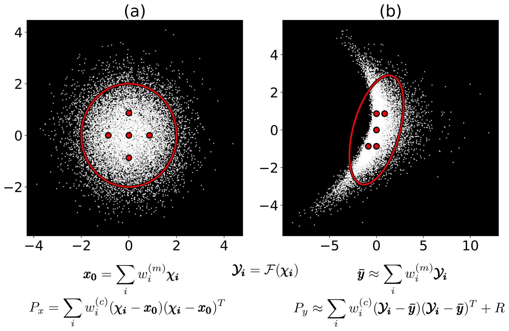
Figure 2(a) White points are samples from a 2D Gaussian distribution $\mathit{x}\sim \mathcal{N}(\mathbf{0},I$). The red ellipse represents the covariance of the distribution, while red points are sigma points χ_i used for the unscented transform (UT). (b) White points are samples from the transformed, non-Gaussian distribution for $\mathit{y}=\mathcal{F}\left(\mathit{x}\right)+\mathit{ϵ}$ with $\mathit{ϵ}\sim \mathcal{N}(\mathbf{0},\mathbf{R}$). Red points are transformed sigma points 𝓨_i=ℱ(χ_i). UT approximations of the mean $\stackrel{\mathrm{‾}}{\mathit{y}}$ and covariance P_y of y are estimated via weighted sums of transformed sigma points.

Download

2.5.4 Gaussian process prior for regularization

We adopt a Gaussian process prior (Rasmussen, 2004) to control the temporal smoothness of ΔP. A Gaussian process can be thought of as a distribution over functions. That is, random samples from a Gaussian process are functions rather than individual points or vectors. A collection of random variables $\mathit{\left\{}f\right(t):t\in \mathcal{T}\mathit{\}}$ is said to be drawn from a Gaussian process with mean function m(⋅) and covariance function $k(\cdot ,\cdot$) if, for any finite set of elements $t_{\mathrm{1}},\mathrm{\dots },t_n\in \mathcal{T}$, the random variables $f\left(t_{\mathrm{1}}\right),\mathrm{\dots },f(t_n$) have the distribution

$$\begin{array}{}\text{(24)}& \mathit{f}\sim \mathcal{N}\left(\mathit{m},\mathbf{K}\right),\end{array}$$

with

$$\begin{array}{}\text{(25)}& \mathit{f}=\left[f\right(t_{\mathrm{1}}),f(t_{\mathrm{2}}),\mathrm{\dots },f(t_n){]}^T,\end{array}$$

$$\begin{array}{}\text{(26)}& \mathit{m}=\left[m\right(t_{\mathrm{1}}),m(t_{\mathrm{2}}),\mathrm{\dots },m(t_n){]}^T,\end{array}$$

and

$$\begin{array}{}\text{(27)}& \mathbf{K}=\left[\begin{array}{ccc}k(t_{\mathrm{1}},t_{\mathrm{1}})& \mathrm{\dots }& k(t_{\mathrm{1}},t_n)\\ \mathrm{⋮}& \mathrm{\ddots }& \mathrm{⋮}\\ k(t_n,t_{\mathrm{1}})& \mathrm{\dots }& k(t_n,t_n)\end{array}\right].\end{array}$$

The set 𝒯 is called the index set, and specifies the domain of the Gaussian process. Here, the index set represents points in time.

The prior distribution for Δp has mean vector Δp₀ and covariance matrix P₀=K of the form shown in Eq. (27). We use a squared exponential covariance function

$$\begin{array}{}\text{(28)}& k(t,t^{\prime })={\mathit{\sigma }}_P^{\mathrm{2}}\exp \left({\displaystyle \frac{(t-t^{\prime }{)}^{\mathrm{2}}}{\mathrm{2}{\mathit{\tau }}^{\mathrm{2}}}}\right),\end{array}$$

where σ² is a scaling constant and τ is a characteristic timescale. Variables Δp_i and Δp_k are more highly correlated the closer they are in time. In effect, this acts as a form of temporal regularization, in which smooth precipitation history functions are preferred over less smooth ones. We discuss the choice of the mean Δp₀ in Sect. 3.2.

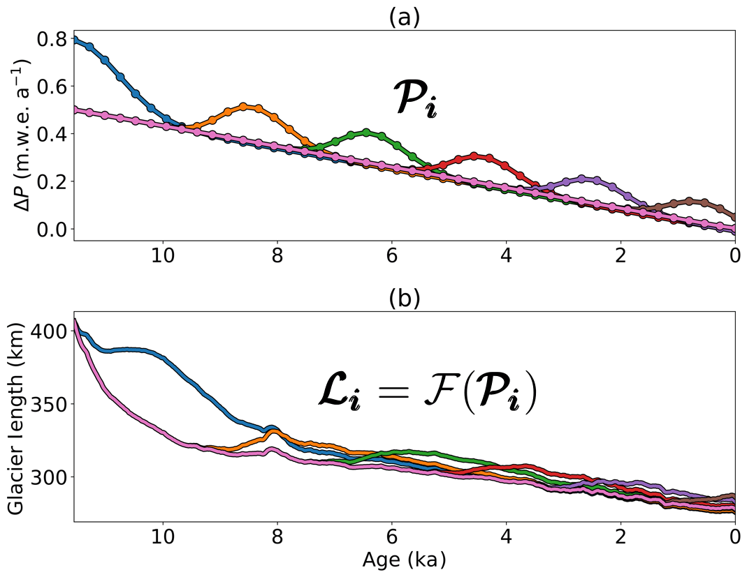
Figure 3(a) A subset of 6 out of a total of 45 Menegaz et al. (2011) sigma points 𝓟_i representing different precipitation anomaly histories. (b) Six corresponding glacier length histories 𝓛_i or transformed sigma points obtained by inputting the sigma points 𝓟_i into the ice dynamics model ℱ.

Download

2.5.6 Iterative optimization procedure

Optimizations are conducted in multiple passes. In the first pass, the measurement covariance matrix R is multiplied by a factor of 0.25 so that the measurements are initially weighted more than the prior. This produces a reasonable fit to the data, even given a poor initial estimate of ΔP. The optimal precipitation anomaly from a given iteration is used as the prior mean in the next iteration. We use the same prior covariance matrix P₀ for regularization in each iteration. After two to three iterations, modeled and observed terminus positions match within measurement uncertainty (Sect. 3). In our experience, the results of iteration are not dependent on the choice of prior mean in the first iteration, but we find that convergence can be improved by choosing a sensible initial guess, as in Sect. 3.2.

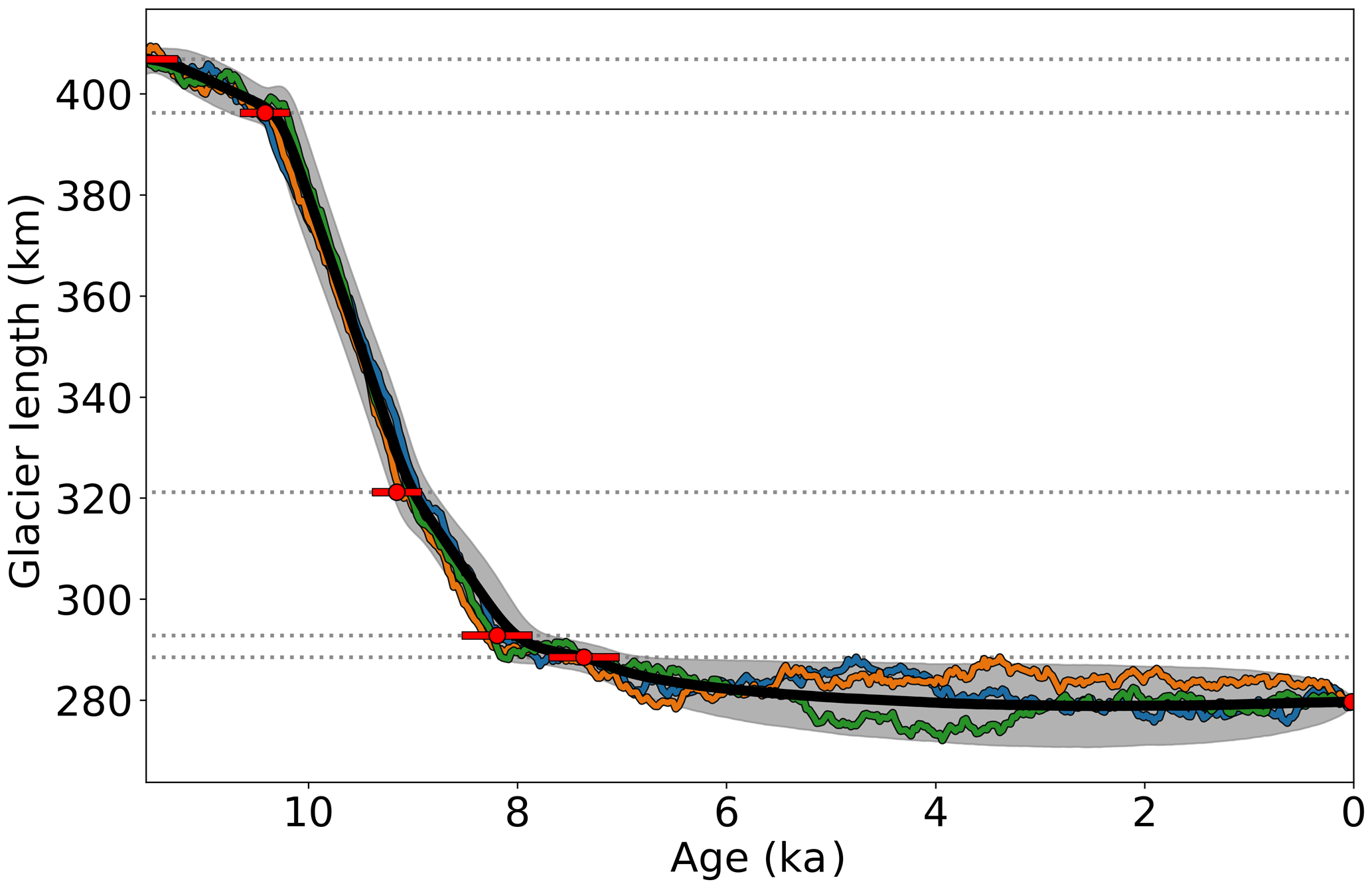
Figure 4The measurement mean ℓ₀ (solid black line) and 95 % confidence bands (gray shaded region) for the northern flow line are estimated by generating random retreat histories with the same mean moraine formation ages and variances as the observations. The green, blue, and orange lines represent four random plausible retreat histories. Red dots denote the estimated mean moraine formation ages, while red lines show 95 % confidence intervals.

Download

2.6 Model initialization

Model runs are initialized by tuning the precipitation anomaly to obtain a steady state at 12.6 ka, with a margin position 5 km beyond the 11.6 ka moraine. We invert for a precipitation anomaly time series that forces a retreat of 5 km over 1000 years to obtain an initial ice sheet configuration with the correct terminus position at 11.6 ka (Fig. 5). This initialization procedure is intended to ease the ice sheet out of steady state in order to avoid strong transient effects at the beginning of model runs.

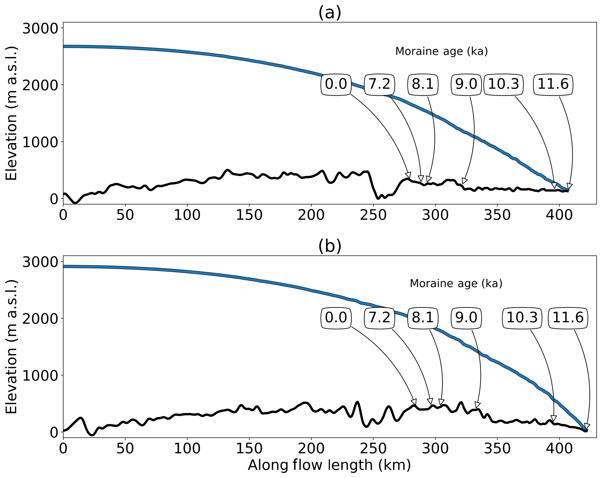
Figure 5Initial ice sheet configurations for the northern (a) and southern (b) paleo-flow lines. Solid black and blue lines represent the bedrock elevation and ice surface, respectively. Moraine positions are indicated by arrows with associated ages expressed in thousands of years before present.

Download

3.1 Reference experiment

To assess the initial misfit between modeled and observed Holocene retreat, the model is forced with ΔT reconstructions from Buizert et al. (2018) and Dahl-Jensen et al. (1998) and a zero precipitation anomaly. Precipitation is scaled with temperature according to Eq. (4), neglecting possible influences from changing Arctic sea ice cover, atmospheric circulation, or other unknown climate factors. Modeled ice retreat is far more rapid than observed on both flow lines (Fig. 8). Colder temperatures during the early Holocene (Fig. 8a) lead to a somewhat more plausible retreat history using the Dahl-Jensen et al. (1998) temperature forcing versus the Buizert et al. (2018) forcing. However, by 8 ka, ice has retreated inland of the present-day margin in both reconstructions.

3.2 Precipitation anomaly inversions

We estimate precipitation anomalies on the northern and southern flow lines using both the Buizert et al. (2018) and Dahl-Jensen et al. (1998) temperature reconstructions. Given the rapid retreat in the reference experiment, we expect that a positive precipitation anomaly will be required to match observed terminus positions in the early Holocene. Therefore, in the first round of optimization, we assume a prior mean of the form

where $\widehat{\mathit{\tau }}$ is a rescaled time variable that increases from zero at 11.6 ka to one at 0 ka. The results of the iterative optimization procedure are insensitive to the prior mean selected in the first iteration. Using a sigma point scaling parameter w₀=0.5 for the Menegaz et al. (2011) sigma point set ensures that a wide region around the mean is explored in each iteration.

Positive precipitation anomalies are predicted throughout most of the Holocene for both temperature reconstructions (Fig. 6). While differences between the northern and southern flow lines are relatively minor, there are significant differences in precipitation between the Buizert et al. (2018) and Dahl-Jensen et al. (1998) inversions. In the Buizert et al. (2018) inversion, the largest precipitation anomalies (up to 1 m w.e. a⁻¹) occur during the early Holocene. Precipitation remains relatively high during the HTM (10–6 ka) but dips before the 8.2 ka cold event. For the Dahl-Jensen et al. (1998) inversion, ΔP is relatively low during the early Holocene but increases during the HTM (8.5–3 ka). Unlike the Buizert et al. (2018) inversion, there is an evident trend between HTM warming and increased snowfall (Fig. 9).

Forcing the model with mean estimated precipitation anomalies yields plausible retreat histories on both flow lines. Modeled and observed retreat chronologies match within uncertainty (Fig. 8). A significant fraction of Holocene precipitation (typically >90 %) falls as snow. Hence, a positive precipitation anomaly can be interpreted directly as additional snowfall and snow accumulation. Average HTM snowfall is around 35 % higher than modern in both temperature reconstructions (Fig. 9). However, overall trends in Holocene snowfall differ between reconstructions.

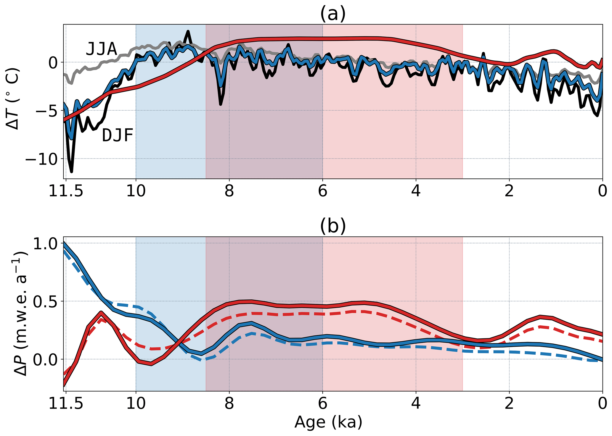
Figure 6(a) Buizert et al. (2018) and Dahl-Jensen et al. (1998) mean annual temperature anomalies are shown as blue and red lines, respectively. Gray and black lines, respectively, show average December, January, February (DJF) and June, July, August (JJA) temperature anomalies for the Buizert et al. (2018) reconstruction. Shaded blue and pink regions demarcate the extent of the HTM for the Buizert et al. (2018) and Dahl-Jensen et al. (1998) reconstructions. (b) Estimated precipitation anomaly histories for the Buizert et al. (2018) and Dahl-Jensen et al. (1998) inversions are shown by blue and red lines, respectively. Solid lines show estimates for the northern flow line, while dashed lines are for the southern flow line.

Download

Figure 7Average precipitation (both solid and liquid) on the northern flow line from the Buizert et al. (2018) reconstruction (black line), which is based on the TraCE-21ka coupled ocean–atmosphere general circulation model of the last deglaciation versus estimated precipitation derived in this work based on reconciling the modeled and observed retreat chronologies (blue line).

Download

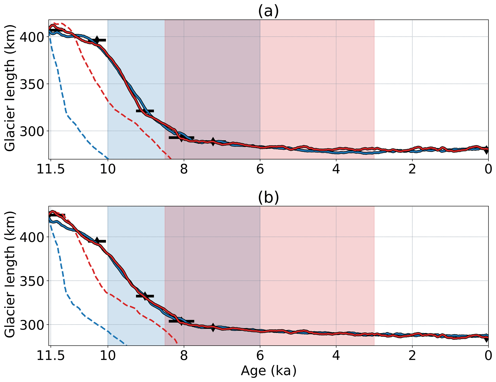
Figure 8Modeled retreat histories for the northern (a) and southern (b) flow lines using a variety of ΔT and ΔP forcings. Blue and red lines show modeled retreat using Buizert et al. (2018) and Dahl-Jensen et al. (1998) temperature forcings, respectively. Dashed lines show the results of forcing the model with ΔP=0, while solid lines show the results of using optimal estimated precipitation anomalies. Black diamonds and bars show reconstructed terminus positions, along with 95 % confidence intervals. Shaded blue and pink regions demarcate the extent of the HTM for the Buizert et al. (2018) and Dahl-Jensen et al. (1998) reconstructions, respectively.

Download

Figure 9HTM snowfall averaged across the northern and southern flow lines for the Buizert et al. (2018) (solid blue line) and Dahl-Jensen et al. (1998) (solid red line) inversions. Shaded blue and pink regions demarcate the extent of the HTM for the Buizert et al. (2018) and Dahl-Jensen et al. (1998) reconstructions, respectively. Dashed lines show pre-HTM, HTM, and post-HTM average snowfall for each inversion.

Download

3.3 Sensitivity testing

We assess the sensitivity of Holocene precipitation anomalies to modeling uncertainties by performing an HTM inversion using the methodology described in Sect. 2.5.7. To obtain accurate uncertainty estimates, we use a fifth-order accurate sigma point set based on Li et al. (2017) (Appendix A), as we find that the second-order Menegaz et al. (2011) set likely underestimates covariance. Inversions are performed on the northern flow line using the Buizert et al. (2018) temperature reconstruction. Model runs are initialized from steady states around at 10.5 ka, 500 years prior to the Buizert et al. (2018) HTM. Prior and posterior parameter values are reported in Table 3.

Table 3Summary of primary model parameters used in this work. Default values are provided where applicable. Prior parameter uncertainties assumed for the sensitivity test are shown in the 2σ column.

Download Print Version | Download XLSX

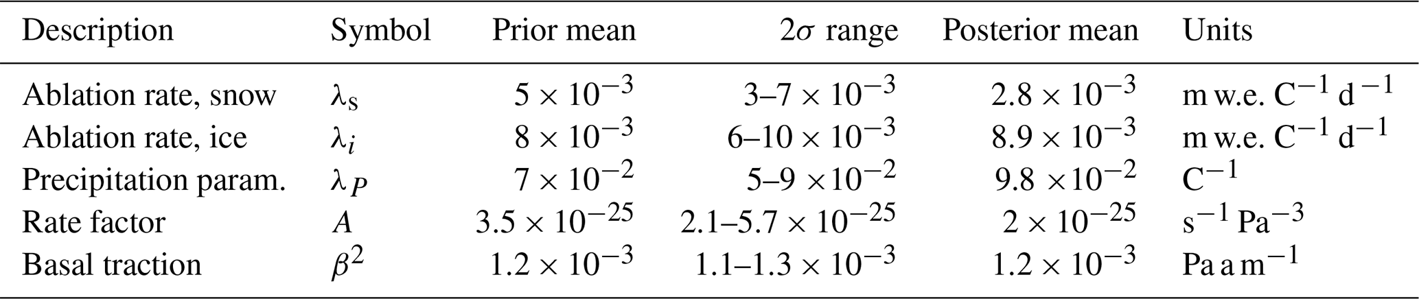
Mean HTM precipitation anomalies are within 2 cm w.e. a⁻¹ of the inversion presented in Sect. 3.2 (Fig. 10). Parameter uncertainties contribute to uncertainty in ΔP. Overall, however, temperature uncertainty is far more significant than uncertainty in model parameters. Differences in model initialization do not significantly impact the results of the inversion. Although sensitivity tests are initialized from steady states at 10.5 ka, while inversions in Sect. 3.2 are initialized from a transient state at 11.6 ka, the mean HTM precipitation anomalies are nearly identical. Estimated posterior parameter values are also similar to the assumed prior values (Table 3).

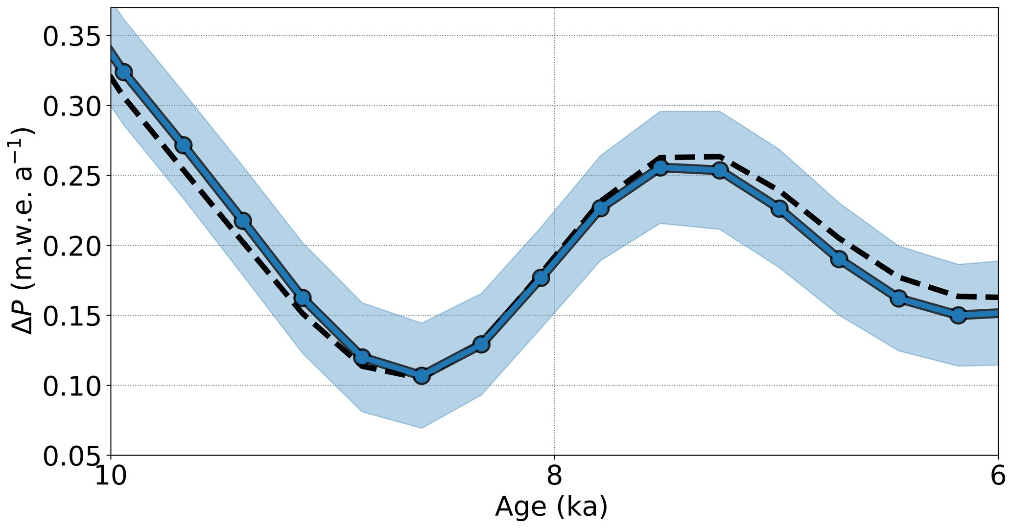
Figure 10The blue line and shaded region show the estimated mean ΔP and 95 % confidence bands, respectively, for the sensitivity test, accounting for uncertainty in a number of ice flow and PDD model parameters. The dashed black line shows the mean estimated ΔP from a previous inversion assuming no uncertainty in model parameters.

Download