the Creative Commons Attribution 4.0 License.
the Creative Commons Attribution 4.0 License.
 | 14 Apr 2020
Multi-physics ensemble snow modelling in the western Himalaya
David M. W. Pritchard
Nathan Forsythe
Greg O'Donnell
Hayley J. Fowler
Nick Rutter
Combining multiple data sources with multi-physics simulation frameworks offers new potential to extend snow model inter-comparison efforts to the Himalaya. As such, this study evaluates the sensitivity of simulated regional snow cover and runoff dynamics to different snowpack process representations. The evaluation is based on a spatially distributed version of the Factorial Snowpack Model (FSM) set up for the Astore catchment in the upper Indus basin. The FSM multi-physics model was driven by climate fields from the High Asia Refined Analysis (HAR) dynamical downscaling product. Ensemble performance was evaluated primarily using MODIS remote sensing of snow-covered area, albedo and land surface temperature. In line with previous snow model inter-comparisons, no single FSM configuration performs best in all of the years simulated. However, the results demonstrate that performance variation in this case is at least partly related to inaccuracies in the sequencing of inter-annual variation in HAR climate inputs, not just FSM model limitations. Ensemble spread is dominated by interactions between parameterisations of albedo, snowpack hydrology and atmospheric stability effects on turbulent heat fluxes. The resulting ensemble structure is similar in different years, which leads to systematic divergence in ablation and mass balance at high elevations. While ensemble spread and errors are notably lower when viewed as anomalies, FSM configurations show important differences in their absolute sensitivity to climate variation. Comparison with observations suggests that a subset of the ensemble should be retained for climate change projections, namely those members including prognostic albedo and liquid water retention, refreezing and drainage processes.
- Article
(5506 KB) -
Supplement
(1593 KB) - BibTeX
- EndNote


Snow plays a profound role in the climate system and supports water resources in many regions (Barnett et al., 2005; Hall and Qu, 2006). As such, several applications depend on process-based models that approximate snow physics while solving mass and energy balances. These include coupled land–atmosphere modelling, testing hypotheses about physical snow processes and catchment behaviour, and hydrological projections in non-stationary climates. Given the number of snow models in existence (e.g. Essery et al., 2013), understanding the relative skill of different models and their suitability for various uses is essential. This is reflected by the succession of snow model inter-comparison initiatives over recent decades (Essery et al., 2009; Etchevers et al., 2004; Krinner et al., 2018; Slater et al., 2001).
While snow models have been evaluated in various contexts, there has been little analysis of how different process-based models perform in the Himalayan region. Yet, vast populations downstream of these water towers are vulnerable to climate change impacts on snowmelt-derived river flows (Immerzeel et al., 2010; Viviroli et al., 2011). Snow model analysis and inter-comparison would ultimately help to manage these risks, but model input and evaluation are severely impeded by data paucity. Indeed, deriving consistent, multivariate climate input fields in largely unobserved and highly variable mountain environments is a long-standing problem (Klemeš, 1990; Raleigh et al., 2015, 2016). In part this explains the proliferation of simple snow modelling in the region, namely through (sometimes enhanced) temperature index methods (e.g. Armstrong et al., 2019; Lutz et al., 2014; Ragettli et al., 2015; Stigter et al., 2017). There are a small but growing number of offline process-based, energy balance model applications (i.e. not coupled to an atmospheric model), but these have focused only on single model structures, without detailed snow process evaluation (e.g. Brown et al., 2014; Prasch et al., 2013; Shakoor and Ejaz, 2019; Shrestha et al., 2015).
In the face of these data challenges, developments in high-resolution regional climate modelling and remote sensing increasingly offer partial solutions. Several studies have now successfully used dynamical downscaling to provide offline forcing for cryospheric and hydrological models in the Himalaya and other contexts (e.g. Biskop et al., 2016; Havens et al., 2019; Huintjes et al., 2015; Tarasova et al., 2016). Similarly, the potential for remote sensing to support model evaluation by providing some constraints on both snow cover dynamics and the surface energy balance has been demonstrated (Collier et al., 2013, 2015; Essery, 2013; Finger et al., 2011). Yet, studies combining these data sources for process-based snow model applications are still few in number (see e.g. Quéno et al., 2016; Revuelto et al., 2018), especially in the Himalaya. Moreover, there has been little examination of how such approaches could support snow model inter-comparison for practical uses, such as water resource modelling and management, as previous inter-comparisons have focused primarily on site scales. More systematic studies are needed to understand differences in snow model behaviour at the larger scales relevant to water resource applications and regional climate modelling (Essery et al., 2009; Krinner et al., 2018).
Although regional climate modelling and remote sensing offer increasing potential to support snow model inter-comparison in data-sparse regions, identifying appropriate model formulations remains challenging even in well-instrumented contexts. In the SnowMIP and SnowMIP2 inter-comparison studies, no single model emerged as optimal, with performance varying between locations and years (Essery et al., 2009; Etchevers et al., 2004; Rutter et al., 2009). Similarly, recent inter-comparisons using more systematic ensemble frameworks have found that different model configurations tend to show consistently good, poor or variable performance, with no single best model identifiable (Essery et al., 2013; Lafaysse et al., 2017; Magnusson et al., 2015). Model complexity, in terms of the number of processes represented and the associated number of parameters, does not appear to be strongly (or necessarily positively) related to skill or transferability in space and time (see also Lute and Luce, 2017). Nevertheless, the systematic frameworks underpinning recent inter-comparisons are an important advance over earlier studies. By synthesising the array of models in existence and eliminating implementation differences, these frameworks permit better quantification of the behaviour of different parameterisations and identification of where improvements may be possible (Clark et al., 2015; Krinner et al., 2018). The full potential of this approach has not yet been realised, especially in data-sparse mountain regions.
Therefore, this study uses recent progress in high-resolution regional climate modelling, remote sensing and ensemble-based snow modelling to assess snowpack model formulations in a western Himalayan catchment. The study proceeds by using the High Asia Refined Analysis (HAR; Maussion et al., 2014) dynamical downscaling product to drive the Factorial Snowpack Model (FSM) multi-physics ensemble (Essery, 2015). The spatially distributed, high-resolution FSM simulations are then evaluated using a combination of multiple MODIS remote-sensing products and local observations. The aim of the study is to evaluate the sensitivity of simulated snow cover and runoff dynamics to different snowpack process representations while also identifying possible causes and implications of model performance variation. This contributes to the need for more large-scale (basin-scale) model evaluations using unified frameworks (Clark et al., 2015; Essery et al., 2013) in a context where accurately simulating snow processes is essential for understanding cryospheric, hydrological and water resource trajectories in a changing climate.
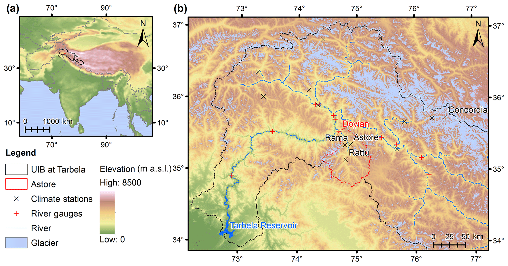
Figure 1Location of study area and local measurement points. The regional context is indicated in (a). The Astore catchment and observation locations (with labels for the most important sites in this study) are shown with topography and glacier extent in (b). The SRTM 90 m DEM v4.1© (Jarvis et al., 2008) and Randolph Glacier Inventory 5.0© (Arendt et al., 2015) datasets are both licenced under a Creative Commons Attribution 4.0 International License (CC BY 4.0).
The study focuses on the steep, mountainous Astore catchment, a 3988 km2 gauged sub-basin of the upper Indus basin (Fig. 1). The mean elevation of the catchment is around 4000 m a.s.l., with 57 % and 87 % of the area lying in the elevation ranges 3500–4500 and 3000–5000 m a.s.l., respectively. River flows are typically very low in winter, before rising in spring and peaking in summer (June–July). Spring and summer runoff is dominated by snowmelt, which is derived primarily from orographically enhanced snowfall in the preceding winter and early spring (Archer, 2003). Showing notable spatial correlation at the seasonal scale, much of this snowfall originates from synoptic-scale low-pressure systems known as westerly disturbances (Archer and Fowler, 2004). Monsoon influences are small compared with the central Himalaya. Together with the fact that glacier cover is relatively limited, at around 6 % according to the Randolph Glacier Inventory 5.0 (Arendt et al., 2015), the strong correlation between winter precipitation and summer river flows indicates that catchment runoff is primarily mass- rather than energy-limited (Archer, 2003; Fowler and Archer, 2005). However, energy constraints certainly affect intra-seasonal variability. The perennial snowpack that persists through the summer is confined to small areas of very high elevation, while the glaciated extent is sufficient only to provide a modest contribution to late-summer river flows (Forsythe et al., 2012). The ESA GlobCover 2009 product (Arino et al., 2012) indicates that vegetation cover is relatively sparse, with the catchment dominated by a mixture of bare ground, herbaceous plants, and perennial snow and ice.
3.1 Model
3.1.1 Factorial Snowpack Model (FSM) overview
FSM is an intermediate-complexity, systematic framework for evaluating alternative representations of snowpack processes and their interactions (Essery, 2015). Constructed around a coupled mass and energy balance scheme, FSM was originally formulated as a one-dimensional column model with up to three layers, depending on the total snow depth. The model is based on the sequential solution of a set of linearised equations at each time step. The surface energy balance is solved first. Turbulent heat fluxes are estimated using the bulk aerodynamic approach. Heat conduction between layers and to the substrate is calculated using an implicit scheme before layer ice and water masses are updated to account for simulated rainfall, melt, sublimation, refreezing, drainage to successive layers and runoff from the base of the snowpack. FSM then updates layer densities and thicknesses, accounting for snowfall and conservation of total ice and liquid water masses as well as internal energy.
Table 1Summary of the process parameterisation options available in FSM. Full details are provided in Essery (2015). The short names and abbreviations by which the processes are referred to in the text and figures are given.
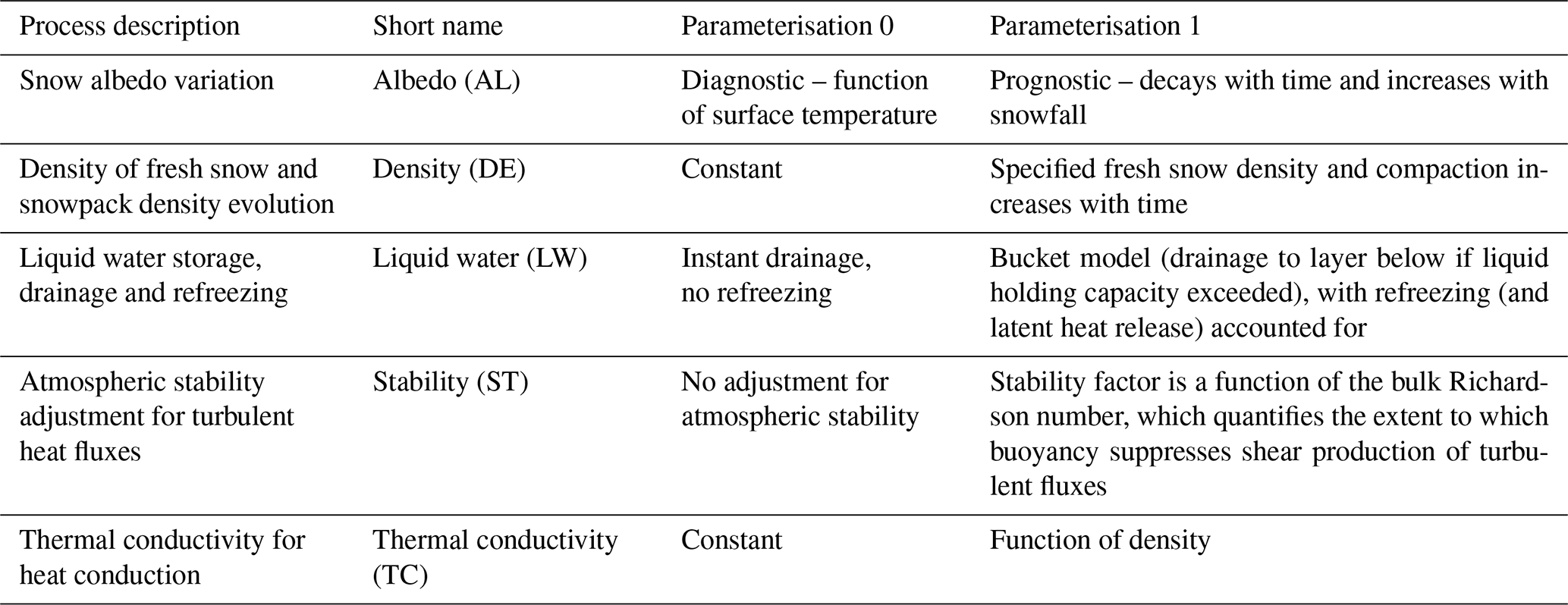
Within this framework, FSM offers alternative parameterisations of different snowpack processes. The five processes are as follows: (1) albedo evolution; (2) thermal conductivity variation; (3) snow density change by compaction; (4) adjustment of turbulent heat fluxes for atmospheric stability; and (5) liquid water retention, refreezing and drainage. With two parameterisation options (0 or 1) for these five processes, the FSM ensemble includes 32 possible model configurations. Summarised in Table 1, the options synthesise approaches found in a range of widely applied models. These include CLASS (Verseghy, 1991), CLM (Oleson et al., 2013), Crocus (Vionnet et al., 2012), HTESSEL (Dutra et al., 2010), ISBA (Douville et al., 1995), JULES (Best et al., 2011), MOSES (Cox et al., 1999) and Noah-MP (Niu et al., 2011). For each process, the second option (1) may be considered generally more physically realistic (i.e. more in line with conceptual understanding of the physical processes governing snowpack evolution) than the first option (0). For example, in the case of snowpack hydraulic processes, it is more realistic to include liquid water retention, refreezing and drainage via a bucket model (option 1) than to permit instantaneous drainage of liquid water instead (option 0).
Analyses of FSM to date have shown that it gives ensemble performance and spread comparable to larger multi-model ensembles (Essery, 2015). As such, it has been used to support study design and inter-comparison in the ESM-SnowMIP initiative (Krinner et al., 2018). Its value for testing new process representations in forest environments has also been demonstrated (Moeser et al., 2016), while Günther et al. (2019) used FSM to delineate the influences of input data errors, model structure and parameter values on simulation performance at an Alpine site.
3.1.2 Adaptations and implementation
While the core FSM subroutines used in this study remain as described in Essery (2015), the model was adapted to perform spatially distributed simulations on a regular grid, using climate inputs that vary in space and time. In this adaptation, each grid cell is treated as independent of all other cells. Inter-cell mass and energy transfers are not considered, but the default parameterisation of sub-grid variability of snow cover as a function of snow depth is retained. In effect, each grid cell is considered to be a site for which the original FSM formulation is run. The adapted version of the model is thus similar in principle to other widely applied, distributed snow models when used without their snow transport options (Lehning et al., 2006; Liston and Elder, 2006a; Marks et al., 1999). In line with the focus on snow cover dynamics and snowpack processes, the model does not simulate other aspects of catchment hydrology, such as evapotranspiration from snow-free cells, the soil water balance or hydrological routing (subsurface, overland and channel flows).
The simulations reported here use a 500 m horizontal resolution grid and an hourly time step. Topography is derived from the Shuttle Radar Topography Mission (SRTM) 90 m digital elevation model (DEM) v4.1 (Jarvis et al., 2008). The 500 m spatial resolution is representative of hydrological and cryospheric modelling applications in the large basins of the Himalaya (e.g. Lutz et al., 2016) as well as extremely high resolution climate modelling (e.g. Bonekamp et al., 2018; Collier and Immerzeel, 2015). It is also consistent with several of the MODIS products used for evaluation (Sect. 3.3). Spatial variation in land surface properties is ignored on the basis that glacier and vegetation (including forest) cover is low (Sect. 2) and information on substrate properties is unavailable. The simulations use the default FSM model parameters, which have been shown to reproduce much of the spread in previous model inter-comparisons (Essery, 2015).
3.2 Climate inputs
3.2.1 High Asia Refined Analysis (HAR)
Spatiotemporally varying input fields of rainfall, snowfall, air temperature, relative humidity, wind speed, surface air pressure, and incoming shortwave and longwave radiation are based on the HAR (Maussion et al., 2014). The HAR is a 14-year dynamical downscaling of coarser global analysis to 10 km over the Himalaya and Tibetan Plateau using the Weather Research and Forecasting (WRF) model (Skamarock et al., 2008). Although a seasonally varying cold bias is present in the upper Indus basin, the HAR shows substantial performance in capturing many spatial and temporal patterns in the near-surface climatology (Maussion et al., 2014; Pritchard et al., 2019). The HAR has also exhibited a good representation of climate in several hydrological and glaciological modelling studies in neighbouring regions (Biskop et al., 2016; Huintjes et al., 2015; Tarasova et al., 2016).
3.2.2 Bias correction and downscaling
Near-surface air temperature fields were bias-corrected to reduce the HAR's cold bias in the study area. The mean bias was estimated using quality-controlled local observations from stations in the Astore catchment (Fig. 1b), which are maintained by the Pakistan Meteorological Department (PMD) and the Water and Power Development Authority (WAPDA). Typical of data-sparse high-mountain regions, the available stations are situated in valley locations. The HAR cold bias relative to these stations has been shown to be closely related to issues in snow cover representation in the WRF simulations underpinning the HAR (Pritchard et al., 2019), but some influence of local meteorological processes such as cold air drainage cannot be ruled out, at least at some sites. More advanced bias correction approaches were tested, including quantile-based methods, but these did not lead to improvements either in cross validation at station locations or model performance at the catchment scale. This is likely due to the difficulty of fully characterising spatial and temporal variation in biases based on limited observations, especially for less commonly measured variables. The minimal approach taken thus represents a realistic application of the data. It also has the advantage of retaining much of the physical consistency of the HAR fields in terms of both inter-variable and spatiotemporal dependence structures.
For most of the climate variables, spatial disaggregation of the 10 km HAR fields to the 500 m FSM grid was conducted using methods similar to those in the MicroMet meteorological pre-processor of SnowModel (Liston and Elder, 2006b) and those used by Duethmann et al. (2013). Specifically, for temperature, specific humidity, incoming longwave radiation, pressure and (log-transformed) precipitation, linear regression was used each time step to relate each variable to elevation, based on all HAR grid cells within the catchment (i.e. by regressing the simulated surface – or near-surface – values against the elevations of the corresponding model grid cells). If the gradient term in the regression was significant at the 95 % confidence level, the values at each HAR cell (10 km grid) were interpolated to a reference level using the gradient. This spatial (horizontal) anomaly field was then interpolated to the high-resolution FSM grid (500 m), and the elevation signal was subsequently reintroduced using the regression gradient. This approach thus differs from MicroMet primarily by using gradients that can vary at each time step rather than applying a single climatological gradient for each calendar month. For time steps when the gradient term in the regression was not statistically significant, simple interpolation of the HAR field to the FSM grid was undertaken.
Due to the pronounced topography of the study area, clear-sky shortwave radiation at the surface was estimated for the 500 m resolution DEM using a vectorial algebra approach (Corripio, 2003). This approach accounts for the effects of slope, aspect, hill-shading and sky view factor. It has been successfully applied before in this region (e.g. Ragettli et al., 2013) and was additionally checked against station measurements. The calculated clear-sky shortwave radiation fields were adjusted to account for HAR-simulated cloud cover effects. The cloud cover effects were estimated by using spatially interpolated ratios of all-sky to clear-sky incoming shortwave radiation at the surface, with both quantities from the HAR. This approach maintains consistency between variables while capturing topographic influences, although direct and diffuse partitioning and cloud variability are simplified. In addition, MicroMet itself was used to downscale wind speed to the 500 m grid to take advantage of MicroMet's routines for modulating wind fields according to topographic slope and curvature.
3.2.3 Uncertainty
Given the low density of climate observations, biases and other errors undoubtedly remain in the climate input fields. As such, two alternative input strategies were tested. The first strategy uses the same approach outlined in Sect. 3.2.2 but simply forgoes bias correction of temperature. The second strategy retains the same approaches for precipitation, incoming shortwave radiation and wind speed, but local observations from the Astore and other catchments in the north-western upper Indus basin (Fig. 1b) are used to estimate fields for the other required variables (temperature, humidity and incoming longwave radiation – see Sect. S1 in Supplement). The purpose of these two alternative strategies is to indicate whether the main conclusions reached on snowpack process representations are unduly affected by the approaches described in Sect. 3.2.2.
3.3 Model evaluation
The model evaluation focuses primarily on snow cover dynamics, with other variables considered to evaluate underlying processes. Typical of the remote Himalaya, no local snow measurements for site-scale evaluation were available. The evaluation thus uses a number of MODIS remote-sensing products (Collection 6) to assess the FSM ensemble over the full simulation period (October 2000 to September 2014). These include snow-covered area (SCA) derived from the MOD10A1 daily snow cover product (Hall and Riggs, 2016). Data with quality flags of 0 (best), 1 (good) and 2 (OK) were retained, and the widely used cloud infilling method developed by Gafurov and Bárdossy (2009) was then applied. The analysis focuses primarily on SCA corresponding with a normalised difference snow index (NDSI) threshold of zero. This indicates very limited or no snow cover in a pixel (Salomonson and Appel, 2004), which is consistent with the no-snow threshold used to calculate modelled SCA.
In addition, comparisons with MOD11A1 land surface temperature (LST) are undertaken. To extend previous validations (e.g. Wan, 2014; Wan et al., 2004), an evaluation of MOD11A1 at the Concordia site (Fig. 1b) in the neighbouring Karakoram range is given in the Supplement (Sect. S2). The evaluation shows that the product performs well compared with observed surface temperatures, with a relatively low mean bias of −0.55 ∘C. Spatial aggregates for LST were only calculated when 90 % of pixels had satisfactory quality retrievals, which are defined here as mandatory data quality flags of 00 (good). Additional evaluation of the FSM albedo parameterisations presented in the Supplement also draws on the MCD43A3 and MOD10A1 surface albedo products, as detailed in Sect. S3.
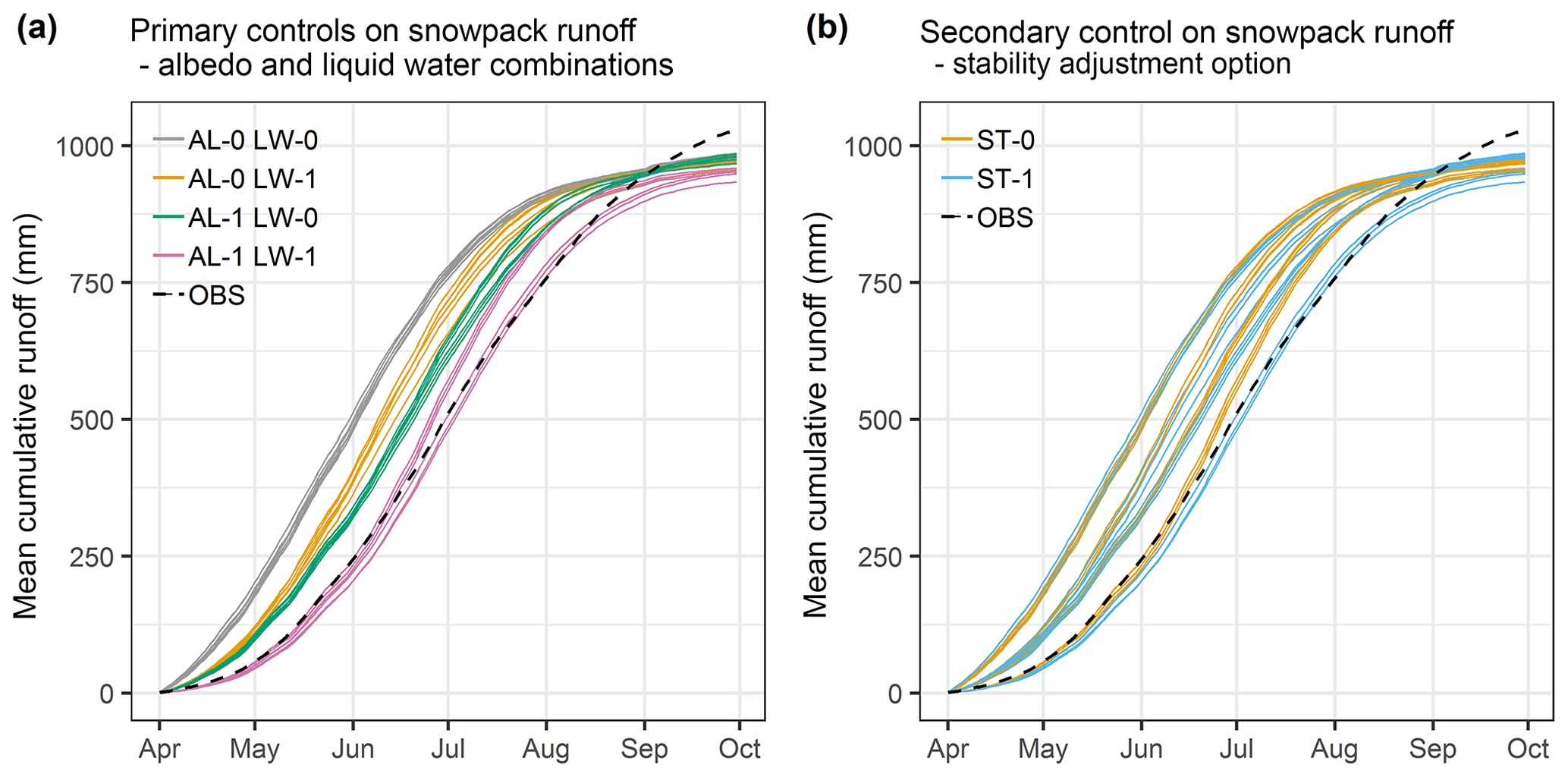
Figure 2Mean cumulative snowpack runoff for the high-flow season for each of the 32 ensemble members. In (a) each ensemble member is coloured according to the combination of albedo (AL) and liquid water (LW) parameterisations it uses. In (b) each ensemble member is coloured by its stability adjustment (ST) option. Observed total runoff (OBS; black dashed line) is shown for reference only (it is not directly comparable with snowpack runoff – see Sect. 3.3).
The study also uses quality-controlled daily river flows over the period October 2000 to September 2010 recorded at the Doyian gauging station by WAPDA (Fig. 1b). These data are used to provide some context on the volume, timing and variability of catchment runoff. As the adapted FSM model does not simulate full catchment hydrology (Sect. 3.1.2), the use of the observed data is restricted to two cases: (1) an indication of the timing of the rising limb of the annual hydrograph (and thus the timing of early snowpack runoff) for context and (2) an indication of the sensitivity of runoff to climate variability in the snow-dominated earliest part of the melt season (April), when flow pathways from the low-elevation melting snowpack to the main channels are short, travel times are low and the influence of evapotranspiration is relatively small (Lundquist et al., 2005; Naden, 1992). The modelled quantity considered is termed snowpack runoff, which is defined as runoff from the base of the snowpack. It is thus different to surface melt, which may be subject to storage and refreezing processes before leaving the snowpack. Snowpack runoff is aggregated across all grid cells in the catchment (or across subsets of the cells for selected analyses) without any routing.
4.1 Mean ensemble structure
4.1.1 Snowpack runoff
The evaluation begins by considering how the FSM ensemble is structured on average at the catchment scale. For snowpack runoff (as defined in Sect. 3.3), the ensemble shows notable spread, which takes the form of groupings of ensemble members (Fig. 2). Three groups of cumulative snowpack runoff curves are distinguishable early in the melt season (April and early May) in Fig. 2, but the groups split and their spread increases to varying degrees thereafter, as melt rates accelerate. Differences in snowpack runoff timing between groups are substantial, with variation of around 1 month in the date at which the 25th, 50th and 75th percentiles of total seasonal snowpack runoff are exceeded.
Figure 2a indicates that the development of groups in the ensemble is primarily controlled by interactions between parameterisations of albedo and liquid water processes within the snowpack. The earliest, most rapid snowpack runoff occurs for members combining diagnostic albedo with instantaneous liquid water drainage (grey in Fig. 2a). In contrast, the slowest-responding members (purple in Fig. 2a) use prognostic albedo and apply the parameterisation of liquid water retention, refreezing and drainage processes (hereafter referred to as the liquid water parameterisation). The remaining two combinations of albedo and liquid water representations result in similar cumulative runoff curves, especially early in the season (orange and green in Fig. 2a). This indicates that a propensity for earlier, more rapid runoff when applying diagnostic albedo is offset by a delaying effect of the liquid water parameterisation. Conversely, a tendency to delay runoff in the prognostic albedo parameterisation is counteracted by faster runoff due to instantaneous drainage. Interactions between the albedo and liquid water parameterisations thus appear to govern whether a given option's tendency to accelerate or slow snowpack runoff is compensated for or exacerbated.
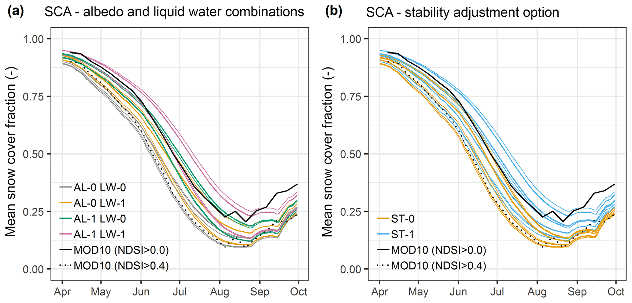
Figure 3Similar to Fig. 2 but for catchment snow-covered area (SCA). The two MODIS MOD10A1 series shown are based on normalised difference snow index (NDSI) thresholds of 0.0 (solid line) and 0.4 (dotted line).
The next most important determinant of ensemble structure for snowpack runoff is the stability adjustment option, whose significance increases later in the melt season, especially in July. As noted above, Fig. 2a indicates that the spread in the ensemble groups increases with time. Cross-referencing this with Fig. 2b illustrates that the stability adjustment is the main driver of the divergence. The separation is particularly pronounced for the slowest-responding ensemble members (purple in Fig. 2a). In this case, not applying a stability adjustment leads to more rapid snowpack runoff from mid-June and earlier convergence with the other ensemble members, as evident from comparing the lowermost orange and blue curves in Fig. 2b. In contrast, the adjustment effect is much less pronounced for the faster-responding groups of ensemble members in Fig. 2a (grey curves). Therefore, sensitivity to the stability adjustment not only varies notably through the melt season but is also a function of the choices of albedo and liquid water parameterisations.
4.1.2 Snow-covered area (SCA)
Figure 3 indicates that the albedo, liquid water and stability adjustment parameterisations are also the main influences on mean ensemble spread and structure in SCA. However, the dominance of albedo and liquid water processes is lesser compared with snowpack runoff, especially later in the melt season. By the annual SCA minimum in August, the stability adjustment comes to control ensemble structure (Fig. 3b). Model configurations applying the adjustment exhibit a markedly slower decline in SCA over the melt season, which leads to an annual SCA minimum approximately 5 % higher. Spatially, this difference is largely found at high elevations (not shown), which could have substantial implications for modelling the evolution of ice mass in the catchment over longer periods. However, these high-elevation areas are also particularly subject to the influences of blowing-snow processes and avalanching, which typically alter high-elevation snow cover patterns (see discussion in Sect. 5.2).
For much of the melt season, the model configurations most closely matching MODIS SCA (using an NDSI threshold of zero – see Sect. 3.3) apply prognostic albedo, along with either no liquid water representation but a stability adjustment or the liquid water parameterisation but no stability adjustment. The similar responses of these two combinations of liquid water and stability adjustment parameterisations again reflect compensatory effects in the ensemble. Switching on the liquid water representation slows the rate of SCA decline, while turning off the stability adjustment speeds it up, and vice versa. Therefore, turning off the stability adjustment compensates for the tendency for slower SCA decay when using the liquid water parameterisation, whereas turning on the stability adjustment compensates for the tendency for faster SCA decline when assuming instantaneous drainage of liquid water from the snowpack. For most of the other ensemble members, the SCA curves exhibit a relatively rapid snow cover decline during the melt season compared with MODIS (NDSI threshold of zero). Section S4 in the Supplement explores how differential SCA errors could relate to differences in the timing of early-season simulated snowpack runoff and observed total runoff as well as what this could imply about the hydrological behaviour of the catchment.
Table 2Catchment-scale mean differences (option 1 minus option 0) for key states and fluxes in selected months. Differences are calculated separately for the albedo (AL), liquid water (LW) and stability adjustment (ST) parameterisations. Albedo differences are at solar noon, and average snowpack temperatures are weighted by snow depth.

4.2 Process evaluation
The analysis now explores the processes behind the structure of ensemble spread identified in Sect. 4.1 as well as how far they can be assessed with independent data. This assessment is based in part on Table 2, which summarises the mean influences of albedo, liquid water and stability adjustment parameterisation choices on key catchment-scale states and fluxes in selected months. The influences are delineated as the monthly mean differences between those ensemble members applying one option for a given process (e.g. prognostic albedo) and those members applying the other option (e.g. diagnostic albedo). Density and thermal conductivity parameterisations are not considered, as it can be inferred from Sect. 4.1 that their effects are comparatively minor for the foci of this study, namely SCA and snowpack runoff.
4.2.1 Albedo
Table 2 shows that prognostic albedo in FSM tends to be higher than diagnostic albedo in the first part of the melt season. The mean difference between the two albedo options ranges from 0.12 to 0.15 between April and June at solar noon. The resulting difference in net shortwave radiation helps to explain why prognostic albedo initially delays and slows melt, snowpack runoff and SCA decline relative to diagnostic albedo, which ultimately permits more snowpack runoff later in the season (see Sect. 4.1 and Table 2). One factor in the faster melt in spring and early summer using diagnostic albedo is its pronounced diurnal range. This is linked to the diurnal surface temperature cycle, partly through a positive feedback. The mean diurnal range in albedo for daylight hours rises from 0.18 to 0.27 between April and June when using the diagnostic parameterisation, whereas the equivalent range for the prognostic parameterisation stays much lower, at around 0.02. While albedo does vary diurnally with solar zenith angle, it does not necessarily follow that the diagnostic parameterisation captures the magnitude of variation appropriately. Section S3 in the Supplement demonstrates that the prognostic parameterisation agrees better with the MODIS albedo products than the diagnostic option, as might be expected from previous studies (e.g. Essery et al., 2013).
4.2.2 Liquid water retention, refreezing and drainage
Table 2 shows that the net effect of switching on the liquid water parameterisation is to delay snowpack runoff even though it accelerates surface melt rates. For example, in April (May), snowpack runoff is on average 1.9 mm d−1 (1.6 mm d−1) lower when using the liquid water parameterisation, even though surface melt is 1.0 mm d−1 (1.9 mm d−1) higher. With the option on, liquid water from melting is allowed to refreeze, leading to latent heat release, which maintains a higher snowpack temperature (for example by 3.5 ∘C in April). Retention and delayed release of liquid water in storage are part of the reason why these higher temperatures lead to higher melt rates but not higher snowpack runoff rates initially. However, multiple diurnal cycles of melting and refreezing may also be required before a given unit of snow is entirely converted to snowpack runoff. At any rate, the delaying effect of switching on the liquid water option outweighs its tendency to increase melt rates in this setting. By allowing snow to persist for longer, this enhanced storage ultimately leads to higher melt and runoff rates later in the season (by July), as later-lying snow becomes subject to increasing energy inputs (e.g. Musselman et al., 2017).

Figure 4Comparison of modelled seasonal mean elevation profiles of LST with MODIS MOD11A1 remote sensing. The ensemble members are grouped by stability adjustment option (mean and range of groups shown). The top (a–d) and bottom (e–h) rows show night-time and day-time temperatures, respectively. Model results correspond with the closest model time step to the Terra platform overpass times as well as only days for which MODIS retrievals are available (i.e. clear-sky conditions).
4.2.3 Stability adjustment
Table 2 also demonstrates that switching on the stability adjustment leads to lower melt rates later in the season, primarily due to a smaller sensible heat flux towards the snow surface in stable atmospheric conditions. During the early part of the season (e.g. April), the differences in net turbulent fluxes arising from the stability adjustment choice (16 W m−2) are largely offset by differences in net radiation (12.3 W m−2). The larger sensible heat flux to the surface with no stability adjustment leads to a higher surface temperature (by 2.9 ∘C in April) and thus higher outgoing longwave radiation, which incurs lower net longwave radiation. However, as the gradients between the snow surface (limited to 0 ∘C) and near-surface air temperatures increase in spring and summer, the differences in net turbulent fluxes ultimately drive differences in the surface energy balance and melt rates. By June and July, the differences in net radiation (16 and 20 W m−2) no longer offset the differences in net turbulent fluxes (36.8 and 52.7 W m−2). Yet, Table 2 also indicates that the resulting differences in melt rates do not necessarily alter snowpack runoff on average. This reinforces the point that modelled snowpack runoff sensitivity to the stability adjustment is contingent on the representations of other processes, namely albedo and liquid water retention, refreezing, and drainage (Sect. 4.1.1). It is also noteworthy that switching on the stability adjustment approximately halves average sublimation from 80 to 45 mm yr−1, which corresponds with around 8 % and 4 % of total catchment snow ablation, respectively.
While data to evaluate turbulent fluxes directly are not available, Fig. 4 shows that switching off the stability adjustment leads to higher LST, which is in fact in closer agreement with MODIS LST. This is somewhat counter to initial expectations, as applying a stability adjustment would typically be considered more physically realistic. The largest differences in vertical LST profiles occur at night and increase with elevation for the clear-sky conditions when MODIS retrievals are available. These differences may suggest too strong a suppression of turbulent fluxes under stable conditions using the bulk Richardson number correction. Such suppression may well contribute to the slow SCA decline when combining the stability adjustment with the otherwise realistic configuration of prognostic albedo and the parameterisation of liquid water processes (Sect. 4.1). Ensemble spread in day-time LST is smaller and generally in good agreement with MODIS, although the extent and influence of sub-pixel snow cover variation on MODIS LST likely increases during melting periods, giving it some positive bias in summer (Sect. S2 in Supplement).
4.3 Spatial variation in process sensitivity
Figure 5 examines how the tendencies identified in Sect. 4.1–4.2 are manifest spatially as well as how the influence of different processes depends on both space and time. Spatial (vertical) and temporal (monthly) differences in simulated snowpack runoff due to albedo, liquid water processes and stability option choices are shown. The differences are calculated as option 1 minus option 0 for each process, with the former being generally considered more realistic (Sect. 3.1.1). The lines in Fig. 5 show mean differences, while ranges denote inter-annual variability. Monthly mean freezing isotherm elevations for daily minimum, mean and maximum temperatures are shown to help interpret the vertical patterns.
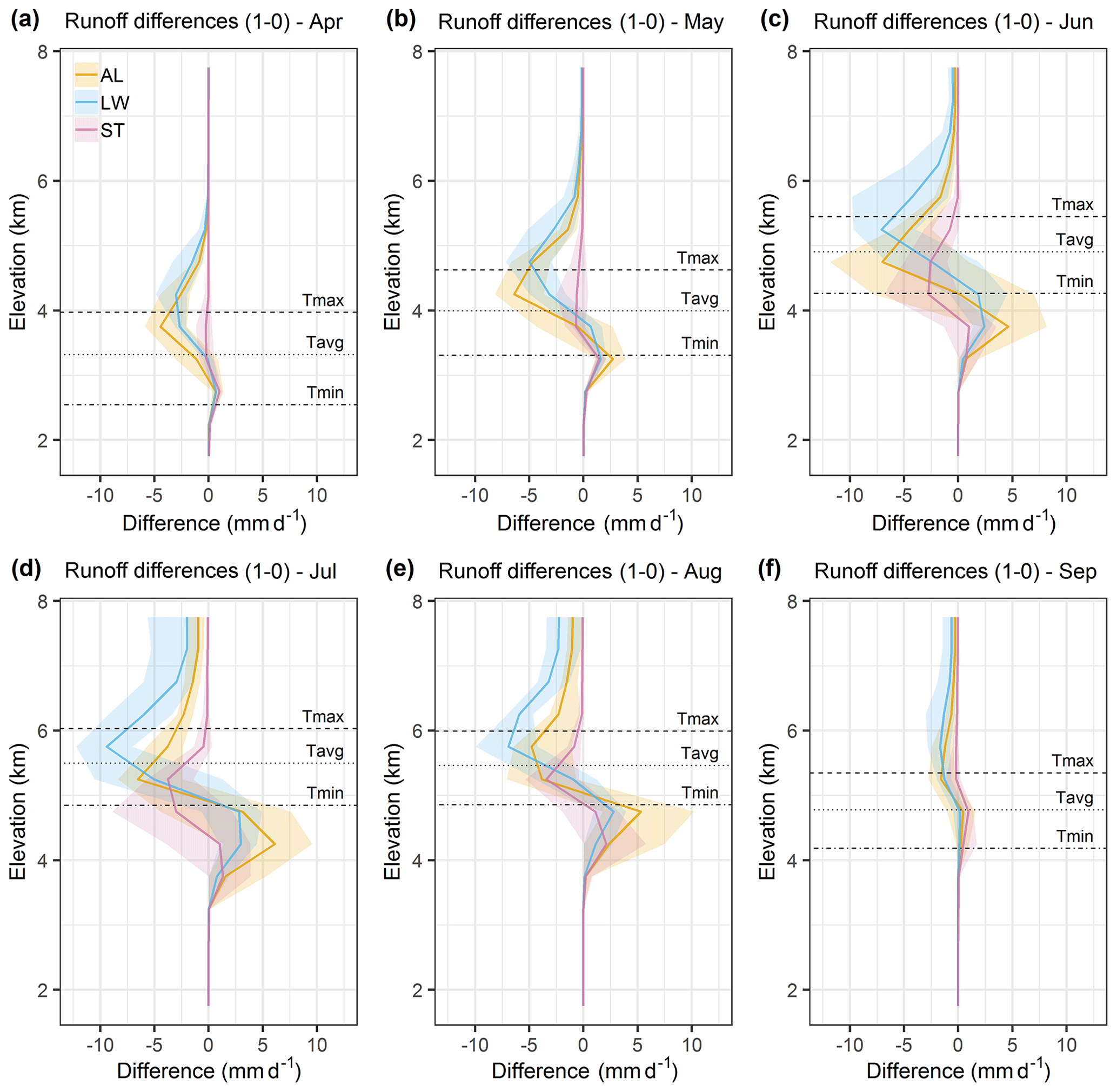
Figure 5Spatial (vertical) and temporal (monthly) differences in simulated snowpack runoff as a result of albedo (AL), liquid water (LW) and stability option (ST) choices. The differences are calculated as option 1 minus option 0 for each process. Lines show mean differences, while ranges denote inter-annual variability. Monthly mean freezing isotherm elevations for daily minimum, mean and maximum temperatures are also shown.
Figure 5 shows that S-shaped vertical profiles of snowpack runoff differences develop and migrate upwards as the melt season progresses. The profiles take this form because the 0 options in FSM for albedo, liquid water and stability adjustment parameterisations all lead to earlier and larger snowpack runoff and snow water equivalent (SWE) depletion relative to the 1 options (see Table 1 and Sect. 4.1–4.2). This gives negative differences earlier in the season at higher elevations when energy availability exerts more control over melt rates. However, it also means that the 1 options (i.e. prognostic albedo, liquid water processes represented and stability adjustment applied) are associated with larger SWE later in the season, allowing more runoff at lower elevations (positive differences in Fig. 5 increasing through the season). This is consistent with the catchment responses described above, although the inter-annual variation in the magnitude of differences is notable.
The S-shaped profiles for the different processes migrate upwards through the melt season in sequence. The profile for (negative) differences due to liquid water processes peaks at the highest elevations, followed by the albedo and then the stability adjustment profiles. The choice of liquid water option is particularly critical around the freezing isotherm for daily maximum temperatures, determining whether early melt is released from the snowpack or subject to storage through refreezing–melting cycles (Sect. 4.2.2). In comparison, the lower elevation of peak negative differences caused by the albedo parameterisation reflects the sensitivity of the diagnostic option to the higher snow surface temperature found under higher daily mean air temperatures. The peak negative differences due to the stability adjustment option are found at lower elevations again, reflecting their dependence on the development of large near-surface temperature gradients (Sect. 4.2.3). Notably, for both albedo and particularly liquid water processes, differences in snowpack runoff are present up to the highest elevations. Therefore, how these processes are represented is critical for simulating the fate of high-elevation perennial snow and ice.
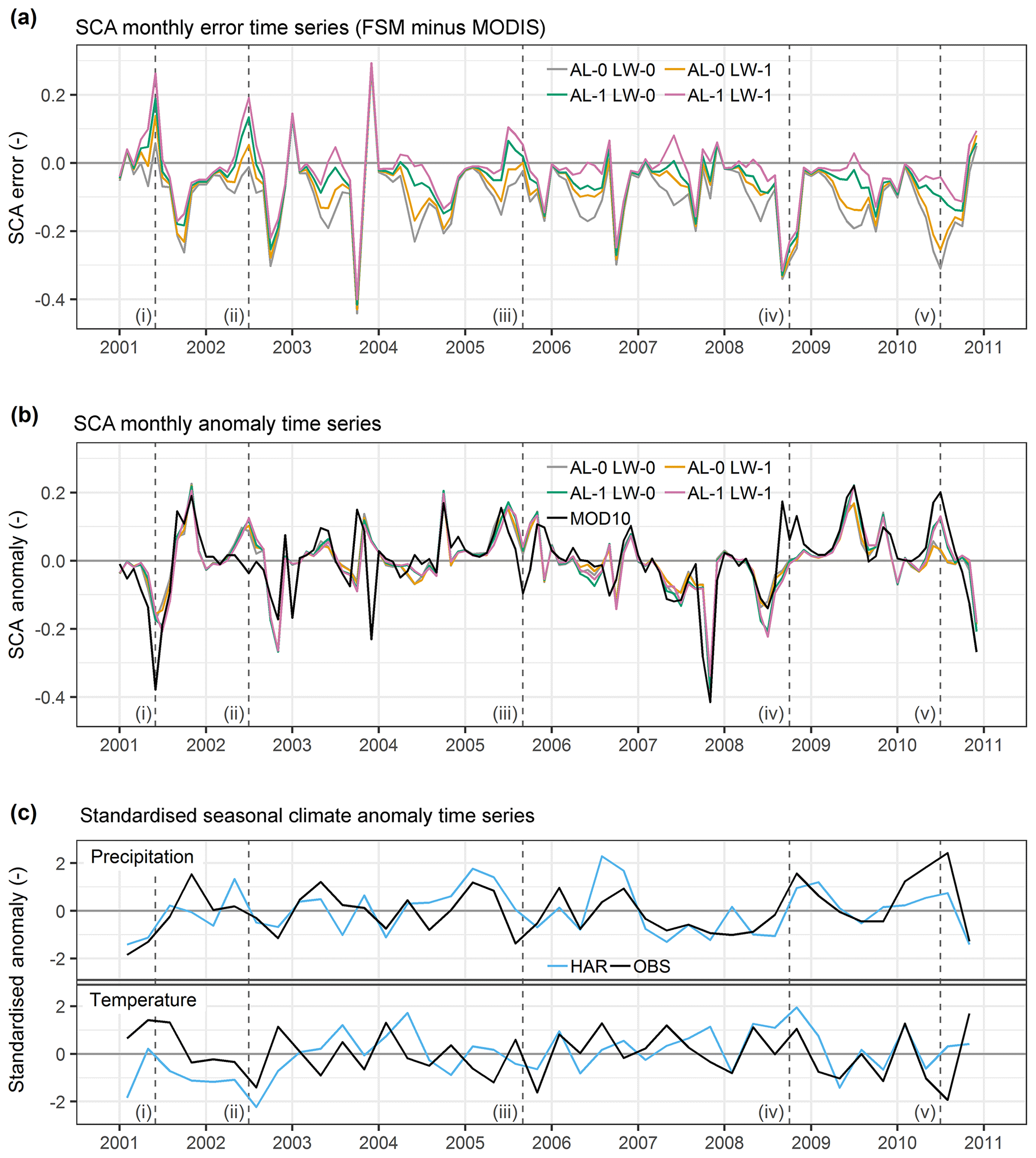
Figure 6Comparison of model SCA performance in absolute and anomaly space with climate inputs. Monthly time series show (a) SCA errors relative to MOD10A1 (FSM minus MODIS) and (b) anomalies (subtracting monthly means from absolute SCA) after aggregating the ensemble by the combinations of albedo and liquid water parameterisations. Standardised seasonal precipitation and temperature anomalies based on observations aggregated from the climate stations in Fig. 1b and the HAR are given in (c).
4.4 Temporal variation in ensemble structure and performance
Figure 6a shows time series of absolute catchment SCA errors (calculated as FSM minus MODIS). This series demonstrates that the best-performing group of configurations varies both between and within years but that the structure of the ensemble remains fundamentally similar between years. Specifically, while the groups of FSM configurations all converge in winter, their divergence in spring and summer follows a similar pattern each year. The group using prognostic albedo and the liquid water parameterisation is consistently the uppermost series in Fig. 6a, while the group using diagnostic albedo and no liquid water parameterisation is consistently the lowermost. The rank order of the groups remains the same through time, although the magnitude of divergence varies notably between years. In some years, fast-responding combinations (Sect. 4.1) exhibit the lowest overall errors in at least part of the melt season (for example 2001, 2002, 2005 and 2007). Autumn convergence of groups is often associated with larger SCA errors due to limitations of the climate inputs in capturing specific snowfall and melt events.
Despite these patterns of divergence and variation in absolute errors, Fig. 6b indicates that, when transformed to anomaly series, the different FSM configurations are generally much more consistent, both with each other and with remote sensing. Anomalies were calculated by subtracting the mean SCA for each month from the absolute SCA separately for MODIS and the ensemble groups (Sect. 3.3). The sign and magnitude of SCA anomalies are generally well simulated, and the range in anomalies shown in Fig. 6b is clearly much smaller than the range of absolute errors during spring and summer in different configurations (Fig. 6a). While the focus here is on SCA, as the comparison with MODIS is fairly direct, similar findings are also evident for snowpack runoff and LST, as shown in the Supplement (Sect. S5). With potentially important implications for seasonal forecasting, this reflects the critical role of climatic drivers in shaping the response of diverse snow models.
Table 3Assessment of SCA time series errors in Fig. 6 and their relationships with climate anomalies. Error IDs correspond with Fig. 6.
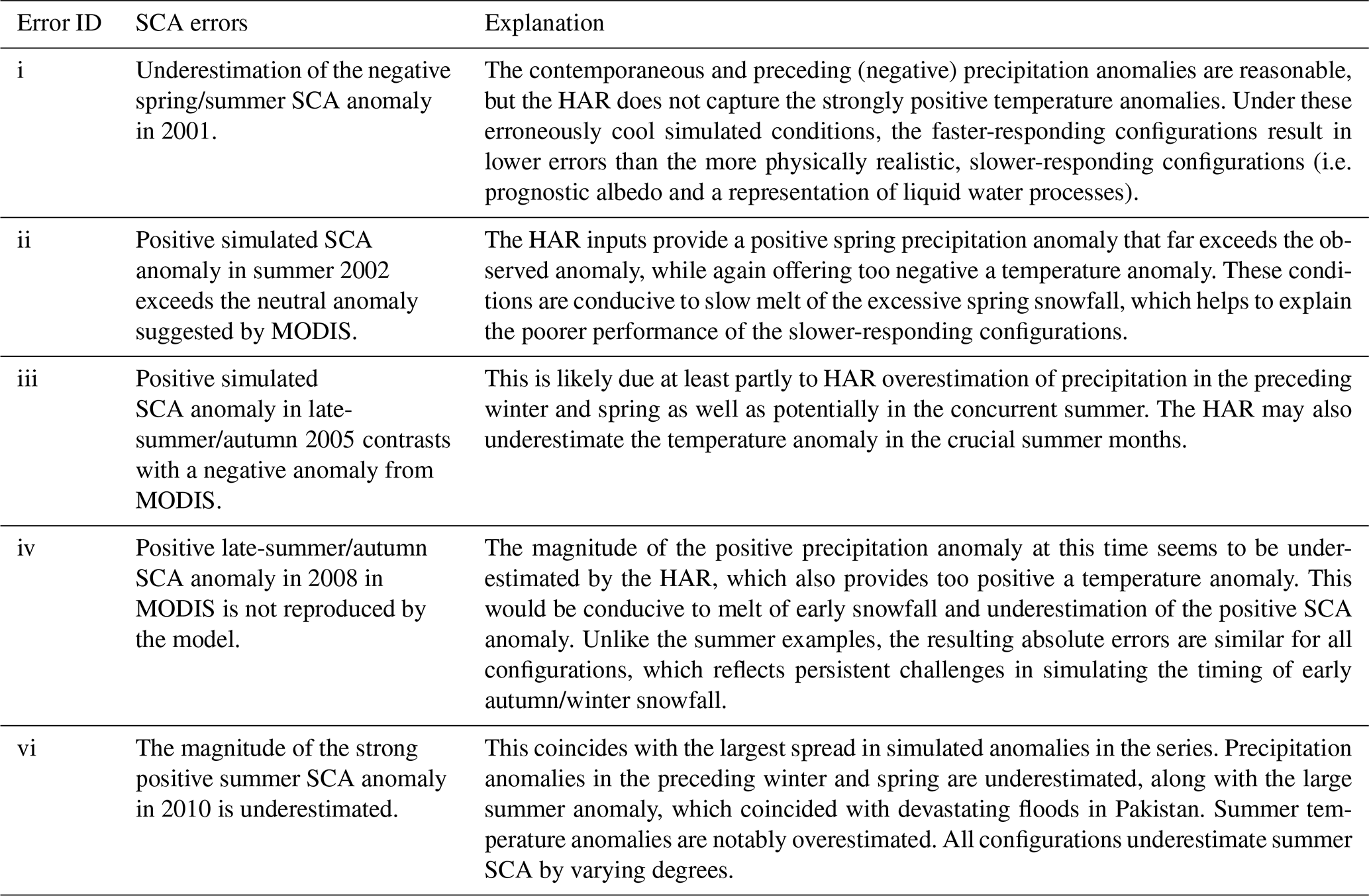
However, Fig. 6b also shows that there are some instances where errors are still large in anomaly space. To explore whether these errors could be due to climate inputs, rather than model response, Fig. 6c provides time series of seasonal precipitation and temperature anomalies from the HAR input data product and local observations. As noted in Sect. 2, local observations show strong spatial correlation at the seasonal scale (Archer and Fowler, 2004; Archer, 2004). While the HAR provides reasonable climatological performance in many respects (Sect. 3.2.1), Fig. 6c suggests that its agreement with observed seasonal climate anomalies is quite variable. Taking the underestimation of the negative SCA anomaly in spring–summer 2001 in Fig. 6b as an example (labelled as (i) in Fig. 6), Fig. 6c indicates that HAR precipitation anomalies in the (preceding) winter and (contemporaneous) spring and summer are reasonable but that the positive observed temperature anomalies are substantially underestimated by the HAR. The erroneously cool conditions would be conducive to relatively slow simulated melt rates. This helps to explain the anomaly error as well as the large absolute SCA error in the slower-responding, more physically realistic configurations in Fig. 6a (i.e. prognostic albedo with representation of liquid water processes).
Table 3 details more such examples. Together, these cases strongly suggest that the larger discrepancies between modelled and remotely sensed SCA anomalies may be related to issues with the sequences of climate input anomalies. Importantly, the examples also generally imply that nudging the climate anomalies towards observations would lead to reduction of absolute errors for the more physically realistic configurations, similar to example (i) discussed above. Thus, there is evidence that errors in climate input anomalies are a substantial factor in performance variation for FSM configurations in the Astore catchment, which partly explains poor performance of more realistic models in some years.
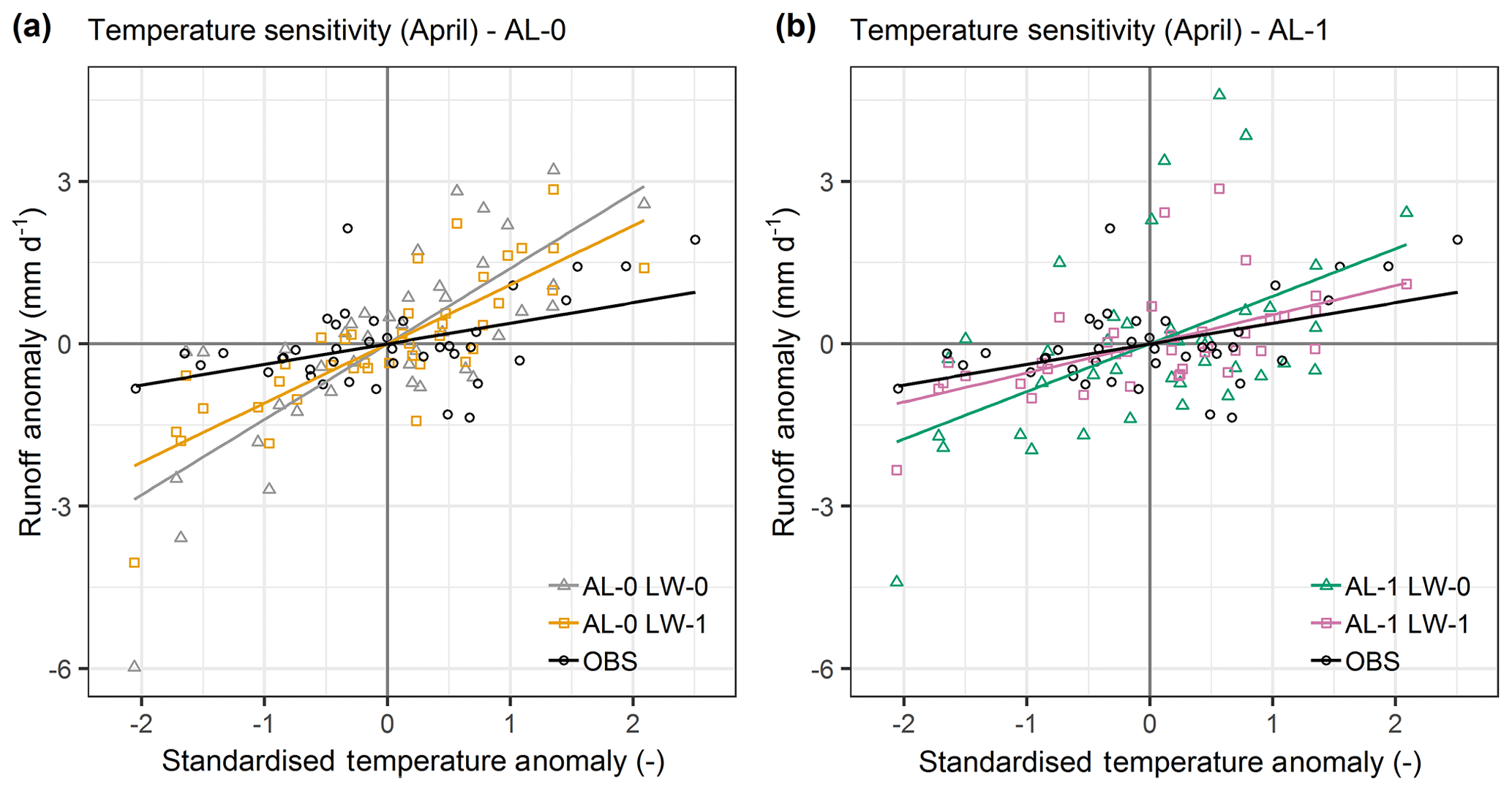
Figure 7Sensitivity of simulated snowpack runoff (and observed total runoff) in April to temperature anomalies for combinations of albedo and liquid water process options (split across two panels for clarity). Points represent 10 d anomalies and lines are from linear regression.
4.5 Climate sensitivity
While simulating specific sequences of climate anomalies and snowpack response is critical for applications such as forecasting, correctly representing the overall sensitivity of snow processes to climate variations and perturbations is crucial for offline and online climate change projections. Given the limitations in the climate input anomaly sequencing identified in Sect. 4.4, this section makes some inferences about the climate sensitivity of FSM configurations on the basis of inter-annual variability. The focus here is on snowpack runoff in the early part of the melt season (April), when snow is typically abundant, such that runoff is primarily constrained by energy rather than mass availability (Sect. 2) and dominated by snowmelt (see also Sects. 3.3, 4.1 and 4.3).
Figure 7 shows the relationship between simulated 10 d air temperature and snowpack runoff anomalies for the four combinations of albedo and liquid water parameterisations. The equivalent relationship using observed temperatures and total runoff is also shown. Figure 7 indicates that the sensitivity of snowpack runoff to climate (temperature) anomalies varies significantly for different model configurations. While scatter in the relationships is notable, likely reflecting the significant influence of other climate variables on the surface energy balance, the relationships are reasonably well approximated by linear regression (all with positive and statistically significant gradients at the 95 % confidence interval). Notably, the shallowest gradient, which is associated with configurations using prognostic albedo and the liquid water parameterisation, agrees best with observations. The consistency of the ranking of the four groups (and observations) can be confirmed with bootstrapping, which shows that 77 % of realisations have the same order as in Fig. 7 (89 %–98 % of realisations if looking at consecutive groups in terms of pairwise rankings). While the multivariate relationships between snow model response and other climate variables could be explored, the example in Fig. 7 demonstrates how fundamental differences in absolute climate sensitivity can be inferred and assessed from (observable) variability.
5.1 Comparison with previous snow model evaluations
Using multiple remote-sensing products to augment sparse local observations, the results in this study support the consensus from previous site-based inter-comparisons that no single snow model configuration performs best in all conditions but that subsets of typically better performing models are identifiable (Essery et al., 2013; Lafaysse et al., 2017; Magnusson et al., 2015). Yet, given both the structural similarity in the FSM ensemble between years and the close ensemble agreement on simulated anomalies, there is a strong indication that errors in the sequencing of climate input anomalies are part of the reason for year-to-year variability in catchment-scale performance in this study. As such, analysing the climate sensitivity of model configurations, based on their responses to historical climate variability, offers a complementary approach to traditional model evaluation methods, especially at scales where climate inputs are subject to large uncertainties. Such an approach could be useful in snow model inter-comparisons such as ESM-SnowMIP (Krinner et al., 2018) as well as for interpreting projections of snow dynamics and their wide-ranging implications in a warming world (e.g. Musselman et al., 2017; Palazzi et al., 2017; Pepin et al., 2015).
In agreement with previous studies, the cold bias in simulated night-time LST provides evidence that turbulent heat fluxes can be overly suppressed under stable atmospheric conditions when using a stability adjustment based on the bulk Richardson number (e.g. Andreadis et al., 2009; Andreas, 2002; Slater et al., 2001). Long-standing and fundamental questions thus remain over the validity of current theories of turbulent exchange under stable conditions, especially in complex terrain. Therefore in future work it would be useful to test alternative or amended stability adjustment options, such as the introduction of a minimum conductance (or maximum flux dampening) parameter (e.g. Collier et al., 2015; Lapo et al., 2019). These tests would ideally be done after adding into FSM other processes omitted in this study that could influence the surface energy balance. These include terrain enhancement of longwave radiation (Sicart et al., 2006), refined treatment of sub-grid variability (Clark et al., 2011), and sensible and latent heat advection (Harder et al., 2017). Although additional processes increase the potential for error compensation, the results in this study reinforce the importance of understanding interactions between snow process parameterisations (e.g. Günther et al., 2019; Lafaysse et al., 2017) and how they vary in time and space.
5.2 Blowing-snow processes and avalanching
Two important influences on snow dynamics in high-mountain catchments are avalanching and blowing-snow processes. The latter includes snow redistribution by wind and associated sublimation during turbulent suspension. In conjunction with orographic precipitation and preferential deposition of snowfall, these processes have been shown to be important for local patterns of snow accumulation and subsequent ablation, especially in high-elevation areas characterised by ridges, crests and steep slopes (e.g. Bernhardt and Schulz, 2010; Grünewald et al., 2010, 2014; MacDonald et al., 2010; Mott et al., 2010, 2014, 2018; Musselman et al., 2015; Strasser et al., 2008; Vionnet et al., 2017).
However, evidence for the influence of these processes at larger scales is mixed. Some studies have suggested that accounting for them leads to improvements in catchment-scale model performance (e.g. Brauchli et al., 2017; Winstral et al., 2013). Yet, when considered together and when larger scales are examined, other results have indicated that these processes may have limited influence on the overall water balance and runoff dynamics (e.g. Bernhardt et al., 2012; Groot Zwaaftink et al., 2013; Vionnet et al., 2014; Warscher et al., 2013). The role of these processes thus appears to depend on the timescales and space scales analysed as well as perhaps the states and fluxes under consideration.
Initial testing showed the overall results of this study to be relatively insensitive to the SnowSlide avalanching parameterisation (Bernhardt and Schulz, 2010). Yet, it is likely that blowing-snow processes need to be considered at the same time to truly capture the relevant interactions (Bernhardt et al., 2012). Therefore not including both avalanching and blowing-snow processes together is a limitation of this study, which focuses instead on the sensitivity of snow cover and runoff dynamics to snowpack process representations. Similar to other mountain regions (e.g. Freudiger et al., 2017), the large mismatch in scale between available HAR climate forcing data and the requirements of blowing-snow simulations makes it difficult to conduct such modelling at present, especially for catchments the size of the Astore. However, very high resolution dynamical downscaling represents a promising avenue to resolve this problem, at least on an event basis (e.g. Bonekamp et al., 2018; Vionnet et al., 2014). This will be an important area for further work.
5.3 Uncertainty in data and parameters
Input data biases and other errors inevitably limit model performance to some extent in such a data-sparse context (Raleigh et al., 2016). However, Sect. S6 in the Supplement indicates that the structure of the ensemble and overall performance variation remain similar if two alternative input strategies are applied (see also Sects. 3.2.3 and S1). Although the distinction of groupings in the ensemble does reduce when using the more observation-based input strategy (Fig. S7 in the Supplement), this may well be the least accurate approach due to the small number of stations available. The results therefore show some robustness to alternative, commonly applied methods for deriving climate input fields in mountain regions for practical applications. Section 4.4 also shows how the larger of the possible input anomaly errors may be identified, which facilitates a better understanding of the occasional performance drops for more physically realistic, typically well performing model configurations (i.e. identification of potential input rather than structural errors, such as underestimation of the warm temperature anomaly in the 2001 ablation season – Sect. 4.4). Further work could attempt a more quantitative uncertainty analysis, but defining meaningful bias ranges and error distributions to test is challenging given currently available local observations.
The FSM parameter defaults appear reasonable for the Astore catchment based on the performance of more physically plausible model configurations across multiple variables in both absolute and normalised and anomaly terms. Further work could undertake calibration and sensitivity analyses, but this would need to guard against overfitting, error compensation and potentially unphysical behaviour given local data limitations, especially for less realistic parameterisations. In any case, recent work suggests that parameter choice in FSM may be of lower importance than both input errors and process parameterisations (Günther et al., 2019).
This study demonstrates that combining local observations, dynamical downscaling and remote-sensing products with multi-physics ensemble frameworks facilitates the identification of skilful process-based snow model configurations in the western Himalaya. Although the importance of different snowpack processes varies with time, space and other model options, the results show that the structure of the FSM ensemble is fundamentally similar between years. Different process parameterisations consistently act to accelerate or delay snowpack runoff and SCA decay. These tendencies lead to notable differences in vertical patterns of snowpack ablation up to very high elevations, with substantial implications for understanding and modelling the evolution of the perennial cryosphere. In agreement with other studies, the results indicate that the prognostic albedo parameterisation should be preferred (Essery et al., 2013; Magnusson et al., 2015). Representation of liquid water retention, refreezing and drainage in the snowpack is also generally required, unless compensatory effects are introduced by other aspects of model configuration, especially the atmospheric stability adjustment option. However, there is evidence that turbulent fluxes are overly suppressed in some conditions by applying the stability adjustment based on the bulk Richardson number implemented in FSM. Correctly simulating these fluxes is a major ongoing challenge in land surface modelling (Lapo et al., 2019), especially in complex terrain.
While no model configuration performs best in all years, the results suggest that errors in climate input anomalies play a key role in this, not just model structural limitations. Model snow cover dynamics and runoff responses to climate variations are more consistent after being transformed to anomalies, which may be useful in forecasting applications, but there is substantial spread within the ensemble in terms of absolute climate sensitivity. This variation in climate sensitivity is critical for model selection in both offline and online simulations supporting climate change impact projections. Together, these points suggest that an ensemble modelling approach should be used in applications where possible. However, a subset of the full FSM ensemble could be taken forward, namely those members which use prognostic albedo and account for snowpack hydrology. Further work could examine input uncertainties in more detail as well as alternative process parameterisations (especially for the stability adjustment), parameter value sensitivity and additional unrepresented processes (such as avalanching and blowing-snow processes). In the complex terrain of the western Himalaya, these tasks would all benefit from higher-resolution dynamical downscaling products to help drive snow models. Advances in these areas could ultimately lead to improved modelling tools to support water resource management in the Himalaya and other mountain regions in a changing climate.
The open-source FSM model code (Essery, 2015) is available here: https://github.com/RichardEssery/FSM (last access: 14 March 2020). An extended version with additional physics and options for multi-site simulations (see Mazzotti et al. 2020) is found at https://github.com/RichardEssery/FSM2 (last access: 14 March 2020). The scripts used to prepare climate inputs and conduct spatially distributed simulations can be requested from the corresponding author.
The HAR data product (Maussion et al. 2014) is publicly available at this site: http://www.klima-ds.tu-berlin.de/har/ (last access: 30 June 2019). MODIS data are also publicly available; instructions for downloading the MODIS products used in this study can be obtained from https://lpdaac.usgs.gov/products/mcd43a3v006/ (last access: 30 June 2019) for MCD43A3 (Schaaf and Wang, 2015), https://lpdaac.usgs.gov/products/mod11a1v006/ (last access: 30 June 2019) for MOD11A1 (Wan et al., 2015) and https://nsidc.org/data/mod10a1 (last access: 30 June 2019) for MOD10A1 (Hall and Riggs, 2016). The observed climate and river flow data sourced from PMD and WAPDA are not currently in a public repository due to data licence restrictions, but these data may be requested from PMD (http://www.pmd.gov.pk/en/, last access: 26 February 2020) and WAPDA (http://www.wapda.gov.pk/, last access: 26 February 2020). In addition, tables summarising the metadata (including coordinates and record periods) and climatology (including long-term averages, annual cycles and variability) for the PMD and WAPDA climate and river flow stations used in this study are available in various publications (e.g. Archer and Fowler, 2004; Archer, 2003; Mukhopadhyay and Khan, 2016; Sharif et al., 2013; Waqas and Athar, 2018). The climate data from the Concordia site run by EvK2CNR can be downloaded from http://share.evk2cnr.org/ (last access: 30 June 2019).
The supplement related to this article is available online at: https://doi.org/10.5194/tc-14-1225-2020-supplement.
With input from NF, GOD, HF and NR, DP designed the study, conducted the modelling and led the analysis. All authors contributed to the interpretation of results. DP drafted the paper, with NF, GOD, HF and NR all providing ideas and alterations.
The authors declare that they have no conflict of interest.
The authors are very grateful to PMD, WAPDA and EvK2CNR for collecting and providing the in situ observations used in this study. We would also sincerely like to thank Fabien Maussion and colleagues for making the HAR dataset publicly available as well as Richard Essery for making the FSM program open-source.
Hayley Fowler was funded by the Wolfson Foundation and the Royal Society through a Royal Society Wolfson Research Merit Award (grant no. WM140025) as well as the European Research Council Grant INTENSE (grant no. ERC-2013-CoG-617329). Nathan Forsythe was supported by the Royal Society (grant nos. CH160148 and CHG/R1/170057) and David Pritchard by an EPSRC doctoral training award (grant no. EP/M506382/1).
This paper was edited by Marie Dumont and reviewed by Matthieu Lafaysse and one anonymous referee.
Andreadis, K. M., Storck, P., and Lettenmaier, D. P.: Modeling snow accumulation and ablation processes in forested environments, Water Resour. Res., 45, W05429, https://doi.org/10.1029/2008WR007042, 2009.
Andreas, E. L.: Parameterizing Scalar Transfer over Snow and Ice: A Review, J. Hydrometeorol., 3, 417–432, https://doi.org/10.1175/1525-7541(2002)003<0417:PSTOSA>2.0.CO;2, 2002.
Archer, D.: Contrasting hydrological regimes in the upper Indus Basin, J. Hydrol., 274, 198–210, https://doi.org/10.1016/S0022-1694(02)00414-6, 2003.
Archer, D. R.: Hydrological implications of spatial and altitudinal variation in temperature in the Upper Indus Basin, Nord. Hydrol., 35, 209–222, https://doi.org/10.2166/nh.2004.0015, 2004.
Archer, D. R. and Fowler, H. J.: Spatial and temporal variations in precipitation in the Upper Indus Basin, global teleconnections and hydrological implications, Hydrol. Earth Syst. Sci., 8, 47–61, https://doi.org/10.5194/hess-8-47-2004, 2004.
Arendt, A., Bliss, A., Bolch, T., Cogley, J. G., Gardner, A. S., Hagen, J.-O., Hock, R., Huss, M., Kaser, G., Kienholz, C., Pfeffer, W. T., Moholdt, G., Paul, F., Radić, V., Andreassen, L., Bajracharya, S., Barrand, N. E., Berthier, E., Bhambri, R., Brown, I., Burgess, E., Burgess, D., Cawkwell, F., Chinn, T., Copland, L., Davies, B., De Angelis, H., Dolgova, E., Earl, L., Filbert, K., Forester, R., Fountain, A. G., Frey, H., Giffen, B., Guo, W. Q., Gurney, S., Hagg, W., Hall, D., Haritashya, U. K., Hartmann, G., Helm, C., Herreid, S., Kapustin, G., Khromova, T., König, M., Kohler, J., Kriegel, D., Kutuzov, S., Lavrentiev, I., Lebris, R., Nosenko, G., Negrete, A., Nuimura, T., Nuth, C., Pettersson, R., Racoviteanu, A., Ranzi, R., Rastner, P., Rau, F., Raup, B., Rich, J., Rott, H., Sakai, A., Schneider, C., Seliverstov, Y., Sharp, M., Sigurðsson, O., Stokes, C., Way, R. G., Wheate, R., Winsvold, S., Wolken, G., Wyatt, F., and Zheltyhina, N.: Randolph Glacier Inventory – A Dataset of Global Glacier Outlines: Version 5.0: Technical Report, Colorado, USA, 2015.
Arino, O., Ramos Perez, J. J., Kalogirou, V., Bontemps, S., Defourny, P., and Van Bogaert, E.: Global Land Cover Map for 2009 (GlobCover 2009), Pangaea, https://doi.org/10.1594/PANGAEA.787668, 2012.
Armstrong, R. L., Rittger, K., Brodzik, M. J., Racoviteanu, A., Barrett, A. P., Khalsa, S.-J. S., Raup, B., Hill, A. F., Khan, A. L., Wilson, A. M., Kayastha, R. B., Fetterer, F., and Armstrong, B.: Runoff from glacier ice and seasonal snow in High Asia: separating melt water sources in river flow, Reg. Environ. Chang., 19, 1249–1261, https://doi.org/10.1007/s10113-018-1429-0, 2019.
Barnett, T. P., Adam, J. C., and Lettenmaier, D. P.: Potential impacts of a warming climate on water availability in snow-dominated regions, Nature, 438, 303–309, https://doi.org/10.1038/nature04141, 2005.
Bernhardt, M. and Schulz, K.: SnowSlide: A simple routine for calculating gravitational snow transport, Geophys. Res. Lett., 37, L11502, https://doi.org/10.1029/2010GL043086, 2010.
Bernhardt, M., Schulz, K., Liston, G. E., and Zängl, G.: The influence of lateral snow redistribution processes on snow melt and sublimation in alpine regions, J. Hydrol., 424–425, 196–206, https://doi.org/10.1016/j.jhydrol.2012.01.001, 2012.
Best, M. J., Pryor, M., Clark, D. B., Rooney, G. G., Essery, R. L. H., Ménard, C. B., Edwards, J. M., Hendry, M. A., Porson, A., Gedney, N., Mercado, L. M., Sitch, S., Blyth, E., Boucher, O., Cox, P. M., Grimmond, C. S. B., and Harding, R. J.: The Joint UK Land Environment Simulator (JULES), model description – Part 1: Energy and water fluxes, Geosci. Model Dev., 4, 677–699, https://doi.org/10.5194/gmd-4-677-2011, 2011.
Biskop, S., Maussion, F., Krause, P., and Fink, M.: Differences in the water-balance components of four lakes in the southern-central Tibetan Plateau, Hydrol. Earth Syst. Sci., 20, 209–225, https://doi.org/10.5194/hess-20-209-2016, 2016.
Bonekamp, P. N. J., Collier, E., and Immerzeel, W. W.: The Impact of Spatial Resolution, Land Use, and Spinup Time on Resolving Spatial Precipitation Patterns in the Himalayas, J. Hydrometeorol., 19, 1565–1581, https://doi.org/10.1175/JHM-D-17-0212.1, 2018.
Brauchli, T., Trujillo, E., Huwald, H., and Lehning, M.: Influence of Slope-Scale Snowmelt on Catchment Response Simulated With the Alpine3D Model, Water Resour. Res., 53, 723–739, https://doi.org/10.1002/2017WR021278, 2017.
Brown, M. E., Racoviteanu, A. E., Tarboton, D. G., Sen Gupta, A., Nigro, J., Policelli, F., Habib, S., Tokay, M., Shrestha, M. S., Bajracharya, S., Hummel, P., Gray, M., Duda, P., Zaitchik, B., Mahat, V., Artan, G., and Tokar, S.: An integrated modeling system for estimating glacier and snow melt driven streamflow from remote sensing and earth system data products in the Himalayas, J. Hydrol., 519, 1859–1869, https://doi.org/10.1016/j.jhydrol.2014.09.050, 2014.
Clark, M. P., Hendrikx, J., Slater, A. G., Kavetski, D., Anderson, B., Cullen, N. J., Kerr, T., Hreinsson, E. Ö., and Woods, R. A.: Representing spatial variability of snow water equivalent in hydrologic and land-surface models: A review, Water Resour. Res., 47, W07539, https://doi.org/10.1029/2011WR010745, 2011.
Clark, M. P., Nijssen, B., Lundquist, J. D., Kavetski, D., Rupp, D. E., Woods, R. A., Freer, J. E., Gutmann, E. D., Wood, A. W., Brekke, L. D., Arnold, J. R., Gochis, D. J., and Rasmussen, R. M.: A unified approach for process-based hydrologic modeling: 1. Modeling concept, Water Resour. Res., 51, 2498–2514, https://doi.org/10.1002/2015WR017200.A, 2015.
Collier, E. and Immerzeel, W. W.: High-resolution modeling of atmospheric dynamics in the Nepalese Himalaya, J. Geophys. Res.-Atmos., 120, 9882–9896, https://doi.org/10.1002/2015JD023266, 2015.
Collier, E., Mölg, T., Maussion, F., Scherer, D., Mayer, C., and Bush, A. B. G.: High-resolution interactive modelling of the mountain glacier–atmosphere interface: an application over the Karakoram, The Cryosphere, 7, 779–795, https://doi.org/10.5194/tc-7-779-2013, 2013.
Collier, E., Maussion, F., Nicholson, L. I., Mölg, T., Immerzeel, W. W., and Bush, A. B. G.: Impact of debris cover on glacier ablation and atmosphere–glacier feedbacks in the Karakoram, The Cryosphere, 9, 1617–1632, https://doi.org/10.5194/tc-9-1617-2015, 2015.
Corripio, J. G.: Vectorial algebra algorithms for calculating terrain parameters from DEMs and solar radiation modelling in mountainous terrain, Int. J. Geogr. Inf. Sci., 17, 1–23, https://doi.org/10.1080/713811744, 2003.
Cox, P. M., Betts, R. A., Bunton, C. B., Essery, R. L. H., Rowntree, P. R., and Smith, J.: The impact of new land surface physics on the GCM simulation of climate and climate sensitivity, Clim. Dynam., 15, 183–203, https://doi.org/10.1007/s003820050276, 1999.
Douville, H., Royer, J.-F., and Mahfouf, J.-F.: A new snow parameterization for the Météo-France climate model. Part I: validation in stand-alone experiments, Clim. Dynam., 12, 21–35, https://doi.org/10.1007/BF00208760, 1995.
Duethmann, D., Zimmer, J., Gafurov, A., Güntner, A., Kriegel, D., Merz, B., and Vorogushyn, S.: Evaluation of areal precipitation estimates based on downscaled reanalysis and station data by hydrological modelling, Hydrol. Earth Syst. Sci., 17, 2415–2434, https://doi.org/10.5194/hess-17-2415-2013, 2013.
Dutra, E., Balsamo, G., Viterbo, P., Miranda, P. M., Beljaars, A., Schär, C., and Elder, K.: An improved snow scheme for the ECMWF land surface model: Description and offline validation, J. Hydrometeorol., 11, 899–916, https://doi.org/10.1175/2010JHM1249.1, 2010.
Essery, R.: Large-scale simulations of snow albedo masking by forests, Geophys. Res. Lett., 40, 5521–5525, https://doi.org/10.1002/grl.51008, 2013.
Essery, R.: A factorial snowpack model (FSM 1.0), Geosci. Model Dev., 8, 3867–3876, https://doi.org/10.5194/gmd-8-3867-2015, 2015.
Essery, R., Rutter, N., Pomeroy, J., Baxter, R., Stähli, M., Gustafsson, D., Barr, A., Bartlett, P., and Elder, K.: SNOWMIP2: An Evaluation of Forest Snow Process Simulations, B. Am. Meteorol. Soc., 90, 1120–1135, doi:https://doi.org/10.1175/2009BAMS2629.1, 2009.
Essery, R., Morin, S., Lejeune, Y., and Ménard, C. B.: A comparison of 1701 snow models using observations from an alpine site, Adv. Water Resour., 55, 131–148, https://doi.org/10.1016/j.advwatres.2012.07.013, 2013.
Etchevers, P., Martin, E., Brown, R., Fierz, C., Lejeune, Y., Bazile, E., Boone, A., Dai, Y., Essery, R., Fernandez, A., Gusev, Y., Jordan, R., Koren, V., Kowalczyk, E., Nasonova, N. O., Pyles, R. D., Schlosser, A., Shmakin, A. B., Smirnova, T. G., Strasser, U., Verseghy, D., Yamazaki, T., and Yang, Z.-L.: Validation of the energy budget of an alpine snowpack simulated by several snow models (SnowMIP project), Ann. Glaciol., 38, 150–158, https://doi.org/10.3189/172756404781814825, 2004.
Finger, D., Pellicciotti, F., Konz, M., Rimkus, S., and Burlando, P.: The value of glacier mass balance, satellite snow cover images, and hourly discharge for improving the performance of a physically based distributed hydrological model, Water Resour. Res., 47, W07519, https://doi.org/10.1029/2010WR009824, 2011.
Forsythe, N., Kilsby, C. G., Fowler, H. J., and Archer, D. R.: Assessment of Runoff Sensitivity in the Upper Indus Basin to Interannual Climate Variability and Potential Change Using MODIS Satellite Data Products, Mt. Res. Dev., 32, 16–29, https://doi.org/10.1659/MRD-JOURNAL-D-11-00027.1, 2012.
Fowler, H. J. and Archer, D. R.: Hydro-climatological variability in the Upper Indus Basin and implications for water resources, in Regional Hydrological Impacts of Climatic Change – Impact Assessment and Decision Making (Proceedings of symposium S6 held during the Seventh IAHS Scientific Assembly at Foz do Iguacu, Brazil, April 2005), IAHS Publ. 295, Foz do Iguacu, Brazil, 2005.
Freudiger, D., Kohn, I., Seibert, J., Stahl, K., and Weiler, M.: Snow redistribution for the hydrological modeling of alpine catchments, WIREs Water, e1232, 1–16, https://doi.org/10.1002/wat2.1232, 2017.
Gafurov, A. and Bárdossy, A.: Cloud removal methodology from MODIS snow cover product, Hydrol. Earth Syst. Sci., 13, 1361–1373, https://doi.org/10.5194/hess-13-1361-2009, 2009.
Groot Zwaaftink, C. D., Mott, R., and Lehning, M.: Seasonal simulation of drifting snow sublimation in Alpine terrain, Water Resour. Res., 49, 1581–1590, https://doi.org/10.1002/wrcr.20137, 2013.
Grünewald, T., Schirmer, M., Mott, R., and Lehning, M.: Spatial and temporal variability of snow depth and ablation rates in a small mountain catchment, The Cryosphere, 4, 215–225, https://doi.org/10.5194/tc-4-215-2010, 2010.
Grünewald, T., Bühler, Y., and Lehning, M.: Elevation dependency of mountain snow depth, The Cryosphere, 8, 2381–2394, https://doi.org/10.5194/tc-8-2381-2014, 2014.
Günther, D., Marke, T., Essery, R., and Strasser, U.: Uncertainties in Snowpack Simulations – Assessing the Impact of Model Structure, Parameter Choice, and Forcing Data Error on Point-Scale Energy Balance Snow Model Performance, Water Resour. Res., 55, 2779–2800, https://doi.org/10.1029/2018WR023403, 2019.
Hall, A. and Qu, X.: Using the current seasonal cycle to constrain snow albedo feedback in future climate change, Geophys. Res. Lett., 33, L03502, https://doi.org/10.1029/2005GL025127, 2006.
Hall, D. K. and Riggs, G. A.: MODIS/Terra Snow Cover Daily L3 Global 500 m Grid, Version 6 (2000–2015), https://doi.org/10.5067/MODIS/MOD10A1.006, 2016.
Harder, P., Pomeroy, J. W., and Helgason, W.: Local-Scale Advection of Sensible and Latent Heat During Snowmelt, Geophys. Res. Lett., 44, 9769–9777, https://doi.org/10.1002/2017GL074394, 2017.
Havens, S., Marks, D., FitzGerald, K., Masarik, M., Flores, A. N., Kormos, P., and Hedrick, A.: Approximating Input Data to a Snowmelt Model Using Weather Research and Forecasting Model Outputs in Lieu of Meteorological Measurements, J. Hydrometeorol., 20, 847–862, https://doi.org/10.1175/JHM-D-18-0146.1, 2019.
Huintjes, E., Sauter, T., Schröter, B., Maussion, F., Yang, W., Kropáček, J., Buchroithner, M., Scherer, D., Kang, S., and Schneider, C.: Evaluation of a coupled snow and energy balance model for Zhadang glacier, Tibetan Plateau, using glaciological measurements and time-lapse photography, Arctic, Antarct. Alp. Res., 47, 573–590, https://doi.org/10.1657/AAAR0014-073, 2015.
Immerzeel, W. W., van Beek, L. P. H., and Bierkens, M. F. P.: Climate Change Will Affect the Asian Water Towers, Science, 382, 1382–1385, https://doi.org/10.1126/science.1183188, 2010.
Jarvis, A., Reuter, H. I., Nelson, A., and Guevara, E.: Hole-filled SRTM for the globe Version 4, available from the CGIAR-CSI SRTM 90 m Database, available at: http://srtm.csi.cgiar.org (last access: 15 March 2016), 2008.
Klemeš, V.: The modelling of mountain hydrology: the ultimate challenge, Hydrol. Mt. Areas, Proceedings of the Strbské Pleso Workshop, Czechoslovakia, June 1988, IAHS 190, 29–44, 1990.
Krinner, G., Derksen, C., Essery, R., Flanner, M., Hagemann, S., Clark, M., Hall, A., Rott, H., Brutel-Vuilmet, C., Kim, H., Ménard, C. B., Mudryk, L., Thackeray, C., Wang, L., Arduini, G., Balsamo, G., Bartlett, P., Boike, J., Boone, A., Chéruy, F., Colin, J., Cuntz, M., Dai, Y., Decharme, B., Derry, J., Ducharne, A., Dutra, E., Fang, X., Fierz, C., Ghattas, J., Gusev, Y., Haverd, V., Kontu, A., Lafaysse, M., Law, R., Lawrence, D., Li, W., Marke, T., Marks, D., Ménégoz, M., Nasonova, O., Nitta, T., Niwano, M., Pomeroy, J., Raleigh, M. S., Schaedler, G., Semenov, V., Smirnova, T. G., Stacke, T., Strasser, U., Svenson, S., Turkov, D., Wang, T., Wever, N., Yuan, H., Zhou, W., and Zhu, D.: ESM-SnowMIP: assessing snow models and quantifying snow-related climate feedbacks, Geosci. Model Dev., 11, 5027–5049, https://doi.org/10.5194/gmd-11-5027-2018, 2018.
Lafaysse, M., Cluzet, B., Dumont, M., Lejeune, Y., Vionnet, V., and Morin, S.: A multiphysical ensemble system of numerical snow modelling, The Cryosphere, 11, 1173–1198, https://doi.org/10.5194/tc-11-1173-2017, 2017.
Lapo, K., Nijssen, B., and Lundquist, J. D.: Evaluation of Turbulence Stability Schemes of Land Models for Stable Conditions, J. Geophys. Res.-Atmos., 124, 3072–3089, https://doi.org/10.1029/2018JD028970, 2019.
Lehning, M., Ingo, V., Gustafsson, D., Nguyen, T. A., Stähli, M., and Zappa, M.: ALPINE3D: a detailed model of mountain surface processes and its application to snow hydrology, Hydrol. Process., 20, 2111–2128, https://doi.org/10.1002/hyp.6204, 2006.
Liston, G. E. and Elder, K.: A Distributed Snow-Evolution Modeling System (SnowModel), J. Hydrometeorol., 7, 1259–1276, https://doi.org/10.1175/JHM548.1, 2006a.
Liston, G. E. and Elder, K.: A Meteorological Distribution System for High-Resolution Terrestrial Modeling (MicroMet), J. Hydrometeorol., 7, 217–234, https://doi.org/10.1175/JHM486.1, 2006b.
Lundquist, J. D., Dettinger, M. D., and Cayan, D. R.: Snow-fed streamflow timing at different basin scales: Case study of the Tuolumne River above Hetch Hetchy, Yosemite, California, Water Resour. Res., 41, W07005, https://doi.org/10.1029/2004WR003933, 2005.
Lute, A. C. and Luce, C. H.: Are Model Transferability and Complexity Antithetical? Insights from Validation of a Variable-Complexity Empirical Snow Model in Space and Time, Water Resour. Res., 53, 8825–8850, https://doi.org/10.1002/2017WR020752, 2017.
Lutz, A. F., Immerzeel, W. W., Shrestha, A. B., and Bierkens, M. F. P.: Consistent increase in High Asia's runoff due to increasing glacier melt and precipitation, Nat. Clim. Change, 4, 587–592, https://doi.org/10.1038/NCLIMATE2237, 2014.
Lutz, A. F., Immerzeel, W. W., Kraaijenbrink, P. D. A., Shrestha, A. B., and Bierkens, M. F. P.: Climate Change Impacts on the Upper Indus Hydrology: Sources, Shifts and Extremes, PLoS One, 11, 1–33, https://doi.org/10.1371/journal.pone.0165630, 2016.
MacDonald, M. K., Pomeroy, J. W., and Pietroniro, A.: On the importance of sublimation to an alpine snow mass balance in the Canadian Rocky Mountains, Hydrol. Earth Syst. Sci., 14, 1401–1415, https://doi.org/10.5194/hess-14-1401-2010, 2010.
Magnusson, J., Wever, N., Essery, R., Helbig, N., Winstral, A., and Jonas, T.: Evaluating snow models with varying process representations for hydrological applications, Water Resour. Res., 51, 2707–2723, https://doi.org/10.1002/2014WR016498, 2015.
Marks, D., Domingo, J., Susong, D., Link, T., and Garen, D.: A spatially distributed energy balance snowmelt model for application in mountain basins, Hydrol. Process., 13, 1935–1959, https://doi.org/10.1002/(SICI)1099-1085(199909)13:12/13<1935::AID-HYP868>3.0.CO;2-C, 1999.
Maussion, F., Scherer, D., Mölg, T., Collier, E., Curio, J., and Finkelnburg, R.: Precipitation Seasonality and Variability over the Tibetan Plateau as Resolved by the High Asia Reanalysis, J. Clim., 27, 1910–1927, https://doi.org/10.1175/JCLI-D-13-00282.1, 2014.
Mazzotti, G., Essery, R., Moeser, C. D., and Jonas, T.: Resolving Small‐Scale Forest Snow Patterns Using an Energy Balance Snow Model With a One‐Layer Canopy, Water Resour. Res., 56, e2019WR026129, https://doi.org/10.1029/2019WR026129, 2020
Moeser, D., Mazzotti, G., Helbig, N., and Jonas, T.: Representing spatial variability of forest snow: Implementation of a new interception model, Water Resour. Res., 52, 1208–1226, https://doi.org/10.1002/2015WR017961, 2016.
Mott, R., Schirmer, M., Bavay, M., Grünewald, T., and Lehning, M.: Understanding snow-transport processes shaping the mountain snow-cover, The Cryosphere, 4, 545–559, https://doi.org/10.5194/tc-4-545-2010, 2010.
Mott, R., Scipión, D., Schneebeli, M., Dawes, N., Berne, A., and Lehning, M.: Orographic effects on snow deposition patterns, J. Geophys. Res.-Atmos., 119, 1419–1439, https://doi.org/10.1002/2013JD019880, 2014.
Mott, R., Vionnet, V., and Grünewald, T.: The Seasonal Snow Cover Dynamics: Review on Wind-Driven Coupling Processes, Front. Earth Sci., 6, 1–25, https://doi.org/10.3389/feart.2018.00197, 2018.
Mukhopadhyay, B. and Khan, A.: Altitudinal variations of temperature, equilibrium line altitude, and accumulation-area ratio in Upper Indus Basin, Hydrol. Res., 48, 214–230, https://doi.org/10.2166/nh.2016.144, 2016.
Musselman, K. N., Pomeroy, J. W., Essery, R. L. H., and Leroux, N.: Impact of windflow calculations on simulations of alpine snow accumulation, redistribution and ablation, Hydrol. Process., 29, 3983–3999, https://doi.org/10.1002/hyp.10595, 2015.
Musselman, K. N., Clark, M. P., Liu, C., Ikeda, K., and Rasmussen, R.: Slower snowmelt in a warmer world, Nat. Clim. Change, 7, 214–220, https://doi.org/10.1038/NCLIMATE3225, 2017.
Naden, P. S.: Spatial variability in flood estimation for large catchments: the exploitation of channel network structure, Hydrol. Sci. J., 37, 53–72, https://doi.org/10.1080/02626669209492561, 1992.
Niu, G. Y., Yang, Z. L., Mitchell, K. E., Chen, F., Ek, M. B., Barlage, M., Kumar, A., Manning, K., Niyogi, D., Rosero, E., Tewari, M., and Xia, Y.: The community Noah land surface model with multiparameterization options (Noah-MP): 1 . Model description and evaluation with local-scale measurements, J. Geophys. Res., 116, D12109, https://doi.org/10.1029/2010JD015139, 2011.
Oleson, K. W., Lawrence, D. M., Bonan, G. B., Drewniak, B., Huang, M., Koven, C. D., Levis, S., Li, F., Riley, W. J., Subin, Z. M., Swenson, S. C., Thornton, P. E., Bozbiyik, A., Fisher, R., Kluzek, E., Lamarque, J.-F., Lawrence, P. J., Leung, L. R., Lipscomb, W., Muszala, S., Ricciuto, D. M., Sacks, W., Sun, Y., Tang, J., and Yang, Z.-L.: Technical Description of version 4.5 of the Community Land Model (CLM), NCAR Technical Note NCAR/TN-503+STR, Boulder, Colorado, USA, 2013.
Palazzi, E., Filippi, L., and Von Hardenberg, J.: Insights into elevation-dependent warming in the Tibetan Plateau-Himalayas from CMIP5 model simulations, Clim. Dynam., 48, 3991–4008, https://doi.org/10.1007/s00382-016-3316-z, 2017.
Pepin, N., Bradley, R., Diaz, H. F., Baraer, M., Caceres, E. B., Forsythe, N., Fowler, H. J., Greenwood, G., Hashmi, M. Z., Liu, X. D., Miller, J. R., Ning, L., Ohmura, A., Palazzi, E., Rangwala, I., Schoener, W., Severskiy, I., Shahgedanova, M., Wang, M. B., Williamson, S. N., and Yang, D. Q.: Elevation-dependent warming in mountain regions of the world, Nat. Clim. Change, 5, 424–430, https://doi.org/10.1038/nclimate2563, 2015.
Prasch, M., Mauser, W., and Weber, M.: Quantifying present and future glacier melt-water contribution to runoff in a central Himalayan river basin, The Cryosphere, 7, 889–904, https://doi.org/10.5194/tc-7-889-2013, 2013.
Pritchard, D. M. W., Forsythe, N., Fowler, H. J., O'Donnell, G. M., and Li, X.-F.: Evaluation of Upper Indus Near-Surface Climate Representation by WRF in the High Asia Refined Analysis, J. Hydrometeorol., 20, 467–487, https://doi.org/10.1175/JHM-D-18-0030.1, 2019.
Quéno, L., Vionnet, V., Dombrowski-Etchevers, I., Lafaysse, M., Dumont, M., and Karbou, F.: Snowpack modelling in the Pyrenees driven by kilometric-resolution meteorological forecasts, The Cryosphere, 10, 1571–1589, https://doi.org/10.5194/tc-10-1571-2016, 2016.
Ragettli, S., Pellicciotti, F., Bordoy, R., and Immerzeel, W. W.: Sources of uncertainty in modeling the glaciohydrological response of a Karakoram watershed to climate change, Water Resour. Res., 49, 6048–6066, https://doi.org/10.1002/wrcr.20450, 2013.
Ragettli, S., Pellicciotti, F., Immerzeel, W. W., Miles, E. S., Petersen, L., Heynen, M., Shea, J. M., Stumm, D., Joshi, S., and Shrestha, A.: Unraveling the hydrology of a Himalayan catchment through integration of high resolution in situ data and remote sensing with an advanced simulation model, Adv. Water Resour., 78, 94–111, https://doi.org/10.1016/j.advwatres.2015.01.013, 2015.
Raleigh, M. S., Lundquist, J. D., and Clark, M. P.: Exploring the impact of forcing error characteristics on physically based snow simulations within a global sensitivity analysis framework, Hydrol. Earth Syst. Sci., 19, 3153–3179, https://doi.org/10.5194/hess-19-3153-2015, 2015.
Raleigh, M. S., Livneh, B., Lapo, K., and Lundquist, J. D.: How Does Availability of Meteorological Forcing Data Impact Physically Based Snowpack Simulations?, J. Hydrometeorol., 17, 99–120, https://doi.org/10.1175/JHM-D-14-0235.1, 2016.
Revuelto, J., Lafaysse, M., Zin, I., Charrois, L., Vionnet, V., Dumont, M., Rabatel, A., Six, D., Condom, T., Morin, S., Viani, A., and Sirguey, P.: Multi-Criteria Evaluation of Snowpack Simulations in Complex Alpine Terrain Using Satellite and In Situ Observations, Remote Sens., 10, 1–32, https://doi.org/10.3390/rs10081171, 2018.
Rutter, N., Essery, R., Pomeroy, J., Altimir, N., Andreadis, K., Baker, I., Barr, A., Bartlett, P., Boone, A., Deng, H., Douville, H., Dutra, E., Elder, K., Ellis, C., Feng, X., Gelfan, A., Goodbody, A., Gusev, Y., Gustafsson, D., Hellström, R., Hirabayashi, Y., Hirota, T., Jonas, T., Koren, V., Kuragina, A., Lettenmaier, D., Li, W., Luce, C., Martin, E., Nasonova, O., Pumpanen, J., Pyles, R. D., Samuelsson, P., Sandells, M., Schädler, G., Shmakin, A., Smirnova, T. G., Stähli, M., Stöckli, R., Strasser, U., Su, H., Suzuki, K., Takata, K., Tanaka, K., Thompson, E., Vesala, T., Viterbo, P., Wiltshire, A., Xia, K., Xue, Y., and Yamazaki, T.: Evaluation of forest snow processes models (SnowMIP2), J. Geophys. Res., 114, D06111, https://doi.org/10.1029/2008JD011063, 2009.
Salomonson, V. V and Appel, I.: Estimating fractional snow cover from MODIS using the normalized difference snow index, Remote Sens. Environ., 89, 351–360, https://doi.org/10.1016/j.rse.2003.10.016, 2004.
Schaaf, C. and Z. Wang. MCD43A3 MODIS/Terra+Aqua BRDF/Albedo Daily L3 Global – 500 m V006, distributed by NASA EOSDIS Land Processes DAAC, https://doi.org/10.5067/MODIS/MCD43A3.006, 2015.
Shakoor, A. and Ejaz, N.: Flow Analysis at the Snow Covered High Altitude Catchment via Distributed Energy Balance Modeling, Sci. Rep., 9, 1–14, https://doi.org/10.1038/s41598-019-39446-1, 2019.
Sharif, M., Archer, D. R., Fowler, H. J., and Forsythe, N.: Trends in timing and magnitude of flow in the Upper Indus Basin, Hydrol. Earth Syst. Sci., 17, 1503–1516, https://doi.org/10.5194/hess-17-1503-2013, 2013.
Shrestha, M., Koike, T., Hirabayashi, Y., Xue, Y., Wang, L., Rasul, G., and Ahmad, B.: Integrated simulation of snow and glacier melt in water and energy balance-based, distributed hydrological modeling framework at Hunza River Basin of Pakistan Karakoram region, J. Geophys. Res.-Atmos., 120, 4889–4919, https://doi.org/10.1002/2014JD022666, 2015.
Sicart, J. E., Pomeroy, J. W., Essery, R. L. H., and Bewley, D.: Incoming longwave radiation to melting snow: observations, sensitivity and estimation in northern environments, Hydrol. Process., 20, 3697–3708, https://doi.org/10.1002/hyp.6383, 2006.
Skamarock, W. C., Klemp, J. B., Dudhia, J., Gill, D. O., Barker, D. M., Duda, M. G., Huang, X.-Y., Wang, W., and Power, J. G.: A Description of the Advanced Research WRF Version 3, NCAR Technical Note NCAR/TN–475+STR, 2008.
Slater, A. G., Schlosser, C. A., Desborough, C. E., Pitman, A. J., Henderson-Sellers, A., Robock, A., Vinnikov, K. Y., Mitchell, K., Boone, A., Braden, H., Chen, F., Cox, P. M., de Rosnay, P., Dickinson, R. E., Dai, Y.-J., Duan, Q., Entin, J., Etchevers, P., Gedney, N., Gusev, Y. M., Kim, J., Koren, V., Kowalczyk, E. A., Nasonova, O. N., Noilhan, J., Schaake, S., Shmakin, A. B., Smirnova, T. G., Verseghy, D., Wetzel, P., Xue, Y., Yang, Z.-L., and Zeng, Q.: The Representation of Snow in Land Surface Schemes: Results from PILPS 2 (d), J. Hydrometeorol., 2, 7–25, https://doi.org/10.1175/1525-7541(2001)002<0007:TROSIL>2.0.CO;2, 2001.
Stigter, E. E., Wanders, N., Saloranta, T. M., Shea, J. M., Bierkens, M. F. P., and Immerzeel, W. W.: Assimilation of snow cover and snow depth into a snow model to estimate snow water equivalent and snowmelt runoff in a Himalayan catchment, The Cryosphere, 11, 1647–1664, https://doi.org/10.5194/tc-11-1647-2017, 2017.
Strasser, U., Bernhardt, M., Weber, M., Liston, G. E., and Mauser, W.: Is snow sublimation important in the alpine water balance?, The Cryosphere, 2, 53–66, https://doi.org/10.5194/tc-2-53-2008, 2008.
Tarasova, L., Knoche, M., Dietrich, J., and Merz, R.: Effects of input discretization, model complexity, and calibration strategy on model performance in a data-scarce glacierized catchment in Central Asia, Water Resour. Res., 52, 4674–4699, https://doi.org/10.1002/2015WR018551, 2016.
Verseghy, D. L.: CLASS – A Canadian land surface scheme for GCMs. I. Soil model, Int. J. Climatol., 11, 111–133, https://doi.org/10.1002/joc.3370110202, 1991.
Vionnet, V., Brun, E., Morin, S., Boone, A., Faroux, S., Le Moigne, P., Martin, E., and Willemet, J.-M.: The detailed snowpack scheme Crocus and its implementation in SURFEX v7.2, Geosci. Model Dev., 5, 773–791, https://doi.org/10.5194/gmd-5-773-2012, 2012.
Vionnet, V., Martin, E., Masson, V., Guyomarc'h, G., Naaim-Bouvet, F., Prokop, A., Durand, Y., and Lac, C.: Simulation of wind-induced snow transport and sublimation in alpine terrain using a fully coupled snowpack/atmosphere model, The Cryosphere, 8, 395–415, https://doi.org/10.5194/tc-8-395-2014, 2014.
Vionnet, V., Martin, E., Masson, V., Lac, C., Bouvet, F. N., and Guyomarc'h, G.: High-Resolution Large Eddy Simulation of Snow Accumulation in Alpine Terrain, J. Geophys. Res.-Atmos., 122, 11005–11021, https://doi.org/10.1002/2017JD026947, 2017.
Viviroli, D., Archer, D. R., Buytaert, W., Fowler, H. J., Greenwood, G. B., Hamlet, A. F., Huang, Y., Koboltschnig, G., Litaor, M. I., López-Moreno, J. I., Lorentz, S., Schädler, B., Schreier, H., Schwaiger, K., Vuille, M., and Woods, R.: Climate change and mountain water resources: overview and recommendations for research, management and policy, Hydrol. Earth Syst. Sci., 15, 471–504, https://doi.org/10.5194/hess-15-471-2011, 2011.
Wan, Z.: New refinements and validation of the collection-6 MODIS land-surface temperature/emissivity product, Remote Sens. Environ., 140, 36–45, https://doi.org/10.1016/j.rse.2013.08.027, 2014.
Wan, Z., Zhang, Y., Zhang, Q., and Li, Z.-L.: Quality assessment and validation of the MODIS global land surface temperature, Int. J. Remote Sens., 25, 261–274, https://doi.org/10.1080/0143116031000116417, 2004.
Wan, Z., Hook, S., and Hulley, G.: MOD11A1 MODIS/Terra Land Surface Temperature/Emissivity Daily L3 Global 1 km SIN Grid V006, distributed by NASA EOSDIS Land Processes DAAC, https://doi.org/10.5067/MODIS/MOD11A1.006, 2015
Waqas, A. and Athar, H.: Observed diurnal temperature range variations and its association with observed cloud cover in northern Pakistan, Int. J. Climatol., 38, 3323–3336, https://doi.org/10.1002/joc.5503, 2018.
Warscher, M., Strasser, U., Kraller, G., Marke, T., Franz, H., and Kunstmann, H.: Performance of complex snow cover descriptions in a distributed hydrological model system: A case study for the high Alpine terrain of the Berchtesgaden Alps, Water Resour. Res., 49, 2619–2637, https://doi.org/10.1002/wrcr.20219, 2013.
Winstral, A., Marks, D., and Gurney, R.: Simulating wind-affected snow accumulations at catchment to basin scales, Adv. Water Resour., 55, 64–79, https://doi.org/10.1016/j.advwatres.2012.08.011, 2013.