Using 3D turbulence-resolving simulations to understand the impact of surface properties on the energy balance of a debris-covered glacier

Bonekamp, Pleun N. J.; van Heerwaarden, Chiel C.; Steiner, Jakob F.; Immerzeel, Walter W.

doi:https://doi.org/10.5194/tc-14-1611-2020

Articles | Volume 14, issue 5

https://doi.org/10.5194/tc-14-1611-2020

Articles | Volume 14, issue 5

Research article

26 May 2020

Research article |

| 26 May 2020

Using 3D turbulence-resolving simulations to understand the impact of surface properties on the energy balance of a debris-covered glacier

Pleun N. J. Bonekamp, Chiel C. van Heerwaarden, Jakob F. Steiner, and Walter W. Immerzeel

Abstract

Debris-covered glaciers account for almost one-fifth of the total glacier ice volume in High Mountain Asia; however, their contribution to the total glacier melt remains uncertain, and the drivers controlling this melt are still largely unknown. Debris influences the properties (e.g. albedo, thermal conductivity, roughness) of the glacier surface and thus the surface energy balance and glacier melt. In this study we have used sensitivity tests to assess the effect of surface properties of debris on the spatial distribution of micrometeorological variables such as wind fields, moisture and temperature. Subsequently we investigated how those surface properties drive the turbulent fluxes and eventually the conductive heat flux of a debris-covered glacier.

We simulated a debris-covered glacier (Lirung Glacier, Nepal) at a 1 m resolution with the MicroHH model, with boundary conditions retrieved from an automatic weather station (temperature, wind and specific humidity) and unmanned aerial vehicle flights (digital elevation map and surface temperature). The model was validated using eddy covariance data. A sensitivity analysis was then performed to provide insight into how heterogeneous surface variables control the glacier microclimate. Additionally, we show that ice cliffs are local melt hot spots and that turbulent fluxes and local heat advection amplify spatial heterogeneity on the surface. The high spatial variability of small-scale meteorological variables suggests that point-based station observations cannot be simply extrapolated to an entire glacier. These outcomes should be considered in future studies for a better estimation of glacier melt in High Mountain Asia.

How to cite

How to cite.

Dates

Received: 23 Oct 2019 – Discussion started: 06 Nov 2019 – Revised: 06 Apr 2020 – Accepted: 21 Apr 2020 – Published: 26 May 2020

1 Introduction

Glaciers in High Mountain Asia (HMA) act as a fresh water supply for millions of people living downstream, and this supply will change due to global warming (Lutz et al., 2013; Wester et al., 2019). Debris-covered glaciers account for 18 % of the total glacier ice volume in High Mountain Asia; however, the exact melt processes of these glaciers are still unknown, and their contribution to the total glacier melt remains uncertain (Kraaijenbrink et al., 2017).

Debris-covered glacier surfaces differ from clean-ice glaciers – with surface temperatures that can exceed the melting point considerably, a higher topographic variability and the possibility of an unsaturated surface. Debris influences the surface energy balance and therefore glacier melt by influencing the properties (e.g. albedo, thermal conductivity) of the glacier surface (Reid and Brock, 2010). Due to the albedo effect glacier ablation is generally enhanced by debris thickness smaller than a few centimetres, while it decreases exponentially with thickening debris due to ice insulation (Östrem, 1959).

The energy exchange between the (debris-covered) glacier surface and atmosphere is determined by small-scale meteorological conditions rather than large-scale weather patterns (Sauter and Galos, 2016). Heterogeneous surface conditions affect the microclimate, resulting in large spatial differences in energy balance components (Reid and Brock, 2010). For example, daytime surface temperatures can range between melting point (ice and water) and 27.5 ^∘C due to inhomogeneous surface heating and variable debris thickness (Kraaijenbrink et al., 2018; Steiner and Pellicciotti, 2016), and the surface roughness length ranges from ∼ 0.005 m (gravel) to ∼ 0.5 m (boulders; Miles et al., 2017a). Local melt hot spots generally exist on the surface of a debris-covered glacier in the form of ice cliffs and supraglacial ponds (Buri et al., 2016a; Miles et al., 2016), causing highly heterogeneous ablation rates. However, it is not entirely understood how those ice cliffs and ponds form, evolve and disappear. While the cut and closure of englacial drainage systems is likely to be an important driver (Benn et al., 2017; Miles et al., 2017b), and the interaction between cliffs and ponds is an important process (Miles et al., 2017b; Steiner et al., 2019), heterogeneous meteorological forcing over the debris surface may also play a major role (Buri and Pellicciotti, 2018). The influence of spatial variability and especially with respect to turbulent exchange in the atmosphere has, however, not previously been investigated.

Currently there are several methods to model the melt of a debris-covered glacier spatially, including a multilayer energy balance model (Fyffe et al., 2014; Reid and Brock, 2010) as well as specifically for surface features on debris cover (Buri et al., 2016b; Miles et al., 2018) and a fully coupled atmosphere–glacier mass balance model (Collier et al., 2013), with the latter including two-way debris–atmosphere feedbacks. However these approaches remain limited in their scope as they cannot adequately address the spatial and temporal distribution of surface and meteorological variables. This is because atmospheric field observations on debris-covered tongues are limited to only a few field locations in the Himalaya (Lejeune et al., 2013; Ragettli et al., 2013; Rounce et al., 2015; Steiner et al., 2018), the Karakoram (Mihalcea et al., 2008) and the Tien Shan (Yao et al., 2014). All of these studies cover relatively short time spans ranging from days to multiple months. Extrapolating point measurements remains a challenge when it comes to debris-covered glaciers, as measurements from a single weather station are not representative of the complex, inhomogeneous terrain. In a situation where there is large spatial variation, a high-resolution modelling approach can give important new insights into the coupling and interaction between the surface and the atmosphere (Mott et al., 2014).

Turbulent fluxes can play a substantial role in the surface energy balance of debris-covered glaciers (Rounce et al., 2015; Steiner et al., 2018). These fluxes are often calculated using the bulk method, where the sensible and latent heat fluxes are related to the temperature and moisture gradients between the atmosphere and surface respectively. However, the bulk method assumes atmospheric stability and a constant surface roughness, which is not valid over debris-covered glacier surfaces (Steiner et al., 2018). Steiner et al. (2018) found, for example, that bulk methods overestimate turbulent heat fluxes.

High-resolution turbulence-resolving simulations offer a means of gaining insight into the microclimate of a debris-covered glacier (i.e. wind, humidity and temperature fields). Turbulence can be simulated by two techniques: LES (large eddy simulation) and DNS (direct numerical simulation). The difference between these simulations is the treatment of the smallest scales in the flow; LES uses a sub-grid parameterization while DNS resolves these explicitly. DNS at atmospheric viscosity is computationally unfeasible. It is, however, not always necessary to resolve all scales, as many flow characteristics become independent of the Reynolds number at much larger values for the viscosity than that of the atmosphere. In this paper, we build on this property (see Appendix A). One could also refer to this approach as “LES with a constant eddy viscosity”.

Large-eddy simulations (LES) studies have been conducted for clean-ice glaciers, focussing on katabatic winds and sensible heat fluxes (e.g. Axelsen and van Dop 2009a, b; Sauter and Galos, 2016). LES often implies a simplification of reality, such as a flat terrain and horizontally homogeneous meteorological conditions (Axelsen and van Dop, 2009a), though simulations can give insight into fundamental processes. LES ignores the smallest length scales of turbulence and can be used if the behaviour of those scales can be described as a function of the resolved structures in the simulation. In order to also resolve the smallest length scales, direct numerical simulation (DNS) should be used.

Both DNS and LES have advantages and drawbacks for the simulation of atmospheric turbulent flows. Generally, it is assumed LES represents high Reynolds numbers well, while DNS is only correct if all scales in the flow are resolved. However, as shown by Moin and Mahesh (1998), it is in many cases unnecessary to resolve the flow up to the Kolmogorov scale, as many of the statistics of turbulent flows become independent of the Reynolds number at Reynolds numbers far less than the atmospheric Reynolds number. This is proven for convective boundary layers in the atmosphere (van Heerwaarden and Mellado, 2016), turbulent channel flow (e.g. Moser et al., 1999; Schultz and Flack, 2013), Ekman flow (Spalart, 2009) and stable atmospheric boundary layers (Ansorge and Mellado, 2016). Additionally, Dimotakis (2000) has delivered clear guidelines on estimating whether turbulence is fully developed. We are converging to that situation in this study as we show that only a marginal part of the total variance is missed and the most relevant results are independent of the Reynolds number.

Applying LES combined with wall models in complex terrain is questionable. The Monin–Obukhov similarity theory (MOST) that is used to compute the interaction with the wall has already been demonstrated invalid over simple slopes (Nadeau et al., 2013). Wall modelling on the faces of non-horizontal objects is an unsolved challenge, as all assumptions of the MOST break down. With no alternative is available, MOST is often used nonetheless. The consequences of this are potentially harder to estimate and interpret than those of moderate Reynolds numbers in the application of DNS.

The drivers of heterogeneous melt patterns on debris-covered glaciers, and the role turbulent fluxes play, are not well understood. In this study the impact of surface properties (roughness, surface temperature and surface moisture) of debris on the spatial distribution of small-scale meteorological variables, such as wind fields, moisture and temperature, and subsequently the turbulent fluxes and conductive heat flux, is investigated for the Lirung Glacier (Nepal) using a DNS model with constant eddy viscosity and a spatial resolution of ∼ 1 m. Observational data are used as boundary conditions, which include a high-resolution DEM (digital elevation map) and thermal imagery, retrieved from UAV (unmanned aerial vehicle) flights. We show the impact of heterogeneous surface conditions, and we show that turbulent fluxes are an important contributor to the energy balance of ice cliffs. This is the first high-resolution study for a debris-covered glacier that investigates the effects of debris on meteorological variables using a turbulent fluxes resolving model. This study improves our understanding of the processes of debris-glacier melt and will lead to a better understanding of the contribution of debris-glacier melt to current river discharges, as well as how this will change in future.

2 Methods

2.1 Study area

Lirung Glacier is a debris-covered glacier in the Langtang catchment located 50 km north of Kathmandu (Nepal; Fig. 1). The Langtang catchment has an area of approximately 560 km², of which 30 % is glacierized. One-fourth of all the Langtang glaciers are debris covered. Lirung Glacier itself is 3.5 km long and on average 500 m wide (Immerzeel et al., 2014a) and ranges in elevation from 4000 to 7132 m a.s.l. The surface is highly heterogeneous and debris is composed of a range of textures from silt to gravel to boulders (Miles et al., 2017a). The average gradient of the tongue is approximately 2 ^∘C, and debris thickness ranges from 0.1 to 2.0 m (McCarthy et al., 2017). This area is influenced during the summer months by the Indian summer monsoon, which provides 70 % of the annual precipitation (Immerzeel et al., 2014b). The winters are relatively dry and precipitation generally occurs only during a few cyclonic events (Bonekamp et al., 2019a; Collier and Immerzeel, 2015).

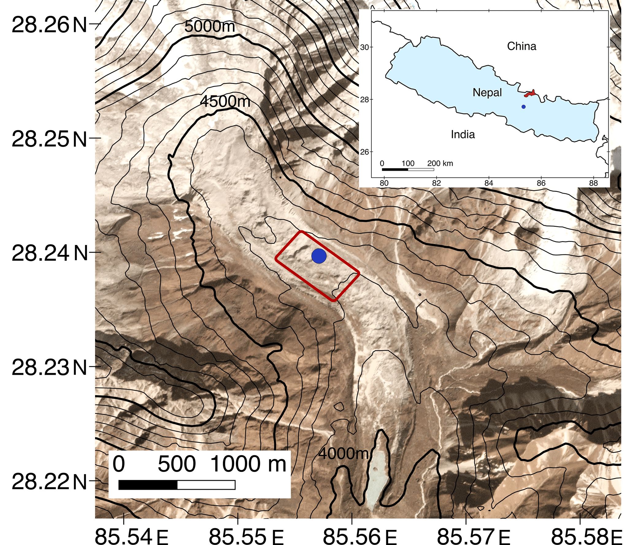
https://www.the-cryosphere.net/14/1611/2020/tc-14-1611-2020-f01

Figure 1Lirung Glacier with the MicroHH domain (red contour) and the location of the AWS (blue point). The background image is a Planet image from 9 December 2018 (Planet Team, 2017). The inset shows the Langtang catchment (red) and its location in Nepal.

2.2 Field measurements

Automatic weather station (AWS) data on the glacier (Fig. 1) is used for model validation (air temperature, wind speed, relative humidity, and incoming and outgoing short- and longwave radiation). For this study we only use the measurements between 10:30 and 11:30 LT on 12 October 2016 (10 min average; Steiner et al., 2018). The sensible and latent heat fluxes are derived from high-frequency measurements (10 Hz) of fluctuations in temperature, humidity and wind speed with the IRGASON eddy covariance (EC) system (5 min average). The footprint of the EC system depends on its sensor orientation, wind speed and direction (Steiner et al., 2018) and complicates the direct comparison between measurements and simulation. We used the footprint as described in Steiner et al. (2018) and determined the weighted contribution of each model pixel within the footprint area to the flux observation at the AWS site to ensure a fair comparison with the measurements.

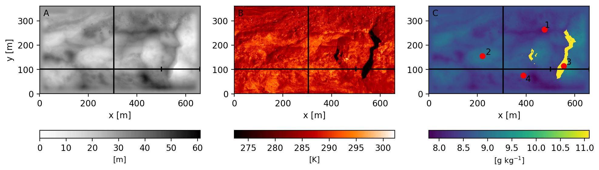
https://www.the-cryosphere.net/14/1611/2020/tc-14-1611-2020-f02

Figure 2Boundary conditions used in MicroHH: the DEM (a), surface temperature (b) and surface specific humidity (c). Black lines (a–c) indicate the locations of the vertical cross sections used in Figs. 5–7. The vertical cross section used in Fig. 9 is a subset of the cross section (x=500–660, y=102). Its start and end points are indicated by small vertical lines. Red points indicate the locations used in Fig. 8 (1: dry debris; 2: wet debris; 3: ice cliff; 4: AWS).

Download

The high-resolution DEM is based on the structure-from-motion workflow using optical imagery retrieved on 9 October 2016 (13:00 LT) and resampled to 1 m resolution for further use (Fig. 2a) (Immerzeel et al., 2014a; Kraaijenbrink et al., 2016). A resolution of 1 m is the highest possible spatial resolution we could achieve given the constraints of computational power and input data. In Appendix A we show that the spatial resolution of 1 m is sufficient to capture the characteristics of the flow and that increasing the resolution will not improve the information derived. The surface temperature (12 October 2016, 11:00 LT) was retrieved with the UAV thermal infrared camera and is bias corrected (Kraaijenbrink et al., 2018). We use only a subset of the UAV data in this research, since the domain is constrained by the intersect of the optical and thermal flight extent, and the domain should be rectangular in the model. The DEM of the domain is detrended, rotated to the main wind direction and smoothed at the boundaries in order to connect the outer left pixels with the outer right pixels of the domain to allow for periodic boundaries. Periodic boundary conditions presume that the fluxes exiting the domain are used as influx in the next time step. This allows us to investigate processes and feedbacks solely in the domain, as larger forcings are excluded. We include only the glacier surface in the domain and not the surrounding moraines. The final extent of the domain is 660 m×361 m the final detrended topography ranges from 0 to 57 m, and the surface temperature ranges from 273.1 K (ice cliff at melting point) to 302.2 K with an average of 282.2 K. The corresponding potential temperature is 331.3 K. In total 2 % of the domain is covered with ice cliffs and is representative for glaciers in the Langtang catchment as the ice cliff glacier average is found to be between 1.4 % and 3.4 % (Steiner et al., 2019).

2.3 Model

The MicroHH model (van Heerwaarden et al., 2017) is a computational fluid dynamics model designed to simulate turbulent flows in the atmosphere through direct numerical simulation (DNS) and large eddy simulation (LES). We use MicroHH as a DNS model with a constant eddy viscosity, which effectively renders a LES with the most primitive eddy viscosity model possible. MicroHH can be run in parallel and is made for efficient computations. The configuration of the model makes allowance for heterogeneous surface boundary conditions such as topography, surface temperature and surface specific humidity. We give a brief description of the model below. More detail can be found in van Heerwaarden et al. (2017).

MicroHH solves the conservation equations of mass, momentum and energy under the Boussinesq approximation. The model assumes constant density with altitude, thus simplifying the governing equations substantially. The conservation of mass is thereby reduced to the conservation of volume in Einstein summation:

\begin{matrix} (1) & \frac{\partial u_{i}}{\partial x_{i}} = 0 . \end{matrix}

u_i represents components of the velocity vector (u, v, w) and x_i is the position of the vector (x, y, z). The thermodynamics are a relation between fluctuations of virtual potential temperature ( ${ϑ^{'}}_{v}$ ) and density (ρ^′) under the Boussinesq approximation by

\begin{matrix} (2) & \frac{{ϑ^{'}}_{v}}{ϑ_{v 0}} = - \frac{ρ^{'}}{ρ_{0}}, \end{matrix}

with ϑ_v0 the reference virtual potential temperature and ρ₀ the reference density. The conservation of momentum is formulated as

\begin{matrix} (3) & \frac{\partial u_{i}}{\partial t} = - \frac{\partial u_{i} u_{j}}{\partial x_{j}} - \frac{1}{ρ_{0}} \frac{\partial p^{'}}{\partial x_{i}} + δ_{i 3} g \frac{{θ^{'}}_{v}}{θ_{v 0}} + ν \frac{\partial^{2} u_{i}}{\partial x_{j}^{2}} + F_{i}, \end{matrix}

where δ is the Kronecker delta, ν the kinematic viscosity, g the gravity constant (9.81 m s⁻²) and F_i the external forces originating from, for example, large-scale forcings. We used moist dynamics in our simulations, and this implies that the liquid water potential temperature θ_l is the conserved variable in the energy conservation equation.

\begin{matrix} (4) & θ_{l} \approx θ - \frac{L_{v}}{c_{p} Π} q_{l}, \end{matrix}

with L_v the latent heat of vaporization (2.5×10⁶ kJ kg⁻¹), c_p the specific heat of dry air (1002 kJ kg⁻¹), q_l the cloud liquid water specific humidity and Π the Exner function:

\begin{matrix} (5) & Π = {(\frac{p}{p_{00}})}^{R_{d} / c_{p}}, \end{matrix}

with p the actual pressure, p₀₀ the reference pressure (1000 hPa) and R_d the gas constant for dry air (287.058 J kg⁻¹ K⁻¹).

The conservation of energy is defined by

\begin{matrix} (6) & \frac{\partial θ_{l}}{\partial t} = - \frac{1}{ρ_{0}} \frac{\partial ρ_{0 u_{j}} θ_{l}}{\partial x_{j}} + κ_{θ} \frac{\partial^{2} θ_{l}}{\partial x_{j}^{2}} + \frac{θ_{l 0}}{ρ_{0} c_{p} T_{0}} Q . \end{matrix}

The density of dry air (ρ₀) is measured via the eddy covariance system and is set to 0.75 kg m⁻³, κ_θ is the thermal diffusivity for heat and chosen commensurate with the Reynolds number in order to stay close to the Prandtl number of the atmosphere (Sect. 2.4), and Q is the external heat source or sink. T₀ is the reference temperature profile.

MicroHH provides output of the 3D variables (total specific moisture, liquid potential temperature, and the u and v components of the wind) at desired cross sections parallel along the axes x, y, z. The accumulated temperature (thl_flux) and moisture fluxes (qt_flux) are given at the surface of a grid cell and should be divided by the surface area of that cell to obtain the flux in watts per square metre (W m⁻²). Therefore, the fluxes are converted to a sensible heat flux (SHF) and latent heat flux (LHF) by

\begin{matrix} (7) & SHF = ρ \cdot {thl}_{flux} \cdot c_{p} \end{matrix}

and

\begin{matrix} (8) & LHF = ρ \cdot {qt}_{flux} \cdot L_{v}, \end{matrix}

where thl_flux and qt_flux are the diffusive fluxes perpendicular to the surface and are directly dependent on the temperature and moisture gradient between the surface and the atmosphere.

2.4 Boundary conditions

The bottom boundary condition for the velocity components is set to a Dirichlet no-slip condition (zero velocity at this interface) and the top boundary condition is a Neumann free-slip condition (velocity gradient). Random noise is added to the flow in order to add turbulence and is applied to the wind vectors u and v with an amplitude of 0.1 m s⁻¹. Preferably, the viscosity of the atmosphere is used in the simulations; however, this is not computationally feasible in our simulations. Therefore, we chose the lowest possible eddy viscosity and checked the results for convergence (Sect. 4). The Prandtl number (ν∕κ_θ, 2 and 1.2 for the two Reynolds numbers) is chosen such that it remains close to the value of the atmosphere (0.71). This approach follows earlier direct numerical simulation studies of the atmosphere (e.g. Van Heerwaarden et al., 2014; Mellado, 2012). In the vicinity of unity, the flow characteristics are insensitive to the exact value of the Prandtl number (Ahlers et al., 2009). A second-order spatial discretization scheme is used. A buffer zone of the upper 100 m is used for numerical stability, and the state values decrease exponentially to the top boundary. The boundary conditions at the DEM surface are Dirichlet boundary conditions and can be prescribed spatially for specific humidity and surface temperature. In our experiments the surface temperature is set to values measured by the UAV. The specific humidity is not measured spatially by the UAV, although the spatial variability of the relative humidity (RH) is made dependent on the topography to indicate dry higher-elevated areas and wetter depressions by

\begin{matrix} (9) & RH = {RH}_{0} - 0.26 \cdot DEM, \end{matrix}

with RH₀=85 % at the lowest point and RH = 70 % at the highest point of the DEM – and an average of q=8.6 g kg⁻¹. This approximation follows the reasoning that meltwater entrained in the debris accumulates in depressions. Additionally, finer-grained debris from washouts tends to be found in depressions, resulting in a higher surface retention capacity. At the site location of the AWS the relative humidity (measured at 3.1 m) is 66 %, and with this relationship we assume the surface is moister than the atmosphere everywhere. The relative humidity at the AWS location during the morning varied from 54 % to 100 % over time, which is typical of general diurnal variability (Steiner et al., 2018). We assume a spatially constant saturation vapour pressure in the domain, based on the air temperature measured by the AWS. Using Tetens' formula,

\begin{matrix} (10) & e_{s} = 0.61078 \cdot e^{\frac{17.27 \cdot T}{(T + 237.3)}}, \end{matrix}

we calculated the spatial variable specific humidity as

\begin{matrix} (11) & q = \frac{RH}{100 %} \cdot 0.622 \frac{e_{s}}{p} . \end{matrix}

In order to implement the DEM in MicroHH, ghost cells below the surface are included for interpolation at the surface following the immersed boundary technique as described by Tseng and Ferziger (2003). This method allows for fast computation and senses the presence of the boundary condition of the extrapolated values below the complex surface. The ghost cells themselves are excluded from all analysis and are only needed for model performance. The lateral boundary conditions are periodic, such that air flowing out of one side of the domain will enter on the opposite side and act as a lateral boundary condition. The domain can therefore be interpreted as an infinite iteration of the prescribed domain.

2.5 Vertical profile

MicroHH is initialized with vertical profiles of liquid potential temperature ( $\frac{d θ_{l}}{d z}$ ), specific humidity ( $\frac{d q}{d z}$ ) and wind ( $\frac{d u}{d z}$ ). The large-scale pressure force is prescribed by the geostrophic flow components U_g and V_g. Profiles of the wind vectors are taken from ERA-Interim data at 12:00 UTC, since this profile best matched the observations, and are interpolated in the lowest 100 m to the surface values measured by the AWS. The profiles of liquid potential temperature and specific humidity are taken as constant with height, with the value measured at the AWS, since MicroHH is highly sensitive to these initial vertical profiles, and varying them did not lead to improvement of the simulation of the latent and sensible heat flux. The ERA-Interim profiles contain a temperature and moisture bias at the surface when compared to the AWS measurements, and, in order to get realistic profiles, we interpolated the lower part of the atmosphere to the AWS value. However, this would imply a strong contrast between low air and air at several hundreds of metres. We found that after the mixing of the atmosphere, strong gradients and biases appeared in the simulations. We therefore assumed constant profiles for temperature and specific humidity rather than adjusted ERA-Interim profiles, and we assumed that the spin-up time (1 h) is sufficient to acquire temperature and specific humidity profiles that represent the prescribed surface properties.

2.6 Experiments

In total seven experiments were designed to investigate the effects of surface roughness, surface temperature and surface moisture on turbulent fluxes, wind and temperature fields on a debris-covered glacier. These experiments were chosen to determine the separate effects of topography, surface temperature and surface specific humidity on the surface energy balance. The experiments are listed in Table 1. The first two columns indicate the name and the description of the experiments respectively, and the last three columns define which surface boundary conditions are used. If a number is given, this means the surface is homogeneously forced with that value. Spatially variable measured values are available for the DEM and for surface temperature, and this is indicated with real in Table 1. A DEM of 0 indicates no topography input is used and that the surface is flat and homogeneous. In the last experiment (real) all variables are prescribed spatially. A specific humidity of 8.6 g kg ⁻¹ and surface potential temperature of 313.3 K are the averages of the measured spatial fields.

With the HOM_flat, HOM_1∕2DEM and HOM_DEM experiments we quantify the sensitivity of the turbulent fluxes to the topography. The HET_T experiment will reveal the effects of a spatially variable surface temperature compared to a homogeneous surface temperature (HOM_DEM). The HET $_{q_{dry}}$ and HET $_{q_{moist}}$ experiments are aimed to reveal the influence of heterogeneous surface specific humidity when compared to a homogeneous value (HOM_DEM); this will show the differences between a relatively dry and a moist debris layer. In the real experiment all effects are combined and will be compared to HOM_flat and HOM_DEM so as to also give an understanding of the combined effects.

Our experiments are representative for the meteorological conditions on 12 October 2016, at 11:00 LT, assuming this is a static state over the time period examined. For each experiment we have output for 1 h (without considering spin-up), and we consider these results as the range of possible outcomes at 11:00 LT.

The extent of the domain is $660 m \times 331 m \times 500 m$ (x, y, z). A total of $672 \times 384 \times 480$ grid points are used, so the spatial resolution is approximately 1 m. The number of grid points is determined by the number of nodes used on the Cartesius cluster (https://www.surf.nl/, last access: 15 October 2019). One run, on 1024 processors, typically takes 10.5 h to complete.

Table 1Overview of experiments done with MicroHH. The DEM indicates the boundary condition used for the topography (0 means no DEM, 1∕2 DEM is the original DEM halved in height, real is the spatially measured value), T_s is the surface potential temperature (313.3 K is a homogeneous value, real is the spatially measured value), and q_s is the surface specific humidity (8.6 g kg⁻¹ is a homogeneous value; the choice for the relative humidity range is described in Sect. 2.4).

Download Print Version | Download XLSX

2.7 Conductive flux

The surface energy balance determines how much energy is left at the surface that can be used to heat up the debris or melt ice. The conductive flux (Q_c) is the energy flux into the debris (Nicholson and Benn, 2006, 2012). This can be quantified by

\begin{matrix} (12) & Q_{c} = Q_{SW} + Q_{LW} + Q_{L} + Q_{H}, \end{matrix}

where Q_SW and Q_LW are net shortwave and longwave radiation, and Q_L and Q_H are the latent and sensible heat flux respectively. Q_SW is the sum of the direct incoming (I_s), diffuse radiation (D_s) and reflected shortwave radiation from surrounding terrain (D_t) multiplied by (1 − albedo). A constant value of 0.18 is used for the surface albedo of both the debris and the ice cliffs. This was measured by the AWS and is in the range of the expected albedo for ice cliffs on the Lirung Glacier (Steiner et al., 2015). D_s is calculated as

\begin{matrix} (13) & D_{s} = V_{s} k_{d} I_{0}, \end{matrix}

where V_s is the sky-view factor, k_d the diffuse fraction and I₀ the shortwave radiation measured by the AWS. The shortwave radiation reflected by the surrounding terrain is calculated with the albedo (α) as

\begin{matrix} (14) & D_{t} = α I_{0} (1 - V_{s}) . \end{matrix}

Q_LW is calculated as

\begin{matrix} (15) & Q_{LW} = V_{l} {LW}_{in} + {LW}_{d} - {LW}_{out}, \end{matrix}

where V_l is the sky-view factor for longwave radiation, LW_in the incoming longwave radiation, LW_d the longwave radiation emitted by surrounding debris, and LW_out the outgoing longwave radiation related to the surface temperature T_s:

\begin{matrix} (16) & {LW}_{out} = ε_{d} σ T_{s}^{4}, \end{matrix}

with an emissivity (ε_d) of 0.95 and with σ being the Stefan–Boltzmann constant. LW_in is taken to be homogeneous as measured by the AWS (hourly average), and the longwave radiation emitted by surrounding debris is calculated spatially as

\begin{matrix} (17) & {LW}_{d} = V_{d} ε_{d} σ T_{s}^{4}, \end{matrix}

where V_d is the debris-view factor (see Steiner et al., 2015, for details).

The latent and sensible heat fluxes are calculated as stated in Sect. 2.3. This method assumes the debris is in a steady state and no heating or cooling of the debris occurs during that period. All fluxes are defined as positive towards the surface except for the conductive heat flux. All averages and standard deviations discussed in this paper are spatial averages, unless specified otherwise.

3 Results and discussion

3.1 Spatial distribution of LHF and SHF

Seven experiments are performed (Table 1) where key parameters that control turbulent heat fluxes are varied in order to investigate the relative importance of topography, humidity and surface temperature. In Figs. 3 and 4 the average surface turbulent fluxes and spatial variability are shown for all experiments. The effects of the experiments can be subdivided into effects of surface roughness (HOM_flat, HOM_1∕2DEM and HOM_DEM), spatial temperature (HET_T) and surface specific moisture (HET $_{q_{dry}}$ and HET $_{q_{moist}}$ ).

https://www.the-cryosphere.net/14/1611/2020/tc-14-1611-2020-f03

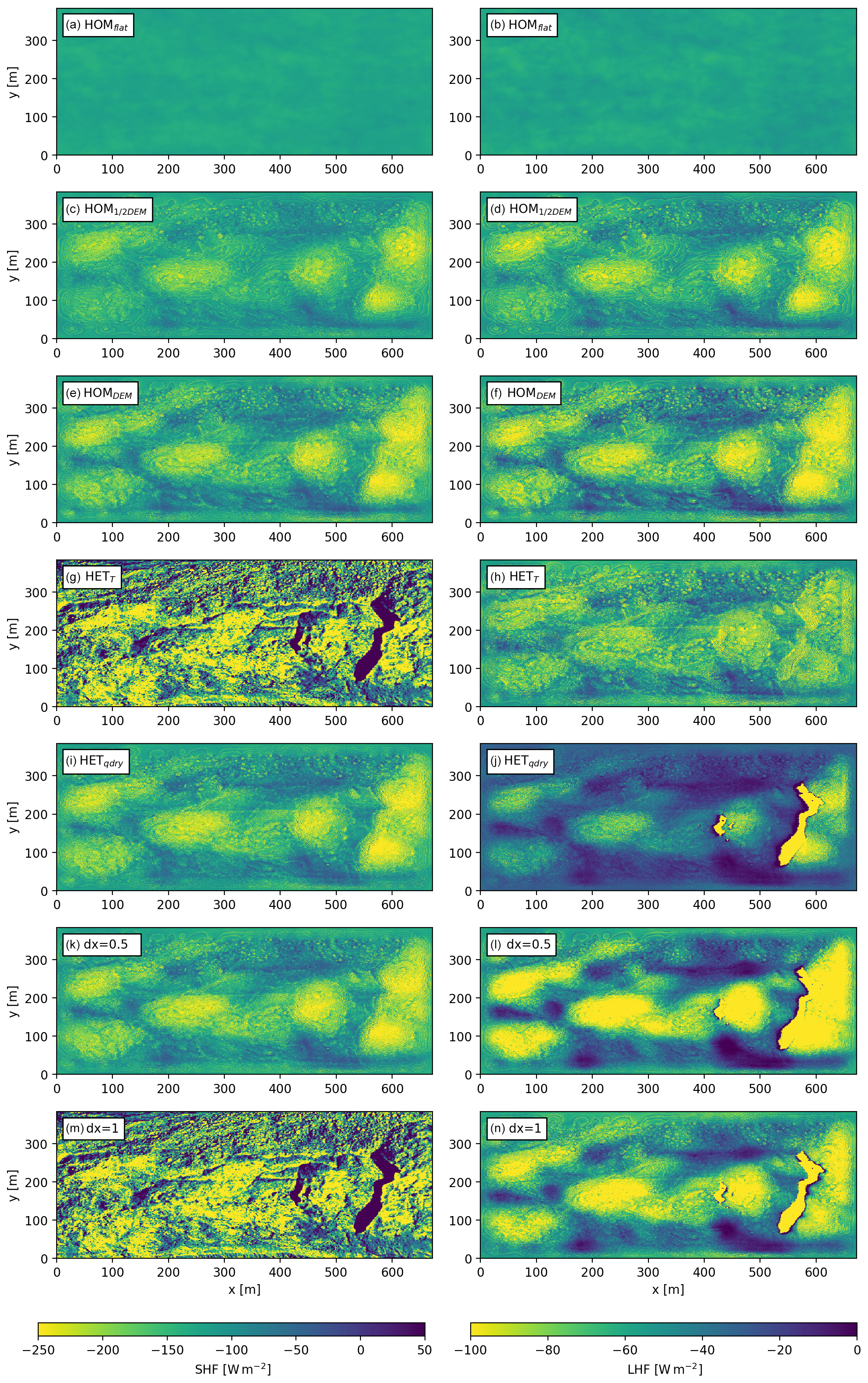
Figure 3Two-dimensional plots of average variables SHF (left panels) and LHF (right panels) for each experiment in the same order as presented in Table 1 (rows). Elevation increases from left to right and the main wind direction is from left to right.

Download

3.1.1 Surface roughness

The effect of surface roughness on the SHF and LHF is evident (Fig. 3a–f). The turbulent fluxes are intensified with increasing variability in topography, since increasing the surface roughness is directly related to the surface roughness length and the generation of turbulence. A homogeneous topography therefore results only in small spatial differences in turbulent fluxes (HOM_flat, 5 and 2 W m⁻² for SHF and LHF respectively). Including a real topography (HOM_DEM) results in more variation of the turbulent fluxes (64 and 30 W m⁻² for SHF and LHF respectively) with the lowest fluxes at higher locations and the highest fluxes in the depressions. This is caused by the combination of an accumulation of heat and moisture in the topographic depressions, and homogeneous surface temperature and specific humidity, resulting in high temperature and moisture gradients.

3.1.2 Surface temperature

The spatially variable temperature (HET_T) has the largest impact on the SHF (Fig. 3g). Prescribing the surface temperature heterogeneously (HET_T) impacts the surface vertical temperature gradient and is therefore extremely important for the SHF. The LHF is less variable in space when including only spatial heterogeneous surface temperatures. This is because the surface temperature pattern is partly inversely related to the topography and the LHF is driven primarily by the moisture gradient. Cold surfaces are now located at the lowest parts of the domain, where it was warmer in HOM_DEM, and LHF is positively related to temperature. Additionally, the spatial variability of the SHF increases from 64 to 193 W m⁻², while the spatial variability in the LHF does not change much (30 vs. 23 W m⁻²). In addition to this, due to the heterogeneous temperatures, positive sensible heat fluxes are present at the locations where the surface is colder than the atmosphere. This is particularly important in understanding the energy balance of ice cliffs and ponds (Sect. 3.5).

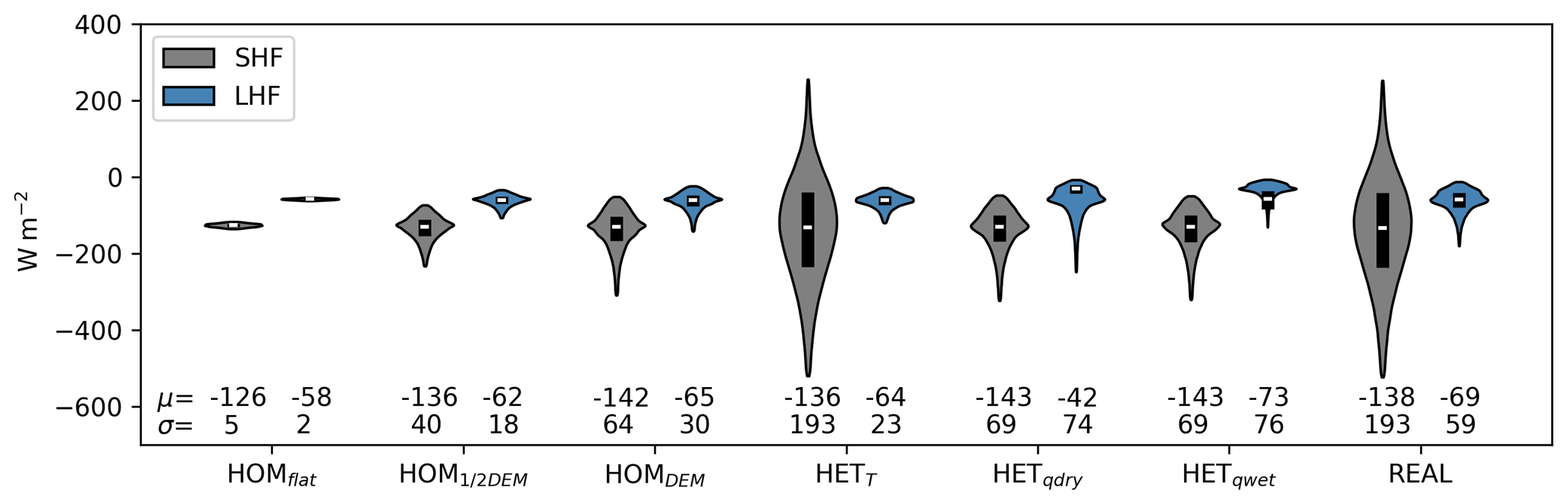
https://www.the-cryosphere.net/14/1611/2020/tc-14-1611-2020-f04

Figure 4Violin plots to show spatial variability of time average fluxes (95 % confidence interval) within the domain for the SHF (grey) and LHF (blue). The numbers indicate the domain average (μ) and standard deviation (σ). Fluxes pointing towards the surface are positive.

Download

3.1.3 Surface specific humidity

The surface specific humidity has the greatest effect on the LHF. The assumption of dry debris (HET $_{q_{dry}}$ ) results in an average LHF of −42 W m⁻². The LHF for moist debris is −73 W m⁻², indicating the important impact of surface moisture on the LHF. A higher surface specific humidity results in more evaporation under the same conditions, given the increase in the vertical moisture gradient at the surface. Moistening the surface (HET $_{q_{wet}}$ ) results in less extreme differences spatially in the LHF, since both experiments include saturated areas at the locations where the real surface temperature is 0 ^∘C. Moistening the surface will increase the atmospheric specific humidity, and, since the relative humidity is fixed for the cliffs at 100 % in both experiments, the variability in specific humidity decreases. Interesting is the high LHF on the leeward side of the ice cliff where the wind transports the moisture originating from the ice cliff over the domain. Note that the main wind flow is from left to right – see Fig. 3.

3.1.4 Spatial variation of elevation, surface temperature and specific humidity

Including spatial variation in specific humidity and surface temperature (real) does not affect the average turbulent fluxes much when compared to homogeneous conditions (HOM_DEM). However the spatial variability is nearly doubled for the sensible heat flux and tripled for the latent heat flux (Fig. 4).

If we assume real as the truth, the sensible and latent heat fluxes will be underestimated by 9 % and 8 % respectively when ignoring the topography (HOM_flat). Assuming both homogeneous surface temperature and specific humidity (HOM_DEM) results in an overestimation of the SHF of 3 % and an underestimation of 4 % of the LHF (Fig. 4).

Increasing the surface roughness has a larger effect on domain-averaged turbulent fluxes than the inclusion of spatial variations for surface temperature or specific humidity. However, prescribing the surface temperature and specific humidity has the greatest impacts on the spatial distribution of the SHF and LHF and results in a high spatial variability. So, for glacier-tongue-wide averages, area averaging of the input variables is justifiable, but if one is interested in detailed spatial patterns of melt it becomes questionable.

3.2 Vertical distribution of temperature, wind and specific humidity

In Figs. 5, 6 and 7 cross sections and vertical profiles of all experiments are shown for the wind speed, specific humidity and potential temperature respectively for the lowest 100 m of the domain. Increasing the surface roughness (HOM_1∕2DEM and HOM_DEM) leads to more mixing of heat and moisture in the atmosphere, due to the higher associated surface roughness length. The topography has a direct influence on the wind speed close to the surface; in depressions the wind speed is low and at high elevations the wind speed increases. Due to the differences in wind speed, the mixing of heat and moisture is also spatially heterogeneous close to the surface. Moisture and heat accumulates in depressions, but wind mixes these regularly into the lower atmosphere.

The vertical profiles are an average of all model grid points above the surface. The mixing of variables extends higher into the atmosphere when the real topography is included. In the real experiment, mixing occurs to an altitude of 40–60 m above the surface, while this is only 20–30 m in HOM_flat. On a larger scale it is established that debris influences the near-surface atmosphere (Collier et al., 2015). We show that the microscale meteorology is also strongly affected by debris, influencing, for example, the local temperature and moisture lapse rates. Heterogeneous surface temperatures allow negative surface temperatures at ice cliffs, resulting in reversed temperature gradients close to the surface (HET_T and real; Fig. 7).

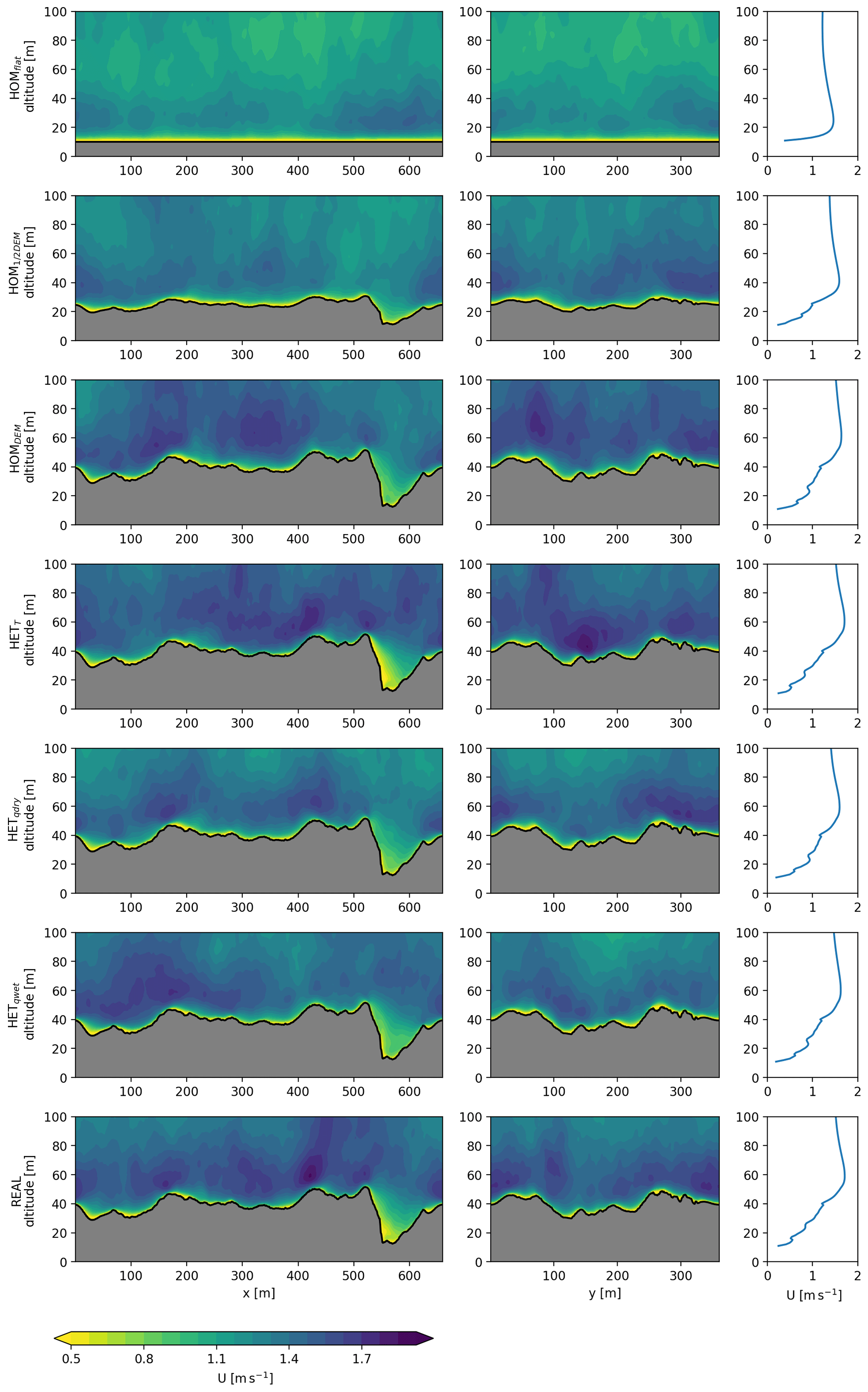
https://www.the-cryosphere.net/14/1611/2020/tc-14-1611-2020-f05

Figure 5Cross sections (left and middle columns) and average vertical profile (right columns) of the wind speed for all experiments presented in the same order as in Table 1. The location of the cross sections is shown in Fig. 2.

Download

The surface roughness causes local differences in wind speeds, especially where there are large elevation differences over a small horizontal range. This is, for example, visible above the ice cliff (x=510–600 m), where the wind gradient decreases towards the bottom. This is confirmed with station observations, where stations at higher locations measure consistently higher wind speeds than at lower locations. The three-dimensional simulation approach used quantifies the spatial differences in wind speed. In local depressions accumulation of heat and moisture frequently occurs, and this is further amplified when including heterogeneous surface specific humidity and temperature. If the accumulated heat and moisture are regularly removed by cold and dry air, these heterogeneous differences create local hot spots of SHF and LHF. Surface roughness can therefore be seen to play an important role and can alter the conductive flux into the debris. At locations where the air is stagnant, fluxes are attenuated since gradients in moisture and temperature between the surface and atmosphere gradually decrease with the accumulation of heat and moisture. Of particular interest are the locations where the specific surface humidity is high and temperature low, such as ice cliffs. We take a more detailed look at these supraglacial features in Sect. 3.5.

https://www.the-cryosphere.net/14/1611/2020/tc-14-1611-2020-f06

Figure 6As in Fig. 5 but here for the specific humidity.

Download

https://www.the-cryosphere.net/14/1611/2020/tc-14-1611-2020-f07

Figure 7As in Fig. 5 but for the potential temperature.

Download

https://www.the-cryosphere.net/14/1611/2020/tc-14-1611-2020-f08

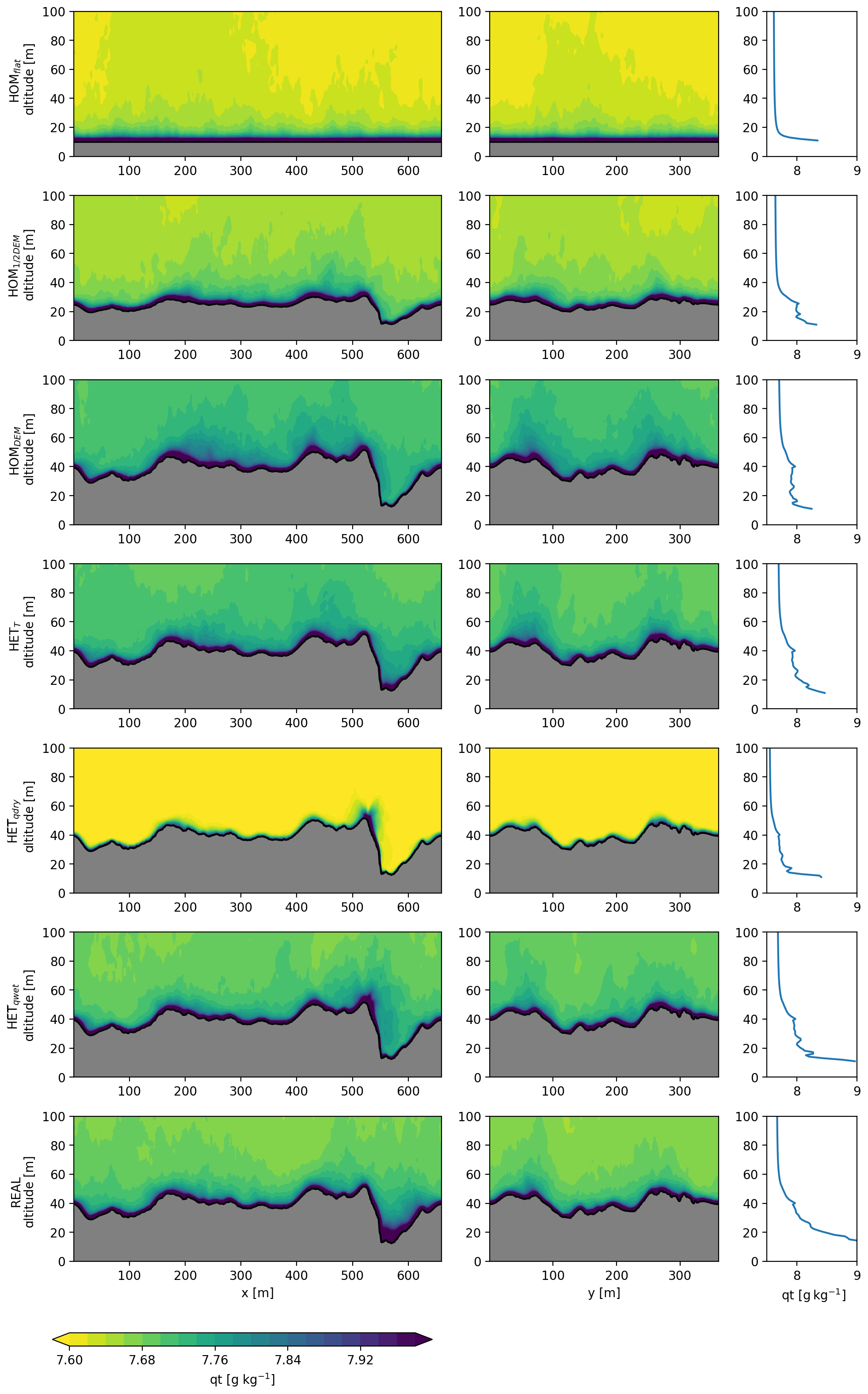
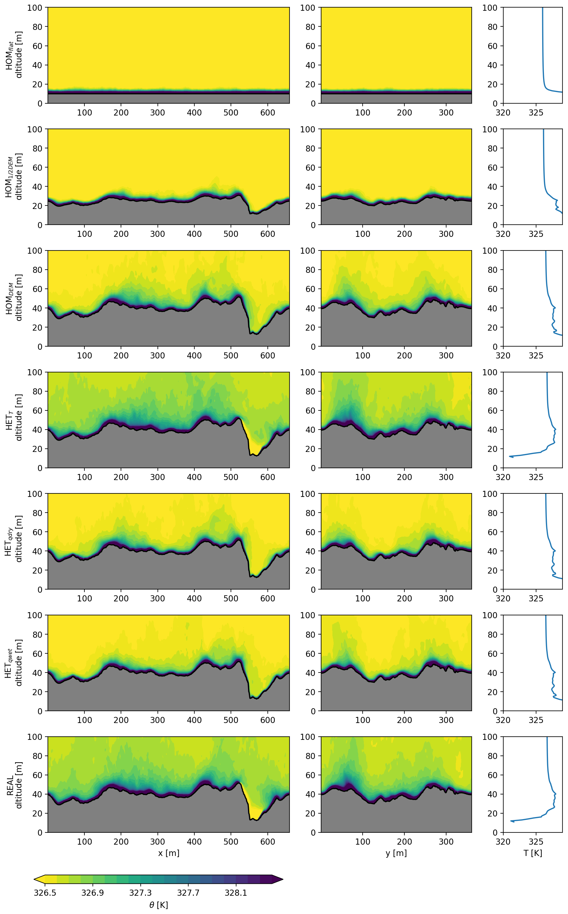
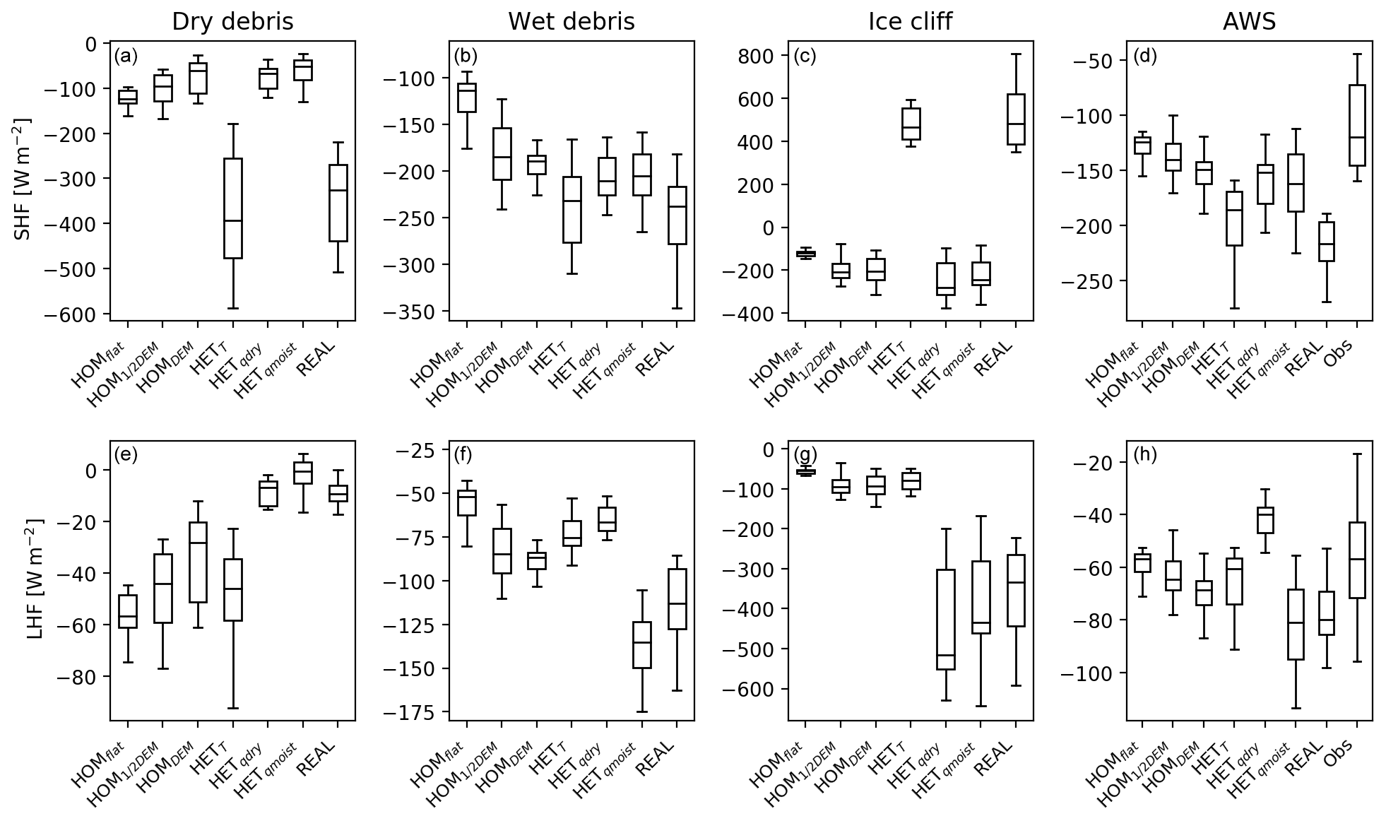
Figure 8Box plots to show variability in possible outcomes at four different locations: dry debris (a, e), wet debris (b, f), ice cliff (c, g; all three points are taken as the average of nine grid points) and AWS location (weighted average over the footprint; d, h) for all experiments (Table 1). Observations (Obs) of the SHF and LHF are shown in (d) and (h). For all simulations the last hour of simulation data is taken and is resampled to a 5 min average. Measurements are averaged over 5 min. The time period taken from the AWS is 10:30–11:30 LT.

Download

3.3 Spatial analysis

In Fig. 8 the possible ranges of the SHF and LHF are plotted for four locations: dry debris (panel a), wet debris (panel b), an ice cliff (panel c) and the location of the AWS (panel d). The exact locations are indicated in Fig. 2. The simulations represent a static state at 11:00 LT, and we interpret the results as a possible range of outcomes for that state. Turbulent fluxes can vary greatly at one location, since they depend on the instantaneous turbulent conditions. This means the variability of turbulent fluxes is large, even with constant surface boundary conditions.

3.3.1 Debris

For comparison between dry and moist debris, two locations are chosen where both surface temperatures are 291 K in the real experiment. Surface moisture values for the dry and wet debris for HET_dry are 8.0 and 8.1 g kg⁻¹, and for HET $_{q_{moist}}$ they are 8.5 and 9.0 g kg⁻¹ respectively. Attributing the differences in fluxes between wet and dry debris to surface moisture is not straightforward since the spatial distribution of surface moisture is dependent on the DEM (dry debris is located at higher-elevated parts, while moist debris is located at depressions). In addition, the surrounding grid points influence the turbulent fluxes. Dry debris is generally located in areas exposed to higher wind speeds and surface roughness, while the opposite holds for wet debris. The SHF is more sensitive to surface temperature for dry debris than for wet debris, and in the real experiment the LHF is approximately 10 times as high over wet debris compared to dry debris. Turbulent fluxes have different sensitivities to surface temperature and moisture, indicating that the sensitivities are different in wet and dry climates. As a result surface boundary conditions should be chosen carefully for simulations.

The LHF over dry debris, when domain averaged (with its spatial standard deviation) in the real case, is lower (q_s<8.4 g kg⁻¹, 34±17 W m⁻²) than over wet debris (q_s>8.8 g kg⁻¹, 117 + 52 W m⁻²). This is caused by less moisture availability. The SHF over wet debris ( $- 237 \pm 247$ W m⁻², excluding ice cliffs) is considerably higher than over dry debris ( $- 135.3 \pm 161$ W m⁻²) and is caused by the location of the wet debris in the depressions, where there is an accumulation of heat that increases the vertical temperature gradient as discussed in Sect. 3.2.

3.3.2 Ice cliff

The surface conditions at an ice cliff are different to those of the surrounding debris surface. This is because the surface is at (or around) melting point and the near-surface air is saturated. As a result the reversed (positive) SHF is the most pronounced difference compared to the debris surface. Additionally, spatially different surface temperatures result in cold and warm eddies that can pass over the ice cliff and increase the variation in the SHF. The variation in the LHF is mainly influenced by the surface specific humidity, since with heterogeneous surface variables dry and wet eddies can flow over the saturated surface, causing different vertical moisture gradients above the ice cliff. This is described in more detail in Sect. 3.5.

3.3.3 AWS measurement comparison

The use of the location of the AWS allows comparison of the simulations to actual measurements. However, while the measurements are an average of the footprint of the station this varies with time and exceeds the domain slightly. We have taken a weighted average over the grid points that are located in the domain. The averaged measured SHF is 49 % lower than the modelled SHF; the LHF is 23 % lower. The range between the first and third quartile for the LHF (SHF) is 16 (36) for the real case and 29 (73) W m⁻² for the observations, showing that the model underestimates the variation. The ranges of simulated LHF overlap with the observed range; however, for the SHF the observed and simulated ranges do not overlap. The comparison between the simulations and the observations gives an indication of the model performance; however, a one-to-one comparison is complex, since our simulations are an idealized representation of the reality in a limited domain and exclude effects of, for example, the moraines or the glacier at higher altitude. The disagreement between simulated and observed fluxes may also be caused by the location of the AWS, which is situated close to the moraines. Steiner et al. (2018) estimated the average surface energy balance for Lirung Glacier at the AWS location to be ±350 W m⁻² for clear sky around 11:00 LT, while in real this is 294.2 W m⁻², using a weighted average for the footprint of the AWS. However the model domain-averaged conductive flux is 348.8 W m⁻², indicating that the model performs well and within a reasonable range.

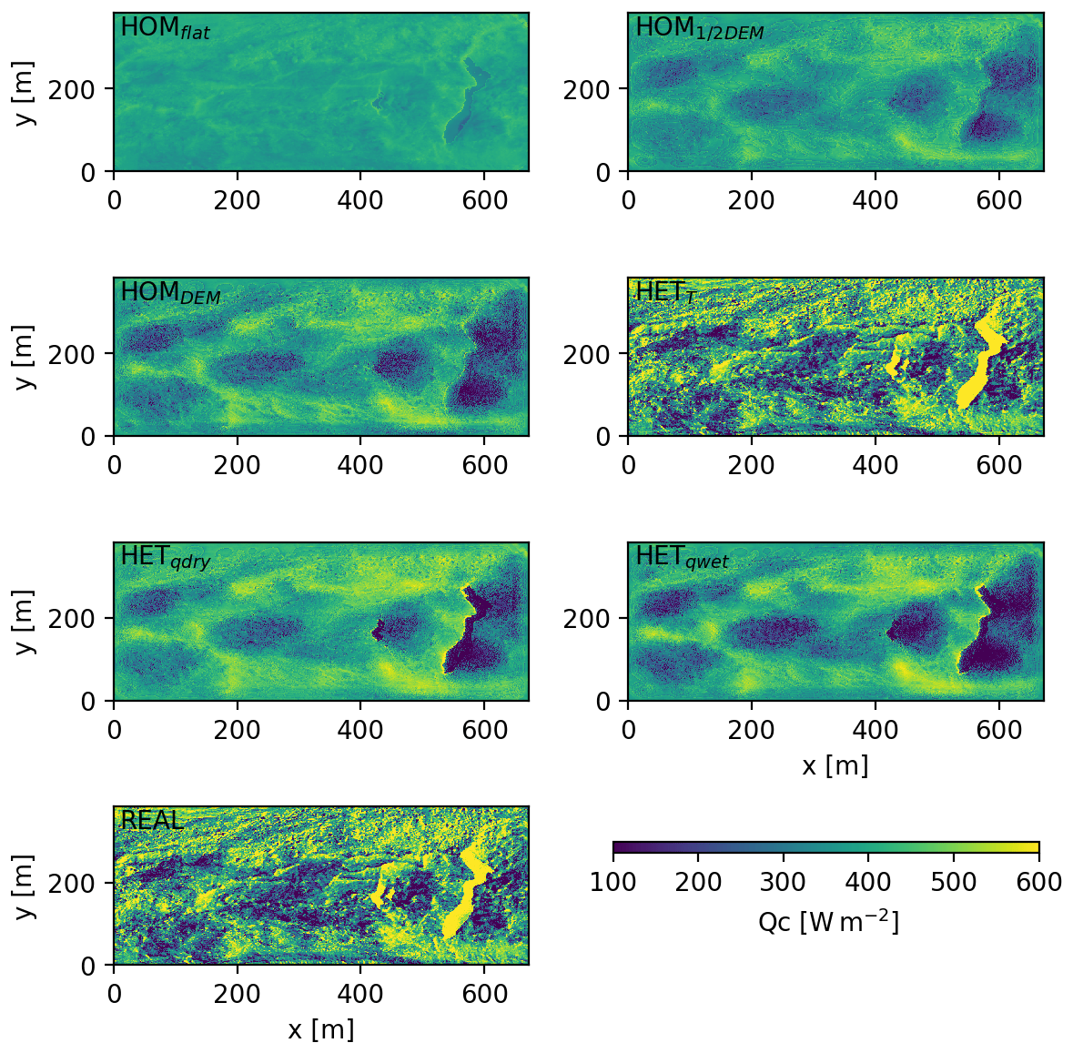
https://www.the-cryosphere.net/14/1611/2020/tc-14-1611-2020-f09

Figure 9Effect of turbulent fluxes on conductive flux into the surface for all experiments. A positive flux means energy is available to go into the surface.

Download

3.4 Surface energy balance

Figure 9 shows conductive flux into the debris under the seven simulations. Spatial heterogeneous shortwave and longwave radiation fields based on the real DEM are used as inputs. The LHF and SHF vary, depending on the experiments to isolate the effects of the individual experiments. For example, the ice cliff signal in Fig. 9a is visible, despite the homogeneous surface conditions in HOM_flat due to the longwave and shortwave signal derived from the real DEM. The energy reaching the ice below the debris is dependent on the thermal conductivity, density and heat capacity of the debris.

With increasing surface roughness (HOM_flat, HOM_1∕2DEM, HOM_DEM) the conductive heat flux becomes more variable, as is also observed for the SHF and LHF separately in Fig. 3. Locally it is important to prescribe the surface specific humidity, e.g. for ice cliffs. A wetter environment results in a lower conductive flux (HET $_{q_{dry}}$ and HET $_{q_{moist}})$ , while a colder surface results in a higher conductive flux (HET_T; Table 2). The effect of the surface temperature (HET_T) is larger than the surface specific humidity (HET $_{q_{moist}}$ ), and therefore the conductive flux of real is closely related to the signal imposed by the surface temperature.

Table 2The average conductive flux averaged over the domain, ice cliff cells and debris cells – with standard deviations. Ice cliffs cover 2 % of the domain. The standard deviation is based on all pixel values in the domain.

Download Print Version | Download XLSX

The aim of this study is to get insight in the spatial variable conductive heat flux, and it goes beyond the scope of present study to investigate the melt dynamics of sub-debris ice. However, this would be an interesting field of future research, and in order to do this spatial variable observations of the thermal conductivity, density and heat capacity of the debris layer are needed, which are currently unavailable. Our interpretation of the results is focused on the surface energy balance and stops at the debris–atmosphere interface.

A heterogeneous conductive flux contributes to heterogeneous melting, depending on the debris thickness. For example in real the average conductive flux on the ice cliffs is 674±76 W m⁻², while this is only 364±191 W m⁻² averaged over the debris. The conductive heat flux at ice cliffs can be used exclusively for ice melt, while for debris the conductive flux is partly used to penetrate and warm the debris. Turbulent fluxes decrease the energy available for melt by 39 % for the real case averaged over the domain. Over debris, turbulent fluxes reduce the available melt energy by 40 % and act as a sink of energy, while on ice cliffs turbulent fluxes enhance it by 51 % and are a contributor to melt. Other studies found that ice cliffs melt between 5.7 and 13.7 times faster than ice below surrounding debris (Brun et al., 2016; Sakai et al., 2002; Reid and Brock, 2014). Although those studies consider total melt rather than the surface energy balance, the pronounced differences between melt on ice cliffs and debris are in line with our research.

The surface specific humidity is relatively uncertain, and the range used in the experiments is based on scarce observations. It is spatially distributed using a simple relation with elevation. We performed additional sensitivity tests of two extreme cases of a homogeneous surface relative humidity of 20 % and of 85 %, with the relative humidity at ice cliffs at 100 %, to quantify the effect on the conductive heat flux. The domain-averaged (± spatial deviation) conductive heat flux when RH = 20 % is 490±201, and it is 89±276 W m⁻² when RH = 85 %. This indicates that the mean conductive flux is positive, regardless of the surface specific humidity. Secondly, if the surface relative humidity is lower than the atmosphere, the latent heat flux is directed towards the surface and contributes to the conductive heat flux. The opposite occurs with a higher relative humidity, which can happen at ponds and ice cliffs. Moreover, the conductive heat flux decreases with increasing relative humidity, which shows the regulating effect of moisture on the total energy budget. At ice cliffs, the latent heat flux can become highly negative if the atmosphere is dry and can even reverse the sign of the conductive heat flux. During the monsoon season (summer months) the surface moisture will be higher than over the rest of the year, and the conductive heat flux at the surface will be higher than in winter and spring.

In summary, these results show turbulent fluxes can be key in explaining the formation of ice cliffs. Locations with already thick debris (and hence higher surface temperatures) do not melt as fast as the surroundings due to the SHF and LHF reducing the conductive flux, as well as the general insulation of the debris (Fig. 9). A crest will develop, introducing the topographic effects as discussed above. This acts as a positive feedback and enhances the local topographic differences on debris-covered glaciers. These results show that turbulent fluxes can be an additional driver for the typically variable topography of a debris-covered tongue and for the formation of ice cliffs, along with collapsing channels, as has been hypothesized (e.g. Benn et al., 2012).

3.5 Ice cliff analysis

Ice cliffs on debris-covered glaciers are particularly interesting to study in terms of turbulence given their steep topography, anomalous surface temperature and moisture conditions compared with the surrounding debris. We showed in the previous section that, on an irregular surface, local hot spots of the conductive flux into the surface exist, amplifying the melt. Such irregularities are likely to favour the formation of ever-deeper depressions and eventually expose ice cliffs. Our simulations do not allow dynamic modelling of ice cliff evolution; however, we can gain insight in the microclimate around such cliffs to better understand the fundamental mechanisms of ice cliff melting. Three-dimensional modelling can thus provide insight into processes such as advection of heat and moisture.

In Fig. 10 six vertical profiles of wind speed, potential temperature and specific humidity over an ice cliff are shown with a time interval of 10 s. On the leeward side of an ice cliff eddies are generated by both the thermal and moisture gradients and the topography. In the situation we examine the clean ice is on the left side of the local depression and the dominant wind flow is from the left to right. When relatively warm air is advected over the ice cliff, this air cools, falls down (first column), and generates an eddy where the accumulated moisture is transported out of the depression and the cold air is replaced by warmer air (columns 2–3). At this point the SHF and LHF are intensified, since the moisture and temperature gradients are increased within the depression. Intensification of the turbulent fluxes occurs, since warm air from the right side of the depression is transported towards the clean ice by the rotating eddy (column 4). After such an advection event the ice will cool and moisten the air in the depression. The vertical moisture and temperature gradients decrease in time, and the SHF and LHF decrease until the process of refreshment repeats itself.

During an advection event warm and dry air flows over the ice cliff and is transported into the depression. This causes (temporarily) a strong gradient, and sensible heat contributes to melt, until the air has cooled down. This process gives an intensified melt signal at the ice cliff and causes it to deepen and, in this specific case, to retreat to the left. This is congruent with ice cliff backwasting found in previous studies (Reid and Brock, 2014; Steiner et al., 2015). Similarly, Mott et al. (2014) found that net surface radiation over snow patches is not the only driver of energy exchange between the surface and atmosphere in mountainous areas, with secondary flows induced by surface heterogeneities also being an important driver. We hypothesize that ice cliff backwasting can also be related to the main wind direction in the domain. Cliffs that are in the leeward direction of the main wind direction during daytime receive additional warm dry air through the advection mechanism, causing extra melt.

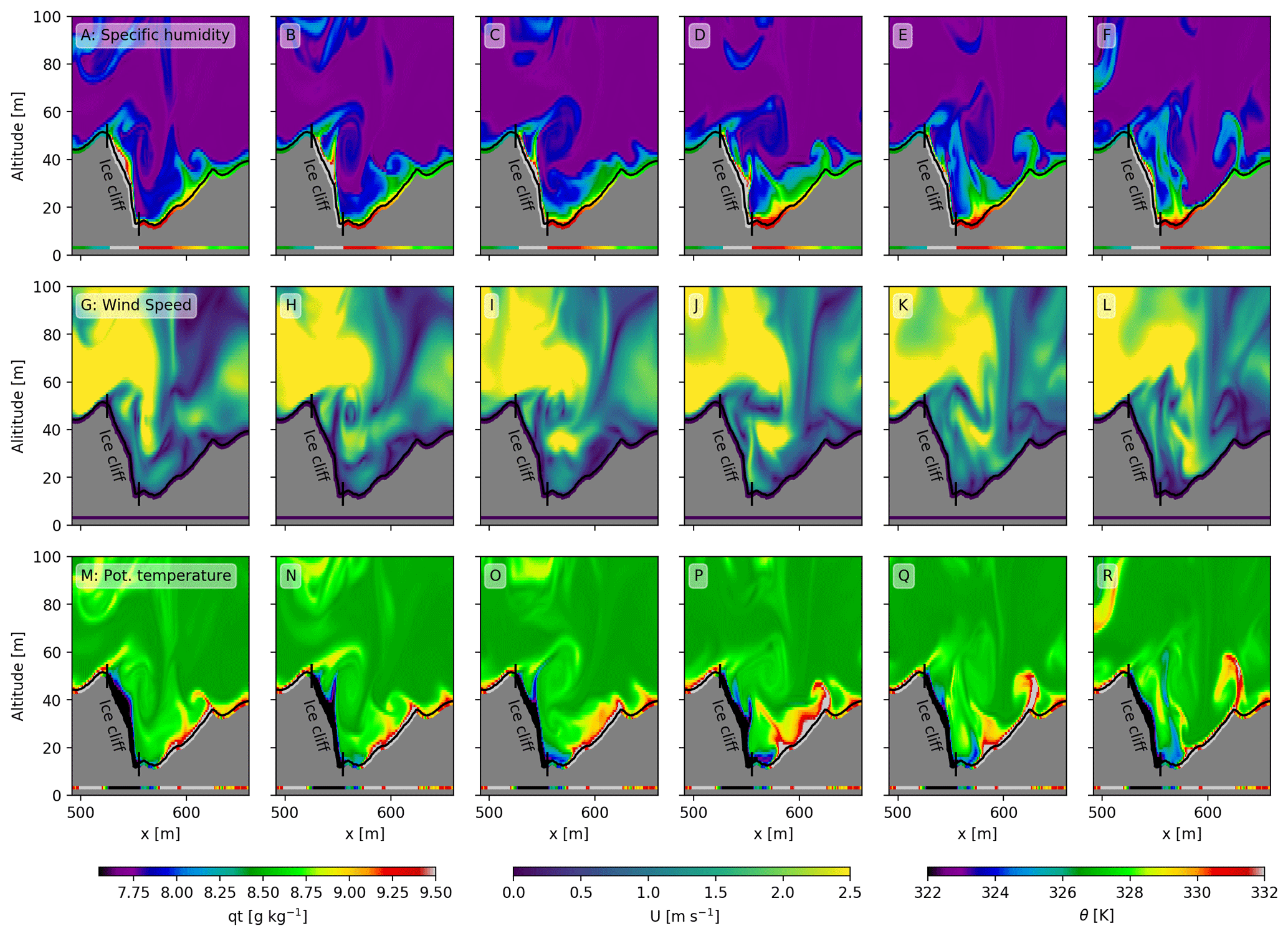
https://www.the-cryosphere.net/14/1611/2020/tc-14-1611-2020-f10

Figure 10The specific humidity (a–f), wind speed (g–l) and temperature (m–r) for a close-up around an ice cliff ( $660 < x > 500$ m) at time = 6570–6630 s with a 10 s time interval. The black line indicates the topography. The surface boundary conditions are plotted directly below the surface and, for clarity, also at y=0.

Download

Ice cliffs typically have a knick-point shape, previously explained by differences in local radiation (Sakai et al., 2002). However this explanation ignores the extra amount of longwave radiation in the depressions (Steiner et al., 2015) and does not explain why crests generally do not flatten over time. Turbulent fluxes are also likely to play a role in the shape of the ice cliffs as a result of the vertical variations in wind speed induced by the topography. This can be seen in Fig. 5, where the wind speed decreases with depth at the ice cliff (x=550 m), and the knick point of the ice cliff is at the location of strongest decline in wind speed. The heat and moisture exchange are therefore strongest at the top of the ice cliff and lowest in the depression, with the main wind flow being over the depression and not reaching the deepest parts of the ice cliff.

4 Sensitivity to Reynolds number

In order to simulate atmospheric turbulent flows there are two options: DNS and LES. Both options come with advantages and drawbacks. DNS is computationally extremely expensive when resolving all scales in the flow, and its use was not possible in our case study. An advantage of DNS is that the correctness of a simulation can be checked by testing whether the results of sensitivity tests converge, as we will do in this section. With LES however this approach would not be possible, as sensitivity tests can even be wrongly caused by the inappropriate surface model under high Reynolds numbers in complex terrain. This means that even when resolving all scales in the flow with LES, this does not give direct confidence in the results and LES does not outperform DNS by definition.

The Reynolds number (Re) is a measure for the flow characteristics and is the ratio between inertial and viscous forces in a fluid (Eq. 18). A low Reynolds number would indicate a laminar flow and a high Reynolds number a turbulent flow.

\begin{matrix} (18) & Re = \frac{u L}{ν}, \end{matrix}

where u is the velocity (m s⁻¹), L is the characteristic length scale (m) and ν is the kinematic viscosity (m² s⁻¹) of the fluid. By decreasing the kinematic viscosity the fluid will become more turbulent and resolve smaller scales.

To show that turbulence is fully developed in our study, we double the Reynolds number by decreasing the viscosity from 0.2 to 0.11 m² s⁻¹, and we repeated the real experiment. Computationally the run with low viscosity is 15 times more demanding than the high viscosity as the viscosity is halved and the number of grid points is doubled in x, y and z. The LHF and SHF have the same patterns and are in same order of magnitude at both viscosities (Fig. A1). Furthermore, the averaged vertical profiles of potential temperature and specific moisture are also similar, which gives confidence in the use of 1 m resolution for this type of simulations (Fig. A2).

The energy spectrum of specific humidity is shown in Fig. A3; energy spectra of other variables (e.g. temperature and wind) show the same pattern. As this run is very complex and far from idealized, comparison of energy spectra of the viscosities is not straightforward. The energy spectra are derived from a horizontal cross section at a fixed height of 65 m above the lowest point in the topography, implying that the cross section is not at a constant height above the surface. As a result, the spectrum contains not only a signature of the turbulence but also of the topography. The peak of the spectrum is located around a wave number of 1, which corresponds to a wavelength of $2 π / 1 \approx 6$ m and is resolved by both experiments. This shows that large structures are dominant in the flow and small structures are of minor importance. The spectra averages for both experiments differ, although they located in the centre of the bandwidth of 1 standard deviation.

The simulation at low viscosity naturally resolves smaller scales than the simulation with a higher viscosity (see Eq. 18). In Fig. A3 we see that the additional variability only adds a small amount of variance to the signal and is therefore irrelevant for the flow (wave numbers > 11). We therefore conclude that a viscosity of 0.2 m² s⁻¹, in combination with a spatial resolution of 1 m, is fine enough to capture the bulk characteristics of the flow as well as its most important features.

5 Limitations

There is an initial but incomplete understanding of micrometeorological processes for debris-covered glaciers with highly variable surface temperature and moisture conditions. In particular the role that turbulent fluxes have in the net conductive energy flux towards the ice below the debris is unknown. For the first time, in this study, a 3D turbulence-resolving high-resolution model was used to gain understanding of these local processes and interactions between the surface and the overlying atmosphere. We show that such turbulence-resolving models provide important insights into these processes, supporting a better quantification of debris-covered glacier melt. However, we identified a number of limitations associated with data availability, the model assumptions and computational constraints, which we discuss in the following paragraphs.

Information about surface moisture on debris-covered glaciers is scarce and highly variable, and measurement is difficult. Surface moisture is, however, an important variable in assessing the surface energy balance since it influences the latent and sensible heat flux and therefore the conductive heat flux that ultimately melts the ice. Studies normally deal with the limited information available for surface moisture by assuming that the debris surface is either dry or fully saturated to indicate the range of outcomes (e.g. Rounce et al., 2015). The approach proposed in this study is a step towards a better representation of surface specific humidity, showing the effect of a partly saturated surface and, furthermore, a heterogeneous distribution linked to the DEM. In reality the surface moisture is dependent on the surface material and texture, its relative elevation in the domain, and the aspect of the location (Qiu et al., 2001). In future, the spatial distribution could also be made dependent on debris grain size rather than the absolute height of the topography in order to make spatial patterns of surface specific humidity more realistic. During our observation period no large supraglacial ponds were observed (Fig. 1), but surface conditions of ponds could also be included in MicroHH in upcoming studies.

In this study we have considered the conductive heat flux and how this brings about a gradual warming of the debris, eventually melting the ice when the warming front reaches the debris–ice interface. How this energy is partitioned between the warming of the debris and melting depends on the debris thickness, the type of rock, the texture and the moisture content. Future studies can couple a debris energy balance model (e.g. Giese, 2019; Reid and Brock, 2010) to MicroHH, investigating the total energy reaching the ice, its timing, and the impact of debris properties such as thickness, surface moisture and thermal conductivity.

One of our experimental outcomes is that the use of spatially variable surface boundary conditions for surface specific humidity and temperature results in similar domain averages of turbulent surface fluxes compared to a constant surface temperature or specific humidity. This all relies on the strong assumption that the homogeneous value (in reality taken from a weather station measurement) is representative of the whole domain. In our experiments the homogeneous value is per definition representative for the domain, as it is an average of the heterogeneous values. The bias induced by upscaling point measurements is given by comparing the results of the homogeneous surface conditions (HOM experiments) and the heterogeneous surface conditions (HET experiments). This shows that heterogeneity plays an important role for local supraglacial features on a debris-covered glacier, while the domain-averaged effects on the conductive heat flux are minor. In reality it is close to impossible to locate a station so that it is perfectly representative of the whole domain without having prior knowledge of the spatial distribution. This type of high-resolution modelling can therefore support the optimal selection of sites for meteorological observations to ensure representativity.

High-resolution modelling is a useful tool to investigate small-scale meteorological processes, due to its explicit treatment of turbulent processes. The modelling is, at this stage, still conceptual, since not all processes and feedbacks are included. In this study only a part of Lirung Glacier is modelled, and the modelling excludes surrounding influences such as wind flows caused by the lateral moraines and circulations in the valley. Due to the high spatial resolution and computational constraints, we limited the simulation time to 1 h and the simulation is stationary.

A correct representation of debris-covered glaciers would benefit climate, glacier and hydrological models to give a better estimation of meltwater contribution to river discharge. Our study provided important insights but also made clear that turbulence-resolving, long-term and transient simulations are currently not feasible. Our results nevertheless do provide a greater understanding of surface processes on debris-covered glaciers along with parameterizations that can be used in coarser-resolution models. In order to understand the small-scale processes at the surface–atmosphere interface on a debris-covered glacier, we need high-resolution data and models.

6 Conclusions

The exact melt processes of debris-covered glaciers are largely unknown, and their total contribution to the total glacier melt remains uncertain. The surface of a debris-covered glacier is complex due to its topography, heterogeneous surface temperature and surface moisture – resulting in highly heterogeneous micrometeorological conditions. In this study, we assess the effect of surface properties of debris on the spatial distribution of micro meteorological variables, such as wind fields, moisture and temperature by sensitivity tests. Subsequently we investigated how those drive the turbulent fluxes and eventually the conductive heat flux for a debris-covered glacier. This is the first time an in-depth analysis has been performed of micrometeorological variables above a debris-covered glacier with a turbulence-resolving model at high resolution (∼ 1 m). This has offered new insights into the spatial variability of turbulent fluxes and what drives these differences.

Surface roughness has the strongest impact on the magnitude of turbulent fluxes and leads to more mixing at higher altitudes due to the higher topographic variability. Surface roughness causes spatial differences in wind speed, with generally lower wind speeds at lower elevations due to isolation, whereby accumulation of heat and moisture is possible. Increasing the surface roughness therefore leads to more pronounced spatial differences in turbulent fluxes.

Heterogeneous surface temperature has its primary impact on the SHF; this is because of the way it influences the temperature gradient between the surface and the atmosphere. A heterogeneous surface specific humidity affects mainly the LHF by influencing the moisture gradient between the surface and the atmosphere. Overall, including heterogeneous conditions leads to higher spatial variability and a larger range of possible outcomes. The variability of the turbulent fluxes can result in a feedback effect that eventually leads to the hummocky terrain typical for debris-covered tongues in the Himalaya. In more extreme cases this variability can bring about the formation of cliffs and also of ponds in those depressions where melt has been accelerated.

We found that the inclusion of heterogeneous surface temperature and specific humidity is extremely important when looking at sub-glacier features such as ice cliffs as these allow both negative and positive turbulent fluxes in the domain. The microclimate around an ice cliff is influenced strongly by a combination of topographic, surface specific moisture and temperature effects, which favour high sensible and latent heat fluxes. Additionally the progression and persistence of ice cliffs is influenced by the main wind direction, since at the leeward side of the cliff turbulent fluxes contribute to melt. Longer high-resolution turbulence-resolving simulations are needed to investigate fundamentals of small-scale glacier features in more detail.

We show that turbulent fluxes can decrease the energy available for melt at the debris surface by 40 %, acting as an energy sink. In contrast, on ice cliffs turbulent fluxes were found to enhance the available energy by 51 %, serving as a contributor to melt. In combination with a low albedo this causes ice cliffs to be melt hot spots.

The use of homogeneous surface temperature and specific humidity is a good alternative when spatial data are lacking but only when these values are representative of the whole domain and the interest is primarily in domain-averaged outcomes. In general a point measurement will not be representative for the whole domain, and use will result in large biases in atmospheric variables when upscaling to a larger area.

Our results show that high-resolution turbulence-resolving models can be used to better quantify spatially variable melt. Future studies could couple high-resolution models to a full energy balance model to determine the energy reaching the ice. This work is important for glacier mass balance modelling and for the understanding of the evolution of debris-covered glaciers. We expect that these results will be useful in improving the representation of debris-covered glaciers in hydrological and climatological models to determine their contribution to glacier melt.

Appendix A

This appendix presents the most relevant results of a sensitivity study to the Reynolds number. With this analysis we demonstrate that the results in the main text do not change when halving the Reynolds number. To provide an intuitive insight into this, Fig. A1 shows the computed surface sensible and latent heat fluxes for both simulations. This figure clearly demonstrates nearly identical patterns and magnitudes of the surface fluxes. The similarity can also be understood from scaling arguments. Over a rough surface, the wind-driven surface fluxes can be approximated as

\begin{aligned} LHF = ρ \cdot L_{v} \cdot c_{d_{q}} \cdot (u - u_{0}) \cdot (q - q_{0}), \\ SHF = ρ \cdot c_{p} \cdot c_{d_{h}} \cdot (u - u_{0}) \cdot (T - T_{0}), \end{aligned}

where ρ is the air density, c_p the specific heat, $C_{d_{h}}$ and $C_{d_{q}}$ the exchange coefficients for heat and moisture respectively, u the wind speed, u₀ the wind speed at the surface, T the temperature and T₀ the temperature at the surface, L_v the latent heat of vaporization, q the specific humidity, and q₀ the specific humidity at the surface. In our case both simulations have the same boundary conditions for temperature and humidity and resolve nearly identical atmospheric fields (Fig. A2). As atmospheric profiles are identical, the only place where low Reynolds number effects could manifest is via $C_{d_{h}}$ and $C_{d_{q}}$ and therefore in the magnitude of the surface fluxes, yet Fig. A1 shows that this is not the case.

Further proof of the independence of the bulk quantities (profiles of means and variances) can be found in the streamwise spectra of specific humidity (Fig. A3). The additional variance that is resolved in wave numbers > 11 does not contribute significantly to the total variance. This can be visually inferred from Fig. A3, as the total variance is the area under the graph, and the newly added variance is invisible to the eye.

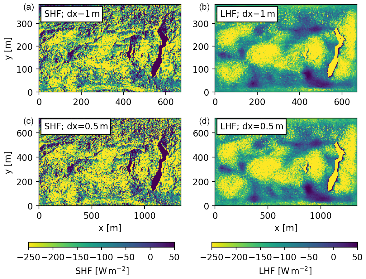
https://www.the-cryosphere.net/14/1611/2020/tc-14-1611-2020-f11

Figure A1The averaged sensible (a, c) and latent heat flux (b, d) for the real experiment with a viscosity of 0.2 m² s⁻¹ (dx = 1 m; a ,b) and with viscosity of 0.11 m² s⁻¹ (dx = 0.5 m; c, d).

Download

https://www.the-cryosphere.net/14/1611/2020/tc-14-1611-2020-f12

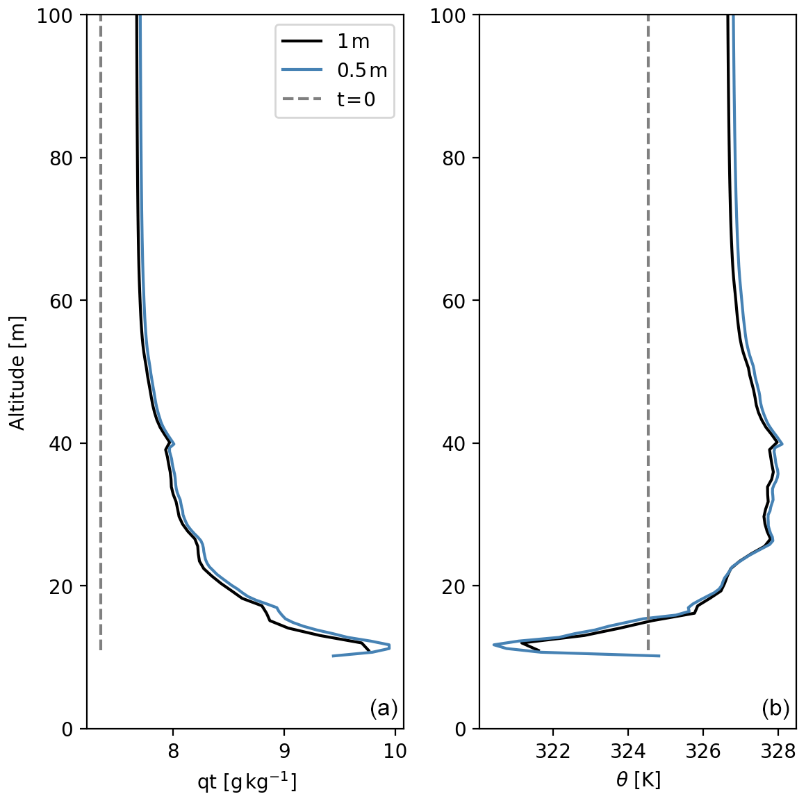
Figure A2Total specific humidity (a) potential temperature (b) profiles for the real experiment with dx= 1 m (black), dx= 0.5 m (blue) averaged over the simulation hour and their initial profiles at t=0 (grey).

Download

https://www.the-cryosphere.net/14/1611/2020/tc-14-1611-2020-f13

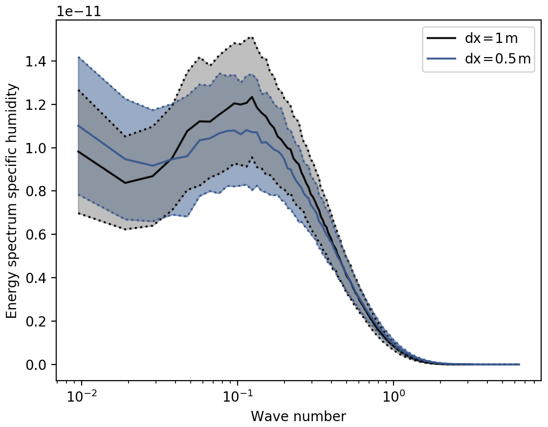
Figure A3Energy spectrum for the total specific humidity at 65 m above lowest point of the topography, averaged over the simulation hour. Shading indicates 1 standard deviation. The vertical axis is premultiplied with the wave number.

Download

Data availability

The data can be found at https://doi.org/10.5281/zenodo.3375325 (Bonekamp et al., 2019b) and https://doi.org/10.5281/zenodo.3375490 (Bonekamp et al., 2019c).

Video supplement

Supporting movies are available at https://doi.org/10.5281/zenodo.3375333 (Bonekamp et al., 2019d).

Author contributions

PB designed the study together with WI. CH adjusted the MicroHH model for this study. PB performed all numerical experiments and prepared the manuscript with contributions from all co-authors.

Competing interests

The authors declare that they have no conflict of interest.

Acknowledgements

This project has received funding from the European Research Council (ERC) under the European Union Horizon 2020 research and innovation programme (grant agreement no. 676819) and the Netherlands Organization for Scientific Research under the Innovational Research Incentives Scheme VIDI (grant agreement no. 016.181.308). Supercomputing resources were financially supported by the Dutch Research Council (NWO) and provided by SURFsara (https://www.surf.nl/, last access: 15 October 2019) on the Cartesius cluster. We thank Joseph Shea and Maxime Litt for setting up the measurement station. We are grateful to the trekking agency Glacier Safari Treks and their staff, without whom this work would not have been possible. We thank ICIMOD for their scientific support and facilitation of the fieldwork. The immersed boundary code is developed as part of NWO project 864.14.007. We thank Bart van Stratum for his valuable help with the immersed boundary layer implementation and the challenges over steep orography.

Financial support

This research has been supported by the Nederlandse Organisatie voor Wetenschappelijk Onderzoek (grant no. 016.181.308), the H2020 European Research Council (CAT, grant no. 676819), and the NWO project (864.14.007).

Review statement

This paper was edited by Tobias Sauter and reviewed by two anonymous referees.

References

Ahlers, G., Grossmann, S., and Lohse, D.: Heat transfer and large scale dynamics in turbulent Rayleigh-Bénard convection, Rev. Mod. Phys., 81, 503–538, https://doi.org/10.1103/RevModPhys.81.503, 2009.

Ansorge, C. and Mellado, J. P.: Analyses of external and global intermittency in the logarithmic layer of Ekman flow, J. Fluid Mech., 805, 611–635, https://doi.org/10.1017/jfm.2016.534, 2016.

Axelsen, S. L. and van Dop, H.: Large-eddy simulation of katabatic winds. Part 1: Comparison with observations, Acta Geophys., 57, 803–836, https://doi.org/10.2478/s11600-009-0041-6, 2009a.

Axelsen, S. L. and van Dop, H.: Large-Eddy simulation of katabatic winds. Part 2: Sensitivity study and comparison with analytical models, Acta Geophys., 57, 837–856, https://doi.org/10.2478/s11600-009-0042-5, 2009b.

Benn, D. I., Thompson, S., Gulley, J., Mertes, J., Luckman, A., and Nicholson, L.: Structure and evolution of the drainage system of a Himalayan debris-covered glacier, and its relationship with patterns of mass loss, The Cryosphere, 11, 2247–2264, https://doi.org/10.5194/tc-11-2247-2017, 2017.

Benn, D. I., Bolch, T., Hands, K., Gulley, J., Luckman, A., Nicholson, L. I., Quincey, D., Thompson, S., Toumi, R., and Wiseman, S.: Response of debris-covered glaciers in the Mount Everest region to recent warming, and implications for outburst flood hazards, Earth-Science Rev., 114, 156–174, https://doi.org/10.1016/j.earscirev.2012.03.008, 2012.

Bonekamp, P. N. J., de Kok, R. J., Collier, E., and Immerzeel, W. W.: Contrasting Meteorological Drivers of the Glacier Mass Balance Between the Karakoram and Central Himalaya, Front. Earth Sci., 7, 1–14, https://doi.org/10.3389/feart.2019.00107, 2019a.

Bonekamp, P. N. J., van Heerwaarden, C. C., Steiner, J. F., and Immerzeel, W. W.: Simulation output of Lirung glacier, Zenodo, https://doi.org/10.5281/zenodo.3375325, 2019b.

Bonekamp, P. N. J., van Heerwaarden, C. C., Steiner, J. F., and Immerzeel, W. W.: Simulation output of Lirung glacier (REAL EXP), Zenodo, https://doi.org/10.5281/zenodo.3375490, 2019c.

Bonekamp, P. N. J., van Heerwaarden, C. C., Steiner, J. F., and Immerzeel, W. W.: Supporting videos of (ice cliffs of) Lirung glacier, Zenodo, https://doi.org/10.5281/zenodo.3375333, 2019d.

Brun, F., Buri, P., Miles, E. S., Wagnon, P., Steiner, J., Berthier, E., Ragettli, S., Kraaijenbrink, P., Immerzeel, W. W., and Pellicciotti, F.: Quantifying volume loss from ice cliffs on debris-covered glaciers using high-resolution terrestrial and aerial photogrammetry, J. Glaciol., 62, 684–695, https://doi.org/10.1017/jog.2016.54, 2016.

Buri, P. and Pellicciotti, F.: Aspect controls the survival of ice cliffs on debris-covered glaciers, P. Natl. Acad. Sci. USA, 115, 4369–4374, https://doi.org/10.1073/pnas.1713892115, 2018.

Buri, P., Pellicciotti, F., Steiner, J. F., Miles, E. S., and Immerzeel, W. W.: A grid-based model of backwasting of supraglacial ice cliffs on debris-covered glaciers, Ann. Glaciol., 57, 199–211, https://doi.org/10.3189/2016AoG71A059, 2016a.

Buri, P., Miles, E. S., Steiner, J. F., Immerzeel, W. W., Wagnon, P., and Pellicciotti, F.: A physically based 3-D model of ice cliff evolution over debris-covered glaciers, J. Geophys. Res.-Earth Surf., 121, 2471–2493, https://doi.org/10.1002/2016JF004039, 2016b.

Collier, E. and Immerzeel, W. W.: High-resolution modeling of atmospheric dynamics in the Nepalese Himalaya, J. Geophys. Res.-Atmos., 120, 9882–9896, https://doi.org/10.1002/2015JD023266, 2015.

Collier, E., Mölg, T., Maussion, F., Scherer, D., Mayer, C., and Bush, A. B. G.: High-resolution interactive modelling of the mountain glacier–atmosphere interface: an application over the Karakoram, The Cryosphere, 7, 779–795, https://doi.org/10.5194/tc-7-779-2013, 2013.

Collier, E., Maussion, F., Nicholson, L. I., Mölg, T., Immerzeel, W. W., and Bush, A. B. G.: Impact of debris cover on glacier ablation and atmosphere–glacier feedbacks in the Karakoram, The Cryosphere, 9, 1617–1632, https://doi.org/10.5194/tc-9-1617-2015, 2015.

Dimotakis, P. E.: The mixing transition in turbulent flows, J. Fluid Mech., 409, 69–98, https://doi.org/10.1017/S0022112099007946, 2000.

Fyffe, C. L., Reid, T. D., Brock, B. W., Kirkbride, M. P., Diolaiuti, G., Smiraglia, C., and Diotri, F.: A distributed energy-balance melt model of an alpine debris-covered glacier, J. Glaciol., 60, 587–602, https://doi.org/10.3189/2014JoG13J148, 2014.

Giese, A.: Heat flow, energy balance, and radar propagation: porous media studies applied to the melt of Changri Nup Glacier, Nepal Himalayas, Doctoral dissertation, Darthmonth College, Hanover, New Hampshire, 2019.

Immerzeel, W. W., Kraaijenbrink, P. D. A., Shea, J. M., Shrestha, A. B., Pellicciotti, F., Bierkens, M. F. P., and de Jong, S. M.: High-resolution monitoring of Himalayan glacier dynamics using unmanned aerial vehicles, Remote Sens. Environ., 150, 93–103, https://doi.org/10.1016/j.rse.2014.04.025, 2014a.

Immerzeel, W. W., Petersen, L., Ragettli, S., and Pellicciotti, F.: The importance of observed gradients of air temperature and precipitation for modeling runoff from a glacierized watershed in the Nepalese Himalayas, Water Resour. Res., 50, 2212–2226, https://doi.org/10.1002/2013WR014506, 2014b.

Kraaijenbrink, P. D. A., Shea, J. M. M., Pellicciotti, F., De Jong, S. M., Immerzeel, W. W., Jong, S. M. D., and Immerzeel, W. W. W.: Object-based analysis of unmanned aerial vehicle imagery to map and characterise surface features on a debris-covered glacier, Remote Sens. Environ., 186, 581–595, https://doi.org/10.1016/j.rse.2016.09.013, 2016.

Kraaijenbrink, P. D. A., Bierkens, M. F. P., Lutz, A. F., and Immerzeel, W. W.: Impact of a global temperature rise of 1.5 degrees Celsius on Asia's glaciers, Nature, 549, 257–260, 2017.

Kraaijenbrink, P. D. A., Shea, J. M., Litt, M., Steiner, J. F., Treichler, D., Koch, I., and Immerzeel, W. W.: Mapping surface temperatures on a debris-covered glacier with an unmanned aerial vehicle, Front. Earth Sci., 6, 64, https://doi.org/10.3389/feart.2018.00064, 2018.

Lejeune, Y., Bertrand, J. M., Wagnon, P., and Morin, S.: A physically based model of the year-round surface energy and mass balance of debris-covered glaciers, J. Glaciol., 59, 327–344, https://doi.org/10.3189/2013JoG12J149, 2013.

Lutz, A. F., Immerzeel, W. W., Gobiet, A., Pellicciotti, F., and Bierkens, M. F. P.: Comparison of climate change signals in CMIP3 and CMIP5 multi-model ensembles and implications for Central Asian glaciers, Hydrol. Earth Syst. Sci., 17, 3661–3677, https://doi.org/10.5194/hess-17-3661-2013, 2013.

McCarthy, M., Pritchard, H., Willis, I., and King, E.: Ground-penetrating radar measurements of debris thickness on Lirung Glacier, Nepal, J. Glaciol., 63, 543–555, https://doi.org/10.1017/jog.2017.18, 2017.

Mellado, J. P.: Direct numerical simulation of free convection over a heated plate, J. Fluid Mech., 712, 418–450, https://doi.org/10.1017/jfm.2012.428, 2012.

Mihalcea, C., Mayer, C., Diolaiuti, G., D'Agata, C., Smiraglia, C., Lambrecht, A., Vuillermoz, E., and Tartari, G.: Spatial distribution of debris thickness and melting from remote-sensing and meteorological data, at debris-covered Baltoro glacier, Karakoram, Pakistan, Annals of Glaciology, 48, 49–57, 2008.

Miles, E. S., Pellicciotti, F., Willis, I. C., Steiner, J. F., Buri, P., and Arnold, N. S.: Refined energy-balance modelling of a supraglacial pond, Langtang Khola, Nepal, Ann. Glaciol., 57, 29–40, https://doi.org/10.3189/2016AoG71A421, 2016.

Miles, E. S., Steiner, J. F., and Brun, F.: Highly variable aerodynamic roughness length (z₀) for a hummocky debris-covered glacier, J. Geophys. Res.-Atmos., 122, 8447–8466, https://doi.org/10.1002/2017JD026510, 2017a.

Miles, E. S., Steiner, J., Willis, I., Buri, P., Immerzeel, W. W., Chesnokova, A., and Pellicciotti, F.: Pond Dynamics and Supraglacial-Englacial Connectivity on Debris-Covered Lirung Glacier, Nepal, Front. Earth Sci., 5, 69, https://doi.org/10.3389/feart.2017.00069, 2017b.

Miles, E. S., Willis, I., Buri, P., Steiner, J. F., Arnold, N. S., and Pellicciotti, F.: Surface Pond Energy Absorption Across Four Himalayan Glaciers Accounts for 1/8 of Total Catchment Ice Loss, Geophys. Res. Lett., 45, 10464–10473, https://doi.org/10.1029/2018GL079678, 2018.

Moin, P. and Mahesh, K.: Direct numerical simulation: A Tool in Turbulence Research, Annu. Rev. Fluid Mech., 30, 539–578, https://doi.org/10.1146/annurev.fluid.30.1.539, 1998.

Moser, R. D., Kim, J., and Mansour, N. N.: Direct numerical simulation of turbulent channel flow up to Re_τ= 590, Phys. Fluids, 11, 943, https://doi.org/10.1063/1.869966, 1999.

Mott, R., Daniels, M., and Lehning, M.: Atmospheric Flow Development and Associated Changes in Turbulent Sensible Heat Flux over a Patchy Mountain Snow Cover, J. Hydrometeorol., 16, 1315–1340, https://doi.org/10.1175/jhm-d-14-0036.1, 2014.

Nadeau, D. F., Pardyjak, E. R., Higgins, C. W., Huwald, H., and Parlange, M. B.: Flow during the evening transition over steep Alpine slopes, Q. J. Roy. Meteor. Soc., 139, 607–624, https://doi.org/10.1002/qj.1985, 2013.

Nicholson, L. and Benn, D. I.: Calculating ice melt beneath a debris layer using meteorological data, J. Glaciol., 52, 463–470, https://doi.org/10.3189/172756506781828584, 2006.

Nicholson, L. and Benn, D. I.: Properties of natural supraglacial debris in relation to modelling sub-debris ice ablation, Earth Surf. Process. Land., 38, 490–501, https://doi.org/10.1002/esp.3299, 2012.

Östrem, G.: Ice Melting under a Thin Layer of Moraine, and the Existence of Ice Cores in Moraine Ridges, Geogr. Ann., 41, 228–230, https://doi.org/10.1080/20014422.1959.11907953, 1959.

Planet Team: Planet Application Program Interface: In Space for Life on Earth, available at: https://www.planet.com (last access: 7 January 2018), 2017.

Qiu, Y., Fu, B., Wang, J., and Chen, L.: Spatial variability of soil moisture content and its relation to environmental indices in a semi-arid gully catchment of the Loess Plateau, China, J. Arid Environ., 49, 723–750, https://doi.org/10.1006/jare.2001.0828, 2001.

Ragettli, S., Pellicciotti, F., Bordoy, R., and Immerzeel, W. W.: Sources of uncertainty in modeling the glaciohydrological response of a Karakoram watershed to climate change, Water Resour. Res., 49, 6048–6066, https://doi.org/10.1002/wrcr.20450, 2013.

Reid, T. D. and Brock, B. W.: An energy-balance model for debris-covered glaciers including heat conduction through the debris layer, J. Glaciol., 56, 903–916, https://doi.org/10.3189/002214310794457218, 2010.

Reid, T. D. and Brock, B. W.: Assessing ice-cliff backwasting and its contribution to total ablation of debris-covered Miage glacier, Mont Blanc massif, Italy, J. Glaciol., 60, 3–13, https://doi.org/10.3189/2014JoG13J045, 2014.

Rounce, D. R., Quincey, D. J., and McKinney, D. C.: Debris-covered glacier energy balance model for Imja–Lhotse Shar Glacier in the Everest region of Nepal, The Cryosphere, 9, 2295–2310, https://doi.org/10.5194/tc-9-2295-2015, 2015.

Sakai, A., Nakawo, M., and Fujita, K.: Distribution Characteristics and Energy Balance of Ice Cliffs on Debris-Covered Glaciers, Nepal Himalaya, Arctic, Antarct. Alp. Res., 34, 12–19, https://doi.org/10.2307/1552503, 2002.

Sauter, T. and Galos, S. P.: Effects of local advection on the spatial sensible heat flux variation on a mountain glacier, The Cryosphere, 10, 2887–2905, https://doi.org/10.5194/tc-10-2887-2016, 2016.

Schultz, M. P. and Flack, K. A.: Reynolds-number scaling of turbulent channel flow, Phys. Fluids, 25, 025104, https://doi.org/10.1063/1.4791606, 2013

Spalart, P. R.: Detached-Eddy Simulation, Annu. Rev. Fluid Mech., 41, 181–202, https://doi.org/10.1146/annurev.fluid.010908.165130, 2009.

Steiner, J. F. and Pellicciotti, F.: Variability of air temperature over a debris-covered glacier in the Nepalese Himalaya, Ann. Glaciol., 57, 295–307, https://doi.org/10.3189/2016aog71a066, 2016.

Steiner, J. F., Pellicciotti, F., Buri, P., Miles, E. S., Immerzeel, W. W., and Reid, T. D.: Modelling ice-cliff backwasting on a debris-covered glacier in the Nepalese Himalaya, J. Glaciol., 61, 889–907, https://doi.org/10.3189/2015jog14j194, 2015.

Steiner, J. F., Litt, M., Stigter, E. E., Shea, J., Bierkens, M. F. P., and Immerzeel, W. W.: The Importance of Turbulent Fluxes in the Surface Energy Balance of a Debris-Covered Glacier in the Himalayas, Front. Earth Sci., 6, 1–18, https://doi.org/10.3389/feart.2018.00144, 2018.

Steiner, J. F., Buri, P., Miles, E. S., Ragettli, S., and Pellicciotti, F.: Supraglacial ice cliffs and ponds on debris-covered glaciers: Spatio-temporal distribution and characteristics, J. Glaciol., 65, 917–632, https://doi.org/10.1017/jog.2019.40, 2019.

Tseng, Y. H. and Ferziger, J. H.: A ghost-cell immersed boundary method for flow in complex geometry, J. Comput. Phys., 192, 593–623, https://doi.org/10.1016/j.jcp.2003.07.024, 2003.

van Heerwaarden, C. C. and Mellado, J. P.: Growth and decay of a convective boundary layer over a surface with a constant temperature, J. Atmos. Sci., 73, 2165–2177, https://doi.org/10.1175/JAS-D-15-0315.1, 2016.

van Heerwaarden, C. C., Mellado, J. P., and de Lozar, A.: Scaling laws for the heterogeneously heated free convective boundary layer, J. Atmos. Sci., 71, 3975–4000, https://doi.org/10.1175/JAS-D-13-0383.1, 2014.

van Heerwaarden, C. C., van Stratum, B. J. H., Heus, T., Gibbs, J. A., Fedorovich, E., and Mellado, J. P.: MicroHH 1.0: a computational fluid dynamics code for direct numerical simulation and large-eddy simulation of atmospheric boundary layer flows, Geosci. Model Dev., 10, 3145–3165, https://doi.org/10.5194/gmd-10-3145-2017, 2017.

Wester, P., Mishra, A., Mukherji, A., and Bhakta Shrestha, A.: The Hindu Kush Himalaya Assessment-Mountains, Climate Change, Sustainability and People, Cham, Springer Nature Switzerland AG, 2019.

Yao, J., Gu, L., Han, H., Wang, Y., and Liu, S.: The surface energy budget on the debris-covered Koxkar Glacier in China, Environ. Earth Sci., 72, 4503–4510, https://doi.org/10.1007/s12665-014-3350-2, 2014.

Articles

Short summary

Drivers controlling melt of debris-covered glaciers are largely unknown. With a 3D turbulence-resolving model the impact of surface properties of debris on micrometeorological variables and the conductive heat flux is shown. Also, we show ice cliffs are local melt hot spots and that turbulent fluxes and local heat advection amplify spatial heterogeneity on the surface.This work is important for glacier mass balance modelling and for the understanding of the evolution of debris-covered glaciers.