the Creative Commons Attribution 4.0 License.
the Creative Commons Attribution 4.0 License.
 | 28 Jan 2020
Glaciohydraulic seismic tremors on an Alpine glacier
Fabian Walter
Gabi Laske
Florent Gimbert
Hydraulic processes impact viscous and brittle ice deformation. Water-driven fracturing as well as turbulent water flow within and beneath glaciers radiate seismic waves which provide insights into otherwise hard-to-access englacial and subglacial environments. In this study, we analyze glaciohydraulic tremors recorded by four seismic arrays installed in different parts of Glacier de la Plaine Morte, Switzerland. Data were recorded during the 2016 melt season including the sudden subglacial drainage of an ice-marginal lake. Together with our seismic data, discharge, lake level, and ice flow measurements provide constraints on glacier hydraulics. We find that the tremors are generated by subglacial water flow, in moulins, and by icequake bursts. The dominating process can vary on sub-kilometer and sub-daily scales. Consistent with field observations, continuous source tracking via matched-field processing suggests a gradual up-glacier progression of an efficient drainage system as the melt season progresses. The ice-marginal lake likely connects to this drainage system via hydrofracturing, which is indicated by sustained icequake signals emitted from the proximity of the lake basin and starting roughly 24 h prior to the lake drainage. To estimate the hydraulics associated with the drainage, we use tremor–discharge scaling relationships. Our analysis suggests a pressurization of the subglacial environment at the drainage onset, followed by an increase in the hydraulic radii of the conduits and a subsequent decrease in the subglacial water pressure as the capacity of the drainage system increases. The pressurization is in phase with the drop in the lake level, and its retrieved maximum coincides with ice uplift measured via GPS. Our results highlight the use of cryo-seismology for monitoring glacier hydraulics.


On high-melt glaciers, meltwater produced at the surface is routed through moulins and crevasses to the glacier bed. Subglacially, the water flows in a drainage system often described by the two end-member scenarios of distributed and channelized flow (Fountain and Walder, 1998; Cuffey and Paterson, 2010). During the melt season with increased meltwater input, the subglacial drainage system typically transitions from the distributed to a channelized system allowing for more efficient water evacuation (Fountain, 1993; Hock and Hooke, 1993; Bartholomew et al., 2010). In the case that the drainage system does not adapt fast enough to meltwater input, subglacial water pressures increase. Such a configuration is often encountered in the early melt season (Iken and Bindschadler, 1986; Werder et al., 2013). In addition, drainage events of glacier-dammed lakes can inject large volumes of water on short timescales, exceeding the capacity of the subglacial conduits and causing a pressurization of the system (Roberts, 2005). By modulating the effective pressure at the glacier bed, glacier hydraulics play a key role in ice flow dynamics (Iken and Bindschadler, 1986). For instance, observed accelerations of Greenland outlet glaciers are attributed to increased meltwater availability (Zwally et al., 2002; Bartholomew et al., 2010), though the exact mechanisms are still under debate (Schoof, 2010).
Different approaches have been used to probe the subglacial drainage system. Borehole studies (e.g., Andrews et al., 2014) provide time series of subglacial water pressure, ground-penetrating radar (e.g., Stuart et al., 2003) and active seismic experiments (e.g., Nolan and Echelmeyer, 1999) enable the investigation of englacial and subglacial material properties, and dye tracer experiments (e.g., Werder et al., 2009) yield insights into water pathways through and beneath glaciers. However, these approaches have drawbacks including being expensive and laborious, providing subsurface images at only a few instances in time and yielding isolated point measurements. In contrast, cryo-seismology (Podolskiy and Walter, 2016; Aster and Winberry, 2017) requires less of a workforce and allows continuous monitoring as well as spatial insights. Recent studies show that various processes related to glacial hydraulics radiate seismic waves that in turn can be used to investigate these processes. Similar to river-induced seismic noise (Gimbert et al., 2014), subglacial discharge generates seismic tremors due to pressure fluctuations in turbulent flow and by impact events during bed load transport. Bartholomaus et al. (2015) show that these tremors serve as a proxy for subglacial discharge and find that the tremors reveal decreasing transit times of the water through the glacier throughout the melt season. Building on their river application, Gimbert et al. (2016) establish a glacier framework which relates seismic power Prel to discharge Qrel (using an arbitrary reference scaling). This framework allows the discrimination between the following end members of the subglacial drainage regime derived from an analytical model:
- i.
discharge routing through pressure-gradient adjustment in conduits of constant hydraulic radius implying
and - ii.
discharge routing through conduits of varying hydraulic radius under constant pressure-gradient implying
.
Configuration (i) is expected in cases where the conduits do not adjust their hydraulic radii fast enough to accommodate discharge changes, as is expected in the early melt season (Gimbert et al., 2016). Configuration (ii) is, for example, expected for conduits transitioning from filled to unfilled. The scaling relationships are valid for seismic waves generated by efficient flow in multiple conduits as long as the number of conduits and their positions do not change. Gimbert et al. (2016) test their framework on data from a bedrock station next to Mendenhall Glacier, Alaska, and find that over weekly and longer timescales radius adjustment is the dominant mechanism, while pressure-gradient variability is significant over the course of hours to days. Another study concludes that multichannel flow can be distinguished from single-channel flow by the frequency structure of the tremors (Vore et al., 2019).
In addition to tremors originating subglacially, a number of studies report on tremors generated in moulins (Roeoesli et al., 2014; Walter et al., 2015; Roeoesli et al., 2016; Aso et al., 2017). Roeoesli et al. (2016) observe moulin tremors generated by resonances in the water column producing a fundamental frequency signal with overtones. They use the signal to invert for the moulin aspect ratio and depth using a semi-open organ pipe model.
Apart from the continuous tremor signal, glacier hydraulics may give rise to discrete fracturing events. Given that sufficient meltwater is available, hydrofracturing can extend existing fractures to the glacier bed (Van Der Veen, 1998). Evidence for such events in combination with resonances in water-filled cavities is reported in Helmstetter et al. (2015), who analyzed the recordings of an accelerometer deployed on ice. In the case of high englacial water pressures exceeding the ice overburden pressure, hydraulic jacking of the ice can occur. Jacking accompanied by seismicity is reported during rapid drainage events of supraglacial lakes (Das et al., 2008; Doyle et al., 2013). We also note that high occurrence rates of overlapping fracturing icequakes may result in sustained tremor-like fracturing events (Podolskiy et al., 2018; MacAyeal et al., 2019).
In this study, we analyze data from on-ice seismic stations deployed during the 2016 melt season on Glacier de la Plaine Morte, Switzerland (Sect. 2). We show that both tremors and icequake activity are linked to glacial discharge which includes the outburst flood of a glacier-dammed lake (Sect. 3). By investigating the source locations of the tremor signals as seen from different arrays, we are able to attribute the tremors to different glacier hydraulic processes and shed light on their temporal evolution (Sect. 4). Finally, we discuss our results in the light of tremor origin, time evolution of the drainage system, and drainage regime (Sect. 5) and draw our conclusions (Sect. 6).
Glacier de la Plaine Morte (Fig. 1) in the Swiss Alps is located along the border of the cantons Bern and Valais. With a surface area of approximately 7.4 km2 of which 90 % occupies the narrow elevation range between 2650 and 2800 m a.s.l., Glacier de la Plaine Morte is the largest plateau glacier in the European Alps. From this plateau, a small outlet glacier called Rätzligletscher flows to the Bernese side to the north. Except for the north-dipping topography in this area, the glacier surface can be considered flat (the average slope is less than 4∘), which implies that ice flow is negligible (measured summer surface velocities are smaller than 1 cm d−1). In most years, the equilibrium line altitude in the study region is either above or below the plateau elevation, inhibiting a clear separation in accumulation and ablation area. For this reason, the glacier is extremely sensitive to changes in the climatic forcing (Huss et al., 2013). The maximum ice thickness is around 200 m. More details on Glacier de la Plaine Morte are available through Glacier Monitoring Switzerland (GLAMOS, 2018).
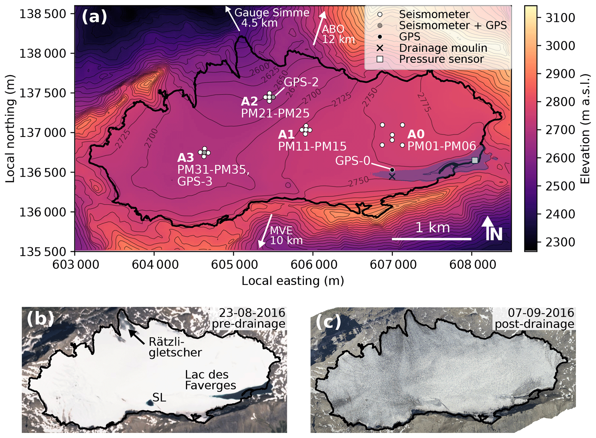
Figure 1(a) Map of the extent of Glacier de la Plaine Morte (thick black line), topography (contour lines and color-coding), and location of sensor installations (symbols). Seismic stations are numbered for each array (A0-A3) counterclockwise from 1 (north; northeast for A0) to 5 (center station). Station PM06 (lower center station of A0) was added at the end of July. The blue shaded area depicts the approximate maximum extent of Lac des Faverges with the moulin through which the drainage initiated (black “X”). The arrows indicate the direction and distance to the discharge gauge of the Simme River and to the weather stations ABO and MVE. (b) Sentinel-2 imagery (modified Copernicus Sentinel data 2019/Sentinel Hub) acquired on 23 August 2016 (day 236) with the glacier extent from (a). SL stands for supraglacial lake. (c) Orthophoto taken on 7 September 2016 (day 251) with the glacier extent from (a).
In recent years, the annual filling and subglacial drainage of an ice-dammed lake, Lac des Faverges (Fig. 1), at the southeastern rim of the glacier were observed, which increases the risk of flooding the Simme Valley to the north. In 2016, the lake reached a volume of m3, which was released within 6 d at the end of August. In addition, a smaller supraglacial lake at the southern rim (labeled “SL” in Fig. 1) formed in 2016 and drained prior to Lac des Faverges.
Our field campaign started in late April with the installation of an array consisting of five Lennartz LE3D/BH seismometers in shallow boreholes. Above 1 Hz, the sensors have a flat response to ground velocity and they were connected to Nanometrics Centaur digitizers logging data at 500 samples per second. At the end of July (day 212), we added a sixth sensor of the same type to this array. The data of this station were recorded by an Omnirecs DATA-CUBE3 at 200 samples per second. The aperture of this array was 360 m, and power supply was achieved via batteries charged by solar energy. In mid-July on days 202 to 204, we installed three additional arrays, each consisting of five stations with an aperture of 100 m. For each of these stations, we used a three-component 4.5 Hz geophone (PE-6/B manufactured by Sensor Nederland) connected to an Omnirecs DATA-CUBE3 logging ground velocity at 400 samples per second. The geophones were installed in the snowpack and later on ice (for details see Lindner et al., 2019) while the digitizers stayed at the surface to retain GPS capability. Power supply for these stations was achieved via alkaline batteries which needed to be replaced on a weekly basis. In the following, consistent with the station names, we refer to our four arrays as A0 (stations PM01–PM06), A1 (PM11–PM15), A2 (PM21–PM25), and A3 (PM31–PM35). While A0 recordings are continuous (apart from gaps due to station maintenance), recordings from the other arrays suffer from occasional power outages and frequently exhibit gaps over midnight of up to 26 min. A0, A1, and A2 stations recorded data through early September (days 250 to 252, respectively), and A3 stations were dismantled on August 23 (day 236) due to a slushy snow layer at the glacier's surface.
In addition to the seismogenic ground motion, we surveyed the (low-frequency) glacier surface motion due to ice flow and glacier hydraulics at three locations using GPS units (Fig. 1a) (2 h sampling interval after post-processing). Furthermore, we make use of the following time series: discharge in the Simme River to the north (measured ≈4 km from the terminus of Rätzligletscher), level of the outlet stream (≈1.5 km from the terminus of Rätzligletscher), and level of Lac des Faverges. Simme discharge is provided as hourly averages by Switzerland's Federal Office for the Environment, and the stream and lake level are provided through a monitoring program conducted by the municipality of Lenk and the company Geopraevent. The lake level was monitored by a pressure sensor (Fig. 1) sampling data at 10 min intervals.
3.1 Discharge
Over the course of the 2016 melt season, Lac des Faverges steadily filled (orange dashed line in Fig. 2a) and reached a maximum volume of approximately 2 million cubic meters of water at the end of August. In the evening of 27 August (day 240), a lake drainage through the moulin marked in Fig. 1a was initiated and emptied the lake basin in approximately 6 d. The moulin routed the water to the subglacial environment, and it escaped the glacier beneath the Rätzligletscher on the northern side. In the first hours of the drainage, the water escaped abruptly, since the moulin reached the bottom of the lake. This drainage phase corresponds to the peak in the discharge curve (≈25 m3 s−1) measured in the Simme Valley (blue curve in Fig. 2a and 2b). This peak discharge overwhelmed the capacities of the subglacial drainage system, which is indicated by the local ice uplift measured at all three GPS stations (Fig. 2b). As the lake level fell to the elevation of the moulin inlet, the direct connection between moulin and lake became disrupted. Subsequently, the lake connected to the moulin through a supraglacial channel which steadily incised deeper into the ice but slowed down the drainage (6–11 m3 s−1). The exact transition time to this state is unknown but was within the first day of the drainage initiation.
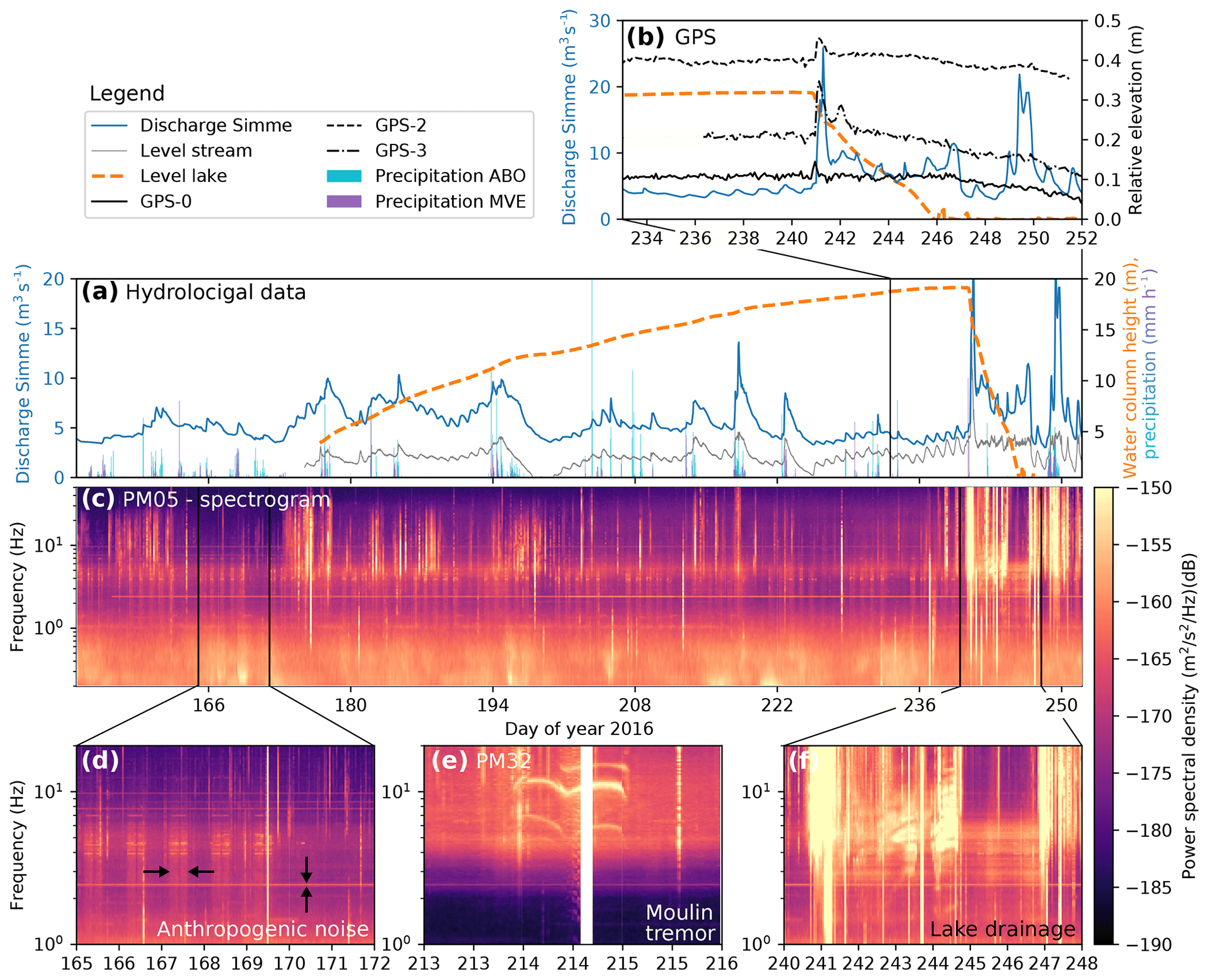
Figure 2(a) Hydrological data recorded in the vicinity of Glacier de la Plaine Morte: discharge of the Simme River measured in the Simme Valley (blue curve; ≈4 km line of sight from the glacier terminus), level of the Trüebbach stream (gray curve; ≈1.5 km from glacier terminus), height of the water column in the lake above the pressure sensor (orange dashed), and precipitation at stations ABO and MVE (blue and purple bars; 12 km north and 10 km south of the glacier, respectively). (b) Discharge and lake level for the drainage period (same as a) and the vertical displacement of three GPS units (black lines). (c) Spectrogram of station PM05 for the same time period shown in (a). (d) Zoom of the spectrogram in (c) showing anthropogenic noise. (e) Zoom of a spectrogram of station PM32 showing moulin resonances. The white bar indicates a data gap due to station maintenance. (f) Zoom of the spectrogram in (c) showing the lake drainage. Note that data used to calculate the spectrograms are not corrected for the instruments' phase responses.
Discharge magnitudes similar to those of the lake drainage period were also measured in the Simme River prior to the lake drainage (three peaks on days 213–225) and after the lake drainage (days 248–252). Most of these discharge peaks can be linked to rainfall events having a shorter duration than the lake drainage (precipitation data are provided by the Switzerland's Federal Office of Meteorology and Climatology MeteoSwiss). Since precipitation affects the entire catchment above the gauging station (more than 4 times the glacier surface area), these precipitation-related discharge events need to be interpreted with caution because part of the measured discharge at those times may be due to water flowing outside of the glacier. In general, however, the similarity of the discharge curve and the stream level height measured close to the glacier terminus suggests that Glacier de la Plaine Morte is the main contributor to the discharge measurements. In addition to the drainage of Lac des Faverges, a smaller supraglacial lake at the southern rim of the glacier (labeled SL in Fig. 1b) was observed to drain via a supraglacial canyon routing water to moulins. A field visit on day 239 revealed that the lake was draining, but the time of the drainage initiation was not witnessed.
3.2 Seismic tremors
Figure 2c shows a spectrogram for station PM05. Recent studies suggest that water routing in subglacial conduits generates seismic tremors observable in the frequency range 1–10 Hz (Bartholomaus et al., 2015; Gimbert et al., 2016). In this frequency range, however, we observe several signals of anthropogenic origin. These include a diurnal signal from Monday to Friday with sharp onset and decay times, a monochromatic signal visible as a spectral line at roughly 2 Hz starting from day 156, and most likely also the diffuse band centered around 5 Hz (Fig. 2c–d). Regarding glacier seismicity, we identify a harmonic moulin tremor with three prominent frequencies which indicate resonant modes in the water column, similar to those in Roeoesli et al. (2016) (Fig. 2d). During the lake drainage, the signal strength is increased for frequencies greater than 1 Hz, and we observe high-frequency tremors (>3 Hz) during the drainage initiation (Fig. 2c and e).
To better distinguish the seismic signal contributions, we investigate the wave field in more detail. For this purpose, we calculate 3-D particle motion polarization attributes following Koper and Hawley (2010). This approach is based on an eigen-decomposition of the spectral covariance matrix containing the power and cross spectra of a single three-component station (Vidale, 1986). One of the polarization attributes, the difference in phase between the vertical component and the principal horizontal component, ϕVH, allows us to distinguish between different wave types. In particular, the elliptical particle motion of a Rayleigh wave is caused by a 90∘ phase shift between vertical and horizontal ground motion and distinguishes it from other wave types. To calculate the polarization attributes, we use the freely available toolbox hosted on the IRIS web page (http://ds.iris.edu/ds/products/noise-toolkit/, last access: November 2019) with the default parameters and processing steps (including instrument response removal; see Koper and Hawley, 2010). Figure 3 shows probability density functions of ϕVH for a station of each array. Consistent with an elliptical particle motion in the vertical–radial plane associated with Rayleigh wave propagation, ϕVH clusters around ±90∘ in the frequency range 8.5–12 Hz for all four stations shown. Below 8.5 Hz (6 Hz for station PM33), i.e., frequencies where anthropogenic noise is evident, clustering around ±90∘ indicative of Rayleigh waves is not present or only in narrow frequency bands (e.g., 4–5 Hz for station PM05). We do not find a difference in the polarization results prior to and during the lake drainage, though the short duration of the drainage process hinders a detailed comparison by means of a statistical representation as shown in Fig. 3.
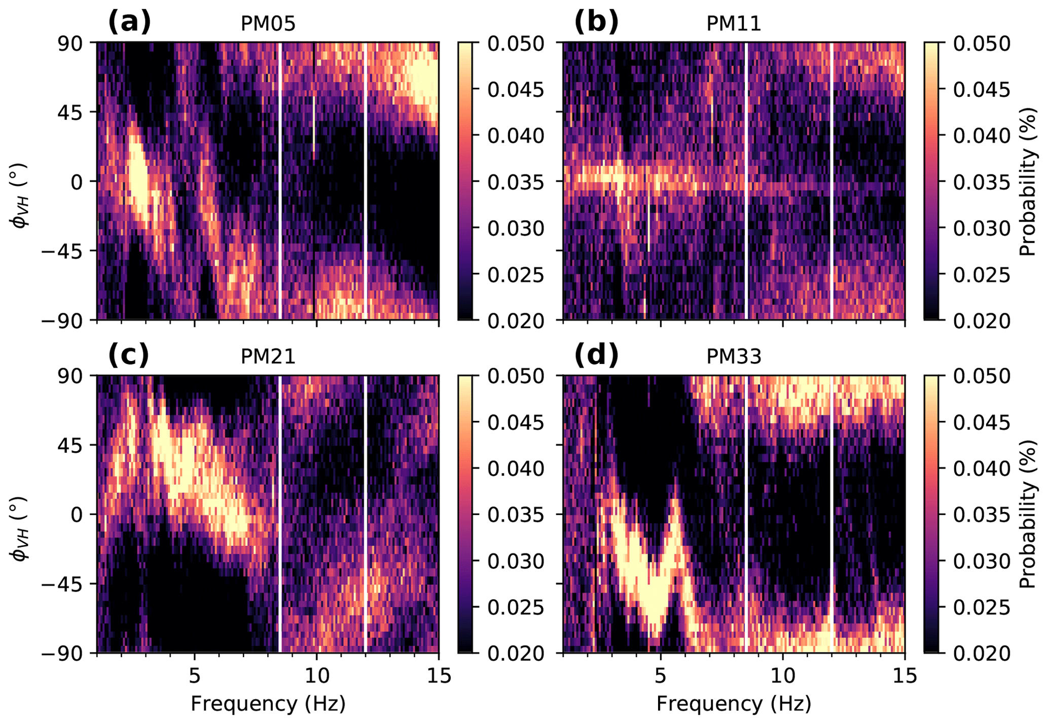
Figure 3Probability density functions for the phase difference between the vertical component and principal horizontal component. Probabilities are calculated for the time period 22 July 2016 to 6 September 2016 (23 August 2016 for station PM33) and bins of 5∘ width. The results are shown for one station of each array: (a) PM05, (b) PM11, (c) PM21, and (d) PM33.
Since the continuous recordings below ≈8.5 Hz are contaminated by anthropogenic noise with a complex wave-type signature, we chose to analyze the frequency range 8.5–12 Hz in the context of glacial hydraulics. This frequency range is dominated by Rayleigh wave energy, which facilitates the tremor location analysis in the next section. To investigate possible correlations between discharge and seismicity for the 8.5–12 Hz range, we calculate the tremor amplitude, or median absolute ground velocity, for the vertical component of ground velocity as described in Bartholomaus et al. (2015). Figure 4 shows the resulting time series for a station of each array along with the discharge recordings. Prior to the lake drainage, variations in tremor amplitude are weak but follow the discharge curve (e.g., days 213–225). In the 4 d preceding the lake drainage, the daily melt cycle due to high temperatures is visible in both the discharge time series and the tremor amplitude curves. During and after the lake drainage, tremor amplitudes are increased and show stronger variations than prior to the lake drainage. From Fig. 4b we note that PM21's tremor amplitude correlates with discharge particularly well.
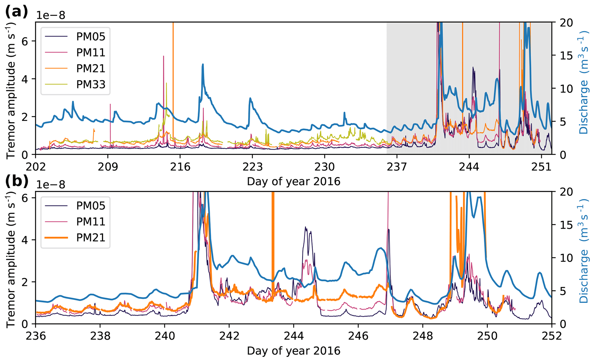
Figure 4(a) Tremor amplitude (8.5–12 Hz) time series for a station of each array (thin colored lines) and discharge (thick blue line). (b) Zoom of the gray shaded area in (a).
3.3 Icequake activity
To investigate the interplay of glacial hydraulics and icequake activity on Glacier de la Plaine Morte, we build on the results of Lindner et al. (2019). This study focuses on ice-fracturing events (Walter et al., 2009) to investigate azimuthal anisotropy of seismic wave propagation, but the events are also useful to study fracturing associated with glacial hydraulics, e.g., during outburst floods (e.g., Roux et al., 2010). Lindner et al. (2019) detect icequakes by applying a short-term average and long-term average (STA–LTA) trigger (Allen, 1978) on bandpass-filtered data (10–20 Hz for A1, A2, A3; 7–15 Hz for A0), require at least three stations of an array to trigger concurrently, and disable the trigger for 3 s after a detected event to avoid overlapping event windows (for parameter details see Lindner et al., 2019).
From the event catalogs from each array, we calculate the icequake detection rate in events per hour. Figure 5 shows that icequake activity is often increased during discharge peaks, though not always. Given the correlation between tremor amplitude and discharge (Fig. 4), this implies that the tremor amplitude in turn is also correlated with the icequake rate (see blue arrows in Fig. 5). In addition, we identify times when correlation of the tremor amplitude with the icequake rate is higher than with discharge (red arrows in Fig. 5). These features correspond to icequake bursts lasting on the order of hours but less than a day. Maximum detection rates are 352, 314, 172, and 20 icequakes per hour for A0, A1, A2, and A3, respectively. For A0, this corresponds to 5.87 icequakes per minute and thus almost 18 s of disabled trigger per minute (trigger disabled for 3 s after event). This suggests that our results are a conservative estimate of icequake occurrence. We note that especially those arrays with high icequake rates (A0 and A1) suffer from icequake contaminated tremor amplitudes. This contamination might be reduced by choosing different window lengths for the calculation of the tremor amplitude, but investigating this matter is beyond the scope of this study.

Figure 5Icequake detections per hour for all arrays (gray bars; see text for details) and the discharge curve of the Simme River (blue line). The black, magenta, orange, and green lines (from top to bottom) are the tremor amplitude curves shown in Fig. 4. Note the different tremor amplitude scaling between the two panels. Blue arrows indicate times where the tremor amplitude correlates with both discharge and icequake rate. Red arrows indicate times where the tremor amplitude correlates with icequake rate only. The black dashed rectangle indicates times, where three of five A2 stations tipped over due to diminishing snow cover. The icequake rates in this interval need to be taken with caution.
For further insights into the glacial hydraulics, we consider the icequake source locations as determined from plane-wave beamforming (for details see Lindner et al., 2019). Plane-wave beamforming enables us to determine the back azimuth of an incident signal with an array of sensors. Its generalization to epicentral coordinates will be introduced in Sect. 4.
Figure 6b shows the icequake detections of A1 as a function of focal time and source back azimuth. Some peaks in discharge, e.g., on day 222, are accompanied by fracturing at various source back azimuths. Since A1 is in the glacier's center and icequakes arrive from various back azimuths, this suggests that these discharge events affect large portions of the glacier. Other events, e.g., the melt cycle in the days prior to the lake drainage, are accompanied by more localized seismicity at back azimuths of 50–100∘ only. The latter is also the case for the ≈24 h preceding the drainage initiation, where the seismicity at the back azimuth towards the main drainage moulin is increased. We also detect icequakes at this back azimuth earlier, but activity is not sustained and back azimuths do not focus on the moulin. With the onset of the lake drainage, fracturing occurs at various back azimuths with a focus on the lake basin. After the drainage, fracturing is predominantly confined to the lake basin as well.
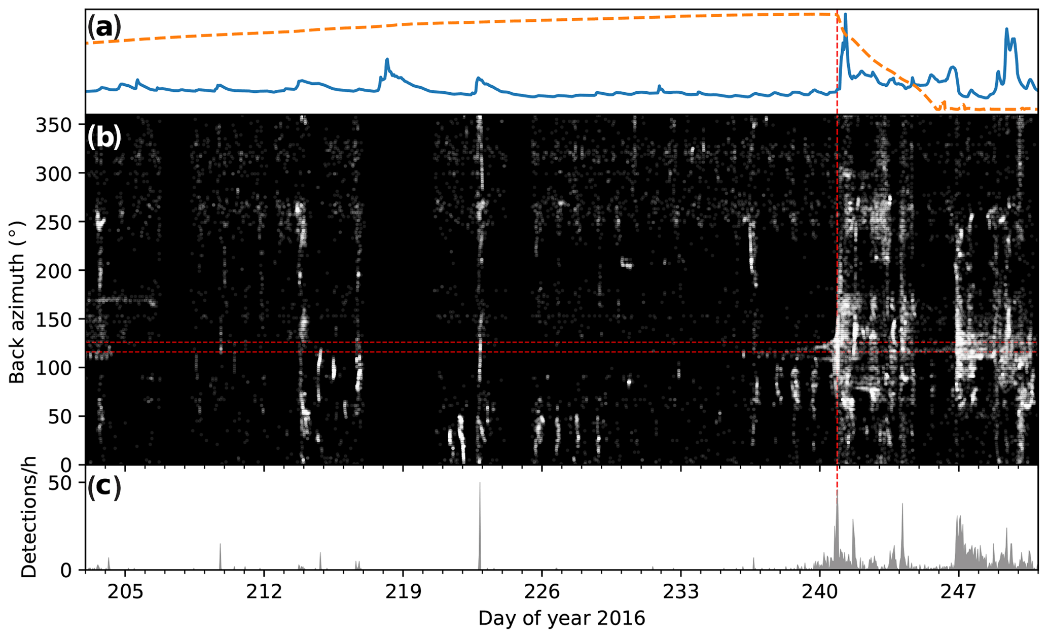
Figure 6(a) Discharge and lake level (same as in Fig. 2). The vertical red dashed line indicates the drainage initiation. (b) Detected icequakes at A1 as a function of time and source back azimuth (white dots on black background). Icequake clustering in both time and back azimuth is visible as bright white spots. The two horizontal red dashed lines indicate the back azimuth from the array center to the main drainage moulin ±5∘. (c) Icequakes per hour in the back-azimuth range marked with the two horizontal red dashed lines in (b).
We note that STA–LTA detection thresholds might be affected by changes in the background noise level (Walter et al., 2008), resulting in biased event detections. However, since our focus is on periods with high discharge or strong melting (as in the hours prior to the drainage initiation) in which trigger sensitivity is typically decreased, we argue that our results are robust.
4.1 Matched-field processing
To locate the sustained tremor sources, we apply matched-field processing (MFP; Baggeroer et al., 1993) to our four seismic arrays. MFP measures signal coherence of a phase across an array of receivers and matches it against a synthetic wave field computed for a point source and a velocity model. By testing various source positions and velocity models for the synthetic field, a grid search finds the combination of source position and velocity model which best matches the measured coherence across the array. The result is the most likely source location and velocity model. Allowing near-field point sources, and hence circular wave fronts, MFP is a generalization of the conventional plane-wave beamforming approach used to determine the slowness and back azimuth of incoming waves (Rost and Thomas, 2002). In case the distance of a source to the array is greater than 2 to 3 times the array aperture, the circular wave front approach converges towards a plane-wave solution (Almendros et al., 1999). For MFP, this implies that far-field sources allow a back-azimuth estimate only (as is the case for plane-wave beamforming), while near-field sources can be associated with epicentral coordinates. We leverage this to locate tremor sources, some of which are in the arrays' near field as we show in the following.
The workflow for MFP is as follows (for a more detailed introduction, see, e.g., Corciulo et al., 2012). From the time-domain ground-velocity recordings of N receivers grouped to an array, the discrete Fourier transforms at some angular frequency of interest ω are calculated. The resulting complex frequency-domain values are arranged to form a column vector d(ω) of length N. From this column vector, the cross-spectral density matrix K(ω) is calculated as
where † denotes the complex conjugate transpose operation. Note that the diagonal elements of K(ω) are the autocorrelation values of the N receivers at ω, while the off-diagonal elements are cross-correlation values of receiver pairs. Both autocorrelation and cross-correlation are discrete values associated with angular frequency ω, and the latter represent average phase delays between two receivers at ω. The synthetic field at ω is calculated for each of the j=1, …, N receivers as
where i is the imaginary unit, rj is the source–receiver distance of the jth receiver, and c is the phase velocity of the velocity model, which is constant in the case of a homogeneous ice body. Note that this representation focuses on phase information and disregards amplitude information. For j=1, …, N, the complex values are arranged to form the synthetic column vector (equivalent to the data vector d(ω)), and phase matching is achieved via the conventional Bartlett processor (Baggeroer et al., 1993),
or via a high-resolution MFP method, i.e., the minimum variance distortionless response (MVDR) beamformer (Capon, 1969; Corciulo et al., 2012),
where K−1 is the inverse of the cross-spectral density matrix K. In case the incoherent noise power is small relative to the power of the signal of interest, the MVDR processor is capable of estimating the source location and the velocity beneath the array with higher resolution than the Bartlett processor (Capon, 1969). Note that there is a trade-off between high-resolution and robustness; i.e., in contrast to the MVDR processor, the Bartlett processor might still produce meaningful results if the incoherent noise power is increased.
4.2 Single-array results
To investigate the spatial variability of tremor sources across Glacier de la Plaine Morte, we apply MFP to all four arrays individually. For this purpose, we use a sliding window of 15 min length (without overlap) over the entire data set to also resolve temporal variations. Each of these 15 min segments are processed as follows. To suppress incoherent noise, we calculate the ensemble average of K(ω) at discrete frequencies, using a 10 s sliding window with 50 % overlap (e.g., Corciulo et al., 2012). The overlap criterion yields a total set of 179 windows over which we average. In the frequency range of 8.5–12 Hz, the results from our polarization analysis (Fig. 3) suggest Rayleigh waves whose amplitude is correlated with discharge. For this reason, we calculate the MFP results in 0.1 Hz steps and average over the frequency range of 8.5–12 Hz. For the velocity c in Eq. (2), we use the local Rayleigh wave velocities which are 1600, 1800, 2200, and 1600 m s−1 for arrays A0, A1, A2, and A3, respectively (Lindner et al., 2019). In the spatial domain, we apply a grid search over the entire glacier surface and its surroundings (assuming a horizontal plane) to calculate the rj values in Eq. (2) with a spacing of 25 m in the x and y directions. Figure 7a shows the spatial clustering of the MFP results from all available time windows using the MVDR processor. The picked and shown epicenters are associated with the maximum BMVDR value of all tested coordinates.

Figure 7(a) MFP locations (MVDR processor) over the frequency range 8.5–12 Hz assuming Rayleigh wave velocities (colored dots). Each dot is the result obtained for a 15 min window. The thick black line indicates the glacier margin in 2015, the black triangles the locations of the seismic stations, and the gray dashed circles the distance of twice the array aperture from the array center. The black “X” symbols indicate positions of moulins identified from orthophotographs (by swisstopo, SWISSIMAGE). The red “X” marks the position of the lake drainage moulin. Labels of type A0-2 refer to dominant source clusters discussed in the text. (b–e) Temporal variation in back azimuth and distance of the tremor source locations (colored dots) from (a) as seen from the array centers of A0, A1, A2, and A3. The gray line depicts the discharge curve measured in the Simme Valley for reference.
4.2.1 Array A0
For array A0, three dominant clusters are discernible. Prior to the lake drainage, tremors locate to the north close to the array (Fig. 7, labeled as A0-1) with a few exceptions at high discharge where tremors approach the array from the west. At the drainage initiation, no clear source region can be identified, but with the onset of the drainage, the source locations cluster near the main drainage moulin (A0-2). This signal remains stable for almost 4 d before switching again to the source in the north until the end of the drainage. After the lake drainage, the MFP locations cluster predominantly around another moulin in the lake basin which was identified from a high-resolution (0.25 m pixel size) orthophotograph taken on 7 September (by swisstopo, SWISSIMAGE) just after the drainage (A0-3). All three source clusters are located within twice the array aperture, and two of them coincide with moulin locations. For this reason, we argue that the MFP locations are robust, event though uncertainties in epicentral distances increase with distance to the array (Walter et al., 2015).
4.2.2 Array A1
Prior to the lake drainage, MFP applied to A1 reveals source clustering towards A2 and the small glacier tongue (A1-1). However, on day 232 concurrent with a small peak in discharge and in the 5 d prior to the lake drainage, another source southwest of the array becomes active (A1-2). In both cases, epicentral distances are not well resolved, which becomes apparent in the elongated clustering in Fig. 7a and in the short-term fluctuations of the epicentral distance in Fig. 7c. In addition, many source location estimates are beyond the doubled-aperture distance, meaning that the curved wavefront used in MFP converges towards a plane wave which allows back-azimuth estimates of the incoming waves only (Almendros et al., 1999). During and after the lake drainage, A1 receives signals from two distant sources acting concurrently. One is similar to the dominant source prior to the lake drainage (back azimuth ≈320∘) but appears to be associated with slightly increased back-azimuth (5–10∘) and distance estimates. The other source originates in the lake basin direction (A1-3) where two moulins are located, which also coincide with A0 source locations at the same time.
4.2.3 Array A2
A2 shows less variation than A1 and the source clustering suggests a close tremor source to the northwest of the array in the direction of the small glacier tongue (A2-1). During and after the lake drainage and similar to A1, this source seems to wander slightly farther away towards the north (back-azimuth increase of 5–10∘). Again, however, epicentral distance is not well resolved. In some instances and mainly concurrent with discharge peaks, additional signals arrive from a more distant source west of the array (A2-2).
4.2.4 Array A3
Tremor signals observed at A3 mainly arrive at the array from the west with back azimuths in the range of approximately 250–285∘ (A3-1). The epicentral distances of these sources cannot be constrained but their back-azimuth points towards a region of the glacier where several moulins are located. Some of them have a sinkhole-like structure tens of meters in diameter and are stationary over decades (Huss et al., 2013; GLAMOS, 2018). We also note that a military radar facility is located at a back azimuth of approximately 275∘ and a distance of around 2 km from the array center, whose operation cannot be excluded as a noise source for A3. Another tremor source is located southwest at a back azimuth of around 230∘ (A3-2). This source clusters closer than twice the array aperture, is collocated with the position of a moulin identified from orthophotographs, and appears to be active during peak discharges.
4.2.5 Discussion
We also test the MVDR results for plausibility by comparing them to the solutions obtained by using the Bartlett processor (Eq. 3). Even though these results were obtained for a smaller spatial grid in order to save computation time, both processors yield similar results. In addition, we also test the robustness of our results by (apart from testing a grid of coordinates) also allowing a grid search over phase velocity from 1500 to 3500 m s−1 in 50 m s−1 steps. Compared to the MVDR–Rayleigh results (Eq. 4), both the back azimuth and the epicentral distances scatter more broadly, but the general source distribution stays similar. The velocities for which the Bartlett results are maximized are systematically higher than the Rayleigh wave velocities used previously, especially for A2 (median of approximately 2800 m s−1 versus 2200 m s−1 for Rayleigh waves). However, the average Bartlett maximum is increased only marginally (0.86 for Bartlett–Rayleigh MFP versus 0.88 for Bartlett MFP with velocity grid search), which indicates that there is a trade-off between epicentral distance and velocity. Here, we note that Walter et al. (2015) find quickly growing uncertainties in epicentral distance estimates of icequakes with distance from the array center. These uncertainties in the source locations also evident in Fig. 7 are further discussed in Appendix A.
The polarization analysis (Fig. 3) suggests that Rayleigh waves are the dominant wave type, though we cannot exclude body wave contributions. Such a contribution could increase the measured apparent velocity due to the higher subsurface velocities of P-waves compared to Rayleigh waves. S-wave velocities in the ice and bedrock (Lindner et al., 2019) are too low to explain the measured velocities at A2. The fact that the median velocities are consistently closer to the expected Rayleigh wave velocity than to the P-wave velocity in ice (>3600 m s−1, Podolskiy and Walter, 2016) confirms the polarization results, i.e that Rayleigh wave propagation is dominant.
4.3 Multi-array results
To further constrain the tremor source locations, we stack the results obtained from the different arrays. Following the argumentation in the previous section, we continue to focus on Rayleigh waves and consider the MFP results obtained for the MVDR processor on the entire spatial domain used for the grid search. Figure 8 (left column) shows the results for a 15 min window on day 214 during a peak in discharge caused by precipitation. As reported in the previous section, A0 sees a persistent source to the north of the array, A1 and A2 point towards the glacier tongue, and A3 points toward the (south)west. For A3, however, a secondary lobe of the MVDR output is visible, which points to the glacier tongue as well. We combine the information from different arrays by stacking the MVDR grid-search results, which shows high MVDR values in regions where multiple arrays locate signals. The stacking allows triangulation and confirms that the main tremor source is in the region of the glacier tongue (Fig. 8, left column). We tested other time windows and found that the depicted situation is representative for the pre-drainage period which appears stable with little excursions to other source regions (see Fig. 7b–e). With the onset of the drainage, the tremor source locations change, as shown in Fig. 8 (right column). The depicted situation shows the result for a 15 min window on day 243 roughly 55 h after the drainage initiation. A0 now locates the tremor signal south of the array and A1 points towards the southeast with a secondary lobe pointing to the glacier tongue. A2 again points towards the glacier tongue with less scatter compared to Fig. 8, left column. As discussed in the context of Fig. 7b–c, A1 (secondary lobe) and A2 back azimuths are slightly increased compared to the pre-drainage period. Stacking the results from A0, A1, and A2 again (A3 has no data) shows two source regions, the glacier tongue and the main drainage moulin.
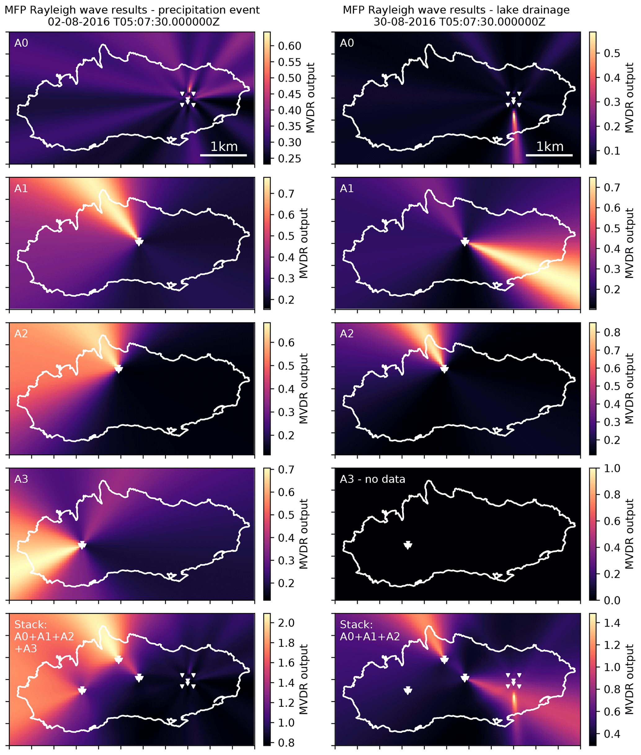
Figure 8MFP results obtained using the MVDR processor and Rayleigh wave velocities. Shown are the results for the single arrays (rows 1–4) and a stack of the arrays (last row). The left column shows the results of a 15 min window on day 214 during a peak in discharge caused by precipitation. The right column depicts the results of 15 min windows during the lake drainage on day 243. Exact times are given on top of the plots. The spacing of the ticks on the x and y axes is 500 m (see also Fig. 1).
To facilitate the interpretation and discussion of the recorded tremors in the context of glacier hydraulics, we first consider the theoretical geometry of subglacial drainage. Figure 9 shows the likely flow paths of subglacial drainage calculated from the hydraulic potential (Shreve, 1972) for two scenarios: (i) englacial water pressures are equal to half of the ice overburden pressure and (ii) englacial water pressures are equal to the ice overburden pressure (flotation). Details on the calculation of the hydraulic potential and the shown upstream area distributions which indicate the spatial extent of hydraulically connected areas, i.e., likely subglacial flow paths, can be found in Appendix B. Consistent with field observations, both results suggest that almost all water drains through a main outlet beneath Rätzligletscher to the north. At flotation, a second outlet a few hundred meters to the west of the glacier tongue is visible. In both cases, the roots of the dendritic network associated with the main outlet are located in both the eastern and western portions of the glacier.
5.1 Tremor composition
The results from our tremor analysis demonstrate that the recorded seismic wave field on timescales beyond those of discrete single events is generated by various processes. Apart from cryo-seismicity, we observe signals of anthropogenic origin. The diurnal signal occurring on working days only (Fig. 2c; also reported in Preiswerk and Walter, 2018), originates to the south of Glacier de la Plaine Morte (determined by plane-wave beamforming), likely in the Rhone valley where industry is located. The frequency range of anthropogenic noise (e.g., Anthony et al., 2015) often overlaps with the discharge–tremor band, meaning that glacioseismological data need to be analyzed carefully in glaciated regions with anthropogenic activity such as the European Alps to avoid misinterpretation. This also holds in the absence of anthropogenic noise, since our data reveal that tremors may be generated by different aspects of glacier hydraulics at the same time. We identify tremors which are dominated by energy released through ice fracturing (A0 and A1), are located at moulin locations (A0 and A3), or exhibit a characteristic frequency signature of moulin resonances (A3) and thus obscure turbulent-flow tremors. However, at A2, we argue that the recorded tremors are generated by subglacial water routing for the following reasons: (i) the tremor amplitude correlates with the discharge curve (Fig. 4) and (ii) MFP shows a persistent source in the region of the glacier tongue (Fig. 7a), from where (iii) the main glacier outlet emerges (Fig. 9). We note that subglacial water routing in turn can generate tremors both via pressure fluctuations in turbulent flow and via impact events from bed load sediment transport (Gimbert et al., 2014, 2016). Recent studies (Bartholomaus et al., 2015; Gimbert et al., 2016) typically separate the two processes by frequency at around 10 Hz; thus the frequency range associated with our results (8.5–12 Hz) may contain both processes. Even though we cannot exclude that bed load significantly contributes to total seismic power, we see evidence for water tremors being the dominant source for the following reasons. (i) The frequency ranges are controlled by various parameters (channel-to-station distance and channel apparent roughness among others) also permitting turbulent-flow tremors above 10 Hz (Gimbert et al., 2014). (ii) Ice flow of Glacier de la Plaine Morte is negligible (<1 cm d−1 at A2, not shown), resulting in little sediment production by abrasion (Hallet, 1979), which we expect hinders bed load tremor generation. (iii) The A2 tremor–discharge scaling as discussed later tends to follow the drainage-regime predictions for water tremors without evidence for a hysteresis due to sediment flushing (e.g., Gimbert et al., 2016). Apart from various tremor sources, we finally note that the tremors are composed of different wave types, further increasing the complexity of the tremor signal.
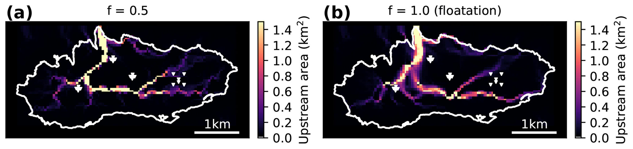
Figure 9Upstream area distributions calculated from the hydraulic potential (see text for details). (a) Solution obtained for (spatially uniform) water pressures of half the ice overburden pressure. (b) Solution obtained for (spatially uniform) water pressures equaling the ice overburden pressure. The white triangles indicate the positions of the seismic stations.
5.2 Temporal evolution of the drainage system
Figure 7b–e shows that the tremor locations change over time. Since icequake tremors typically last on the order of hours (Fig. 5) but the inferred back azimuths of sources stay stable on the order of days to weeks, we attribute the dominant source locations to moulin tremors and subglacial water routing. At the end of July (when the deployment of all sensors was completed), A1 and A2 tremor sources locate towards the glacier tongue, and A3 tremor sources locate in the region to the west of the array where multiple moulins are located. In addition, we note that seismic tremors are likely generated by efficient channelized subglacial flow (Gimbert et al., 2016) and that the moulins in the vicinity of A3 seemed to evacuate meltwater without the buildup of supraglacial lakes or reservoirs. We therefore suggest that the left branch of the upstream area distributions in Fig. 9, or more general the western and northern part of the glacier, had an efficient and channelized subglacial drainage system. According to Fig. 7c, this configuration stayed stable until the end of August (day 236). At the same time, A0 saw a persistent source to the north whose origin remains elusive. A potential explanation for this source could be another moulin feeding the upstream area branch (Fig. 9) originating in the northeast of the glacier. However, neither the observations from our regular station visits nor the orthophotograph show evidence for a moulin in the area of A0. Starting on day 236, A1 points toward the southwest (Fig. 7), and we attribute this source to the drainage of the smaller supraglacial lake (SL in Fig. 1b). With the onset of the drainage of Lac des Faverges, tremors from the lake basin become dominant (A0 and A1), suggesting that the eastern part of the glacier has an efficient connection to the drainage system, as tremors are expected to originate from channelized flow (Gimbert et al., 2016). Combining this information with the theoretical pattern of subglacial water routing (Fig. 9) suggests that the seismic tremors reveal a gradual “up-glacier” (along the main branch in Fig. 9 from north to south to east) evolution of an efficient channelized drainage system as the melt season progresses. This matches both the field observations (first SL connects to the drainage system, then Lac des Faverges) and the theory of subglacial channel evolution throughout a melt season (Werder et al., 2013).
While subglacial channel evolution is typically described through the competing mechanisms of melting and ice creep (Röthlisberger, 1972), our results show that fracturing can play an important role under specific flow scenarios. We find that icequake activity in the lake basin precedes the drainage onset by several hours (Fig. 6). In combination with a lake reservoir which pressurizes the void spaces and the englacial environment, we suggest that hydrofracturing (e.g., Van Der Veen, 1998; Roberts et al., 2000) drives the drainage initiation. Since no sustained seismicity in the lake region is detected prior to that, this highlights the potential of passive seismic monitoring for early warning of glacier-dammed lake outburst floods. Apart from the lake drainage, other discharge peaks are accompanied by fracturing as well (Figs. 5 and 6). However, we note that elevated strain rate resulting from water-enhanced basal sliding may give rise to icequakes as well (Podolskiy et al., 2016).
5.3 Drainage regime
5.3.1 Theory
Water flow through ice-walled conduits is driven by the hydraulic pressure gradients along the conduits. Along the channel walls, frictional heat enlarges the channels. At the same time, ice creep closes the conduits in the case where the ice overburden pressure exceeds the water pressure in the conduit (Röthlisberger, 1972). These two counteracting processes result in a temporal evolution of conduit radius and water pressure in the conduit. Recently, Gimbert et al. (2016) suggested that pressure fluctuations due to turbulent flow in subglacial conduits can generate seismic tremors whose power scales with discharge according to the drainage regime. Gimbert et al. (2016) derive two end-member scenarios for which the relative seismic power Prel and relative discharge Qrel (with respect to some reference state) are related through a power law but with a different scaling exponent.
- i.
Varying hydraulic pressure gradient and constant hydraulic radius, implying . As defined in Gimbert et al. (2016), changes in the hydraulic pressure gradient are caused by variations in the water pressure p along a conduit, i.e., , where x is the distance along the channel. Such a situation is schematically depicted in Fig. 10, where, for instance, the diurnal melt cycle causes hydraulic head variations in a moulin without changes in the hydraulic radius of the conduit. At some distance from the moulin, at the glacier snout, water constantly flows at atmospheric pressure. As the hydraulic head in the moulin varies, this results in pressure-gradient changes in the subglacial conduit implying . This drainage regime is expected to dominate in filled subglacial conduits which do not adjust their hydraulic radii fast enough to accommodate discharge changes. We expect that this occurs, for example, for strong daily melt variations in the early melt season (when the capacity of the conduits is still limited) or for rapid water input due to a sudden lake drainage.
- ii.
Varying hydraulic radius and constant hydraulic pressure gradient, implying . As the hydraulic radius of a conduit is defined as its cross-sectional area divided by the wetted perimeter, both changes in the water level of a conduit operating under atmospheric pressure and the cross section of a fully filled conduit result in variations in the hydraulic radius (Fig. 10). For instance, subglacial water routing at atmospheric pressure is predicted to be revealed by the power law as the wetted perimeter can vary without geometrical changes in the subglacial conduits. The same scaling relationship holds for filled conduits, in case melt enlargement and creep closure of channels dominate over changes in the pressure gradient.
Gimbert et al. (2016) also derived solutions for the relative hydraulic pressure gradient Srel and the relative hydraulic radius Rrel (again with respect to some reference state) as a function of observed Prel and Qrel, given as
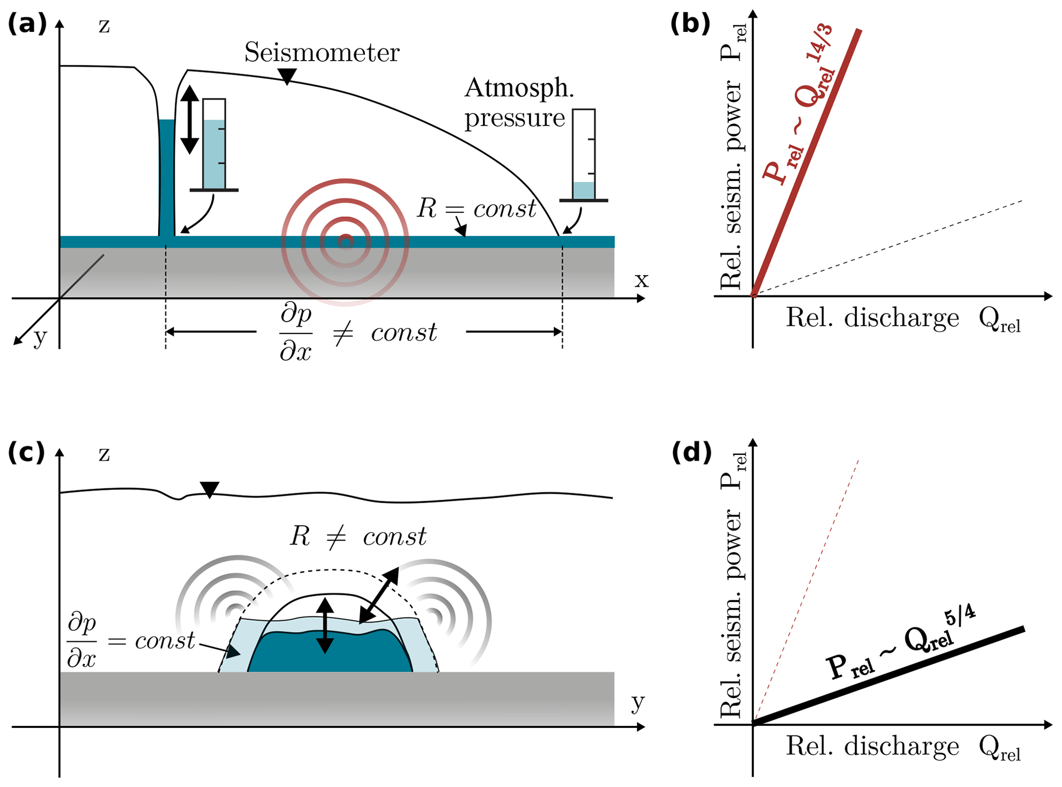
Figure 10Interpretation of the theory of Gimbert et al. (2016) relating seismic power to discharge. (a) Cross section through a glacier parallel to the flow direction. The hydraulic head in the moulin varies due to, for example, the daily melt cycle. The hydraulic radius of the subglacial conduit is constant. As the water routing at the glacier snout occurs at constant atmospheric conditions, a pressure gradient in the subglacial conduit is present. (b) For such a configuration of varying hydraulic pressure gradient (and constant hydraulic radius) the relative seismic power is predicted to scale with the relative discharge (relative to some reference state) to the power of 14∕3. (c) Cross section perpendicular to the flow direction. The hydraulic radius of a subglacial conduit varies through a change in water level or through changes in the cross-sectional area due to frictional melting or creep closure. The pressure gradient is assumed constant. (d) For such a configuration of varying hydraulic radius (at constant hydraulic pressure gradient), the relative seismic power is predicted to scale with the discharge to the power of 5∕4.
5.3.2 Observations
At A2, we observe tremors due to subglacial water flow beneath Rätzligletscher. Knowing the source locations of subglacial tremors allows us to apply the tremor–discharge relationships to a specific area. If the source locations are not known, the tremor–discharge scalings provide an integrated view over the surroundings of the seismic measurements, whereas the locations presented in Fig. 7 allow us to investigate glacier hydraulics at a specific point, i.e., beneath Rätzligletscher. As Rätzligletscher accommodates the main outlet, we argue that discharge measured in the Simme Valley is representative for water routing at the measured A2 tremor locations. Furthermore, we expect that the number of conduits close to the outlet stays constant. Both assumptions favor the successful application of the tremor–discharge relationships.
Figure 11 shows the scaled seismic power Prel (square of the tremor amplitude) versus the scaled discharge Qrel (using the minimum discharge value and its associated seismic power for scaling) on a log-log plot (for details see Appendix C). In this representation, the slope equals the exponent x of , where the black lines indicate discharge routing accommodated by hydraulic radius adjustment () and the red lines discharge routing accompanied by variations in pressure gradient ().
Figure 11Tremor–discharge scaling of station PM23. (a) Tremor amplitude (black) and discharge curve (colored) for the pre-drainage period. (b) Scaled seismic power as a function of the scaled discharge (see text for details) on a log-log plot. Color-coding corresponds to the colors in (a). Red and black lines are the drainage-regime predictions of Gimbert et al. (2016) and indicate discharge routing through variations in the hydraulic pressure gradient and variations in the hydraulic radius, respectively (see legend). (c) Distribution of slopes (and thus exponents) calculated from the log-log representation of two adjacent samples each. Black and red bars again show the expected exponents for the two drainage regimes (see legend in b). (d–f) Same as (a)–(c) but for the drainage period.
In the pre-drainage period (Fig. 11a), the power–discharge representation shows a general trend towards radius-adjusting conduits. This is also revealed by the x-exponent distribution (upper right in Fig. 11a) obtained by calculating the slopes between two adjacent samples. This in turn implies that pressure-gradient adjustment occurs rarely and on short timescales only. Such a system is indicative of a well-established, channelized drainage system evacuating water efficiently without significant pressurization. We find such a configuration on Glacier de la Plaine Morte, where the source region of the tremors corresponds to the main trunk of an arborescent drainage network (indicated by the upstream area distributions). However, for the approximately 10 d preceding the drainage but in particular for the last 4 d of this time span with a pronounced diurnal melt cycle, the data suggest pressure-gradient adjustments (yellow dots). This indicates that the capacity of the conduits cannot yet accommodate the water from the melt events without pressurization.
Figure 11b shows the power–discharge scaling for the drainage period. At the drainage onset, the data points scatter along the pressure-gradient adjustment prediction (black dots). Subsequently, after a more chaotic phase associated with clockwise hysteresis, the data reveal hydraulic-radius adjustments during most of the drainage period (purple and orange dots), which is again followed by pressure-gradient adjustments at the end of the drainage (yellowish dots).
To investigate these observations in more detail, we consider the evolution of the hydraulic pressure gradient and the hydraulic radius as calculated from Eqs. (5) and (6), respectively. In Fig. 12, we compare Rrel and Srel to the measurements of the lake level and the ice surface uplift, which also provide constraints on the drainage hydraulics. In addition, the pictures of the automatic camera provide an estimate of the time when the lake basin was empty. As already inferred from Fig. 11, the diurnal melt cycles prior to the drainage cause pressure-gradient variations while the hydraulic radius changes little. In this phase, the daily peaks of the pressure gradient occur around the time of maximum daily discharge. At the onset of the lake drainage in the evening of day 240 as the lake level starts to drop (gray dashed line in Fig. 12), the inferred pressure gradient increases and reaches its maximum when the rate of ice uplift at A2 is highest. At the same time, the hydraulic radius is described by a transient decrease. Subsequently, the pressure gradient decreases to high pre-drainage values. Concurrently, the hydraulic radius increases as the discharge increases. After the peak discharge, the hydraulic radius decreases again but remains above the pre-drainage level. Subsequent variations in the hydraulic radius and the pressure gradient stay on an elevated level. The sharp peak and drop in Srel and Rrel on day 243, respectively, correspond to the time when we reinstalled the A2 stations directly on ice, as the snow cover was diminishing. According to the imagery, the emptying of the lake basin was finished in the night from day 246 to 247 (gray dashed line in Fig. 12). A few hours earlier, discharge starts to drop to pre-drainage values. We observe the same for the hydraulic radius. In contrast, the pressure gradient briefly increases before dropping to values lower than prior to the drainage.
Figure 12(a) Change in lake level (orange), discharge measured in the Simme Valley (blue), and vertical ice surface motion at A2 (GPS-2, black dashed). Maximum ice uplift is around 5 cm; see Fig. 2b for scale. The vertical gray dashed lines indicate the start and end times of the drainage, as determined from the lake level change and the automatic camera (as the lake level sensor was not installed at the deepest point of the basin and thus did not provide measurements until the end of the drainage), respectively. Vertical gray bars and roman numbers (I)–(IV) mark snapshots illustrated in the cartoon in Fig. 13. (b) Evolution of the relative hydraulic radius (black) and the relative pressure gradient (magenta) derived from the seismic power and the discharge curve (Eq. 6) for the same time period.
5.3.3 Interpretation
From all our measurements, we deduce the following history of glacier hydraulics associated with the drainage. In the hours prior to the drainage onset, the lake reaches the drainage moulin, but the latter is not yet connected to the subglacial drainage system (situation schematically depicted in Fig. 13a). At this stage, seismic tremors are generated beneath the glacier tongue by the “background” meltwater routing where the daily melt events cause daily variations in the pressure gradient. Through hydrofracturing (Sect. 3.3), the moulin then connects to the subglacial drainage system causing a sudden water input into the drainage system. The lake discharge overwhelms the drainage system, as “an excess of water is pouring into a conduit system of low capacity” (Röthlisberger, 1972), which results in a pressurization of the subglacial environment. From our GPS measurements, it is evident that water pressures exceed the ice overburden pressure, which results in local flotation. The pressure gradient, in turn, can be approximated as the difference in pressure on either side of the tremor-generating region. Considering that water is at atmospheric pressure at the outlet of the glacier tongue, an increase in subglacial pressure due to the lake drainage would also cause an increase in pressure gradient as illustrated in Fig. 13. This is in agreement with our power–discharge-derived pressure-gradient history. Since the conduits cannot adjust their size fast enough, discharge increases only slightly as the lake level starts to drop (Fig. 12). Subsequently, the cross-sectional area (and thus the hydraulic radius) of the subglacial conduits increases due to frictional heat of pressurized flow, causing melting of the ice walls (Röthlisberger, 1972). As the conduits increase in size allowing larger discharge, water is effectively evacuated, resulting in a drop in the pressure gradient and causing the ice uplift to cease (Figs. 12 and 13c). The timescale of conduit enlargement due to melting is expected to be on the order of hours to days (Mathews, 1973).
Figure 13Illustration of the inferred history of subglacial hydraulics associated with the lake drainage. Shown is a schematic section along the major branch of the drainage system shown in Fig. 9. Blue indicates water, and red and black circles indicate seismic wave propagation which indicate discharge routing dominated by hydraulic pressure-gradient adjustments and hydraulic radius adjustments, respectively. The dominant drainage regime after Gimbert et al. (2016) is also given on the right-hand side. The times of the snapshots (I–IV) are indicated in Fig. 12. (a) Situation prior to the lake drainage. The lake reaches the drainage moulin which is not yet connected to the subglacial drainage system, but icequake activity from the direction of the lake basin is increased (indicating hydrofracturing). Tremor generation beneath the glacier tongue is caused by the “background” meltwater routing, and the pressure gradient measured between some arbitrary position along the subglacial conduit and the outlet (constant) is moderate but varies. (b) Initiation of the lake drainage. The drop in lake level causes an increase in the subglacial pressure gradient and local uplift of the ice. The capacity of the conduits is overwhelmed. (c) The subglacial conduits increase their radius by frictional melting to accommodate the lake discharge, which results in a drop in the pressure gradient to pre-drainage values. (d) At the end of the lake drainage, as discharge decreases, the subglacial conduits shrink, causing a short episode of pressure-gradient increase.
As the lake steadily spills water into the moulin, the conduits adjust their size by the competing mechanisms of closure due to ice creep (Nye, 1953; Glen, 1955) and opening due to melting, without significant pressurization and radius changes. Finally, as the discharge drops at the end of the lake drainage, the conduits decrease their size. As the conduits close, another short phase of pressure buildup occurs, indicating the capacity of the conduits is decreased too quickly to maintain constant pressures (Fig. 13d). We expect that conduits tend to close due to ice creep as discharge decreases at the end of the drainage. However, we note that the contraction of conduits takes place on the order of days to weeks, especially for thin ice (less than 100 m) as encountered on Glacier de la Plaine Morte (Mathews, 1973). This suggests that our inferred closure rates of the relative hydraulic radius (Fig. 12) might be overestimated. Another explanation could be the physical collapse of parts of the conduits as discharge decreases (Mathews, 1973). Figures 5 and 6 show that fracturing is indeed pronounced at the end of the lake drainage but we cannot find evidence for strong fracturing from the direction of the glacier tongue, which is expected for mechanical failure during conduit collapse. In addition, the drop in hydraulic radius at the onset of the lake drainage remains enigmatic as we do not have a reason to believe that conduits shrink as an ice-marginal lake starts to drain. We suggest that this drop is an artifact that could be due to neglecting potential changes in channel number and position when inverting for Srel and Rrel using Eqs. (5) and (6) or by not accounting for sheet-like flow during the ice uplift phase.
In this study, we analyzed the seismicity on a plateau glacier in the Swiss Alps in the context of glacier hydraulics. We find that the nature of glaciohydraulic tremors is time dependent and shows spatial variability on the sub-kilometer scale. The tremors are generated by subglacial water flow, icequake bursts, or in moulins. By combining our seismic analysis with upstream area distributions of subglacial flow, we find that the tremors indicate the gradual evolution of an arborescent drainage system and that the lake drainage is initiated by hydrofracturing. The fracturing is a precursor of the drainage and might be used for early warning, though we cannot generalize this for all outburst floods. To investigate the drainage regime, we focused on tremors originating beneath the glacier tongue. At the onset of the lake drainage, the tremor–discharge analysis suggests a pressurization of the subglacial environment, which is followed by an enlargement of subglacial conduits. Measurements of the ice surface motion (through GPS) and the lake level support the drainage-regime history inferred from passive seismic measurements conducted at the ice surface combined with discharge data. Our source locations allow a spatiotemporal investigation of the subglacial drainage system and highlight the use of cryo-seismology with respect to glacier hydraulics.
As discussed in Sect. 4.2.5, MFP source location uncertainties, in particular epicentral distances, are considerable for sources outside the arrays. In our MFP formulation (Sect. 4.1), the synthetic wave field used to match the field data is dependent on the source–receiver distances and the velocity model. The latter is assumed homogeneous and fixed to the phase velocity values reported in Lindner et al. (2019) at each array, thus neglecting lateral velocity variations. In addition, velocities that maximize the MFP output tend to be systematically increased for A2 (Sect. 4.2.5). To investigate the source location uncertainty caused by simplifying the velocity model, we consider the source locations for the two times shown in Fig. 8 as a function of phase velocity. To this end, we apply MVDR-MFP to a 10 m spatial grid and test phase velocities from 1500 to 2500 m s−1 in 50 m s−1 steps, which is the phase velocity range for frequencies of 8.5 to 12 Hz (Lindner et al., 2019). Figure A1 shows that A0 locations cluster tightly (order of tens of meters) around a value estimated for a constant velocity model and Rayleigh waves (blue plus signs in Fig. A1) for both time intervals, which indicates robust source location estimates. The same holds for A2 source locations that, even though outside the array, are largely unaffected (a few tens of meters) by phase velocity variations. This suggests a close-by tremor source and is further supported by the side lobe of the A3 MFP results, which points to the same region from a different angle (Fig. 8). In contrast to A0 and A2, A1 and A3 epicentral distances strongly depend on the velocity model (source locations affected by hundreds of meters). Especially in the MFP example from 30 August (lower panel in Fig. A1), A1 cannot resolve the epicentral distances, indicated by the source location clustering at the edge of the spatial grid.
Figure A1Source locations from MFP (MVDR processor) as a function of phase velocity (colored dots) to assess uncertainties. Results are shown for the two time windows also shown in Fig. 8. Size of the dots scales with the MVDR output values, blue plus signs indicate the source locations using a homogeneous velocity model and Rayleigh wave velocities, and the white “X” in the lower panel indicates the position of the main drainage moulin.
In addition to the simplified velocity model, we neglect surface topography and assume sources located at the surface. Especially for A2, increased velocities hint towards a body wave contribution, which could originate from a close-by channel at the glacier bed. This suggests that source location uncertainties could be further affected by our two-dimensional MFP setup.
Beneath glaciers, water flows in response to the hydraulic potential ϕ, which is the sum of the pressure potential and the elevation potential (Shreve, 1972), i.e.,
where f is the flotation fraction, ρi=910 kg m−3 and ρw=1000 kg m−3 are the densities of ice and water, g=9.81 ms−2 is the gravitational acceleration, hi is the (laterally varying) ice thickness, and zb is the bedrock elevation. Measurements of the ice thickness are available along a grid of flight profiles where the glacier bed was surveyed with helicopter-borne ground-penetrating radar (GPR; Langhammer et al., 2018; Grab et al., 2018). We interpolate the ice thickness values available along the GPR profiles to a regular 50 m grid using inverse distance weighting (Shepard, 1968) of the 100 nearest data points and their corresponding ice thicknesses. In addition to the GPR profiles, we also use the coordinates of the glacier margin (e.g., Fig. 1) for the interpolation, where we set the ice thickness to zero. We then calculate the bedrock topography by subtracting the ice thickness from the digital elevation model. Subsequently, we calculate the hydraulic potential for f=1.0 (water pressure equals the ice overburden pressure), since we expect high water pressures, especially during the lake drainage initiation (Roberts, 2005). This is confirmed by continuous GPS measurements in the vicinity of A0, A2, and A3, which show vertical lifting during the first ≈8–36 h of the lake drainage (Fig. 2b). In addition, we also consider the hydraulic potential calculated for (spatially uniform) water pressures of half the ice overburden for comparison.
To investigate likely subglacial water-flow paths, we calculate the upstream area for each grid cell, i.e., the (grid cell) area that is upstream and connected to the grid cell of consideration. We follow the approach of Flowers and Clarke (1999) and calculate the upstream area distribution using the Quinn algorithm (Quinn et al., 1991), which transfers the area to all downstream cells among the eight direct neighbor cells weighted by the relative gradients. We perform depression filling of the hydraulic potential surfaces and subsequent calculation of the upstream area using the RichDEM toolbox (Barnes, 2016). While the results might suffer from inaccuracies introduced by the interpolation of the ice thickness profiles and by neglecting (horizontal) englacial transport as well as subglacial mechanics (Flowers and Clarke, 1999), they are consistent with field observations (see main text for details).
Discharge data are provided in hourly averages, while tremor amplitude samples are calculated from 30 min of data with 50 % overlap, resulting in a sample spacing of 15 min. For consistency and to smooth the (partly) noisy tremor data (Fig. 4b), we also calculate running averages of the tremor amplitude by taking a window of five samples centered around each timestamp associated with the discharge data. In addition, we test corrections of the discharge time series for the time it takes the water from the glacier terminus to the gauging station (≈4.5 km horizontal distance and ≈1.5 km elevation difference) by up to 2 h travel time but this does not change our conclusions.
Seismic data used in this study are accessible via the repository of the Swiss Seismological Service under network code 4D (https://doi.org/10.12686/sed/networks/4d, Swiss Seismological Service, 1985). GPS data are available upon request. Discharge data are available via Switzerland's Federal Office for the Environment and precipitation data via the Federal Office of Meteorology and Climatology MeteoSwiss.
FL, FW, and GL designed the experiments, which were carried out by all authors. FL processed and analyzed the data with the help of FW and FG. FL prepared the paper with contributions from all co-authors.
The authors declare that they have no conflict of interest.
The geophones and DataCubes for 15 stations were provided by the Geophysical Instrument Pool Potsdam (GIPP) under the project AnICEotropy. We thank Andreas Bauder, who installed the GPS stations, and Philippe Limpach, who processed the GPS data, as well as Lorenz Meier from Geopraevent for sharing the data from the lake monitoring. We are also grateful to our technicians Pascal Graf and Christian Scherrer, as well as to Adrian Doran and all other people who helped in the field. We appreciate the collaboration with the municipality of Lenk and would like to acknowledge logistical support from Remontées Mécaniques de Crans-Montana (CMA), the Swiss Armed Forces, and the Federal Office of Civil Aviation. We used ObsPy (Beyreuther et al., 2010) for seismic data processing and created the figures with the Matplotlib plotting library for Python (Hunter, 2007). We acknowledge the constructive comments from the editor Jürg Schweizer, Alex Brisbourne, and the anonymous reviewer.
This research has been funded by the Swiss National Science Foundation (GlaHMSeis project (grant no. PP00P2_157551)).
This paper was edited by Jürg Schweizer and reviewed by Alex Brisbourne and one anonymous referee.
Allen, R. V.: Automatic earthquake recognition and timing from single traces, B. Seismol. Soc. Am., 68, 1521–1532, 1978. a
Almendros, J., Ibanez, J. M., Alguacil, G., and Pezzo, E. D.: Array analysis using circular-wave-front geometry: an application to locate the nearby seismo-volcanic source, Geophys. J. Int., 136, 159–170, 1999. a, b
Andrews, L. C., Catania, G. A., Hoffman, M. J., Gulley, J. D., Lüthi, M. P., Ryser, C., Hawley, R. L., and Neumann, T. A.: Direct observations of evolving subglacial drainage beneath the Greenland Ice Sheet, Nature, 514, 80–83, https://doi.org/10.1038/nature13796, 2014. a
Anthony, R. E., Aster, R. C., Wiens, D., Anandakrishnan, S., Huerta, A., Winberry, J. P., Wilson, T., Rowe, C., Nyblade, A., Anandakrishnan, S., Huerta, A., Winberry, J. P., Wilson, T., and Rowe, C.: The Seismic Noise Environment of Antarctica, Seismol. Res. Lett., 86, 89–100, https://doi.org/10.1785/0220140109, 2015. a
Aso, N., Tsai, V. C., Schoof, C., Flowers, G. E., Whiteford, A., and Rada, C.: Seismologically Observed Spatiotemporal Drainage Activity at Moulins, J. Geophys. Res.-Sol. Ea., 122, 9095–9108, https://doi.org/10.1002/2017JB014578, 2017. a
Aster, R. and Winberry, P.: Glacial Seismology, Reports on Progress in Physics, 80, 126801, https://doi.org/10.1088/1361-6633/aa8473, 2017. a
Baggeroer, A., Kuperman, W., and Mikhalevsky, P.: An overview of matched field methods in ocean acoustics, IEEE J. Ocean. Eng., 18, 401–424, https://doi.org/10.1109/48.262292, 1993. a, b
Barnes, R.: RichDEM: Terrain Analysis Software, available at: http://github.com/r-barnes/richdem (last access: June 2019), 2016. a
Bartholomaus, T. C., Amundson, J. M., Walter, J. I., O'Neel, S., West, M. E., and Larsen, C. F.: Subglacial discharge at tidewater glaciers revealed by seismic tremor, Geophys. Res. Lett., 42, 2–9, https://doi.org/10.1002/2015GL064590, 2015. a, b, c, d
Bartholomew, I., Nienow, P., Mair, D., Hubbard, A., King, M. A., and Sole, A.: Seasonal evolution of subglacial drainage and acceleration in a Greenland outlet glacier, Nature Geosci., 3, 408–411, https://doi.org/10.1038/ngeo863, 2010. a, b
Beyreuther, M., Barsch, R., Krischer, L., Megies, T., Behr, Y., and Wassermann, J.: ObsPy: A Python toolbox for seismology, Seismol. Res. Lett., 81, 530–533, 2010. a
Capon, J.: High-resolution frequency-wavenumber spectrum analysis, Proc. IEEE, 57, 1408–1418, https://doi.org/10.1109/9780470544075.ch2, 1969. a, b
Corciulo, M., Roux, P., Campillo, M., Dubucq, D., and Kuperman, W. A.: Multiscale matched-field processing for noise-source localization in exploration geophysics, Geophysics, 77, KS33, https://doi.org/10.1190/geo2011-0438.1, 2012. a, b, c
Cuffey, K. and Paterson, W.: The physics of glaciers, Academic Press, 2010. a
Das, S. B., Joughin, I., Behn, M. D., Howat, I. M., King, M. A., Lizarralde, D., and Bhatia, M. P.: Fracture Propagation to the Base of the Greenland Ice Sheet During Supraglacial Lake Drainage, Science, 1, 778–781, https://doi.org/10.1017/CBO9781107415324.004, 2008. a
Doyle, S. H., Hubbard, A. L., Dow, C. F., Jones, G. A., Fitzpatrick, A., Gusmeroli, A., Kulessa, B., Lindback, K., Pettersson, R., and Box, J. E.: Ice tectonic deformation during the rapid in situ drainage of a supraglacial lake on the Greenland Ice Sheet, The Cryosphere, 7, 129–140, https://doi.org/10.5194/tc-7-129-2013, 2013. a
Flowers, G. E. and Clarke, G. K.: Surface and bed topography of Trapridge Glacier, Yukon Territory, Canada: Digital elevation models and derived hydraulic geometry, J. Glaciol., 45, 165–174, https://doi.org/10.1017/S0022143000003142, 1999. a, b
Fountain, A. G.: Geometry and flow conditions of subglacial water at South Cascade Glacier, Washington State, USA; an analysis of tracer injections, J. Glaciol., 39, 143–156, https://doi.org/10.1017/S0022143000015793, 1993. a
Fountain, A. G. and Walder, J. S.: Water flow through temperate glaciers, Rev. Geophys., 36, 299, https://doi.org/10.1029/97RG03579, 1998. a
Gimbert, A. F., Tsai, V. C., Bartholomaus, T. C., Jason, M., and Walter, J. I.: Sub-seasonal pressure, geometry and sediment transport changes observed in subglacial channels, Geophys. Res. Lett., 43, 3786–3794, https://doi.org/10.1002/2016GL068337, 2016. a, b, c, d, e, f, g, h, i, j, k, l, m, n, o, p
Gimbert, F., Tsai, V. C., and Lamb, M. P.: A physical model for seismic noise generation by turbulent flow in rivers, J. Geophys. Res.-Earth Surf., 119, 2209–2238, https://doi.org/10.1002/2014JF003201, 2014. a, b, c
GLAMOS: The Swiss Glaciers 2015/16-2016/17, edited by: Bauder, A., Glaciological Report No. 137/138 of the Cryospheric Commission (EKK) of the Swiss Academy of Sciences (SCNAT) published by VAW/ETH Zürich, https://doi.org/10.18752/glrep_137-138, 2018. a, b
Glen, J. W.: The Creep of Polycrystalline Ice, Proceedings of the Royal Society A: Mathematical, Physical and Engineering Sciences, 228, 519–538, https://doi.org/10.1098/rspa.1955.0066, 1955. a
Grab, M., Bauder, A., Ammann, F., Langhammer, L., Hellmann, S., Church, G. J., Schmid, L., Rabenstein, L., and Maurer, H. R.: Ice volume estimates of Swiss glaciers using helicopter-borne GPR – An example from the Glacier de la Plaine Morte, 7th International Conference on Ground Penetrating Radar, GPR 2018, 1–4, https://doi.org/10.1109/ICGPR.2018.8441613, 2018. a
Hallet, B.: A theoretical model of glacier abrasion, J. Glaciol., 23, 39–50, 1979. a
Helmstetter, A., Moreau, L., Nicolas, B., Comon, P., and Gay, M.: Intermediate-depth icequakes and harmonic tremor in an Alpine glacier (Glacier d'Argentière, France): Evidence for hydraulic fracturing?, J. Geophys. Res.-Earth Surf., 120, 402–416, https://doi.org/10.1002/2014JF003289, 2015. a
Hock, R. and Hooke, R. L.: Evolution of the internal drainage system in the lower part of the ablation area of Storglaciaren, Sweden, Geol. Soc. Am. Bull., 105, 537–546, https://doi.org/10.1130/0016-7606(1993)105<0537:EOTIDS>2.3.CO;2, 1993. a
Hunter, J. D.: Matplotlib: A 2D graphics environment, Comp. Sci. Eng., 9, 90–95, 2007. a
Huss, M., Voinesco, A., and Hoelzle, M.: Implications of climate change on Glacier de la Plaine Morte, Switzerland, Geogr. Helv., 68, 227–237, https://doi.org/10.5194/gh-68-227-2013, 2013. a
Iken, A. and Bindschadler, R. A.: Combined measurements of subglacial water pressure and surface velocity of Findelengletscher, Switzerland: conclusions about drainage system and sliding mechanism, J. Glaciol., 32, 101–119, 1986. a, b
Koper, K. D. and Hawley, V. L.: Frequency dependent polarization analysis of ambient seismic noise recorded at a broadband seismometer in the central United States, Earthquake Sci., 23, 439–447, 2010. a, b
Langhammer, L., Rabenstein, L., Bauder, A., and Maurer, H.: Glacier bed surveying with helicopter-borne dual-polarization ground-penetrating radar, J. Glaciol., 65, 123–135, 2018. a
Lindner, F., Laske, G., Walter, F., and Doran, A. K.: Crevasse-induced Rayleigh-wave azimuthal anisotropy on Glacier de la Plaine Morte, Switzerland, Ann. Glaciol., 60, 96–111, https://doi.org/10.1017/aog.2018.25, 2019. a, b, c, d, e, f, g, h, i
MacAyeal, D. R., Banwell, A. F., Okal, E. A., Lin, J., Willis, I. C., Goodsell, B., and MacDonald, G. J.: Diurnal seismicity cycle linked to subsurface melting on an ice shelf, Ann. Glaciol., 60, 137–157, https://doi.org/10.1017/aog.2018.29, 2019. a
Mathews, W. H.: Record of two jökullhlaups, in: Symposium on the hydrology of glaciers, International Association of Hydrological Sciences Publication, 95, 99–110, 1973. a, b, c
Nolan, M. and Echelmeyer, K.: Seismic detection of transient changes beneath Black Rapids Glacier, Alaska, U.S.A.: I. Techniques and observations, J. Glaciol., 45, 119–131, 1999. a
Nye, J. F.: The flow law of ice from measurements in glacier tunnels, laboratory experiments and the Jungfraufirn borehole experiment, Proceedings of the Royal Society of London Series A. Mathematical and Physical Sciences, 219, 477–489, https://doi.org/10.1098/rspa.1953.0161, 1953. a
Podolskiy, E. A. and Walter, F.: Cryoseismology, Rev. Geophys., 54, 119–161, https://doi.org/10.1002/2016RG000526, 2016. a, b
Podolskiy, E. A., Sugiyama, S., Funk, M., and Walter, F.: Tide-modulated ice flow variations drive seismicity near the calving front of Bowdoin Glacier, Greenland, Geophys. Res. Lett., 43, 5, https://doi.org/10.1002/2016GL067743, 2016. a
Podolskiy, E. A., Fujita, K., Sunako, S., Tsushima, A., and Kayastha, R. B.: Nocturnal Thermal Fracturing of a Himalayan Debris-Covered Glacier Revealed by Ambient Seismic Noise, Geophys. Res. Lett., 43, 2036–2044, https://doi.org/10.1029/2018GL079653, 2018. a
Preiswerk, L. E. and Walter, F.: High-frequency (>2 Hz) ambient seismic noise on high-melt glaciers: Green's function estimation and source characterization, J. Geophys. Res., 123, 8, https://doi.org/10.1029/2017JF004498, 2018. a
Quinn, P., Beven, K., Chevallier, P., and Planchon, O.: The prediction of hillslope flow paths for distributed hydrological modelling using digital terrain models, Hydrol. Process., 5, 59–79, 1991. a
Roberts, M. J.: Jökulhlaups: A reassessment of floodwater flow through glaciers, Rev. Geophys., 43, 1–21, https://doi.org/10.1029/2003RG000147, 2005. a, b
Roberts, M. J., Russell, A. J., Tweed, F. S., and Knudsen, Ó.: Ice fracturing during Jokulhlaups: Implications for englacial floodwater routing and outlet development, Earth Surf. Proc. Land., 25, 1429–1446, https://doi.org/10.1002/1096-9837(200012)25:13<1429::AID-ESP151>3.0.CO;2-K, 2000. a
Roeoesli, C., Walter, F., Husen, S., Andrews, L. C., Lüthi, M. P., Catania, G. A., and Kissling, E.: Sustained seismic tremors and icequakes detected in the ablation zone of the Greenland ice sheet, J. Glaciol., 60, 563–575, https://doi.org/10.3189/2014JoG13J210, 2014. a
Roeoesli, C., Walter, F., Ampuero, J.-P., and Kissling, E.: Seismic moulin tremor, J. Geophys. Res.-Sol. Ea., 121, 767–787, 2016. a, b, c
Rost, S. and Thomas, C.: Array seismology: Methods and applications, Rev. Geophys., 40, 1008, https://doi.org/10.1029/2000RG000100, 2002. a
Röthlisberger, H.: Water pressure in intra-and subglacial channels, J. Glaciol., 11, 177–203, 1972. a, b, c, d
Roux, P. F., Walter, F., Riesen, P., Sugiyama, S., and Funk, M.: Observation of surface seismic activity changes of an Alpine glacier during a glacier-dammed lake outburst, J. Geophys. Res.-Earth Surf., 115, 1–13, https://doi.org/10.1029/2009JF001535, 2010. a
Schoof, C.: Ice-sheet acceleration driven by melt supply variability, Nature, 468, 803–806, https://doi.org/10.1038/nature09618, 2010. a
Shepard, D.: A two-dimensional interpolation function for irregularly-spaced data, Proceedings of the 1968 23rd ACM national conference, 517–524, https://doi.org/10.1145/800186.810616, 1968. a
Shreve, R. L.: Movement of water in glaicers, J. Glaciol., 11, 205–214, 1972. a, b
Stuart, G., Murray, T., Gamble, N., Hayes, K., and Hodson, A.: Characterization of englacial channels by ground-penetrating radar: An example from austre Brøggerbreen, Svalbard, J. Geophys. Res., 108, B11, https://doi.org/10.1029/2003jb002435, 2003. a
Swiss Seismological Service (SED) at ETH Zurich: Temporary deployments in Switzerland associated with glacier monitoring; ETH Zurich, Other/Seismic Network, https://doi.org/10.12686/sed/networks/4d, 1985. a
Van Der Veen, C. J.: Fracture mechanics approach to penetration of surface crevasses on glaciers, Cold Reg. Sci. Technol., 27, 31–47, https://doi.org/10.1016/S0165-232X(97)00022-0, 1998. a, b
Vidale, J. E.: Complex polarization analysis of particle motion, B. Seismol. Soc. Am., 76, 1393–1405, 1986. a
Vore, M. E., Bartholomaus, T. C., Winberry, J. P., Walter, J. I., and Amundson, J. M.: Seismic Tremor Reveals Spatial Organization and Temporal Changes of Subglacial Water System, J. Geophys. Res.-Earth Surf., 124, 427–446, https://doi.org/10.1029/2018jf004819, 2019. a
Walter, F., Deichmann, N., and Funk, M.: Basal icequakes during changing subglacial water pressures beneath Gornergletscher, Switzerland, J. Glaciol., 54, 61–83, https://doi.org/10.3189/002214308785837110, 2008. a
Walter, F., Clinton, J. F., Deichmann, N., Dreger, D. S., Minson, S. E., and Funk, M.: Moment tensor inversions of icequakes on Gornergletscher, Switzerland, B. Seismol. Soc. Am., 99, 3–33, https://doi.org/10.1785/0120080110, 2009. a
Walter, F., Roux, P., Roeoesli, C., Lecointre, A., Kilb, D., and Roux, P.-F.: Using glacier seismicity for phase velocity measurements and Green's function retrieval, Geophys. J. Int., 201, 1722–1737, https://doi.org/10.1093/gji/ggv069, 2015. a, b, c
Werder, M. A., Loye, A., and Funk, M.: Dye tracing a jökulhlaup: I. Subglacial water transit speed and water-storage mechanism, J. Glaciol., 55, 889–898, https://doi.org/10.3189/002214309790152447, 2009. a
Werder, M. A., Hewitt, I. J., Schoof, C. G., and Flowers, G. E.: Modeling channelized and distributed subglacial drainage in two dimensions, J. Geophys. Res., 118, 2140–2158, https://doi.org/10.1002/jgrf.20146, 2013. a, b
Zwally, H. J., Abdalati, W., Herring, T., Larson, K., Saba, J., and Steffen, K.: Surface melt-induced acceleration of Greenland ice-sheet flow, Science, 297, 218–222, 2002. a
- Abstract
- Introduction
- Field site and instrumentation
- Data and observations
- Tremor locations
- Discussion
- Conclusions
- Appendix A: Uncertainties in MFP locations
- Appendix B: Subglacial drainage
- Appendix C: Tremor–discharge scaling
- Data availability
- Author contributions
- Competing interests
- Acknowledgements
- Financial support
- Review statement
- References