the Creative Commons Attribution 4.0 License.
the Creative Commons Attribution 4.0 License.
 | 30 Jan 2020
Comparison of modeled snow properties in Afghanistan, Pakistan, and Tajikistan
Karl Rittger
Jawairia A. Ahmad
Doug Chabot
Ice and snowmelt feed the Indus River and Amu Darya in western High Mountain Asia, yet there are limited in situ measurements of these resources. Previous work in the region has shown promise using snow water equivalent (SWE) reconstruction, which requires no in situ measurements, but validation has been a problem. However, recently we were provided with daily manual snow depth measurements from Afghanistan, Tajikistan, and Pakistan by the Aga Khan Agency for Habitat (AKAH). To validate SWE reconstruction, at each station, accumulated precipitation and SWE were derived from snow depth using the numerical snow cover model SNOWPACK. High-resolution (500 m) reconstructed SWE estimates from the Parallel Energy Balance Model (ParBal) were then compared to the modeled SWE at the stations. The Alpine3D model was then used to create spatial estimates at 25 km resolution to compare with estimates from other snow models. Additionally, the coupled SNOWPACK and Alpine3D system has the advantage of simulating snow profiles, which provides stability information. The median number of critical layers and percentage of faceted layers across all of the pixels containing the AKAH stations were computed. For SWE at the point scale, the reconstructed estimates showed a bias of −42 mm (−19 %) at peak SWE. For the coarser spatial SWE estimates, the various models showed a wide range, with reconstruction being on the lower end. A heavily faceted snowpack was observed in both years, but 2018, a dry year, according to most of the models, showed more critical layers that persisted for a longer period.
- Article
(7078 KB) -
Supplement
(8545 KB) - BibTeX
- EndNote


There are many parts of the world where little is known about the snowpack. This lack of knowledge presents a challenge for water managers and for avalanche forecasters. Afghanistan is particularly austere in this respect, as there have been no snow measurements available since the early 1980s. This lack of information about the snowpack potentially creates a humanitarian crisis, as snowmelt-fed streams run dry in the fall without warning (USAID, 2008). Accurate historical estimates of basin-wide snow water equivalent (SWE) are crucial for creating a baseline of climatological conditions, which can then aid in predicting today's SWE. For example, SWE climatology is the most important predictor in machine-learning statistical models for this region (Bair et al., 2018a).
To improve our knowledge about the snowpack in these areas, we have developed an approach that requires no in situ measurements. Using satellite-based estimates of the fractional snow-covered area (fSCA) and downscaled forcings in an energy balance model, we build up the snowpack in reverse, from melt out to its peak, using a technique called SWE reconstruction (Martinec and Rango, 1981). This technique has been shown to accurately estimate SWE in mountain ranges across the world, including the Sierra Nevada, USA (Rittger et al., 2016; Bair et al., 2016); the Rocky Mountains, USA (Jepsen et al., 2012; Molotch, 2009); and the Andes of South America (Cornwell et al., 2016) – all areas with relatively abundant independent ground validation measurements. For the so-called Third Pole of High Mountain Asia, and especially the northwestern parts of this region, e.g., Afghanistan, Tajikistan, and Pakistan, ground-based validation is challenging.
In 2017, we received daily manual snow depth and other meteorological measurements from nearly 100 stations (Fig. 1) in an operational avalanche network (Chabot and Kaba, 2016). These stations are funded by the Aga Khan Agency for Habitat (AKAH) and are the first snowpack measurements available, at least that we are aware of, in Afghanistan in nearly 40 years. Hence, we refer to the region as the AKAH study region and the weather stations as the AKAH stations. The AKAH stations contain manual daily snow depth (also called height of snow), height of new (24 h) snow, daily high and low air temperature, instantaneous wind speed and direction, rainfall, and some text fields on weather and avalanche conditions. For mountainous areas, precipitation is the most uncertain term in the water balance (Milly and Dunne, 2002; Adam et al., 2006) because it exhibits high spatial variability and is difficult to measure with traditional gauges. Measuring snow on the ground has many advantages compared to using precipitation gauges, which suffer from undercatch, especially in the windy and treeless areas (Lehning et al., 2002a; Kochendorfer et al., 2017; Goodison et al., 1998) typical of this part of the world. Likewise, a strength of the SWE reconstruction technique is that it does not depend on precipitation measurements to build the snowpack.
Additionally, many of the AKAH stations are at high elevation, with 64 stations above 2500 m and 17 stations above 3000 m. Unfortunately, most of these stations are located in deep valleys, where the villages are, rather than on the mountains above, and the daily resolution is too coarse to use in a snow model without temporal interpolation. Additionally, many of the stations are near glacierized areas, which complicates spatially interpolated snow estimates, as some of the snow is on top of ice. The area covered by glaciers in Fig. 1 is 7.8 %.
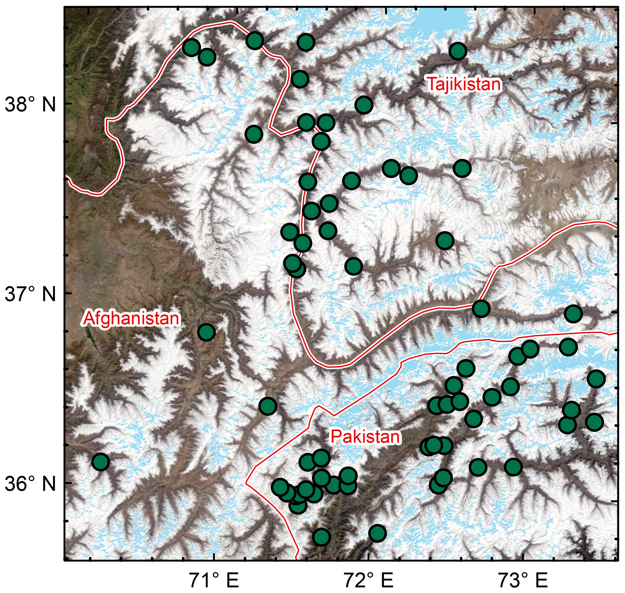
Figure 1Study region with AKAH stations (green dots) overlaid on a MODIS true-color image from 13 April 2018. Also shown are the country boundaries (red) and glacierized areas (light blue) from the Global Land Ice Measurements from Space dataset (Raup et al., 2007). All of the stations in Afghanistan and Tajikistan are in areas that eventually flow into the Amu Darya. All of the stations in Pakistan are in areas that eventually flow into the Indus River. Imagery courtesy of NASA Worldview.
Although there have been a large number of studies examining the glaciers of High Mountain Asia, there are fewer studies examining snowfall in High Mountain Asia, which is odd, since hydrologically in this region, snow on land melt provides the vast majority of runoff compared to snow on ice and melting glacier ice (Armstrong et al., 2018). Many of these studies are focused on the region to the east of the AKAH study area, shown in Fig. 1. To our knowledge, there have been no studies on snowpack stratigraphy in the AKAH study area, and we were unable to obtain any snow pit measurements from this area.
A few studies have specifically examined snowfall in larger regions that include some of the AKAH stations, mostly for stations in the southern basins that flow into the Indus River – that is, all of the stations in Pakistan. The rest of the stations in Afghanistan and Tajikistan are in basins that flow into the Amu Darya. The most comparable study (Shakoor and Ejaz, 2019) examines the Passu catchment in the Hunza River basin, on the right in Fig. 1. As in this study (Sect. 5.1), Shakoor and Ejaz (2019) also use the SNOWPACK and Alpine3D models. Model parameters were calibrated using a single weather station, Urdukas, at 3926 m elevation near the Baltoro Glacier (Ev-K2-CNR, 2014), with 1 year of precipitation measurements, using snow depth for validation. The authors report overestimation of the measured snow depth at the calibration station, even after questionable adjustments to the snow albedo and other model parameters. For example, the snow and ice albedo is given as 0.20 to 0.30 (Table 3, Shakoor and Ejaz, 2019), which would make it 0.10 to 0.20 lower than some of the lowest measured broadband albedo values for dirty snow (Bair et al., 2019b; Skiles and Painter, 2016). They attribute the overestimation to problems with the precipitation measurements, common for high-elevation stations. One problem with the Urdukas station in particular is that the tipping-bucket precipitation gauge is unheated, making it unusable for measuring solid precipitation. Temperatures at this station were well below freezing for the winter and most of the spring, which explains why no precipitation was recorded from January until sometime in March during 2012, the calibration year.
Viste and Sorteberg (2015) study several gridded precipitation products throughout High Mountain Asia, including the Indus Basin. They report that while total precipitation was similar across the products – including MERRA (Rienecker et al., 2011), APHRODITE (Yatagai et al., 2012), TRMM (Huffman et al., 2007), and CRU (Harris et al., 2014) – the total snowfall varied by a factor of 2 to 4. Smith and Bookhagen (2018) used 24 years (1987 to 2009) of satellite-based passive microwave SWE estimates to examine trends throughout High Mountain Asia, including the Amu Darya and Indus basins. Their SWE estimates show most 25 km pixels in this region in the 50–100 mm range for December through February, with a few over 100 mm in the Amu Darya basin (i.e., all the AKAH stations in Afghanistan and Tajikistan) and none over 100 mm in the Indus Basin (i.e., all the AKAH stations in Pakistan), likely too low by an order of magnitude for some pixels given our previous reconstructed SWE values and limited climate measurements in Afghanistan (Bair et al., 2018a).
For the AKAH stations in Tajikistan, the most comprehensive snow measurements come from Soviet snow surveys (mostly depth, but with some SWE and density measurements) that have been digitized (Bedford and Tsarev, 2001). Most of these measurements begin in the late 1950s and end around the fall of the Soviet Union, in either 1990 or 1992, making them useful for climatological studies but not for validation of modern satellite-based estimates.
The sole source of accessible snow measurements in Afghanistan was a table of outdated World Meteorological Organization (WMO) monthly climatological data from Kabul (elevation 1791 m) and North Salang (elevation 3366 m), showing the maximum monthly snow depth and the mean number of days with snow (Table 1 in Bair et al., 2018a). Again, these measurements are not useful for validating more modern snow estimates.
There have been many other studies that have attempted to estimate basin-wide precipitation (including snowfall) for larger areas that include the AKAH region, especially in the Indus. Several climate studies of the Indus have focused on using lower-elevation precipitation gauges, which are then used to spatially interpolate basin-wide precipitation. Dahri et al. (2016) and Dahri et al. (2018) have assembled perhaps the largest collection of climatological measurements covering the AKAH region, mostly based on gauge measurements, as part of a study on the hydrometeorology of the Indus Basin. Using undercatch corrections based on wind, often from reanalysis, they increased precipitation estimates by 21 % on average throughout the Indus Basin (Dahri et al., 2018). For example, in the Gilgit sub-basin, they find an unadjusted precipitation estimate of 582 mm yr−1, adjusted to 787 mm yr−1, a 35 % increase. Although some of the measurements are taken from publicly available sources, as with most publications for this region, the comprehensive data used are not publicly accessible.
A similar but less sophisticated approach was used by Lutz et al. (2014), who used a constant increase of 17 % across the APHRODITE precipitation dataset, which covers all of High Mountain Asia. Immerzeel et al. (2015) used glacier mass balance estimates with streamflow measurements as validation to show that high-altitude precipitation in the upper Indus Basin is 2 to 10 times what is shown using gridded precipitation products like APHRODITE. Bookhagen and Burbank (2010) estimate that snowmelt contributes 66 % of annual discharge to the Indus and averages 424 mm across the basin.
In summary, quite a few studies have produced varying precipitation and snowfall estimates for the AKAH region, with no recent in situ snow measurements from Afghanistan or Tajikistan.
Our previous work (Bair et al., 2018a) used a simple density model (Sturm et al., 2010) based on snow climatology (Sturm et al., 1995) and day of year to model SWE from the manual snow depth measurements. The density model itself has −12 % to 26 % bias in predicting SWE. When taking into account geolocational uncertainty of the reconstructed SWE estimates and uncertainty in the density model, errors are on the order of 11 %–13 % mean absolute error (MAE) and −2 % to 4 % bias, depending on the date. However, we only examined 1 year of the AKAH station data (2017), and the high uncertainty in the density model itself begs a more sophisticated approach.
From recent work (Bair et al., 2018b), we have shown that the SNOWPACK (Lehning et al., 2002a, b; Bartelt and Lehning, 2002) model is capable of accurate SWE prediction when supplied only with snow depth for precipitation as well as the other requisite forcings (i.e., radiation, snow albedo, temperatures, and wind speed). Over a 5-year period using hourly in situ measured energy balance forcings and a snow pillow for validation at a high-elevation site in the western US, the SWE modeled by the numerical snow cover model SNOWPACK showed a bias of −17 mm, or 1 % (Bair et al., 2018b). Likewise, the success of the Airborne Snow Observatory (Painter et al., 2016) has demonstrated that given accurate snow depth measurements, SWE can be well modeled.
Our modeling approach consisted of (a) downscaling forcings in the Parallel Energy Balance Model (ParBal) and reconstructing SWE, (b) combining the downscaled forcings for each AKAH station with temporally interpolated manual snow measurements, (c) running SNOWPACK for each of the AKAH stations with the downscaled and interpolated measurements from (a) and (b), and (d) running Alpine3D using the output from SNOWPACK, notably the hourly precipitation. In addition to predicting SWE, the SNOWPACK–Alpine3D coupled model also predicts stratigraphic parameters useful for avalanche forecasting, thereby giving us an idea of the layering and stability in this region. For comparison, we also ran the Noah-Multiparameterization (Noah-MP) land surface model over the region with widely used forcings. We also compared spatial estimates of SWE from GLDAS-2. Methods are summarized in Table 1 and explained below, with more detail provided in Appendix A.
5.1 SNOWPACK and Alpine3D
SNOWPACK and Alpine3D are freely available (https://models.slf.ch, last access: 15 May 2019) point and spatially distributed snow models, courtesy of the Swiss Snow and Avalanche Research Institute SLF. SNOWPACK is the older of the two and uses finite elements to model all of the layers in snowpack at a point.
Table 1Summary of models used. See Sect. 5 and Appendix A for an explanation of acronyms and further details.

SNOWPACK has shown promising results in both operational (e.g., Lehning et al., 1999; Nishimura et al., 2005) and research applications (e.g., Bellaire et al., 2011; Hirashima et al., 2010). Previous results with SNOWPACK (Bair et al., 2018b) show high model sensitivity to precipitation but only a 1 % error in modeled SWE when using snow depth only (not total precipitation) as a forcing. Thus, given reliable snow depth measurements at each AKAH station (see Sect. 5.5), modeled SWE during the accumulation season is treated as having negligible uncertainty. During the ablation season (after peak SWE), uncertainty is higher. Unlike during snow accumulation events, SNOWPACK does not force its modeled snow ablation to match the measured snow depth decreases. Uncertainty in SWE during the ablation season is then largely dependent on radiative forcings (Marks and Dozier, 1992) and the broadband snow albedo (Bair et al., 2019b). Here, 5 % uncertainty is used, based on the MAE from SWE reconstructions using the same remotely sensed forcings at a continental subalpine site (Bair et al., 2019b). In the same study, a small (3 %) bias in SWE was also found, but this is likely due to shortcomings with the reconstruction method and not applicable to SWE modeled with SNOWPACK. Thus, the small bias was ignored. We acknowledge that these uncertainty estimates are themselves uncertain; e.g., the reanalysis forcings could be especially poor for this region compared to those available in the western US.
Alpine3D (Lehning et al., 2006) is essentially a spatially distributed version of SNOWPACK with a number of additional modules, including terrain-based radiation modeling, blowing snow, and hydrologic modeling. Integral to Alpine3D is SNOWPACK, which is run for each pixel, as well as the MeteoIO library (Bavay and Egger, 2014), which provides a large number of temporal and spatial interpolation functions that can be used on forcings for Alpine3D and SNOWPACK.
5.2 The Parallel Energy Balance Model
ParBal was created at UC Santa Barbara and designed for reconstruction of SWE. It is also publicly available (https://github.com/edwardbair/ParBal/releases/tag/v1.0). Currently, ParBal is designed to use downscaled temperature, pressure, and humidity from version 2 of the Global or National Land Data Assimilation System (GLDAS-2 and NLDAS-2; Xia et al., 2012; Rodell et al., 2004), shortwave and longwave radiation from Edition 4A of the Clouds and the Earth's Radiant Energy System (CERES; Rutan et al., 2015) SYN product, and time–space-smoothed (Dozier et al., 2008; Rittger et al., 2020) snow surface properties from MODIS Snow Covered Area and Grain Size (MODSCAG; Painter et al., 2009) and MODIS Dust and Radiative Forcing in Snow (MODDRFS; Painter et al., 2012). ParBal is run hourly at 500 m spatial resolution, and forcings are adjusted for terrain and elevation. The main output is the residual energy balance term, which is assumed to go into melt when positive during the ablation phase after cold content is overcome (Jepsen et al., 2012). This residual melt term is then summed in reverse during periods of contiguous snow cover and multiplied by the fSCA to spread the snow spatially. The errors in SWE from ParBal are mostly from fSCA and the radiative forcings. Errors and details on ParBal are covered extensively in Bair et al. (2016) and Rittger et al. (2016). In the supplement for Bair et al. (2018a), the errors arising from using GLDAS-2 and CERES 4A (available worldwide but at coarser spatial resolution) vs. NLDAS-2 are specifically evaluated. Using 3 years of basin-wide SWE estimated by the Airborne Snow Observatory in the upper Tuolumne basin, California, USA, the MAE for ParBal was 25 mm, or 26 % (Bair et al., 2018a).
5.3 Global Data Assimilation System 2 (GLDAS-2)
For comparison, we also include the SWE estimates from GLDAS-2 (Noah). SWE from GLDAS-2 has been shown to be comparable to estimates from other reanalysis datasets but negatively biased by about 60 % in comparison to higher spatial datasets with assimilation from snow station measurements (Broxton et al., 2016).
5.4 Noah-Multiparameterization (MP)
The Noah-MP v3.6 (Niu et al., 2011; Ek et al., 2003) land surface model, forced using MERRA-2 (Gelaro et al., 2017), was used to simulate the hydrologic cycle over the study area and provide SWE estimates for comparison with ParBal and the Alpine3D output. Noah-MP was selected due to its detailed representation of the snowpack relative to other land surface models. The model subdivides the snowpack into up to three layers with associated liquid water storage and melt and refreeze capability (Yang and Niu, 2003; Niu and Yang, 2004). It incorporates the exchange of heat and moisture through the snowpack between the land surface and the atmosphere. In a model intercomparison study using a 2 km spatial resolution regional climate model for forcings, Chen et al. (2014) show that Noah-MP modeled peak SWE at SNOTEL sites in Colorado, USA, with a −7 % bias.
5.5 Use of AKAH station measurements
We modeled daily SWE at the AKAH stations during the 2017 and 2018 water years (WYs) primarily using the manually measured height of snow (HS), also called snow depth, combined with our downscaled energy balance parameters (for downscaling methodology, see Rittger et al., 2016; Bair et al., 2016, 2018a). To our knowledge, no quality control was performed on the AKAH station measurements before we received them. We choose the manual HS and new (24 h) snow (HN) as the only variables to use from the AKAH stations. The HS appeared to be the most reliably measured, as that only requires reading a value from a master snow depth stake. Apart from spurious drops or missing values (see below), the HS measurement appeared consistent and believable at most of the stations, implying an accurate snow depth record. The HN was used to correct a data entry problem in 2017 that we discuss below. The reliability of the other measurements (instantaneous wind speed and direction, maximum and minimum temperature, and rainfall) was questionable. For example, we were not provided with sensor or measurement metadata, e.g., sensor make and model, measurement height, and whether or not the temperature sensor was shielded from shortwave radiation. These other measurements taken daily were also of limited value for interpolation to hourly values (see item 3 below). Thus, these other measurements were not used.
The AKAH dataset had a number of shortcomings that we list here along with how we addressed them.
-
Some of the stations recorded no snow at all, especially in the dry 2018 year, or had obvious problems, such as weeks of missing measurements, so they were excluded. For 2017, 52 (54 %) of stations were used. For 2018, 41 (46 %) stations were used.
-
There were spurious drops in the HS measurements. The drops were clearly cases of missing values being filled with zeros. These measurements were manually flagged and converted to null values for interpolation (see below).
-
The daily measurements had to be interpolated to hourly values. For the most part we used linear interpolation, although this is not ideal during snow accumulation, since it is almost never the case that snowfall is uniform over a 24 h period. This is a problem that affects the accuracy of snow settlement estimated by SNOWPACK. There were two cases where other interpolation methods were used. If there were several days of missing values, we used a nearest-neighbor interpolation to fill in the missing daily values, followed by a linear interpolation from daily to hourly measurements such that we assumed that all the new snow fell in a 24 h period. The other case was for days where the linear interpolation would yield a value below the minimum threshold hard-coded into SNOWPACK (0.5 cm h−1) for the first accumulating snowfall on bare ground. In this case, a previous neighbor interpolation was used in such a way that the entire snowfall occurred in the last hr prior to the next day's measurement.
-
We found the AKAH stations suitable for snow on the ground measurements but not for rainfall or total (solid plus liquid) precipitation. This was only an issue for the Alpine3D snow modeling, as snow measurements were being extrapolated to higher elevations than the AKAH stations (Sect. 6.2); thus at these higher elevations, snow accumulated earlier and melted later than at the lower AKAH stations.
Given the near-total lack of canopy cover in the region, we suspected substantial undercatch from rain gauges. Using the wind speed, an undercatch correction would have been possible given more information on the gauges (e.g., orifice opening diameter and whether or not a shield was present); however these instrument metadata were not available to us. Likewise, we did not know if the gauges were heated or not.
Further, the time period for recording measurements from the stations was not consistent. In WY 2017, measurements began being reported on 10 November 2016 and were reported until 24 November 2017. However, in WY 2018, measurements were not reported until 1 December 2017, and no station measurements were reported past 1 April 2017. The reporting period likely covered all the snowfall events but not all the precipitation events.
To address the rainfall measurement and reporting issues, we used GLDAS Noah v2.1 (Rodell et al., 2004) rainfall and snowfall from the nearest grid cell ( spatial by 3 h temporal resolution) to fill in precipitation prior to the first measurements in each water year and after 1 April for both water years. We did not account for rain from 10 November 2016 to 1 April 2017 and from 1 December 2017 to 1 April 2018; instead we relied on the modeled precipitation from SNOWPACK using snow depth. The AKAH station observations show that rain during this time period was rare.
- 5.
A database problem prevented snow heights >100 cm from being entered into the database for a few days in 2017. This problem became apparent during February 2017, when the Nuristan avalanches took place (United Nations, 2017), as that is the first time that most stations recorded values >100 cm. Values were shown as 100 cm on multiple days, followed by values >100 cm. To address this issue, we flagged all the values equal to 100 cm prior to peak snow depth in 2017 and then marked those as null values. We then filled those null values using the cumulative sum of new snow during that time.
5.6 Analysis of modeled snow profiles
For holistic measures of the snow profiles modeled in Alpine3D, we used two metrics from Bellaire et al. (2018): (1) the fraction of facets and (2) the number of critical layers. The fraction of facets is the height of all the layers containing faceted crystals, i.e., International Classification for Seasonal Snow on the Ground primary codes FC, DH, and SH (Fierz et al., 2009), divided by the height of the snowpack. The number of critical layers was computed using a threshold sum approach (Schweizer and Jamieson, 2007) with modifications for simulated profiles (Monti et al., 2014, Table 1). In each profile, six different variables (grain size, difference in grain size, hardness, difference in hardness, grain type, and depth) in the top meter of the snowpack (from the surface) were checked against threshold values. Layers exceeding five or more thresholds were classified as critical.
The fraction-of-facets metric does not have a validation study, but faceted layers are a weak crystal form and are responsible for 43 % (Bair et al., 2012) to 67 % (Schweizer and Jamieson, 2001) of investigated avalanches. Layers classified as critical using the threshold sum approach above corresponded to failure layers about half of the time to failure layers found with compression tests (Monti et al., 2014), an in situ snowpack stability test (van Herwijnen and Jamieson, 2007; Jamieson, 1999).
5.7 Spatial scale for comparisons
Because ParBal is the only model run at 500 m spatial resolution and all the other models were run at ∼25 km, it is the only model appropriate for point comparisons, although point-to-area problems are still an issue. To address the geolocational uncertainty for the gridded MODIS products, which can be up to one ∼500 m pixel (Tan et al., 2006; Xiaoxiong et al., 2005) and spatial variability of the snow, we used a 9-pixel neighborhood centered on each AKAH station and chose the best fit to the SNOWPACK-modeled SWE. This approach has been used in previous work (Bair et al., 2018a; Rittger et al., 2016). We also include the high and low SWE values in that surrounding 9-pixel neighborhood to bound the uncertainty.
For all of the other model comparisons, we resampled all of the model output to a UTM (Zone 43S) grid with 25 km pixels, close to the native resolution of the Noah-MP and GLDAS2 grid used (0.25∘). This yielded a study area of 105 625 km2 (13 pixels ×13 pixels, each 25 km2 in area). The ParBal output had to be significantly upscaled from 500 m to 25 km using Gaussian pyramid reduction (Burt and Adelson, 1983) in steps, with bilinear interpolation for the final step.
The relationships between the components are summarized in Fig. 2. The results discussed below are comparisons of (1) SWE and (2) snow stratigraphy across (a) all of the AKAH stations (points) and (b) the entire study region.

Figure 2Summary of relationships between the various components. Forcings are shown in red, models and selected outputs are shown in blue, and the comparisons discussed below are shown in green. The black arrows show the direction of inputs.
6.1 Point comparisons between SNOWPACK and reconstructed SWE
A first step for any SWE reconstruction comparison is to determine when the ablation season starts. This varies for different years and at different sites (e.g., Margulis et al., 2016). Using the SNOWPACK-modeled SWE, we can examine the peak SWE dates for both years for all of the AKAH stations (Fig. 3a, b). Peak SWE dates vary across the stations and years, but the median values between years are a week apart, 19 February 2017 and 26 February 2018. Thus, we use those dates for our comparisons.
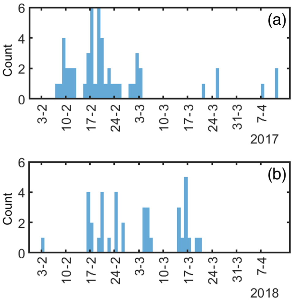
Figure 3Peak SWE dates, modeled by SNOWPACK for 2017 (a) and 2018 (b) for each of the AKAH stations. The median peak SWE dates are 19 February 2017 and 26 February 2018. N=52 and 41 AKAH stations used for 2017 and 2018.
To create a holistic comparison for all the stations across the ablation period, mean SWE values were computed and plotted for each day during the ablation season (Fig. 4). For the reconstructed SWE on 19 February 2017, the bias is −77 mm (−28 %). For the reconstructed SWE on 26 February 2018, the bias is −6 mm (−9 %). Thus, together these biases average to −42 mm (−19 %). The high–low values in the 9-pixel neighborhood show the wide spatial variation in SWE estimates and are to be expected in these deep valley sites (Sect. 6.2). The increases in reconstructed SWE during the ablation season are caused by differences in how melt is summed for any given pixel. In ParBal, melt is only summed during periods of contiguous snow cover. This means that if a pixel containing an AKAH station has no snow on it at some point during the ablation season, but then snow is detected, it causes an increase in the mean SWE. This is called an ephemeral snow event, i.e., snow that disappears and reappears. For a more in-depth examination of the error at individual stations, a box plot is shown for the median peak SWE dates for both years (Fig. 5). The median bias of the reconstructed SWE is −11 mm (−14 %).
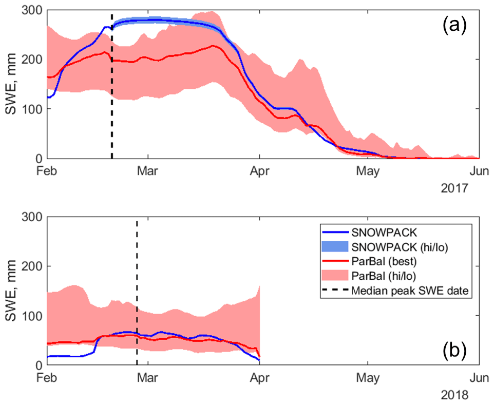
Figure 4Mean SWE for 2017 (a) and 2018 (b) modeled at all of the AKAH stations using SNOWPACK (blue lines) compared to reconstructed SWE from ParBal using a best-of-9-pixel approach (red lines). Also plotted is the median peak SWE date. The high–low (hi/lo) bounds (filled areas) represent uncertainty. For ParBal, uncertainty is expressed as the range of values in the 9-pixel neighborhood. For SNOWPACK, uncertainty is 5 % of the modeled SWE during the ablation season. See Sect. 5.1 and 5.2 for details. The modeled SWE values end abruptly on 1 April 2018 because the AKAH stations stopped reporting due to drought conditions. The number of stations used is the same as in Fig. 3.
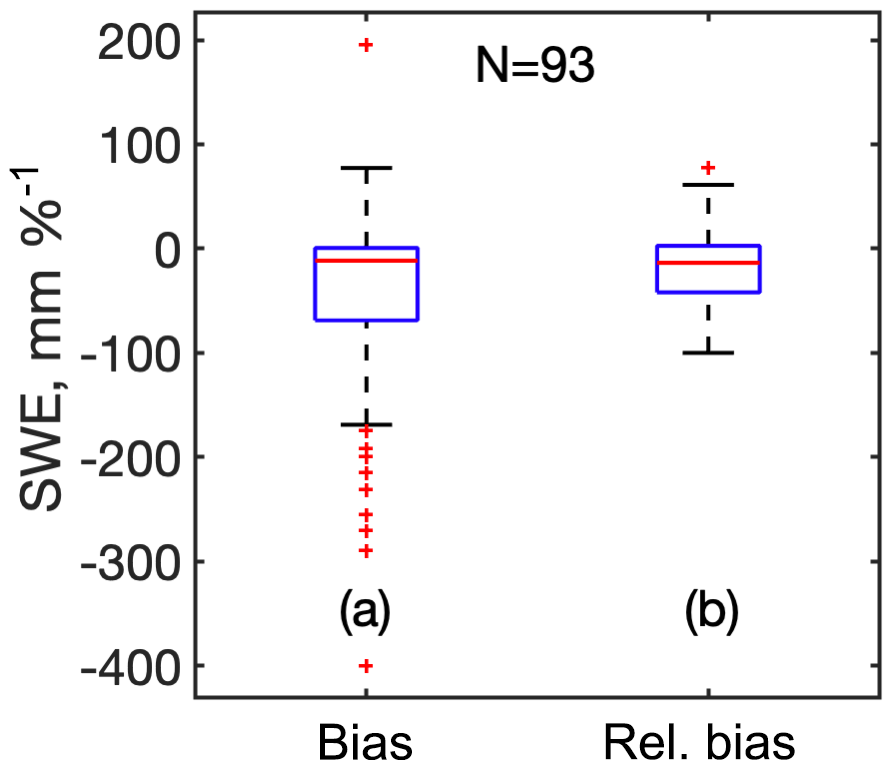
Figure 5Bias (a) and relative bias (b) for ParBal reconstructed SWE vs. Alpine3D-modeled SWE at AKAH stations on the median peak SWE date for both years, where bias here is ParBal SWE and Alpine3D SWE.
6.2 Four model spatial comparisons
The AKAH stations are lower than the average elevation for the region. The average elevation of the AKAH stations is 2619 m (1735 to 3410 m). But when the 500 m DEM (digital elevation model) is upscaled to 25 km, the average elevation of the pixels containing the AKAH station is 3858 m, with a range of 2517 to 4764 m. This has two important implications: (1) much of the higher elevation snowfall is being extrapolated and (2) the higher elevation causes the peak SWE date to move forward in time. The median peak SWE dates for the (N=169) 25 km pixels encompassing the study area are 5 May 2018 and 3 May 2018. Thus, we use the median of the two to compare our reconstructed SWE values (Fig. 6a, b; Fig. 7a–d; and video in the Supplement).
The range between models is striking. Noah-MP has the highest peaks (562 mm in 2017 and 331 mm in 2018) but is among the first to melt out. The reconstructed SWE from ParBal only shows minor variation between the 2017 peak (240 mm) and the 2018 peak (206 mm). ParBal and GLDAS-2 melt snow out latest in both years. This is especially true for ParBal in 2017, where the Supplement video shows that ParBal has snow cover over more pixels that persists for longer into the melt season but is lower in SWE than the other models. The Alpine3D model shows the second highest peak SWE in 2017 (469 mm) but the lowest peak (165 mm) in 2018. The comparatively higher values from Noah-MP could result from relatively high precipitation estimates from its MERRA2 precipitation forcings. Similarly, Viste and Sorteberg (2015) report that MERRA (version 1) showed higher snowfall in the Indus Basin than any other reanalysis or observation-based forcing dataset.
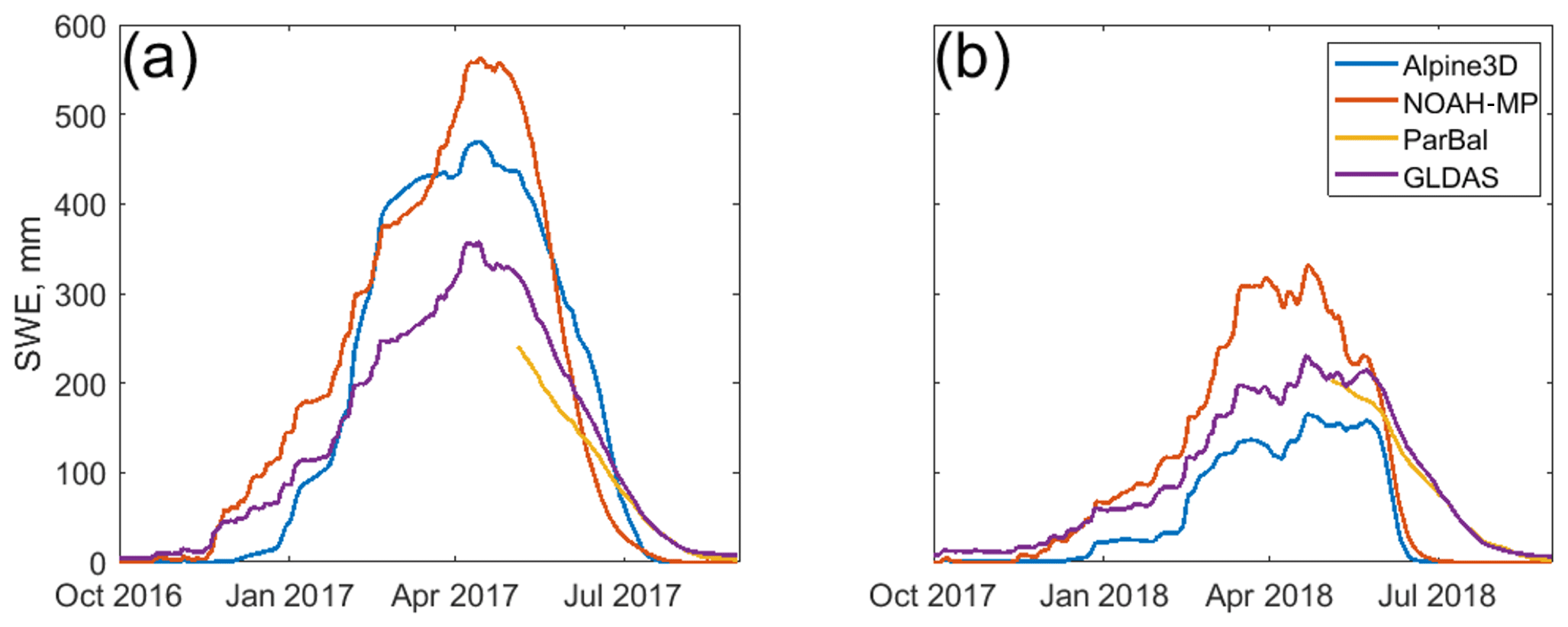
Figure 6Time series of mean SWE for four snow models across the study area (13 pixels ×13 pixels, each 25 km2) shown in Fig. 1 for 2017 (a) and 2018 (b). The reconstructed SWE from ParBal (yellow) goes back to 4 May, the median peak SWE date for both years, since reconstruction is only valid during the ablation season.
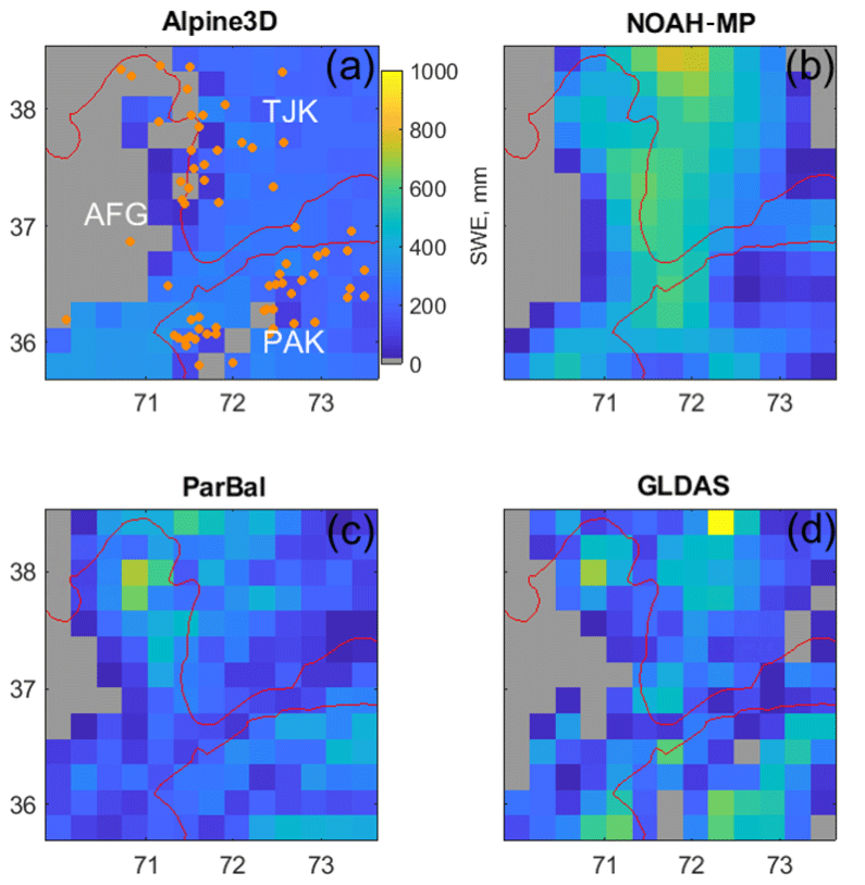
Figure 7Four-model (a–d) spatial comparison for the study area on 4 May 2018. The white letters represent the following: AFG – Afghanistan; TJK – Tajikistan; and PAK – Pakistan. Also shown in (a) are the locations of the AKAH stations (orange points). This is a frame from a video sequence available in the Supplement.
Since Alpine3D relies heavily on extrapolation of SWE, we suggest that its mean SWE values plotted in Fig. 6 could have higher uncertainty than some of the other models. For example, the Alpine3D pixels seem to melt out early compared to the other models, especially ParBal, which is the only model that relies on satellite-based estimates of fSCA (see Supplement video). Thus, Alpine3D may computing too little SWE in cold, high-elevation areas that melt slowly. These problems are all indicative of stations that are located in valley bottoms and that only cover the lowest elevations across these 25 km pixels.
The ParBal results are confounding given that the agreement between the modeled SWE from ParBal and SNOWPACK at individual AKAH stations (Fig. 4a, b) is much better for both 2017 and 2018.
For insight into potential biases in the modeled spatial SWE from ParBal, we carefully studied the snow-covered area (SCA; not just for 2017 and 2018 but since 2001), the potential melt (i.e., the melt if a pixel were 100 % snow covered), and the melt from glacierized areas (light blue in Fig. 1). We did not find any errors in the model, its parameters, or its forcings. Thus, it is possible that the ParBal SWE is biased low in 2017 for reasons that we could not discern or that the other models are biased high. To note is that the 2017 and 2018 SCA (Fig. 8; purple and orange) is very similar for both years during the ablation period, especially at the end of the ablation season.
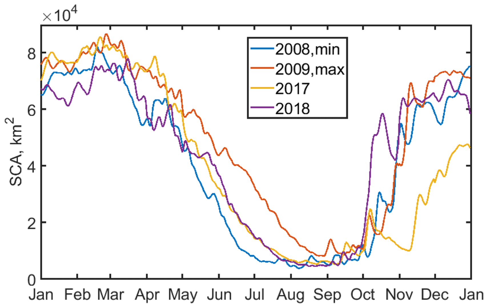
Figure 8Time series of snow covered area from spatially and temporally interpolated MODSCAG (Rittger et al., 2020), an input for ParBal, for 4 selected years across the region. Years 2008 and 2009 had the lowest and highest values on 1 July over the period of record from 2001 to 2018, while 2017 and 2018 comprise the AKAH station study period.
Since pixels do not contribute uniformly to melt, SCA alone cannot be used to predict SWE, but in general years with less snow they have lower SCA values towards the end of the ablation season. Figure 8 shows that 2017 and 2018 were similar in terms of SCA from April to melt out. Thus, the large difference between 2017 and 2018 for the AKAH station SWE, but small differences in SCA and spatially averaged reconstructed SWE suggest that 2017 may have been a larger snow year at the lower elevations where the AKAH stations are but similar to 2018 at the higher elevations.
6.3 Stratigraphy and stability
The simulated snow profiles from the AKAH stations (Fig. 9a, b) and the 25 km pixels containing the AKAH stations (Fig. 10a, b) show very different snowpacks. Because of the induced increase in elevation from scaling (e.g., from an average of 2619 to 3858 m; Sect. 6.2), the 25 km pixels show a deeper but more faceted snowpack with critical layers that persist for a month or longer. In 2017, for the median AKAH station values, the snowpack reaches a maximum of 76 % facets on 21 January (Fig. 9a). In 2018, the snowpack reaches a maximum of 71 % facets (Fig. 9b). There were no critical layers simulated. In contrast, for the median values in the 25 km pixels for both years, the height of snow (HS) is approximately 2 times that for the stations (Fig. 10a, b). The snowpack reaches a maximum of 94 % facets in 2017, with one critical layer persisting for 35 d (Fig. 10a). The snowpack in 2018 reaches 95 % facets, with one or two critical layers persisting for 80 d (Fig. 10b). During the Nuristan avalanches on 4 to 7 February 2017 that killed over 100 people (United Nations, 2017), the AKAH stations show the largest 3 d snowfall of the study period (Fig. 9a), and the results for the 25 km pixels show large snowfall occurring on top of the only critical layer of the season (Fig. 9b). That is a classic avalanche scenario, i.e., a large snowfall on a weak snowpack.
In lieu of any type of snow profile from this region, these profiles paint the best picture of the snow conditions available. A relatively stable snowpack seems to be present in the valleys, where the AKAH stations are located. But at the higher elevations, the simulated profiles show a more critical snowpack. This is especially serious, considering that these villages are in the run-out zones of these potentially unstable snowpacks. In some cases, several thousand meters of vertical relief loom above the villages. For example, Yarkhun Lasht (36.795∘ N 73.022∘ E; elevation of 3249 m) in Pakistan is flanked by 6500 m peaks on both sides of its valley.
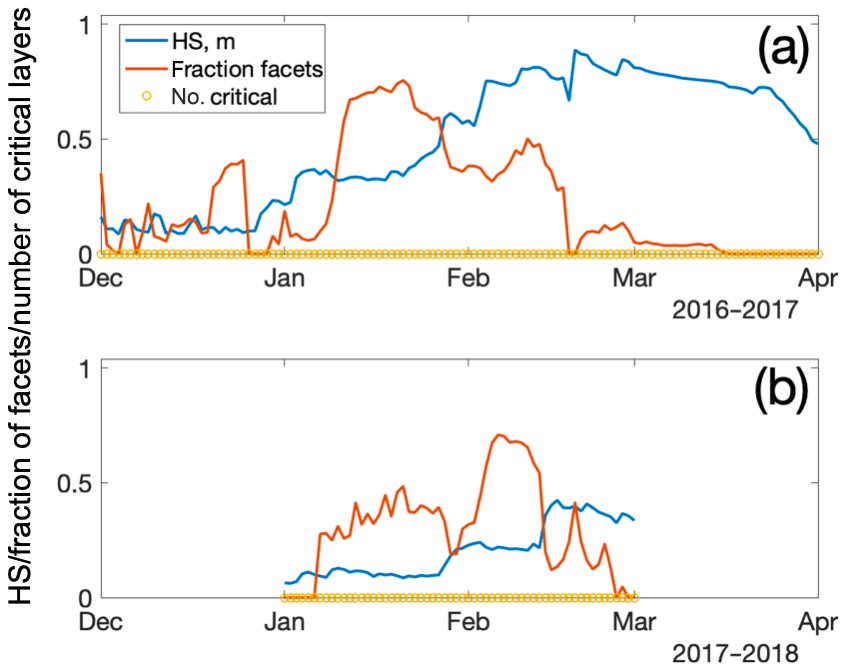
Figure 9Stratigraphy summary of the AKAH stations for 2017 (a) and 2018 (b). Plotted are the median values of the following: height of snow (HS), fraction of the snowpack containing facets, and number of critical layers. The number of stations used to compute the medians varied due to snow coverage.
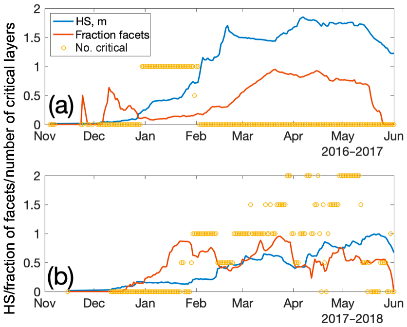
Figure 10Stratigraphy summary of the (13×13) 25 km pixels containing AKAH stations for 2017 (a) and 2018 (b). Plotted are the median values of the following: height of snow (HS), fraction of the snowpack containing facets, and number of critical layers.
Knowledge of the snowpack in northwestern High Mountain Asia is poor. This area is subject to droughts and threatened by snow avalanches. Both problems can be aided by improved knowledge of the snowpack. Thanks to a novel operational avalanche observation network, there are now daily snow measurements at a number of operational weather stations in this austere region. In this study, 2 years of daily snow depth measurements from these stations were combined with downscaled reanalysis and remotely sensed measurements to force a point and spatially distributed snow model. Compared to a previous effort (Bair et al., 2018a), this study represents a substantial improvement in SWE modeling for the region and a first attempt to characterize region-wide snow stratigraphy. At the point scale, SWE estimates from a reconstruction technique that does not use precipitation or in situ measurements compared favorably. At the regional scale, four models showed a wide spread in both peak SWE and melt timing. For the models that rely on in situ precipitation measurements, a major challenge is spatial extrapolation, as many of the stations are located in deep valleys. Adding measurements from the mountains above would facilitate more realistic lapse rates, but these measurements do not currently exist, although they would be beneficial both for operational avalanche safety and for scientific studies.
In the regional comparison, SWE estimates from ParBal were on the low end, but given the model spread it is difficult to form a consensus estimate. We plan additional in situ validation at other sites in High Mountain Asia to continue to assess the performance of ParBal there.
The simulated profiles showed very different snowpacks. At the point scale at lower elevations in the valleys, profiles showed fewer facets and almost no critical layers, while at the regional scale for higher elevations, the profiles showed heavily faceted snowpacks with critical layers that persisted throughout the winter and spring.
A1 ParBal
ParBal was configured and forced as described in Bair et al. (2018a) and Bair et al. (2016). The model time step was 1 h. The DEM used was the ASTER GDEM version 2 at 1 arcsec (NASA JPL, 2011), while the canopy type and fraction were taken from the Global Land Survey at 30 m (USGS, 2009). The shortwave and longwave forcings were downscaled from the CERES SYN Edition 4A 1∘ by 1 h product (Rutan et al., 2015), while the air temperature, specific humidity, air pressure, and wind speeds were downscaled from the GLDAS Noah version 2.1 0.25∘ by 3 h product (Cosgrove et al., 2003). Time–space-smoothed (Dozier et al., 2008; Rittger et al., 2020) fSCA and grain size from MODSCAG (Painter et al., 2009) was combined with the visible albedo degradation from dust in MODDRFS (Painter et al., 2012) to produce snow hourly snow albedo.
A2 Noah-MP
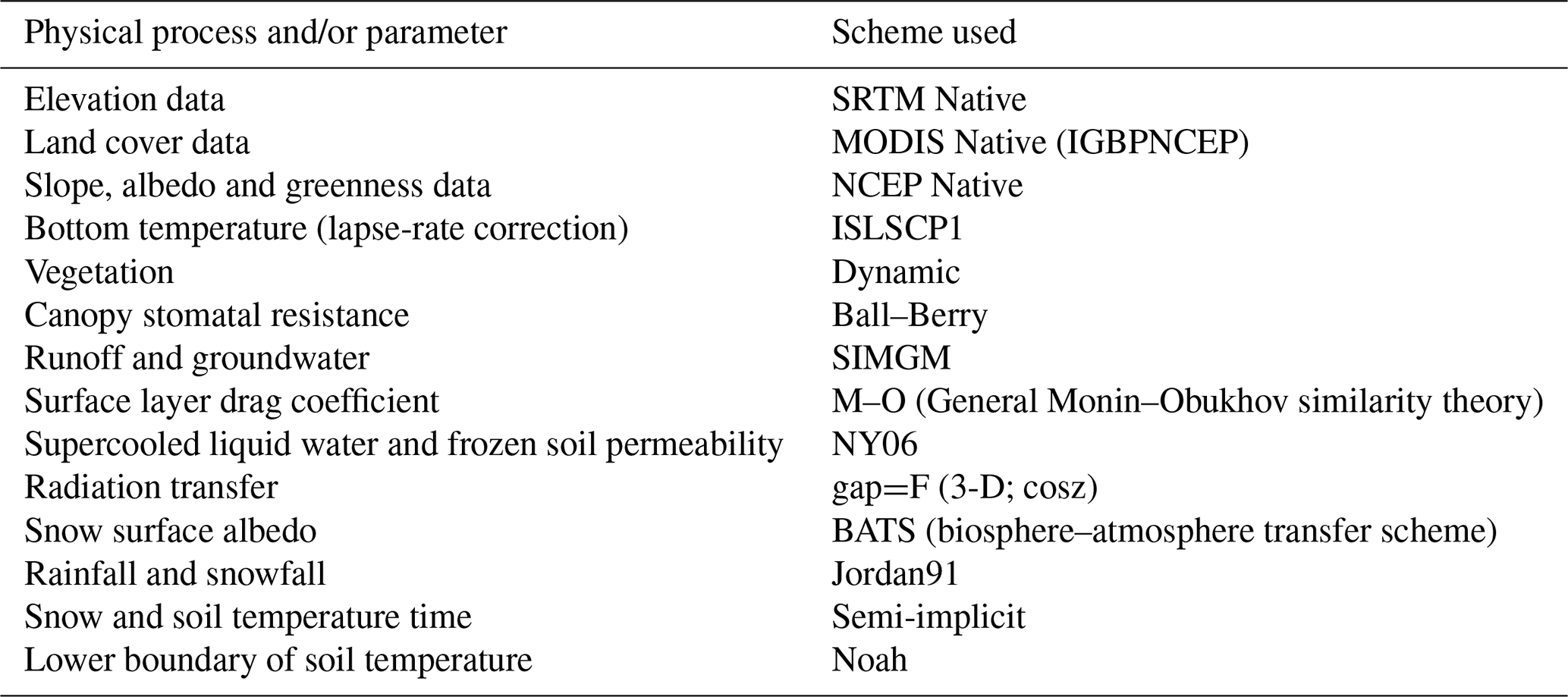
Noah-MP v3.6 was run in retrospective mode within the NASA Land Information System (LIS) framework. A state vector ensemble (total 30 replicates) was generated by perturbing the forcings to account for the state uncertainty during forward propagation of the model. MERRA-2 (Gelaro et al., 2017) forcings were utilized with bilinear spatial and linear temporal interpolation. The model was run on an equidistant cylindrical grid with 0.25∘ spatial resolution and a 15 min model time step. The spin-up time extended from May 2002 to May 2016, while the study period was from June 2016 to October 2018. The number of maximum layers in the snowpack was three. Table A1 provides details of the Noah-MP scheme options selected. Further details regarding each scheme and relevant references can be found at https://ral.ucar.edu/solutions/products/noah-multiparameterization-land-surface-model-noah-mp-lsm (last access: 15 May 2019).
Table A1Noah-MP v3.6 physical parametrization scheme options utilized in this study.
A3 SNOWPACK
SNOWPACK v3.50 was run in research mode at a 15 min time step, with hourly outputs for each of the AKAH stations. Hourly forcings were computed by combining temporally interpolated snow depth from the AKAH manual measurements with air temperature, incoming shortwave, reflected shortwave, incoming longwave, wind speed, and relative humidity from the downscaled ParBal outputs, as described in Sect. 5.2. SNOWPACK was only run for periods when measurements from the AKAH stations were available in November–December to April–May, depending on the year.
Plots were assumed to be level, so forcings without terrain correction were applied, except for shading, when the sun was below the local horizon, e.g., a mountain was blocking the sun (Dozier and Frew, 1990). The wind direction, which is not available in GLDAS-2, was fixed at the mean value from the daily AKAH instantaneous values. The ground temperature was set as the minimum of the air temperature or −1.5 ∘C when snow cover was present.
Aside from setting required parameters and values for inputs and outputs, changes to default parameters that affected model output are provided in Table A2.

A4 Alpine3D
Alpine3D version 3.10 was run using with the outputs produced by SNOWPACK as forcings for each of the AKAH stations at 25 km resolution. The DEM and land cover (incorrectly labeled land use in the Alpine3D documentation) data were upscaled from the ParBal data. Alpine3D was run at an hourly time step using hourly forcings, with daily outputs using the “enable-eb” switch. Other switches were set to off, the defaults. The “enable-eb” switch computes the terrain radiation with shading and terrain reflections (see Alpine3D documentation at https://models.slf.ch (last access: 15 May 20019) for a description).
To extend the length of the model runs, for each AKAH station, GLDAS-2 precipitation was appended to periods prior to the first AKAH observation for the year and after the last, as described in Sect. 5.5.
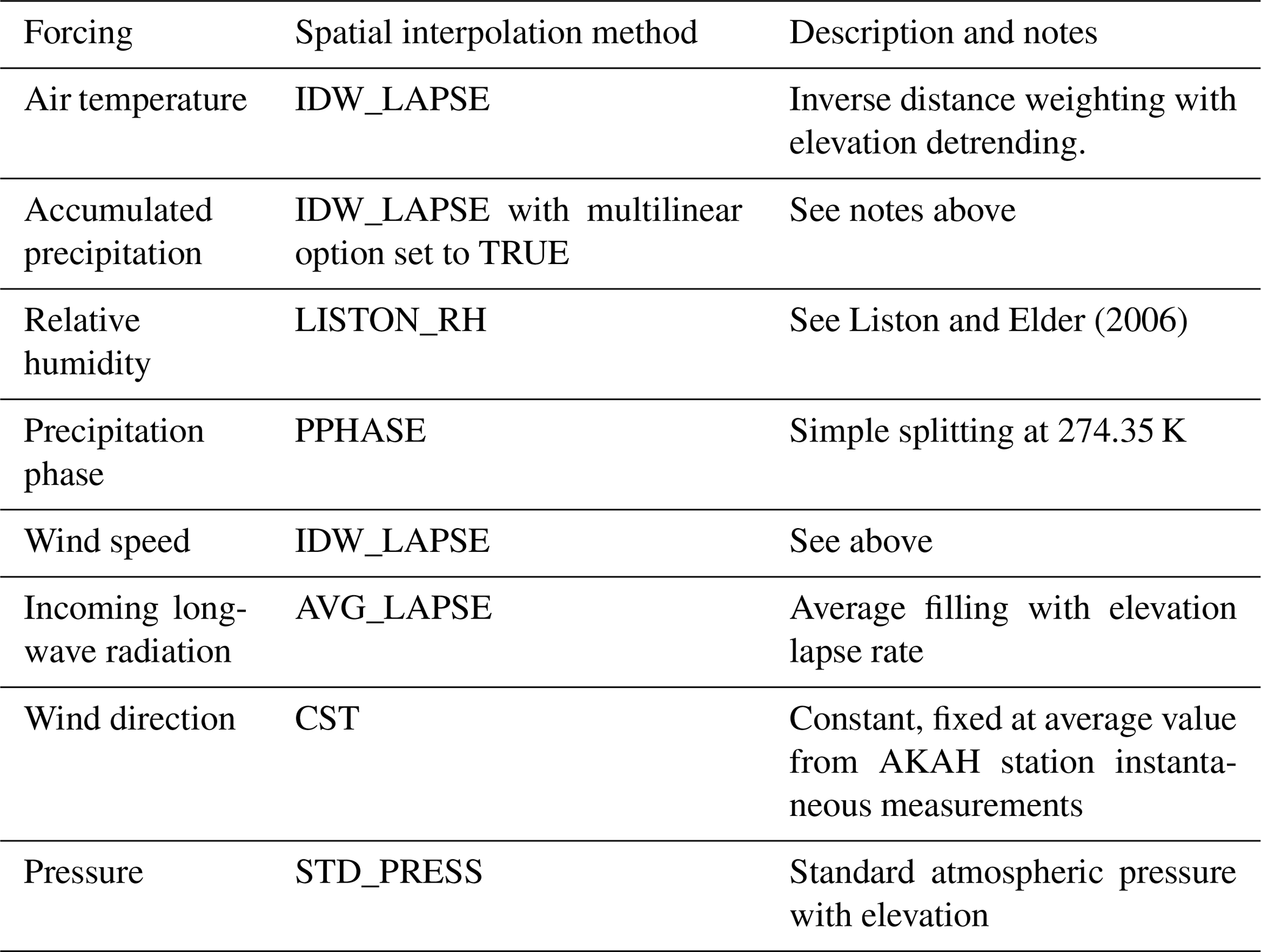
The forcings were hourly for the following measurements: incoming shortwave, incoming longwave, air temperature, relative humidity, wind speed, wind direction, reflected shortwave, accumulated precipitation, and ground temperature.
Critical to Alpine3D are the interpolation methods from MeteoIO to spatially distribute precipitation and other forcings. We found the modeled SWE to be highly dependent on the spatial interpolation of precipitation. Our initial approach was to explore local (i.e., with a given radius from a station) and regional (i.e., all AKAH stations) lapse rates in the measured snow depth and modeled precipitation from SNOWPACK. We found almost no correlation in many of the measurements, which was not surprising given the complexity of the terrain and likely existence of microclimates with substantial influence on precipitation. Without having a good validation source for spatial precipitation (as is the case for all of High Mountain Asia), we selected an interpolation method that yielded relatively smooth results but showed increases in precipitation with elevation.
Ultimately, we decided to use an inverse distance weighting scheme with elevation detrending (IDW_LAPSE) and a multilinear option. For this method, the input data are detrended, and then the residuals are spatially interpolated according to an inverse distance weighting scheme. The detrending uses a multiple linear regression with northing, easting, and altitude. The linear regression has an iterative method for removing outliers. Finally, values at each cell are retrended using the multiple linear regression and added to the interpolated residuals.
A summary of the interpolation methods, all of which are defined in the MeteoIO documentation (Bavay and Egger, 2014), is given in Table A3.
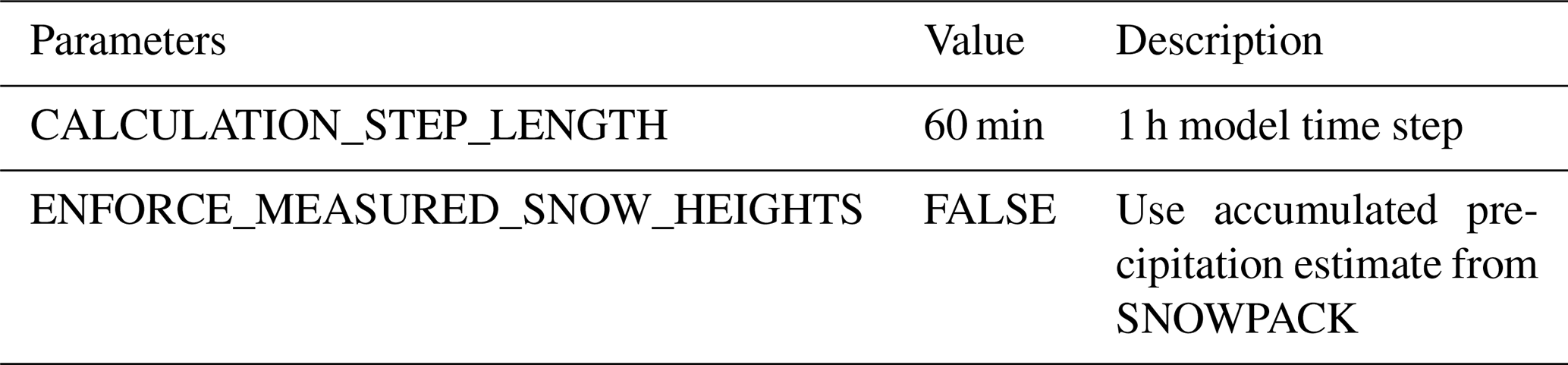
The same parameters as in Table A2 for SNOWPACK were used in Alpine3D, with changes shown in Table A4. Other parameters were defaults.
The code for ParBal is accessible at https://github.com/edwardbair/ParBal (Bair et al., 2019a).
The codes for MeteoIO (https://models.slf.ch/p/meteoio/, Bavay et al., 2015a), SNOWPACK (https://models.slf.ch/p/snowpack/, Bavay et al., 2015b), and Alpine3D (https://models.slf.ch/p/alpine3d/, Bavay et al., 2015c) are accessible at https://models.slf.ch/.
The code for Noah-MP is accessible at https://ral.ucar.edu/solutions/products/noah-multiparameterization-land-surface-model-noah-mp-lsm (Niu and Yange, 2015).
The GLDAS-2 (https://doi.org/10.5067/L0JGCNVBNRAX, Beaudoing and Rodell, 2015) and MERRA-2 (https://doi.org/10.5067/VJAFPLI1CSIV, GMAO, 2015) forcings are accessible at https://disc.gsfc.nasa.gov/.
The reconstructed SWE and melt cubes are accessible at ftp://ftp.snow.ucsb.edu/pub/org/snow/products/reconstruction/h23v05/500m/ (Bair, 2019).
Unfortunately, the AKAH measurements are not publicly available due to security concerns. Requests for the dataset should be made through the Aga Khan Agency for Habitat (https://www.akdn.org, last access: May 2019).
The supplement related to this article is available online at: https://doi.org/10.5194/tc-14-331-2020-supplement.
DC provided the AKAH dataset. JA ran the Noah-MP simulations. KR prepared the snow surface properties dataset. EB processed the data and prepared the paper.
The authors declare that they have no conflict of interest.
We are grateful to the Aga Khan Agency for Habitat for supplying the first snow measurements in Afghanistan's watersheds since the 1980s. We thank Jürg Schweizer and two anonymous referees for their reviews.
This research has been supported by the National Aeronautics and Space Administration (grant nos. 80NSSC18K0427, 80NSSC18K1489, 2015 HiMAT, and NNX17AC15G).
This paper was edited by Jürg Schweizer and reviewed by two anonymous referees.
Adam, J. C., Clark, E. A., Lettenmaier, D. P., and Wood, E. F.: Correction of global precipitation products for orographic effects, J. Clim., 19, 15–38, https://doi.org/10.1175/JCLI3604.1, 2006.
Armstrong, R. L., Rittger, K., Brodzik, M. J., A. Racoviteanu, Barrett, A. P., Singh Khalsa, S.-J., Raup, B., Hill, A. F., Khan, A. L., Wilson, A. M., Bhakta Kayastha, R., Fetterer, F., and Armstrong, B.: Runoff from glacier ice and seasonal snow in High Asia: separating melt water sources in river flow Reg. Environ. Change, 19, 1249–1261, https://doi.org/10.1007/s10113-018-1429-0, 2018.
Bair, E. H.: Reconstructed SWE and melt for MODIS tile h23v05, available at: ftp://ftp.snow.ucsb.edu/pub/org/snow/products/reconstruction/h23v05/500m/, 2019.
Bair, E. H., Simenhois, R., Birkeland, K., and Dozier, J.: A field study on failure of storm snow slab avalanches, Cold Reg. Sci. Technol., 79–80, 20–28, https://doi.org/10.1016/j.coldregions.2012.02.007, 2012.
Bair, E. H., Rittger, K., Davis, R. E., Painter, T. H., and Dozier, J.: Validating reconstruction of snow water equivalent in California's Sierra Nevada using measurements from the NASA Airborne Snow Observatory, Water Resour. Res., 52, 8437–8460, https://doi.org/10.1002/2016WR018704, 2016.
Bair, E. H., Abreu Calfa, A., Rittger, K., and Dozier, J.: Using machine learning for real-time estimates of snow water equivalent in the watersheds of Afghanistan, The Cryosphere, 12, 1579–1594, https://doi.org/10.5194/tc-12-1579-2018, 2018a.
Bair, E. H., Davis, R. E., and Dozier, J.: Hourly mass and snow energy balance measurements from Mammoth Mountain, CA USA, 2011–2017, Earth Syst. Sci. Data, 10, 549–563, https://doi.org/10.5194/essd-10-549-2018, 2018b.
Bair, E. H., Rittger, K., and Dozier, J.: The Parallel Energy Balance Model source code, available at: https://github.com/edwardbair/ParBal, 2019a.
Bair, E. H., Rittger, K., Skiles, S. M., and Dozier, J.: An Examination of Snow Albedo Estimates From MODIS and Their Impact on Snow Water Equivalent Reconstruction, Water Resour. Res., 55, 7826–7842, https://doi.org/10.1029/2019wr024810, 2019b.
Bartelt, P. and Lehning, M.: A physical SNOWPACK model for the Swiss avalanche warning: Part I: numerical model, Cold Reg. Sci. Technol., 35, 123–145, https://doi.org/10.1016/s0165-232x(02)00074-5, 2002.
Bavay, M. and Egger, T.: MeteoIO 2.4.2: a preprocessing library for meteorological data, Geosci. Model Dev., 7, 3135–3151, https://doi.org/10.5194/gmd-7-3135-2014, 2014.
Bavay, M., Egger, T., Michel, A., and Reisecker, M.: MeteoIO source code, available at: https://models.slf.ch/p/meteoio/, 2019a.
Bavay, M., C. Fierz Hirashima, H., Wever, N., Richter, B., Michel, A., and Ebner, P.: SNOWPACK source code, available at: https://models.slf.ch/p/snowpack/, 2019b.
Bavay, M., Fierz, C., Wever, N., and Michel, A.: Alpine3D source code, available at: https://models.slf.ch/p/alpine3d/, 2019c.
Beaudoing, H. and Rodell, M.: NASA/GSFC/HSL (2015), GLDAS Noah Land Surface Model L4 3 hourly 1.0 × 1.0 degree V2.0, Greenbelt, Maryland, USA, Goddard Earth Sciences Data and Information Services Center (GES DISC), https://doi.org/10.5067/L0JGCNVBNRAX, last accessed: May 2015.
Bedford, D. and Tsarev, B.: Central Asian Snow Cover from Hydrometeorological Surveys, Version 1, Boulder, Colorado USA, NSIDC: National Snow and Ice Data Center, https://doi.org/10.7265/N51Z4291, 2001.
Bellaire, S., Jamieson, J. B., and Fierz, C.: Forcing the snow-cover model SNOWPACK with forecasted weather data, The Cryosphere, 5, 1115–1125, https://doi.org/10.5194/tc-5-1115-2011, 2011.
Bellaire, S., van Herwijnen, A., Bavay, M., and Schweizer, J.: Distributed modeling of snow cover instability at regional scale, Proceedings of the 2018 International Snow Science Workshop, Innsbruck, Austria, 871–875, 2018.
Bookhagen, B. and Burbank, D. W.: Toward a complete Himalayan hydrological budget: Spatiotemporal distribution of snowmelt and rainfall and their impact on river discharge, J. Geophys. Res.-Ea. Surf., 115, F03019, https://doi.org/10.1029/2009jf001426, 2010.
Broxton, P. D., Zeng, X., and Dawson, N.: Why Do Global Reanalyses and Land Data Assimilation Products Underestimate Snow Water Equivalent?, J. Hydrometeorol., 17, 2743–2761, https://doi.org/10.1175/jhm-d-16-0056.1, 2016.
Burt, P. and Adelson, E.: The Laplacian pyramid as a compact image code, IEEE Transactions on Communications, 31, 532–540, https://doi.org/10.1109/TCOM.1983.1095851, 1983.
Chabot, D. and Kaba, A.: Avalanche forecasting in the central Asian countries of Afghanistan, Pakistan and Tajikistan, Proc. 2016 Intl. Snow Sci. Wksp., Breckenridge, CO, 2016.
Chen, F., Barlage, M., Tewari, M., Rasmussen, R., Jin, J., Lettenmaier, D., Livneh, B., Lin, C., Miguez-Macho, G., Niu, G.-Y., Wen, L., and Yang, Z.-L.: Modeling seasonal snowpack evolution in the complex terrain and forested Colorado Headwaters region: A model intercomparison study, J. Geophys. Res.-Atmos., 119, 13795–13819, https://doi.org/10.1002/2014jd022167, 2014.
Cornwell, E., Molotch, N. P., and McPhee, J.: Spatio-temporal variability of snow water equivalent in the extra-tropical Andes Cordillera from distributed energy balance modeling and remotely sensed snow cover, Hydrol. Earth Syst. Sci., 20, 411–430, https://doi.org/10.5194/hess-20-411-2016, 2016.
Cosgrove, B. A., Lohmann, D., Mitchell, K. E., Houser, P. R., Wood, E. F., Schaake, J. C., Robock, A., Marshall, C., Sheffield, J., Duan, Q., Luo, L., Higgins, R. W., Pinker, R. T., Tarpley, J. D., and Meng, J.: Real-time and retrospective forcing in the North American Land Data Assimilation System (NLDAS) project, J. Geophys. Res.-Atmos., 108, 8842, https://doi.org/10.1029/2002JD003118, 2003.
Dahri, Z. H., Ludwig, F., Moors, E., Ahmad, B., Khan, A., and Kabat, P.: An appraisal of precipitation distribution in the high-altitude catchments of the Indus basin, Sci. Total Environ., 548–549, 289–306, https://doi.org/10.1016/j.scitotenv.2016.01.001, 2016.
Dahri, Z. H., Moors, E., Ludwig, F., Ahmad, S., Khan, A., Ali, I., and Kabat, P.: Adjustment of measurement errors to reconcile precipitation distribution in the high-altitude Indus basin, Int. J. Climatol., 38, 3842–3860, https://doi.org/10.1002/joc.5539, 2018.
Dozier, J. and Frew, J.: Rapid calculation of terrain parameters for radiation modeling from digital elevation data, IEEE T. Geosci. Remote, 28, 963–969, https://doi.org/10.1109/36.58986, 1990.
Dozier, J., Painter, T. H., Rittger, K., and Frew, J. E.: Time-space continuity of daily maps of fractional snow cover and albedo from MODIS, Adv. Water Res., 31, 1515–1526, https://doi.org/10.1016/j.advwatres.2008.08.011, 2008.
Ek, M. B., Mitchell, K. E., Lin, Y., Rogers, E., Grunmann, P., Koren, V., Gayno, G., and Tarpley, J. D.: Implementation of Noah land surface model advances in the National Centers for Environmental Prediction operational mesoscale Eta model, J. Geophys. Res.-Atmos., 108, 8851, https://doi.org/10.1029/2002jd003296, 2003.
Fierz, C., Armstrong, R. L., Durand, Y., Etchevers, P., Greene, E., McClung, D. M., Nishimura, K., Satyawali, P. K., and Sokratov, S.: The International Classification for Seasonal Snow on the Ground, IHP-VII Technical Documents in Hydrology N∘83, 90, 2009.
Gelaro, R., McCarty, W., Suárez, M. J., Todling, R., Molod, A., Takacs, L., Randles, C. A., Darmenov, A., Bosilovich, M. G., Reichle, R., Wargan, K., Coy, L., Cullather, R., Draper, C., Akella, S., Buchard, V., Conaty, A., Silva, A. M. D., Gu, W., Kim, G.-K., Koster, R., Lucchesi, R., Merkova, D., Nielsen, J. E., Partyka, G., Pawson, S., Putman, W., Rienecker, M., Schubert, S. D., Sienkiewicz, M., and Zhao, B.: The Modern-Era Retrospective Analysis for Research and Applications, Version 2 (MERRA-2), J. Clim., 30, 5419–5454, https://doi.org/10.1175/jcli-d-16-0758.1, 2017.
Global Modeling and Assimilation Office (GMAO): MERRA-2, Greenbelt, MD, USA, Goddard Earth Sciences Data and Information Services Center (GES DISC), https://doi.org/10.5067/VJAFPLI1CSIV, last access: May 2015.
Goodison, B., Louie, P. Y. T., and Yang, D.: WMO Solid precipitation measurement intercomparison, World Meteorological Organization, 1998.
Harris, I., Jones, P. D., Osborn, T. J., and Lister, D. H.: Updated high-resolution grids of monthly climatic observations – the CRU TS3.10 Dataset, Int. J. Climatol., 34, 623–642, https://doi.org/10.1002/joc.3711, 2014.
Hirashima, H., Yamaguchi, S., Sato, A., and Lehning, M.: Numerical modeling of liquid water movement through layered snow based on new measurements of the water retention curve, Cold Reg. Sci. Technol., 64, 94–103, https://doi.org/10.1016/j.coldregions.2010.09.003, 2010.
Huffman, G. J., Bolvin, D. T., Nelkin, E. J., Wolff, D. B., Adler, R. F., Gu, G., Hong, Y., Bowman, K. P., and Stocker, E. F.: The TRMM Multisatellite Precipitation Analysis (TMPA): Quasi-Global, Multiyear, Combined-Sensor Precipitation Estimates at Fine Scales, J. Hydrometeorol., 8, 38–55, https://doi.org/10.1175/jhm560.1, 2007.
Immerzeel, W. W., Wanders, N., Lutz, A. F., Shea, J. M., and Bierkens, M. F. P.: Reconciling high-altitude precipitation in the upper Indus basin with glacier mass balances and runoff, Hydrol. Earth Syst. Sci., 19, 4673–4687, https://doi.org/10.5194/hess-19-4673-2015, 2015.
Jamieson, J. B.: The compression test – after 25 years, The Avalanche Review, 18, 10–12, 1999.
Jepsen, S. M., Molotch, N. P., Williams, M. W., Rittger, K. E., and Sickman, J. O.: Interannual variability of snowmelt in the Sierra Nevada and Rocky Mountains, United States: Examples from two alpine watersheds, Water Resour. Res., 48, W02529, https://doi.org/10.1029/2011WR011006, 2012.
Kochendorfer, J., Rasmussen, R., Wolff, M., Baker, B., Hall, M. E., Meyers, T., Landolt, S., Jachcik, A., Isaksen, K., Brækkan, R., and Leeper, R.: The quantification and correction of wind-induced precipitation measurement errors, Hydrol. Earth Syst. Sci., 21, 1973–1989, https://doi.org/10.5194/hess-21-1973-2017, 2017.
Lehning, M., Bartelt, P., Brown, B., Russi, T., Stöckli, U., and Zimmerli, M.: SNOWPACK model calculations for avalanche warning based upon a new network of weather and snow stations, Cold Reg. Sci. Technol., 30, 145–157, 1999.
Lehning, M., Bartelt, P., Brown, B., and Fierz, C.: A physical SNOWPACK model for the Swiss avalanche warning: Part III: meteorological forcing, thin layer formation and evaluation, Cold Reg. Sci. Technol., 35, 169–184, https://doi.org/10.1016/S0165-232X(02)00072-1, 2002a.
Lehning, M., Bartelt, P., Brown, B., Fierz, C., and Satyawali, P.: A physical SNOWPACK model for the Swiss avalanche warning, Part II: Snow microstructure, Cold Reg. Sci. Technol., 35, 147–167, https://doi.org/10.1016/S0165-232X(02)00073-3, 2002b.
Lehning, M., Völksch, I., Gustafsson, D., Nguyen, T. A., Stähli, M., and Zappa, M.: ALPINE3D: a detailed model of mountain surface processes and its application to snow hydrology, Hydrol. Process., 20, 2111–2128, https://doi.org/10.1002/hyp.6204, 2006.
Liston, G. E. and Elder, K.: A meteorological distribution system for high-resolution terrestrial modeling (MicroMet), J. Hydrometeorol., 7, 217–234, https://doi.org/10.1175/JHM486.1, 2006.
Lutz, A. F., Immerzeel, W. W., Shrestha, A. B., and Bierkens, M. F. P.: Consistent increase in High Asia's runoff due to increasing glacier melt and precipitation, Nature Climate Change, 4, 587, https://doi.org/10.1038/nclimate2237, 2014.
Margulis, S. A., Cortés, G., Girotto, M., and Durand, M.: A Landsat-Era Sierra Nevada Snow Reanalysis (1985–2015), J. Hydrometeorol., 17, 1203–1221, https://doi.org/10.1175/jhm-d-15-0177.1, 2016.
Marks, D. and Dozier, J.: Climate and energy exchange at the snow surface in the alpine region of the Sierra Nevada, 2, Snow cover energy balance, Water Resour. Res., 28, 3043–3054, https://doi.org/10.1029/92WR01483, 1992.
Martinec, J. and Rango, A.: Areal distribution of snow water equivalent evaluated by snow cover monitoring, Water Resour. Res., 17, 1480–1488, https://doi.org/10.1029/WR017i005p01480, 1981.
Milly, P. C. D. and Dunne, K. A.: Macroscale water fluxes 1. Quantifying errors in the estimation of basin mean precipitation, Water Resour. Res., 38, 23-21-23-14, https://doi.org/10.1029/2001WR000759, 2002.
Mitterer, C. and Schweizer, J.: Analysis of the snow-atmosphere energy balance during wet-snow instabilities and implications for avalanche prediction, The Cryosphere, 7, 205–216, https://doi.org/10.5194/tc-7-205-2013, 2013.
Molotch, N. P.: Reconstructing snow water equivalent in the Rio Grande headwaters using remotely sensed snow cover data and a spatially distributed snowmelt model, Hydrol. Process., 23, 1076–1089, https://doi.org/10.1002/hyp.7206, 2009.
Monti, F., Schweizer, J., and Fierz, C.: Hardness estimation and weak layer detection in simulated snow stratigraphy, Cold Reg. Sci. Technol., 103, 82–90, https://doi.org/10.1016/j.coldregions.2014.03.009, 2014.
Nishimura, K., Baba, E., Hirashima, H., and Lehning, M.: Application of the snow cover model SNOWPACK to snow avalanche warning in Niseko, Japan, Cold Reg. Sci. Technol., 43, 62–70, https://doi.org/10.1016/j.coldregions.2005.05.007, 2005.
Niu, G.-Y. and Yang, Z.-L.: Effects of vegetation canopy processes on snow surface energy and mass balances, J. Geophys. Res.-Atmos., 109, D23111, https://doi.org/10.1029/2004jd004884, 2004.
Niu, G.-Y. and Yange, Z.-L.: Noah-MP source code, available at: https://ral.ucar.edu/solutions/products/noah-multiparameterization-land-surface-model-noah-mp-lsm, 2015.
Niu, G.-Y., Yang, Z.-L., Mitchell, K. E., Chen, F., Ek, M. B., Barlage, M., Kumar, A., Manning, K., Niyogi, D., Rosero, E., Tewari, M., and Xia, Y.: The community Noah land surface model with multiparameterization options (Noah-MP): 1. Model description and evaluation with local-scale measurements, J. Geophys. Res.-Atmos., 116, https://doi.org/10.1029/2010jd015139, 2011. surface energy and mass balances, J. Geophys. Res.-Atmos., 109, https://doi.org/10.1029/2004jd004884, 2004.
Painter, T. H., Rittger, K., McKenzie, C., Slaughter, P., Davis, R. E., and Dozier, J.: Retrieval of subpixel snow-covered area, grain size, and albedo from MODIS, Remote Sens. Environ., 113, 868–879, https://doi.org/10.1016/j.rse.2009.01.001, 2009.
Painter, T. H., Bryant, A. C., and Skiles, S. M.: Radiative forcing by light absorbing impurities in snow from MODIS surface reflectance data, Geophys. Res. Lett., 39, L17502, https://doi.org/10.1029/2012GL052457, 2012.
Painter, T. H., Berisford, D. F., Boardman, J. W., Bormann, K. J., Deems, J. S., Gehrke, F., Hedrick, A., Joyce, M., Laidlaw, R., Marks, D., Mattmann, C., McGurk, B., Ramirez, P., Richardson, M., Skiles, S. M., Seidel, F. C., and Winstral, A.: The Airborne Snow Observatory: Fusion of scanning lidar, imaging spectrometer, and physically-based modeling for mapping snow water equivalent and snow albedo, Remote Sens. Environ., 184, 139–152, https://doi.org/10.1016/j.rse.2016.06.018, 2016.
Raup, B., Racoviteanu, A., Khalsa, S. J. S., Helm, C., Armstrong, R., and Arnaud, Y.: The GLIMS geospatial glacier database: A new tool for studying glacier change, Global Planet. Change, 56, 101–110, https://doi.org/10.1016/j.gloplacha.2006.07.018, 2007.
Rienecker, M. M., Suarez, M. J., Gelaro, R., Todling, R., Julio Bacmeister, Liu, E., Bosilovich, M. G., Schubert, S. D., Takacs, L., Kim, G.-K., Bloom, S., Chen, J., Collins, D., Conaty, A., Silva, A. d., Gu, W., Joiner, J., Koster, R. D., Lucchesi, R., Molod, A., Owens, T., Pawson, S., Pegion, P., Redder, C. R., Reichle, R., Robertson, F. R., Ruddick, A. G., Sienkiewicz, M., and Woollen, J.: MERRA: NASA's Modern-Era Retrospective Analysis for Research and Applications, J. Clim., 24, 3624–3648, https://doi.org/10.1175/jcli-d-11-00015.1, 2011.
Rittger, K., Bair, E. H., Kahl, A., and Dozier, J.: Spatial estimates of snow water equivalent from reconstruction, Adv. Water Res., 94, 345–363, https://doi.org/10.1016/j.advwatres.2016.05.015, 2016.
Rittger, K., Raleigh, M. S., Dozier, J., Hill, A. F., Lutz, J. A., and Painter, T. H.: Canopy Adjustment and Improved Cloud Detection for Remotely Sensed Snow Cover Mapping, Water Resour. Res., in press, 2020.
Rodell, M., Houser, P. R., Jambor, U., Gottschalck, J., Mitchell, K., Meng, C. J., Arsenault, K., Cosgrove, B., Radakovich, J., Bosilovich, M., Entin, J. K., Walker, J. P., Lohmann, D., and Toll, D.: The Global Land Data Assimilation System, B. Am. Meteorol. Soc., 85, 381–394, https://doi.org/10.1175/BAMS-85-3-381, 2004.
Rutan, D. A., Kato, S., Doelling, D. R., Rose, F. G., Nguyen, L. T., Caldwell, T. E., and Loeb, N. G.: CERES synoptic product: Methodology and validation of surface radiant flux, J. Atmos. Ocean. Technol., 32, 1121–1143, https://doi.org/10.1175/JTECH-D-14-00165.1, 2015.
Schweizer, J. and Jamieson, B.: Snow cover properties for skier triggering of avalanches, Cold Reg. Sci. Technol., 33, 207–221, https://doi.org/10.1016/s0165-232x(01)00039-8, 2001.
Schweizer, J. and Jamieson, B.: A threshold sum approach to stability evaluation of manual snow profiles, Cold Reg. Sci. Technol., 47, 50–59, https://doi.org/10.1016/j.coldregions.2006.08.011, 2007.
Shakoor, A. and Ejaz, N.: Flow Analysis at the Snow Covered High Altitude Catchment via Distributed Energy Balance Modeling, Scientific Reports, 9, 4783, https://doi.org/10.1038/s41598-019-39446-1, 2019.
Skiles, S. M. and Painter, T.: Daily evolution in dust and black carbon content, snow grain size, and snow albedo during snowmelt, Rocky Mountains, Colorado, J. Glaciol., 63, 118–132, https://doi.org/10.1017/jog.2016.125, 2016.
Smith, T. and Bookhagen, B.: Changes in seasonal snow water equivalent distribution in High Mountain Asia (1987 to 2009), Sci. Adv., 4, e1701550, https://doi.org/10.1126/sciadv.1701550, 2018.
Sturm, M., Holmgren, J., and Liston, G. E.: A seasonal snow cover classification system for local to global applications, J. Clim., 8, 1261–1283, https://doi.org/10.1175/1520-0442(1995)008<1261:ASSCCS>2.0.CO;2, 1995.
Sturm, M., Taras, B., Liston, G. E., Derksen, C., Jonas, T., and Lea, J.: Estimating snow water equivalent using snow depth data and climate classes, J. Hydrometeorol., 11, 1380–1394, https://doi.org/10.1175/2010jhm1202.1, 2010.
Tan, B., Woodcock, C. E., Hu, J., Zhang, P., Ozdogan, M., Huang, D., Yang, W., Knyazikhin, Y., and Myneni, R. B.: The impact of gridding artifacts on the local spatial properties of MODIS data: Implications for validation, compositing, and band-to-band registration across resolutions, Remote Sens. Environ., 105, 98–114, https://doi.org/10.1016/j.rse.2006.06.008, 2006.
United Nations: Afghanistan: Nuristan avalanche, update to flash report (as of 8 February 2017), Office for the Coordination of Humanitarian Affairs (OCHA), 2017.
USAID: Afghanistan Food Security Update, FEWS Net, Washington, DC, 4, 2008.
USGS: Global Land Survey, Sioux Falls, SD: Land Processes DAAC, retrieved from http://glcfapp.glcf.umd.edu/data/gls/ (last access: 15 May 201), 2009.
van Herwijnen, A. and Jamieson, B.: Fracture character in compression tests, Cold Reg. Sci. Technol., 47, 60–68, https://doi.org/10.1016/j.coldregions.2006.08.016, 2007.
Viste, E. and Sorteberg, A.: Snowfall in the Himalayas: an uncertain future from a little-known past, The Cryosphere, 9, 1147–1167, https://doi.org/10.5194/tc-9-1147-2015, 2015.
Xia, Y., Mitchell, K., Ek, M., Sheffield, J., Cosgrove, B., Wood, E., Luo, L., Alonge, C., Wei, H., Meng, J., Livneh, B., Lettenmaier, D., Koren, V., Duan, Q., Mo, K., Fan, Y., and Mocko, D.: Continental-scale water and energy flux analysis and validation for the North American Land Data Assimilation System project phase 2 (NLDAS-2): 1. Intercomparison and application of model products, J. Geophys. Res.-Atmos., 117, D03109, https://doi.org/10.1029/2011JD016048, 2012.
Xiaoxiong, X., Nianzeng, C., and Barnes, W.: Terra MODIS on-orbit spatial characterization and performance, IEEE T. Geosci. Remote, 43, 355–365, https://doi.org/10.1109/TGRS.2004.840643, 2005.
Yang, Z.-L. and Niu, G.-Y.: The Versatile Integrator of Surface and Atmosphere processes: Part 1. Model description, Global Planet. Change, 38, 175–189, https://doi.org/10.1016/S0921-8181(03)00028-6, 2003.
Yatagai, A., Kamiguchi, K., Arakawa, O., Hamada, A., Yasutomi, N., and Kitoh, A.: APHRODITE: Constructing a Long-Term Daily Gridded Precipitation Dataset for Asia Based on a Dense Network of Rain Gauges, B. Am. Meteorol. Soc., 93, 1401–1415, https://doi.org/10.1175/bams-d-11-00122.1, 2012.
- Abstract
- Introduction
- Aga Khan Agency for Habitat (AKAH) stations
- Literature review
- Previous work with AKAH snow measurements
- Methods
- Results and discussion
- Conclusions
- Appendix A: Detailed model forcings and parameters
- Code and data availability
- Author contributions
- Competing interests
- Acknowledgements
- Financial support
- Review statement
- References
- Supplement