the Creative Commons Attribution 4.0 License.
the Creative Commons Attribution 4.0 License.
 | 05 Feb 2020
Effects of decimetre-scale surface roughness on L-band brightness temperature of sea ice
Maciej Miernecki
Lars Kaleschke
Nina Maaß
Stefan Hendricks
Sten Schmidl Søbjærg
Sea ice thickness is an essential climate variable. Current L-Band sea ice thickness retrieval methods do not account for sea ice surface roughness that is hypothesised to be not relevant to the process. This study attempts to validate this hypothesis that has not been tested yet. To test this hypothesis, we created a physical model of sea ice roughness based on geometrical optics and merged it into the L-band emissivity model of sea ice that is similar to the one used in the operational sea ice thickness retrieval algorithm. The facet description of sea ice surface used in geometrical optics is derived from 2-D surface elevation measurements. Subsequently the new model was tested with TB measurements performed during the SMOSice 2014 field campaign. Our simulation results corroborate the hypothesis that sea ice surface roughness has a marginal impact on near-nadir TB (used in the current operational retrieval). We demonstrate that the probability distribution function of surface slopes can be approximated with a parametric function whose single parameter can be used to characterise the degree of roughness. Facet azimuth orientation is isotropic at scales greater than 4.3 km. The simulation results indicate that surface roughness is a minor factor in modelling the sea ice brightness temperature. The change in TB is most pronounced at incidence angles greater than 40∘ and can reach up to 8 K for vertical polarisation at 60∘. Therefore current and future L-band missions (SMOS, SMAP, CIMR, SMOS-HR) measuring at such angles can be affected. Comparison of the brightness temperature simulations with the SMOSice 2014 radiometer data does not yield definite results.


The L-band brightness temperature (TB) is sensitive to sea ice thickness. This feature is used for sea ice thickness retrieval from L-band TB (over thin ice, < 1.5 m) (Tian-Kunze et al., 2014; Huntemann et al., 2014; Kaleschke et al., 2016). Several factors influence TB measurements over ice-covered regions, among them ice concentration, ice temperature, snow cover, sea ice surface roughness, and the shape of the interfaces between the snow and ice layers (Maaß et al., 2013; Ulaby et al., 2014, p. 422).
Here, we investigate the effects of surface roughness on the L-band TB, specifically the large-scale roughness. So far this factor is not included in the modelling of sea ice emissions in operational sea ice thickness retrieval. Electromagnetic scattering theory assumes that the roughness of a random surface is characterised by statistical parameters including standard deviation of surface height (σz) and correlation function (R(ξ)) measured in units of wavelength (Ulaby et al., 2014, p. 422). These roughness statistical parameters are derived from measurements of surface elevation (z), conducted with altimeters that are characterised by their accuracy (δ) and sampling distance (Δx). As usual, the measurement method has an impact on the outcome, in this case by filtering out both high and low spatial frequencies of the surface roughness. Sea ice elevation measurements obtained from airborne altimeters (Ketchum, 1971; Dierking, 1995) and supplemented with terrestrial laser scanners (Landy et al., 2015) draw a picture of sea ice roughness as a multi-scale feature covering several orders of magnitude from large floes and pressure ridges (from tens to hundreds of metres) to frost flowers and small ripples (on the centimetre to millimetre scale). The incident radiation of a given wavelength (λ) reacts differently with individual components of the superimposed roughness of many scales (Ulaby et al., 2014, p. 252).
At small end of the roughness spectrum i.e. when the change of surface elevation over sampling distance (Δz∕Δx) is much smaller than λ (), the surface roughness is negligible. It means that the angular characteristics of scattered radiation are the same as for the secular surface. As a rule of thumb, Δx should be smaller than 0.1λ (Dierking, 2000). Sea ice roughness measurements with terrestrial lidar carried out by Landy et al. (2015) show that standard deviation of surface height σz ranges from 0.001 to 0.0064 m, after high-pass filtering (cut-off at 4 m−1, Δx=0.002 m). These results indicate that, according to the Fraunhofer's smoothness criterion (, where θ is the angle of incidence), most sea ice types (except artificially grown frost flowers) can be treated as a smooth surface for the L-band at scales lower than 0.25 m.
In this study, we focus on the other side of the roughness spectrum, i.e. the large-scale surface roughness of sea ice (). In this case, changes in surface elevation are not negligible and alter the local incidence angle (θi). Studies of surface scattering by Lawrence et al. (2011, 2013) conclude that region of 8λ×8λ is sufficient to model small-scale roughness. Here, we assume that at larger spatial scales (larger than 8λ×8λ) the surface roughness can be characterised in terms of geometrical optics (GO), for sea ice with ϵice=4.1, m.
GO approximation describes the surface as a set of facets (Ulaby et al., 2014, pages 564–567). This approach was applied for modelling the effective emissivities of mountainous terrain (Matzler and Standley, 2000) and ocean surface (Prigent and Abba, 1990). The last study involved probability distribution of slopes in crosswind and downwind directions. A similar method was used in the context of sea ice to assess the uncertainties caused by roughness in sea ice concentration products derived from passive microwaves (Stroeve et al., 2006). Liu et al. (2014) measured ice surface slopes and other roughness statistics in the Bohai Sea. Their result was obtained with linear (1-D) scans under the assumption of isotropic roughness characteristics. The study by Beckers et al. (2015) has demonstrated that the statistics of sea ice roughness (mean z, σz, kurtosis, and skewness) obtained from 1-D altimeter and 2-D laser scanner converge, on the condition that the surface is not strongly heterogeneous. Nonetheless, the 1-D altimeter data cannot properly represent the spatial orientation of surface facets. The surface facet orientation is characterised by both the slope (α) and the azimuthal angle in which it is facing (γ).
In this paper, we address the knowledge gap regarding the influence of large-scale surface roughness on L-band TB. The paper comprises four main sections. The introduction, presenting the context, is in Sect. 1.
Section 2 introduces the experimental data collected during the SMOSice 2014 campaign (Sect. 2.1). Among them are the EMIRAD2 L-band radiometer TB measurements, which will serve as a reference for the TB simulations. Another instrument is the airborne laser scanner (ALS) used for surface elevation measurements. The surface elevation measurements are used to construct a digital elevation model (DEM) of sea ice surface. From the DEM we derive the facet surface slopes and their orientation. In Sect. 2.2 we analyse the statistics of the facet orientation. Based on facet orientation statistics, we derive a parameterisation of the probability distribution function of surface slopes (PDFα), which will serve as surface roughness representation in TB simulations.
Section 2.3 presents the setup used for sea ice TB simulation. For the simulation of the sea ice TB we use the MIcrowave L-band LAyered Sea ice emission model (MILLAS) (Maaß et al., 2013). In Sect. 2.4 we show how we integrate the surface roughness statistics (PDFα) with MILLAS using geometrical optics.
The three key results of this study, namely that (a) surface roughness reduces the polarisation difference, this change being most pronounced at incidence angles greater than 50∘; (b) nadir TB is little affected; and (c) comparison with the radiometer data and sensitivity study indicates that snow cover has a greater impact on the TB than surface roughness, are subsequently presented and discussed in Sect. 3.
Section 4 summarises the results and discusses the implications of this study for current and future L-band missions.
In this section we present the SMOSice 2014 campaign that is the key dataset of this study (Sect. 2.1). Section 2.2 presents the sea ice surface roughness measurements in the context of geometrical optics. Section 2.3 presents the sea ice emission model that we used.
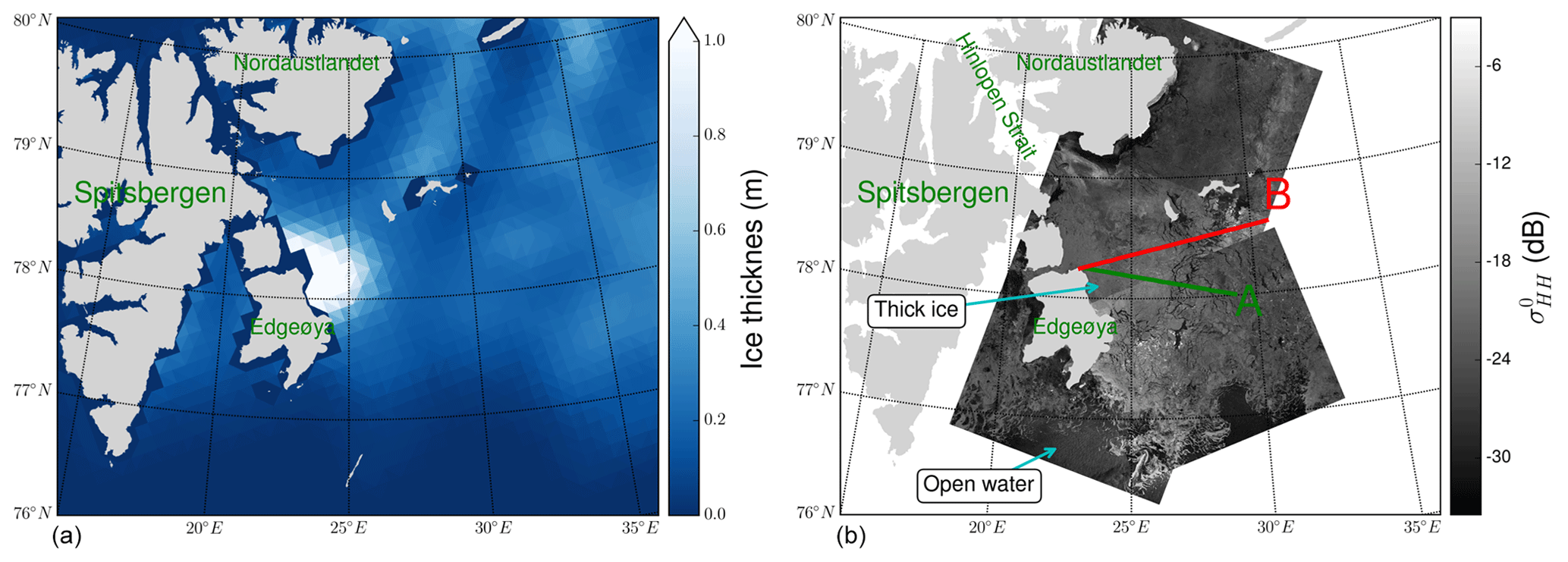
Figure 1The region of the SMOSice 2014 campaign. (a) Sea ice thickness on 24 March 2014, derived from SMOS. The SMOS sea ice thickness product with a resolution of 40 km is presented on a 15 km grid. An aggregation of thick ice (> 1 m) is visible along the Edgeøya's eastern coast. (b) The TerraSAR-X wide-swath mode (HH polarisation), with frames taken at 05:35 and 14:58 UTC. The aircraft tracks are marked in green (A) at 10:05–10:41 UTC and red (B) at 11:25–12:07 UTC.
2.1 SMOSice 2014 campaign
The SMOSice 2014 campaign took place between 21 and 27 March 2014 in the area between Edgeøya and Kong Karls Land, east of Svalbard. Hendricks et al. (2014) and Kaleschke et al. (2016) described the campaign extensively. In this study we analysed the data acquired during the flights on 24 and 26 March. From this point onwards, we focus solely on the parts relevant to the presented work.
In the period preceding the experiment from late January until early March the meteorological conditions in the region deviated strongly from the climatological means. The air temperature measured at Hopen Island meteorological station was on average 9 to 12 ∘C higher than the climatological value for the period 1961–1990 (Strübing and Schwarz, 2014). Prevailing southerly winds pushed sea ice against the coasts of Nordaustlandet and into Hinlopen Strait, leaving a small strip of compacted ice along the coasts of Edgeøya. When sea ice returned with southerly drift in early March, the scene was set for the experiment. The thickest, most deformed ice was located in the western part of the studied region with a gradual decrease in thickness eastwards, where thin newly formed ice was dominant. This pattern can be observed in the SMOS sea ice thickness product displayed in Fig. 1. In this work, we focus on the data from the low-altitude flight at 70 m, because they are the data with highest spatial resolution of the airborne laser scanner (ALS) among all the flights. The analysis was further reduced to 24 March, due to the fact that the region covered on 26 March had a discontinuous ice cover and a large-scale swell was interfering with the surface elevation measurements. On 24 March, the Polar 5 research aircraft of the Alfred Wegener Institute (Bremerhaven, Germany) undertook measurement flights starting from the eastern coast of Edgeøya, along the lines marked in red and green in Fig. 1. The figure also shows TerraSAR-X wide-swath scenes, taken in the region. Flight A took place between 10:05 and 10:41 UTC, and flight B occurred from 11:25 to 12:07 UTC. The set of instruments mounted on the aircraft included an aerial camera to visually register the ice conditions, the Heitronics KT19.85 pyrometer for surface temperature measurements, the L-band radiometer EMIRAD-2, and the Airborne Laser Scanner (ALS) for high-resolution surface elevation measurements.
2.1.1 EMIRAD-2 radiometer
The EMIRAD-2 L-band radiometer (developed by DTUSpace) is a fully polarimetric system with advanced radio frequency interference (RFI) detection features (Søbjaerg et al., 2013). The setup mounted on the aircraft consists of two Potter horn antennae, one nadir pointing and one side looking at 45∘ incidence angle. As the aircraft flew at the altitude of 70 m, the footprint of each antenna was 60 m × 90 m for the nadir-pointing antenna and 70 m × 90 m for the side-looking antenna. The receiver's sensitivity is 0.1 K for a 1 s integration window. Along with the L-band measurements, navigation data were collected to transform the polarimetric brightness temperature into the Earth reference frame (Hendricks et al., 2014). The EMIRAD-2 data were screened by evaluating kurtosis, polarimetric (Balling et al., 2012), and brightness temperature (TB) anomalies. The screening showed RFI contamination for up to 30 % of the samples. After subtracting the mean value of the RFI-flagged data from the mean value of the full data, we found a 10 K difference for the nadir-looking horn, while the difference was non-significant for the side-looking horn. The analysis of the TB during the “wing wags” calibration manoeuvers further revealed a 20 K offset relative to the nadir-looking vertical channel caused by a continuous wave signal from the camera that was mounted on the aeroplane to obtain visual images. The analysis concludes a purely additive characteristic that allowed for bias correction (Hendricks et al., 2014). In this study, we use the data preprocessed by the DTU team. The radiometer data were RFI-cleaned and bias-corrected and validated using aircraft wing wags and nose wags over open ocean (Hendricks et al., 2014).
2.1.2 Airborne laser scanner
In this study, the ALS (Riegel VQ-580 laser scanner) has two purposes: (1) to measure the surface elevation for subsequent estimation of the ice thickness and (2) to characterise the surface topography. The ALS near-infrared laser (wavelength 1064 nm) measures snow and ice elevation with the accuracy and precision of 0.0025 m. Across-track and along-track elevation measurements were obtained every 0.25 and 0.50 m, respectively. These sampling characteristics resulted from the combination of the flight altitude (70 m) and the setup of the ALS (pulse repetition rate of 50 kHz, cross-track range of ±30∘). The field of view of the radiometer side-looking antenna was only partially covered by the ALS scans. Nonetheless, we assume that the roughness characteristics measured by the ALS are representative for both antenna fields of view. The data were calibrated and geo-referenced to the WGS84 datum. Further processing involved manual classification of tie points in leads in order to obtain local sea level and sea ice freeboard (Hendricks et al., 2014). The geo-referenced surface elevations are used to compute surface roughness statistics. The elevation data are interpolated to a regular grid of 0.5 m by 0.5 m to form a digital elevation model (DEM) of the sea ice surface. The DEM serves to derive surface slope orientation.
The estimate of sea ice thickness was built on the hydro-static equilibrium assumption. The data required to estimate sea ice thickness consists of (a) the densities of water and ice, (b) the snow load classically described by snow density and snow thickness, and (c) ALS's freeboard data.
The water, ice, and snow densities retained are 1027 kg m−3 (water) and 917 kg m−3 after Ricker et al. (2014) and 300 kg m−3 after Warren et al. (1999).
Snow thickness was meant to be provided by the onboard snow radar; however the equipment was still in the test phase at the time of the experiment. As a workaround, we followed Kaleschke et al. (2016) and used the approximations found in Yu and Rothrock (1996) and Mäkynen et al. (2013) that set the snow thickness to 10 % of the sea ice thickness.
2.2 Sea ice surface roughness
In this subsection we will analyse the data from the airborne laser scanner (ALS) that we presented in Sect. 2.1.2. We use the ALS data to measure the decimetre-scale surface roughness. The ALS is a laser instrument that measures the distance to the surface. If snow covers the ice the ALS will register the snow–air interface as the elevation. Therefore, the relief of the ice is modified by snow cover. During the SMOSice 2014 campaign the snow measurements were unavailable. We assume that snow cover is a plane-parallel layer over sea ice. This assumption does not account for snow dunes and drifts that may form on the ice. The implications of snow thickness on the radioactive transfer modelling are discussed in the section presenting the sensitivity analysis (Sect. 3.2).
In the context of radiation transfer, the surface roughness is characterised in relation to incident wavelength. The ALS along-track spatial sampling of 0.5 m is a few times larger than the L-band wavelength in sea ice ( m), which makes it suitable to measure the large-scale roughness, the part of the roughness spectrum where GO can be used to approximate the path of radiation. The analysis of ALS elevation data is done in three steps.
In the first step, we identify the ice with different degree of surface roughness. For that purpose we divide the flight tracks into 1 s sections (approximately 70 m long), large enough to cover the entire nadir radiometer footprint, and we build a histogram of the standard deviations of surface heights computed for these sections. The number of bins in the histogram is set according to the formula Nbins=5log 10(Ndata), after Panofsky and Brier (1958). We chose standard deviation as a criterion for defining the roughness classes, as it is widely used to characterise surface roughness from elevation profiles. Also, unlike visual interpretation of the aerial photography of sea ice, it does not introduce personal biases. The resulting histogram in Fig. 2 shows the sea ice roughness classes as histograms bins. No sections within the lowest standard deviation of surface height were found. That is probably due to the fact that no refrozen lead of the scale of 70 m was found or the ALS laser signal was not reflected back from the surface resulting in missing data.
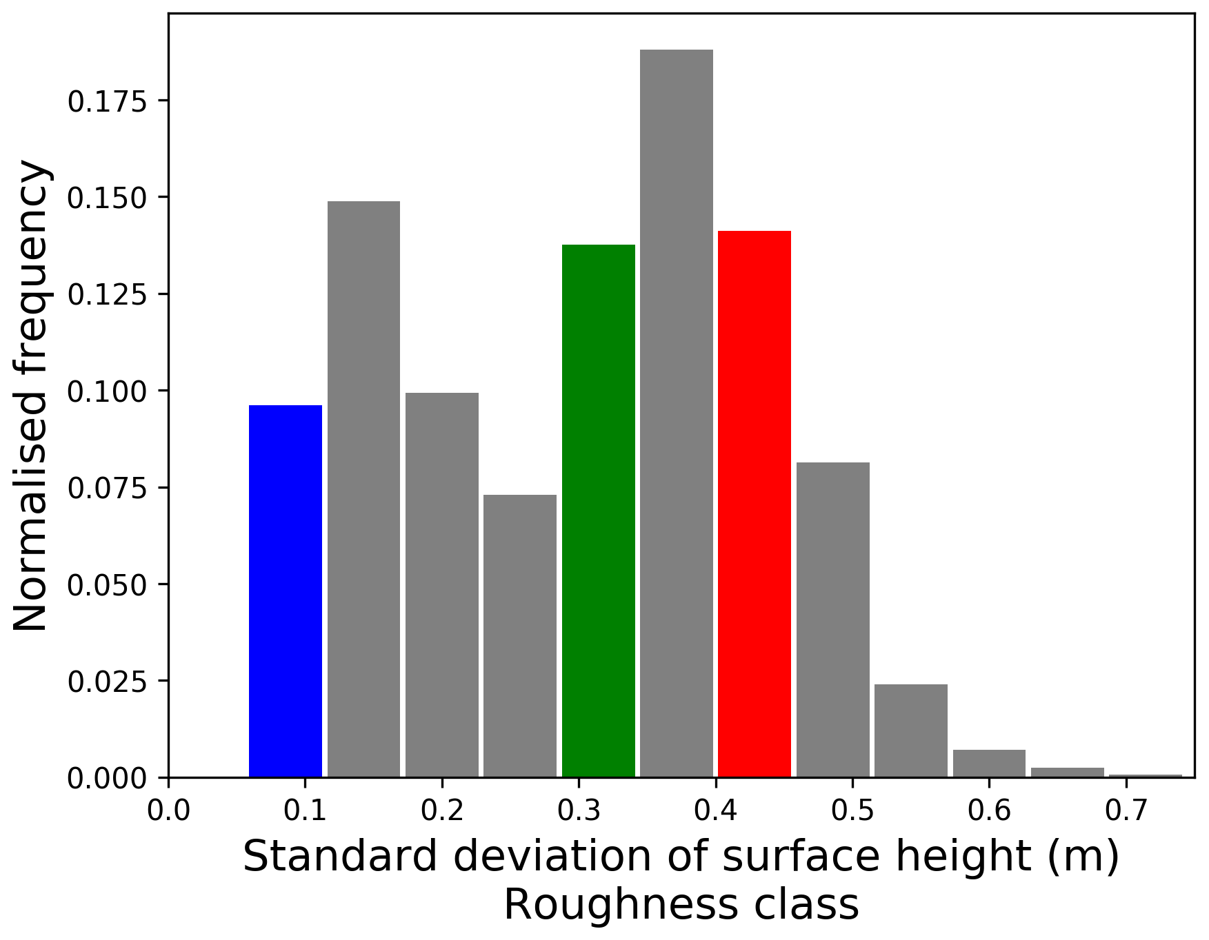
Figure 2Histogram of the standard deviation of surface heights computed from 70 m flight strips; bins define the roughness classes of sea ice. Examples for the three roughness classes “smooth”, “medium rough”, and “rough” are marked in the colours blue, green, and red, respectively.

Figure 3The fR parameter illustrating the deviation from the uniform azimuth distribution along 1000 randomly selected samples. The average value of fR is marked as a thick red line. The considered threshold of uniform distribution, 4.3 km, is marked by the blue dashed line.
In the second step, we interpolate the ALS elevation measurements to a regular 0.5 m grid in order to form a digital elevation model (DEM) of the sea ice surface. The sea ice surface in the DEM is represented as a set of triangular facets. Each facet orientation in the 3-D Cartesian space (for simplicity we assume the base vectors to be aligned with the aircraft principal axis, so points to the flight direction) is described by two angles: facet slope α () and facet azimuthal direction γ (). Therefore, the ith facet local normal vector is described by
In the third step, we compute the normal vectors and their orientations for the individual facets. This is done for all roughness classes. We found that the azimuthal orientation angle γ does not show any preferred directions within any given roughness class. In the next subsections we present the analysis of the two angles characterising the facet: azimuthal direction and surface slope.
2.2.1 Facet azimuth orientation
In the previous section we used the DEM to calculate the vectors normal to the surface facets. In this subsection we analyse the orientations of facet azimuths. In order to evaluate the distribution of the facet azimuths, we define parameter fR (Eq. 2). This parameter is calculated from a histogram of azimuth orientation. In Eq. (2) the denominator is the total number of measurements expressed as the number of angular bins multiplied by the mean number of samples per bin (total number of samples). The numerator is a sum of the differences between the mean number of samples per bin and the actual number of samples in each bin. There are 36 bins. The number of bins was determined with Nbins=5log 10(Ndata) considering the maximal number of samples in the 25 km flight track. The fR parameter equals zero for the perfectly uniform distribution, in which case the number of counts in each bin (ni) equals a mean number of counts (μ). The fR parameter reaches its maximum value of when the slopes are aligned, i.e. grouped in two bins.
To evaluate fR we selected 1000 random 15 km samples from the flight tracks. The analysis of the samples shows that the deviation from the uniform distribution decreases sharply with increasing distance over the first kilometre (Fig. 3). For distances along the flight track greater than 4.3 km the curve flattens at a value of fR=0.05 in 90 % of the samples. We assume that at scales greater than 4.3 km (marked by the vertical dashed line in Fig. 3) slope orientations do not have a preferential direction beyond natural variability. This distance corresponds to an approximately 60 s section. In Fig. 3 the average value of fR is marked as a thick red line. Several sample profiles are plotted as grey lines to illustrate the variability.
2.2.2 Facet slope angle
Section 2.2.1 looked at the azimuthal orientation of surface facets. This section focuses on the analysis of facet slopes. For all roughness classes we observe a similar probability density function (PDF) of surface slopes. The PDFs have a maximum at zero and a gradual decline in the likelihood of encountering the steeper slopes. Figure 4 shows the PDFα on a logarithmic scale for the three distinct roughness classes: smooth 0.05 m < σz < 0.11 m (in blue), medium rough 0.28 m < σz < 0.34 m (in green), and rough 0.45 m < σz < 0.51 m (in red).
We decide to approximate the PDF of surface slopes with an exponential curve:
where Cnorm is the normalisation constant and sα is the “geometrical-slope roughness parameter”. Figure 4 presents the data and the exponential approximations. The log scale is very relevant because it becomes obvious that the chances of encountering steep slopes are getting slimmer the higher the slope angle. Consequently, it makes sense that the approximation functions misfit the observations at high slope angles as it is irrelevant to fit an approximation there. As sα is the only parameter of the approximation function, it is descriptive of the surface roughness.
Figure 5 shows the relation between sα and the standard deviation of surface heights corresponding to the roughness classes defined above. The error bars represent the uncertainty associated with each data point. Very rough ice has a large uncertainty because the number of samples was small (classes with σz>0.6 m accounted for less than 75 s of flight, out of a total 78 min). The quadratic relation is holding well for ice with up to 0.5 m standard deviation of surface heights. The equation of the fitted curve is .
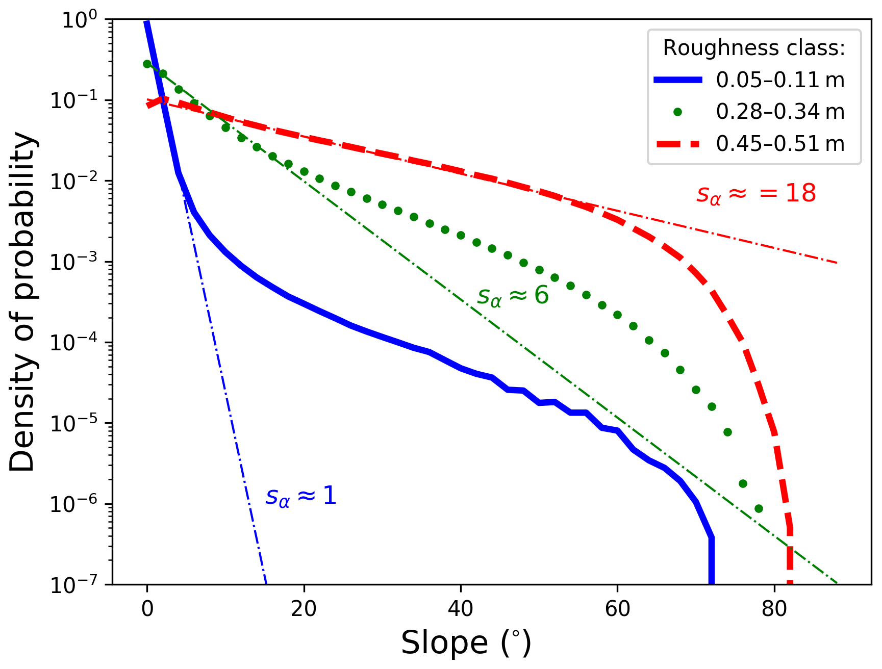
Figure 4Density of probability of surface slopes on a logarithmic scale for three roughness classes: smooth 0.05 m < σz < 0.11 m (in blue), medium rough 0.28 m < σz < 0.34 m (in green), and rough 0.45 m < σz < 0.51 m (in red). The exponential fits to the respective curves are marked as thin coloured dotted lines.

Figure 5Surface roughness parameter sα describing the probability distribution of surface slopes. Error bars are inversely proportional to the number of data points in each roughness class. The “smooth”, “medium rough”, and “rough” classes are marked in the colours blue, green, and red, respectively. The red dashed line marks the fitted curve.
2.3 Sea ice brightness temperature simulation
In this subsection we present the emission model for simulating the sea ice brightness temperature (TB). We use the MIcrowave L-band LAyered Sea ice emission model described by Maaß et al. (2013), further referred to as MILLAS. This model is based on the radiative transfer model of Burke et al. (1979) (who used it for soils), with infinite half-space of seawater covered with layers of sea ice, snow, and a top semi-infinite layer of air. In contrast to the original model of Burke et al. (1979) and its usage by Maaß et al. (2013), the current version of MILLAS takes into account multiple reflections at the layer boundaries. The multiple reflections are expressed as subsequent terms of a geometric series. The summation over series stops when terms of the series contribute less than a given threshold to the total (in the following calculations the threshold was set to 0.001). MILLAS describes the brightness temperature above snow-covered sea ice as a function of temperature and permittivity of the layers. The water permittivity depends mainly on the water temperature and salinity (Klein and Swift, 1977). Ice permittivity can be approximately described as a function of brine volume fraction (Vant et al., 1978), which depends on ice salinity and the densities of the ice and brine (Cox and Weeks, 1982), which in turn depends mainly on ice temperature. We set the ice salinity to 4 g kg−1 which is a mean value for first-year ice determined by Cox and Weeks (1974). The permittivity of dry snow can be estimated from its density and temperature (Tiuri et al., 1984). In the simulation, the ice and water salinity are kept constant (see Table 1). Furthermore, we assume that the system is in thermal equilibrium and that the water beneath the ice is at the freezing point. In this configuration, the TB is simulated as a function of ice thickness (dice), snow thickness (dsnow), and surface temperature (Tsurf). In our setup, the snow is assumed to be dry with a density of 300 kg m−3, which is the average snow density value for December Arctic measurements from 1954 to 1991 (Warren et al., 1999). The TB simulations are only slightly sensitive to snow density; see Fig. 3 in Maaß et al. (2013). The permittivities of snow and ice are linked to their temperature. The temperature profiles within snow and ice are assumed to be continuous and linear. The values for the ice and snow thermal conductivity are taken from Yu and Rothrock (1996) and Untersteiner (1961). As the optimisation of the emission model lies beyond the scope of this work, we use the simplest setup variant of MILLAS consisting of a single layer of ice covered with a single layer of snow.
Table 1Brightness temperature simulation setup of the MIcrowave L-band LAyered Sea ice emission model (MILLAS).

2.4 Simulation of brightness temperature of rough sea ice
In the previous sections, we described the sea ice surface as composed of facets with an orientation described by two angles: the slope α and the azimuthal direction γ. Subsequently, we analysed the ALS data to extract information about statistical distributions of slopes and their orientation. We concluded that the exponential function is suitable to describe the probability density function of surface slopes for a range of ice surfaces with different degrees of surface roughness.
In this section, we describe how we integrate the probability description of faceted sea ice surface with the MILLAS emission model. We will start by describing the coordinate system that we used in the TB simulations. The relations between radiometer antenna-look direction () and the horizontal () and vertical () polarisation vectors are described in a Cartesian coordinate system. We show how these relations are represented in the coordinate system associated with a facet. The vectors defined in the tilted facet coordinate system are denoted with the subscript i. Subsequently, we will derive the equation that sums up the emissions originating from multiple facets.
We consider the Cartesian coordinate system (, , ) with the origin in the centre of the nadir sensor footprint. In this reference frame the radiometer antenna-look direction () is described as
where the θ0 is the antenna incidence angle and the ϕ0 is the azimuthal direction of the antenna. In this particular case we set the reference system so ϕ0=0 and is parallel to the ground. The antenna setting defines the directions of the horizontal () and vertical () polarisation vectors:
We are interested in finding a relationship between the radiation originating from a tilted facet and from a flat one. For that purpose we must consider the tilted coordinate system associated with the ith facet (variables associated with individual facets are denoted with the subscript i). The z coordinate in this tilted coordinate system is aligned with the facet normal vector , followed by and calculated accordingly.
Therefore, the local incidence angle θi is
and the local horizontal and vertical polarisation vectors are
The emissions from the facet at an angle θi and polarisation p are denoted with an asterisk: . In order to calculate the brightness temperatures observed in the global horizontal and vertical polarisation, it is necessary to account for the coordinates' rotation (Ulaby et al., 2014, p. 443):
We model the sea ice surface as a set of facets. Therefore the brightness temperature registered at the antenna aperture is a sum of contributions from N facets. We assume that each facet area A at the distance R is visible at the incidence angle θi and covers a patch of antenna field of view, equal to the solid angle Ωi:
The formula summing the contributions from N visible facets is
with ωi the antenna gain component.
At this stage of our study, we aim at modelling the effect of surface roughness on the TB. As a first-order approximation we assume that the antenna gain is constant across the whole field of view and that the antenna is in a far field so the incidence angle θ0 is assumed constant across the field of view. This assumption is more suitable for the space-borne system. The resulting formula is
This is the formula that we implement in the geometrical roughness model. Figure 6 presents the data flow in the geometrical roughness model. The model merges the MILLAS emission model (suitable for sea ice) with the geometrical characterisation of the faceted surface. In the presented setup the MILLAS emission model uses the sea ice surface temperature (Tsurface), sea ice thickness (dice), and snow thickness (dsnow) as input variables. The GO part needs the cumulative probability distribution of surface slopes (CDFα) and the antenna look direction (). The orientation of N facets representing the sea ice surface is calculated with the inverse transform sampling (ITS) (Devroye, 2006). This method returns a random slope value from a given non-uniform distribution. The non-uniform distribution is described by a cumulative probability distribution, which in this case depends on the geometrical roughness parameter sα. Similarly, the azimuthal angle γi is drawn from a uniform distribution. The result of this processing step is the set of N pairs of angles (αi, γi) describing the orientation of N facets. In the next step, the local normal vector and the local incidence angle (θi) are calculated for each of the N facets. The θi is used to calculate the brightness temperature emitted from the ith facet with the emission model. Shadowing occurs when and the radiation is emitted away from the antenna. In the current setup the double-bounce effects are not accounted for. and are used to calculate the local and global polarisation directions, as well as Ωi. For the final step, the summed contributions from N facets are summed as in Eq. (12). The result is the brightness temperature of the surface observed under θ0 and polarisation p.
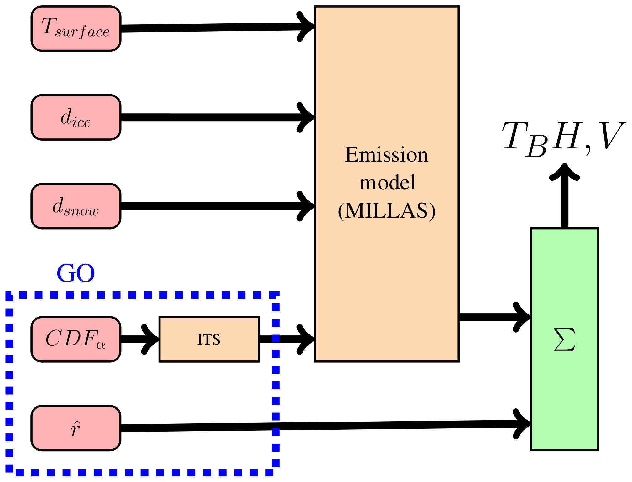
Figure 6Flow chart showing the processing chain within the geometrical roughness model. The model consists of two principal blocks: the emission model and the inverse transport sampling ITS module responsible for generating the facet orientation. The input parameters surface temperature Tsurface, ice thickness dice, snow thickness dsnow, cumulative distribution of surface slopes CDFα, and antenna direction are colour coded in red.
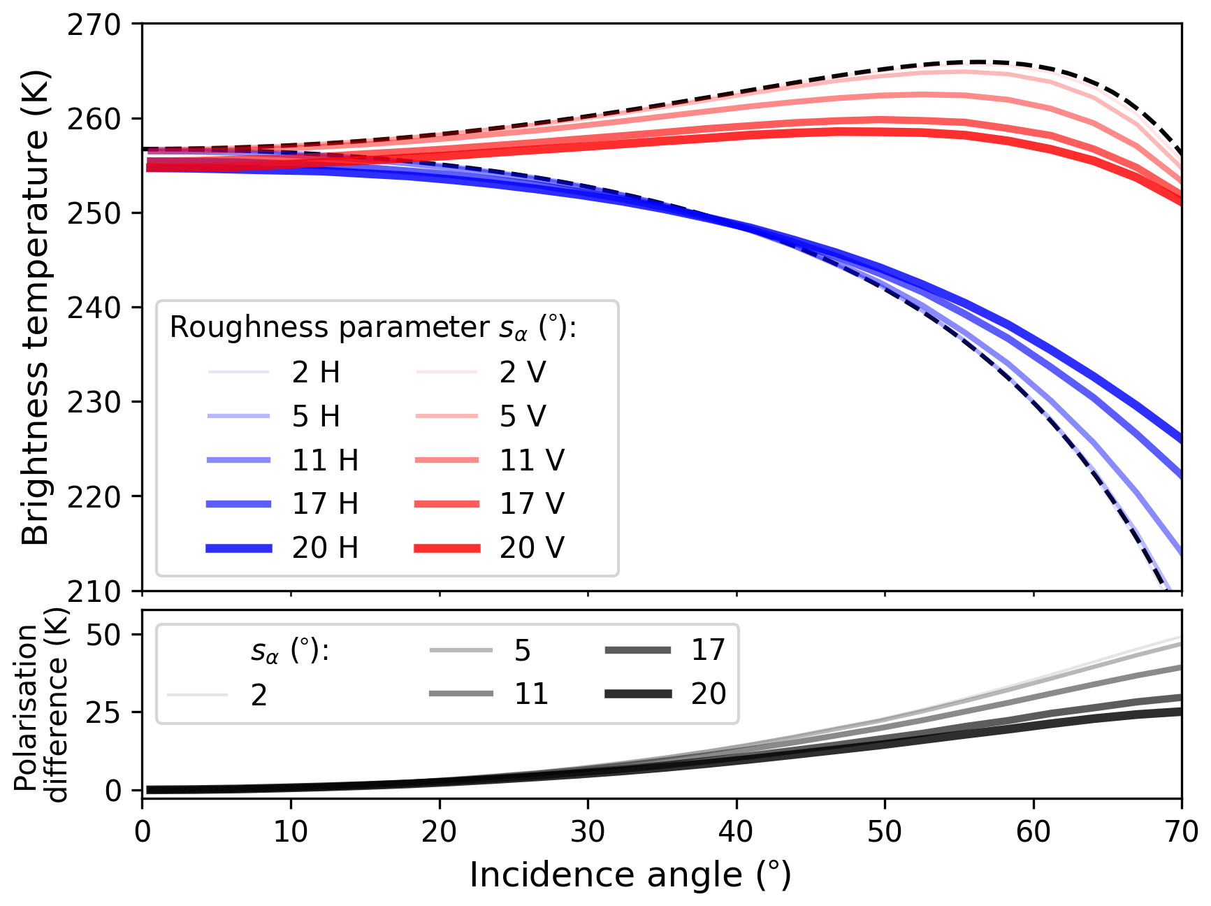
Figure 7Effects of the large-scale surface roughness on the brightness temperature of sea ice, simulated with the geometrical roughness model. Vertical polarisation is in red, and horizontal polarisation is in blue. The black dashed lines mark the TB for the specular surface. The surface roughness parameter sα varies between 2 and 20; the thicker the line the higher the sα. The inputs for the MILLAS emissivity model are kept constant: Tsurface=260 K, dice=1.42 m, and dsnow=0.14 m.
The number of facets N impacts the quality of the simulation and the reproducibility of the results. In order to set the value of N, we looked at the standard deviation of 20 TB simulation results for nadir and 45∘. We decided that the standard deviation of TB should be lower than 0.1 K, as this is the accuracy of the EMIRAD-2 radiometer for the 1 s integration time. This criterion is met for N greater than 104, which we take as the N value for further simulations.
The three main results of this study are as follows. (a) Surface roughness reduces the polarisation difference; this change is most pronounced at incidence angle greater than 50∘. (b) Nadir TB is little affected. (c) Comparison with the radiometer data and sensitivity study indicates that snow cover has a greater impact on the TB than surface roughness.
In Sect. 3.1 we show the brightness temperature simulations for sea ice with different degrees of large-scale surface roughness. To interpret the results we conduct a sensitivity analysis (Sect. 3.2). The comparison of the simulated vs. measured TB over 4.3 km flight track samples is shown in Sect. 3.3.
3.1 Brightness temperature simulations
In Sect. 2.2.2 we derived a parameterisation of the degree of surface roughness. We approximate the roughness by an exponential probability distribution function (PDF) of surface slopes. The shape of the PDF is fully described by the sα parameter.
In our simulation sα varies between 2 and 20 in accordance with the measurements of surface slopes conducted during SMOSice 2014. As the aim of this study is to characterise the effect of surface roughness on L-band TB, in this section we keep the other parameters of the emissivity model constant: surface temperature and ice and snow thickness (Tsurface=260 K, dice=1.42 m, dsnow=0.14 m). The brightness temperatures are calculated for every degree of incidence angle in the range 0–70∘. Figure 7 shows the simulation results.
The effect of increasing surface roughness is two-fold. First, the overall near-nadir intensity is lowered by 2.6 K. Second, the polarisation difference decreases. For the highest value of the roughness parameter, at Brewster's angle the vertical polarisation decreases by 8 K and horizontal polarisation experiences a 4 K increase. The effect of roughness is more pronounced for larger values of roughness parameter sα and is most visible at higher incidence angles (60∘).
The polarisation mixing can be explained by the approach used in this study. The emissions from the facet in horizontal () and vertical () polarisations are partially mixed when expressed in the () coordinate system (see Eq. 12).
The lowering of the intensity has two possible explanations. First is that our model does not take into account shadowing effects. When local incidence angle is greater than 90∘, the facet is emitting away from the antenna. For the “near-nadir” angles (0–30∘), the likelihood of shadowing is less than 1 % for the most rough ice (see Fig. 4).
The second explanation of this effect is associated with shape of the Fresnel emissivity curves. The polarisation difference for large incidence angles is larger than for the near-nadir ones. Therefore, the mean of the two polarisations ( i.e. total intensity) is fairly constant up to 30∘ and than drops continuously ∼ 10 K by 60∘. The trend continues for higher incidence angles. High values of sα increase the likelihood of returning a large incidence angle in the inverse transform sampling. These large incidence angles contribute to the overall lowering of the TB. The contribution of this mechanism is ≈ 2 K for TB(0) in the case of the most rough ice. The 2 K estimate was obtained by integrating the drop in total intensity weighted by the PDFα.
The above results are obtained with a Monte Carlo simulation. This method is a time-consuming approach. Therefore, we propose a parameterisation of the simulation results. The two effects, the polarisation mixing and the lowering of brightness temperature, can be expressed in a fashion similar to the HQ model proposed by Choudhury et al. (1979). Here we propose a formulation with two parameters Hα and Qα.
where p and q stand for the polarisation.
Hα accounts for the change in total intensity and Qα for the polarisation mixing. The emissions from the specular surface are denoted with an asterisk: . The proposed parameterisation approximates the results obtained with the Monte Carlo simulation with a root-mean-square difference of 0.45 K:
where , a0=1 and , b0=0.
The emissions from the specular surface are an essential input for the geometrical roughness model used in this study. The exact shape of the simulated brightness temperature curves depends on the probability distribution of slopes as well as on the emission characteristics of the specular surface. In this paragraph, we will investigate how the shape of the influences the geometrical roughness model results. The shapes of the polarisation curves, i.e. the reflectivities for a given incidence angle, are described by the Fresnel equations. Equations that are determined by the permittivity of the medium (ϵ). (In this section we omit the question of penetration depth assuming that the emissions are coming from the isothermal ice layer of constant permittivity.) To investigate the impact of the varying ϵ, we take a range of permittivities specific to sea ice as calculated within the MILLAS model. In the present setup the sea ice permittivity depends on bulk ice salinity and ice temperature. We calculate the ϵ for a range of ice temperatures (250 K < Tice < 271 K) and salinities (1 g kg−1 12 g kg−1).
The sea ice permittivities from the MILLAS model range between (for Tice=271 K, Sice=7 g kg−1) and (for Tice=253 K, Sice=1 g kg−1), where Tice is the bulk ice temperature and Sice is the bulk ice salinity. The curves corresponding to those values lie close together, indicating that the proposed parameterisation is suitable for all types of sea ice. The effect of permittivity on the polarisation mixing parameter (Qα) is less pronounced. The dependence of the Qα parameter on the roughness follows a similar quadratic curve regardless of the surface permittivity.
3.2 Sensitivity analysis
In this section, we investigate how sensitive the model is to its main variables: surface temperature, ice thickness, snow thickness, surface roughness, and the implicit assumption of 100 % sea ice concentration. This is a mandatory step toward the evaluation of the model (Sect. 3.3).
The two most important factors influencing the L-band brightness temperature over sea ice are the ice concentration and the ice thickness. We calculate the sensitivity of our model with regard to sea ice concentration by assuming a linear mixing of water and thick ice fractions within the radiometer footprint. The brightness temperature of seawater TBw (salinity of 33 g kg−1, temperature 271.2 K) is approximately 110 K, and of thick sea ice (Tsurf=260 K, dice=1.5 m, bulk salinity of 3 g kg−1) is 240 K. The resulting sensitivity to sea ice concentration is ≈ 1.5 K %−1.
The sensitivity of the TB to sea ice thickness over thin sea ice (dice<0.75 m) is fundamental for the sea ice thickness retrieval from L-band radiometry. TB saturates when the sea ice thickness is significantly larger than the penetration depth of the L-band radiation. Therefore, our analysis focuses on sea ice thicker than 1 m, in order to single out the contributions of surface roughness.
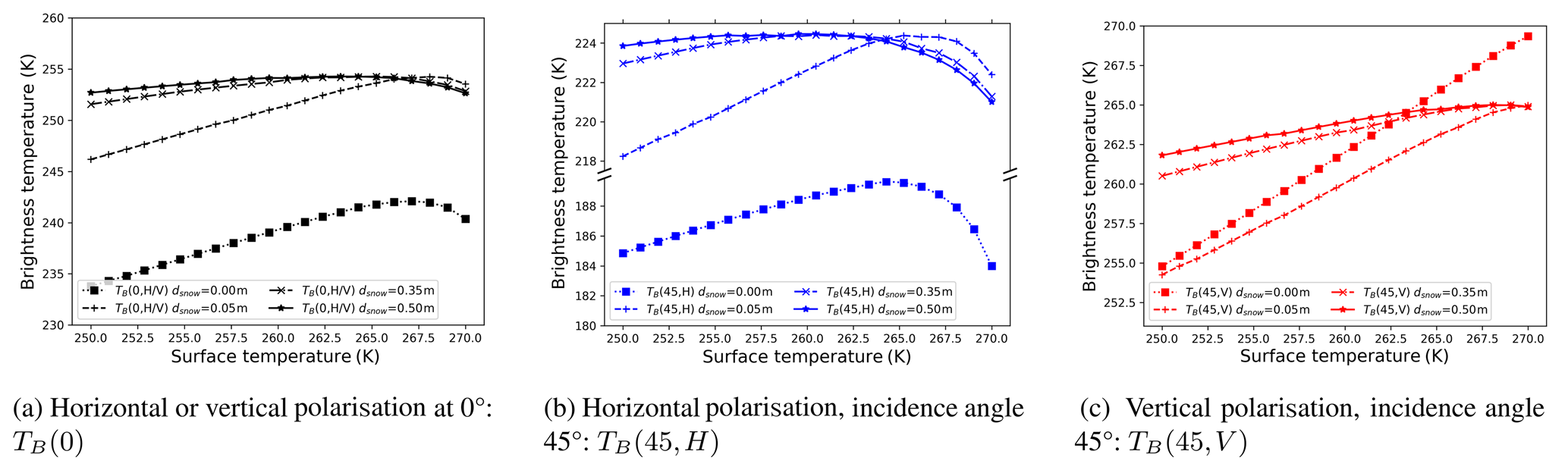
Figure 8Change in the brightness temperature as predicted by the MILLAS emission model as a function of surface temperature. The different line styles correspond to the different snow thickness assumptions. The calculation was carried out for the sea ice thickness of 1 m and surface roughness set to zero.
Table 2Table with sensitivities of the brightness temperature at nadir, 45, and 60∘ as simulated with geometrical optics surface roughness model. The input parameters are roughness parameter salpha, ice thickness dice, snow thickness dsnow, and surface temperature Tsurf.

Table 2 contains the sensitivities of the geometrical roughness model to the input parameters: roughness parameter sα, ice thickness dice, snow thickness dsnow, and surface temperature Tsurf. Presented values are grouped into columns corresponding to the polarisation and three incidence angles: 0, 45, and 60∘. The angles are chosen to reflect the antennae configuration during SMOSice 2014 with an addition of 60∘, close to Brewster's angle where surface roughness effects are most pronounced.
The assumption about snow thickness has a considerable effect on the sea ice TB (Maaß et al., 2013). For this reason the values of sensitivities are considered for a number of snow thickness values. Figure 8 shows the simulated L-band brightness temperatures at 0∘ and 45∘ as a function of the surface temperature. In this study we make considerable assumptions about snow thickness. To illustrate the uncertainty associated with the assumptions, the simulations are made for a range of snow thicknesses plotted in different line styles.
In the MILLAS model, ice permittivity is parameterised with ice temperature. The non-monotonic shape of the curves is caused by change in ice permittivity. Therefore, the sensitivities are calculated for two temperature ranges: lower (250–265 K) and higher (265–270 K). Table 2 contains the calculated sensitivities.
As far as the large-scale surface roughness is concerned, the sensitivity increases almost linearly for the values of sα between 0 and 20∘, which is the maximal value measured during the SMOSice 2014 campaign.
In order to interpret the results of the comparison between the simulation and measurements, it is necessary to evaluate the uncertainties associated with the input parameters: surface temperature, ice thickness, and snow thickness. In the following paragraphs, we use ”mean model sensitivity for the cold conditions” for the averaged absolute sensitivity of and at 250 K. We take the values for the lower temperature range as they match the conditions during the SMOSice 2014 campaign.
The uncertainty associated with surface temperature is estimated as the product of the sensitivity of the model times the measurement uncertainty. The surface temperature measurements carried out with the KT19.85 have an accuracy of 0.5 K. The mean surface temperature in the region covered by ice was 251.7 ± 3.5 K. We take the standard deviation of surface temperature measurements as the parameter uncertainty. We estimate the uncertainty associated with surface temperature to be 0.7 K.
The uncertainty associated with sea ice thickness is estimated as the product of the sensitivity of the model times the measurement uncertainty. The sea ice thickness measurements in this study are derived from the resampled ALS elevation data. The mean standard deviation of the resampled elevation measurements is 0.08 m. The assumption about the densities of snow, ice, and water combined with the assumption on the snow thickness of 1∕10 of ice thickness lead to the uncertainty of 0.4 m. Taking into account the mean model sensitivity for the cold conditions prevailing during the flights, we estimate that the uncertainty associated with sea ice thickness is 0.5 K.
The uncertainty associated with snow thickness is estimated as the product of the sensitivity of the model times the measurement uncertainty. Unfortunately, the snow thickness measurements are not available. The snow layer, although transparent for the L-band radiation, is not invisible. The refraction on the snow–ice and snow–air interfaces alters the local incidence angles. Snow cover also has an effect on the temperature profile within the ice. This indirectly affects the permittivity of sea ice. All these factors make an estimation of the uncertainty caused by snow thickness especially hard to quantify. We assume that snow thickness uncertainty is equal to the mean standard deviation of the resampled elevation measurements, that is 0.08 m. The mean model sensitivity to snow thickness for the cold conditions is 8.6 K m−1. Therefore, we estimate the uncertainty associated with snow thickness to be 0.7 K.
An important factor which is not directly included in the model is the sea ice concentration. In the model we assume sea ice concentration to be 100% in order to single out the much smaller contribution of surface roughness. However, if a linear mixing model is applied, the sensitivity to sea ice concentration is −1.5 K %−1. During the preprocessing of the airborne laser scanner (ALS) data we excluded the 70 m sections with more than 5 % missing values. The missing values are caused by the instrument setup (rotating mirror, edge of swath) or by the lack of return reflection from open water or thin ice. We estimate that the uncertainty associated with the sea ice concentration is up to 7.5 K.
To put the partial sensitivities into perspective, the expected changes in the TB caused by the strongest surface roughness measured during the SMOSice 2014 campaign do not exceed −2.2 K for nadir and 1 K and −5.6 K for the horizontal and vertical polarisation of the 45∘ antenna, respectively.
To conclude, the sensitivity analysis of the geometrical roughness model leads to the conclusion that the surface roughness effects will be hard to observe in the SMOSice 2014 flight data with the current emission model setup.

Figure 9Scatter plots illustrating the comparisons between the EMIRAD-2 data and the TB simulated without GO roughness included – specular. Results corresponding to the setup with snow are marked in green, and without snow is in blue.
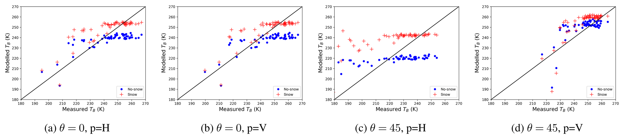
Figure 10Scatter plots illustrating the comparisons between the EMIRAD-2 data and the TB simulated with GO roughness included. Results corresponding to the setup with snow are marked in green, and without snow is in blue.
3.3 Simulations vs. measurements
In this section, we compare the brightness temperature measured with the EMIRAD-2 radiometer with the brightness temperature simulations. The comparison is done on a 4.3 km section as to justify the assumption of the isotropic azimuth distribution. We want to determine the simulation setup that best reproduces the radiometer measurements and whether the inclusion of the surface roughness in the simulation brings significant improvement. The limitation of this approach is that we assume that the ice observed by the side-looking antenna and the ice below the flight path have the same properties. We consider the surface temperature, the sea ice thickness, and the surface roughness along the flight, and we use them to run the statistical roughness model, described in Sect. 2.4 with the MILLAS single ice layer setup as the brightness temperature module. In setups including snow layer, the snow thickness is set to be 10 % of the sea ice thickness. The calculation is done for 60 s averages, during which the aircraft covers the distance of approximately 4.3 km. At this scale we consider the surface slopes' orientation to be isotropic. The measured surface slopes are used to compute empirical CDFα. Analysis at the 4.3 km scale is justified by the fact that the antennae gains are not known. Furthermore, the averaged sea ice properties are more representative for the space-borne radiometers.
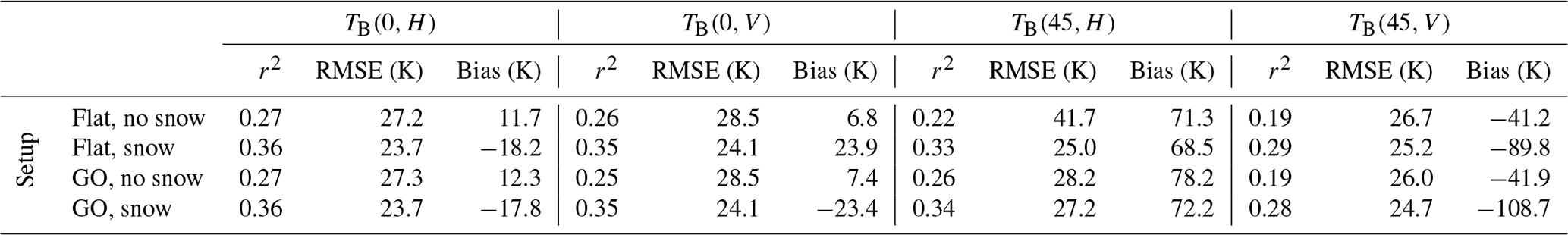
For each radiometer channel we made four simulation setups: two without roughness (Flat no snow, Flat snow), and two with roughness included (Rough (GO) no snow, Rough (GO) snow). As for the performance metrics of the model setups, we use the coefficient of determination (r2), the root-mean-square error (RMSE), and bias. These metrics are widely used in the assessment of the performance of satellite measurements (Entekhabi et al., 2010). Table 3 contains the results of the comparison expressed in terms of r2, RMSE, and bias. The corresponding scatter plots illustrating the comparison between measured and modelled brightness temperatures are presented in Figs. 9 and 10.
The values of r2 for all “channel–simulation setup” combinations do not exceed 0.36. The simplified one-layer model managed to capture only 36 % of the signal variance even with surface roughness included. Furthermore, the inclusion of surface roughness brings little improvement to the statistics. In the case of vertical polarisation, where the model studies indicate the most sensitivity to roughness, the r2 is even a little lower. The inclusion of a very crude snow thickness parameterisation is more successful in capturing the radiometer measurements' variability. All metrics show that the four model setups perform poorly in reproducing the EMIRAD-2 measurements.
The results of the comparison are also presented in the form of histograms of the difference between the measured and simulated TB (Fig. 11). For all four antenna feeds the RMSE between simulated and measured TB decreases whenever the setups include snow. However, the bias increases.
The high values of RMSE and bias show a general misfit of the model to the data. The sensitivity study of the model presented in Sect. 3.2 indicates that the effects of surface roughness are of comparable magnitude or smaller than uncertainties associated with the model input parameters. The side-looking vertical polarisation is predicted to be most affected by the surface roughness. However, the surface roughness is not measured directly in the side-looking antenna footprint. The scatter plots in Figs. 9 and 10 and the calculated statistics show that a simplified one-layer model struggles to capture the dynamics of the sea ice TB regardless of the simulation setup.
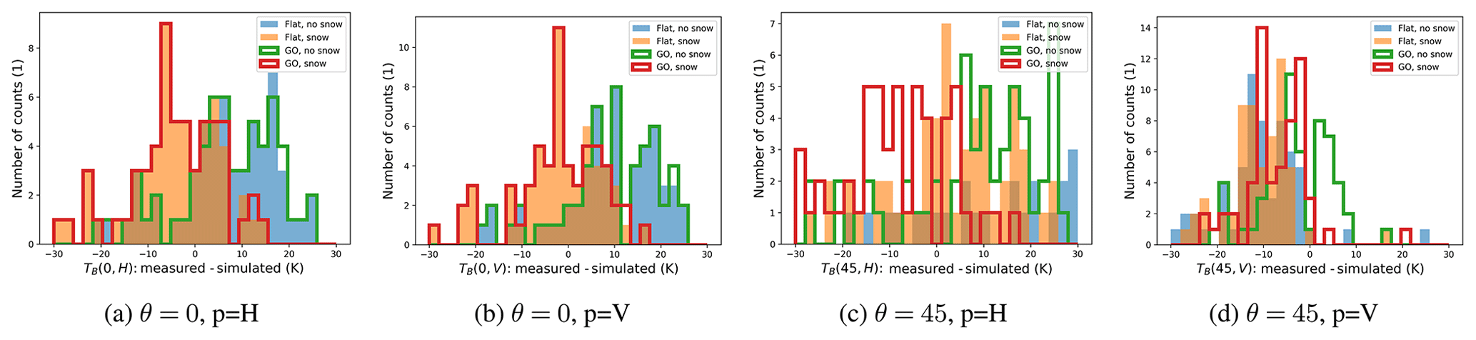
Figure 11Histograms of the differences between the EMIARAD2 measurements and simulation setups for four antenna feeds.
Table 3Performance metrics for the different TB simulation setups in terms of coefficient of determination r2, RMSE (K), and bias (K). For EMIRAD-2 channels four model setups are tested: Flat no snow, Flat snow, GO no snow, and GO snow.
In this paper we address the knowledge gap concerning the influence of the decimetre-scale surface roughness on the L-band brightness temperature of sea ice. We used the airborne laser scanner (ALS) data to characterise the sea ice surface and to produce the digital elevation model (DEM) of the sea ice surface. From the DEM we derived the probability distribution of surface slopes (α) and their azimuthal orientation (γ). We found that the probability distribution function of α (PDFα) can be described with an exponential function regardless of the degree of roughness of sea ice surface. The exponent parameter (sα) is a quasi-quadratic function of the standard deviation of surface heights. In the second part of this work, we used the PDFα in a Monte Carlo simulation of the emission from a faceted sea ice surface. The effect of surface roughness is marginal near the nadir, accounting for up to 2.6 K decreases in TB. The polarisation curves around Brewster's angle are most affected. The vertical polarisation decreases by 8 K, and horizontal polarisation increases by 4 K for the roughest ice, compared with the specular sea ice surface. The effect of the large-scale surface roughness on polarisation curves is not linear, with the degree of the surface roughness described by sα, meaning that the alteration of the TB curves is strongest for the roughest surface. The overall change of emission due to the large-scale surface roughness can be expressed as a superposition of change in intensity (Hα) and an increase in polarisation mixing (Qα). The change in intensity depends primarily on the surface permittivity, whereas the polarisation mixing shows little dependence on ϵ. This parameterisation is suitable for all types of sea ice. However, the sensitivity analysis of the simplified emission model demonstrates that the expected change in TB is comparable in magnitude to the uncertainty associated with the model input parameters.
The results have implications for the current and future L-band missions. The operational SMOS sea ice thickness product relies on near-nadir TB observations (0–30∘). Therefore, the large-scale surface roughness will have little effect on the retrieval. The SMAP and CIMR missions, which operate at incidence angles of 40 and 55∘, respectively, are more exposed to the surface roughness effects. The effect on the vertical polarisation is stronger than on the horizontal polarisation. Lastly, we compared the simulation of the brightness temperature (with and without surface roughness) with the radiometer measurements. Unfortunately, this showed that our model does not capture the brightness temperature variability at the scale of 4.3 km. The inclusion of surface roughness is less important than the inclusion of a crude snow thickness parameterisation. This is confirmed by the sensitivity analysis of the model. Another possible explanation is that the sea ice in the studied region was highly heterogeneous in terms of its thickness and snow cover. Furthermore, a simple two-layer emission model used in this study has its limitations in capturing the TB variability. Better results might be obtained if a multi-layer model together with the snow thickness measurements is used. With such a setup the direct inclusion of sea ice facets orientation in the radiometer field of view will be a valuable option to improve the TB simulation. However, this would require in situ measurements of sea ice permittivity, snow thickness, temperature, and roughness as well as detailed characterisation of the antenna gain. Thus, the authors' recommendation for future studies is to measure the microphysical snow and sea ice properties together with surface roughness directly in the radiometer's field of view.
| ALS | airborne laser scanner |
| CDF | cumulative distribution function |
| DEM | digital elevation model |
| GO | geometrical optics |
| ITS | inverse transform sampling |
| MILLAS | MIcrowave L-band LAyered Sea ice emission model |
| probability distribution function | |
| RFI | radio frequency interference |
| SAR | synthetic aperture radar |
| SMAP | soil moisture active and passive mission |
| SMOS | soil moisture and ocean salinity mission |
| TB | brightness temperature |
Code and data are available from the authors on request.
LK was the project PI responsible for funding acquisition, project administration, and supervision. Conceptualisation of the work presented in this paper was done by MM and LK. The problem investigation and methodology was done by MM, and the software implementation was carried out by MM and NM. The data curation was done by SH and SSS. As far as the writing and manuscript preparation are concerned, MM prepared the draft and the data visualisation with LK and NM doing the first reviews and editing.
The authors declare that they have no conflict of interest.
The authors acknowledge the institutions providing the data and people involved in carrying out the measurements. The TerraSAR-X and TanDEM-X teams provided the SAR data for this study.
Special thanks are due to Yann Karr, PI of the SMOS mission, for his suggestions and comments. We are also grateful for the financial support that covered the publication costs.
This research was funded by the HGF Alliance, Remote Sensing and Earth System Dynamics. The European Space Agency co-financed the AWI research aircraft Polar 5 and helicopter flights (ESA contract 4000110477/14/NL/FF/lf; PI Stefan Hendricks) and the development and validation of SMOS sea ice thickness retrieval methods (ESA contracts 4000101476/10/NL/CT and 4000112022/14/I-AM; PI Lars Kaleschke). Technical University of Denmark (DTU) co-financed and conducted the measurements with the EMIRAD2 L-band radiometer on Polar 5.
This paper was edited by John Yackel and reviewed by Jack Landy and Georg Heygster.
Balling, J. E., Søbjaerg, S. S., Kristensen, S. S., and Skou, N.: RFI detected by kurtosis and polarimetry: Performance comparison based on airborne campaign data, in: 2012 12th Specialist Meeting on Microwave Radiometry and Remote Sensing of the Environment, MicroRad 2012 – Proceedings, Rome, Italy, 5–9 March 2012, https://doi.org/10.1109/MicroRad.2012.6185255, 2012. a
Beckers, J. F., Renner, A. H. H., Spreen, G., Gerland, S., and Haas, C.: Sea-ice surface roughness estimates from airborne laser scanner and laser altimeter observations in Fram Strait and north of Svalbard, Ann. Glaciol., 56, 235–244, https://doi.org/10.3189/2015AoG69A717, 2015. a
Burke, W. J., Schmugge, T., and Paris, J. F.: Comparison Of 2.8- and 21-cm Microwave Radiometer Observations Over Soils With Emission Model Calculations, J. Geophys. Res., 84, 287–294, https://doi.org/10.1029/JC084iC01p00287, 1979. a, b
Choudhury, B. J., Schmugge, T. J., Chang, A., and Newton, R. W.: Effect Of Surface Roughness On The Microwave Emission From Soils, J. Geophys. Res., 84, 5699–5706, https://doi.org/10.1029/JC084iC09p05699, 1979. a
Cox, G. F. and Weeks, W. F.: Salinity variations in sea ice, J. Glaciol., 13, 109–120, 1974. a
Cox, G. F. N. and Weeks, W. F.: Equations For Determining The Gas And Brine Volumes In Sea Ice Samples, CRREL Report, US Army Cold Regions Research and Engineering Laboratory, 1982. a
Devroye, L.: Chapter 4 Nonuniform Random Variate Generation, in: Simulation, edited by: Henderson, S. G. and Nelson, B. L., Handbooks in Operations Research and Management Science, vol. 13 Elsevier, 83–121, https://doi.org/10.1016/S0927-0507(06)13004-2, 2006. a
Dierking, W.: Laser profiling of the ice surface topography during the Winter Weddel Gyre Study 1992, J. Geophys. Res., 100, 4807–4820, 1995. a
Dierking, W.: RMS slope of exponentially correlated surface roughness for radar applications, IEEE T. Geosci. Remote Sens., 38, 1451–1454, https://doi.org/10.1109/36.843040, 2000. a
Entekhabi, D., Reichle, H. R., Koster, D. R., and Crow, T. W.: Performance metrics for soil moisture retrievals and application requirements, J. Hydrometeorol., 11, 832–840, https://doi.org/10.1175/2010JHM1223.1, 2010. a
Hendricks, S., Steinhage, D., Helm, V., Birnbaum, G., Skou, N., Kristensen, S. S., Søbjærg, S. S., Gerland, S., Spreen, G., Bratrein, M., King, J., and Kaleschke,L.: SMOSice 2014: Data acquisition report, Technical support for the 2014 SMOSice campaign in SE Svalbard, ESA contract number: 4000110477/14/NL/FF/lf, available at: https://earth.esa.int/documents/10174/134665/SMOSice_2014_report (last access: 30 January 2020), 2014. a, b, c, d, e
Huntemann, M., Heygster, G., Kaleschke, L., Krumpen, T., Mäkynen, M., and Drusch, M.: Empirical sea ice thickness retrieval during the freeze-up period from SMOS high incident angle observations, The Cryosphere, 8, 439–451, https://doi.org/10.5194/tc-8-439-2014, 2014. a
Kaleschke, L., Tian-Kunze, X., Maaß, N., Beitsch, A., Wernecke, A., Miernecki, M., Müller, G., Fock, B. H., Gierisch, A. M. U., Schlünzen, K. H., Pohlmann, T., Dobrynin, M., Hendricks, S., Asseng, J., Gerdes, R., Jochmann, P., Reimer, N., Holfort, J., Melsheimer, C., Heygster, G., Spreen, G., Gerland, S., King, J., Skou, N., Søbjærg, S. S., Haas, C., Richter, F., and Casal, T.: SMOS sea ice product: Operational application and validation in the Barents Sea marginal ice zone, Remote Sens. Environ., 180, 264–273, https://doi.org/10.1016/j.rse.2016.03.009, 2016. a, b, c
Ketchum, R.: Airborne laser profiling of the arctic pack ice, Remote Sens. Environ., 2, 41–52, 1971. a
Klein, L. and Swift, C.: An improved model for the dielectric constant of sea water at microwave frequencies, IEEE T. Antenn. Propag., 25, 104–111, https://doi.org/10.1109/TAP.1977.1141539, 1977. a
Landy, J., Isleifson, D., Komarov, A., and Barber, D.: Parameterization of Centimeter-Scale Sea Ice Surface Roughness Using Terrestrial LiDAR, IEEE T. Geosci. Remote,, 53, 1271–1286, https://doi.org/10.1109/TGRS.2014.2336833, 2015. a, b
Lawrence, H., Demontoux, F., Wigneron, J. P., Paillou, P., Wu, T. D., and Kerr, Y. H.: Evaluation of a Numerical Modeling Approach Based on the Finite-Element Method for Calculating the Rough Surface Scattering and Emission of a Soil Layer, IEEE Geosci. Remote Sens. Lett., 8, 953–957, https://doi.org/10.1109/LGRS.2011.2131633, 2011. a
Lawrence, H., Wigneron, J., Demontoux, F., Mialon, A., and Kerr, Y. H.: Evaluating the semiempirical H-Q model used to calculate the L-band emissivity of a rough bare soil, IEEE T. Geosci. Remote, 51, 4075–4084, https://doi.org/10.1109/TGRS.2012.2226995, 2013. a
Liu, C., Chao, J., Gu, W., Li, L., and Xu, Y.: On the surface roughness characteristics of the land fast sea-ice in the Bohai Sea, Acta Oceanol. Sin., 33, 97–106, https://doi.org/10.1007/s13131-014-0509-3, 2014. a
Maaß, N., Kaleschke, L., Tian-Kunze, X., and Drusch, M.: Snow thickness retrieval over thick Arctic sea ice using SMOS satellite data, The Cryosphere, 7, 1971–1989, https://doi.org/10.5194/tc-7-1971-2013, 2013. a, b, c, d, e, f
Mäkynen, M., Cheng, B., and Similä, M.: On the accuracy of thin-ice thickness retrieval using MODIS thermal imagery over Arctic first-year ice, Ann. Glaciol., 54, 87–96, https://doi.org/10.3189/2013AoG62A166, 2013. a
Matzler, C. and Standley, A.: Relief effects for passive microwave remote sensing, Int. J. Remote Sens., 21, 2403–2412, https://doi.org/10.1080/01431160050030538, 2000. a
Panofsky, H. A. and Brier, G. W.: Some applications of statistics to meteorology, Pennsylvania State University Press, 1958. a
Prigent, C. and Abba, P.: Sea surface equivalent brightness temperature at millimeter wavelengths, Annales Geophys., 8, 627–634, 1990. a
Ricker, R., Hendricks, S., Helm, V., Skourup, H., and Davidson, M.: Sensitivity of CryoSat-2 Arctic sea-ice freeboard and thickness on radar-waveform interpretation, The Cryosphere, 8, 1607–1622, https://doi.org/10.5194/tc-8-1607-2014, 2014. a
Søbjaerg, S., Kristensen, S., Balling, J., and Skou, N.: The airborne EMIRAD L-band radiometer system, Melbourne, VIC, Australia, 21–26 July 2013, https://doi.org/10.1109/IGARSS.2013.6723175, 2013. a
Stroeve, J. C., Markus, T., Maslanik, J. A., Cavalieri, D. J., Gasiewski, A. J., Heinrichs, J. F., Holmgren, J., Perovich, D. K., and Sturm, M.: Impact of surface roughness on AMSR-E sea ice products, IEEE T. Geosci. Remote, 44, 3103–3116, https://doi.org/10.1109/TGRS.2006.880619, 2006. a
Strübing, K. and Schwarz, J.: Die Eisverhältnisse in der Barentssee während der IRO-2-Testfahrt mit R/V Lance 17.–27.03.2014, Tech. rep., 2014. a
Tian-Kunze, X., Kaleschke, L., Maaß, N., Mäkynen, M., Serra, N., Drusch, M., and Krumpen, T.: SMOS-derived thin sea ice thickness: algorithm baseline, product specifications and initial verification, The Cryosphere, 8, 997–1018, https://doi.org/10.5194/tc-8-997-2014, 2014. a
Tiuri, M. E., Sihvola, A. H., Nyfors, E. G., and Hallikaiken, M. T.: The Complex Dielectric Constant of Snow at Microwave Frequencies, IEEE J. Oceanic Eng., 9, 377–382, https://doi.org/10.1109/JOE.1984.1145645, 1984. a
Ulaby, F. T., Long, D. G., Blackwell, W. J., Elachi, C., Fung, A. K., Ruf, C., Sarabandi, K., Zebker, H. A., and Van Zyl, J.: Microwave radar and radiometric remote sensing, University of Michigan Press Ann Arbor, 2014. a, b, c, d, e
Untersteiner, N.: On the mass and heat budget of arctic sea ice, Archiv für Meteorologie, Geophysik und Bioklimatologie Serie A, 12, 151–182, 1961. a
Vant, M. R., Ramseier, R. O., and Makios, V.: The complex-dielectric constant of sea ice at frequencies in the range 0.1-40 GHz, J. Appl. Phys., 49, 1264–1280, 1978. a
Warren, S. G., Rigor, I. G., Untersteiner, N., Radionov, V. F., Bryazgin, N. N., Aleksandrov, Y. I., and Colony, R.: Snow depth on Arctic sea ice, J. Climate, 12, 1814–1829, https://doi.org/10.1175/1520-0442(1999)012<1814:SDOASI>2.0.CO;2, 1999. a, b
Yu, Y. and Rothrock, D. A.: Thin ice thickness from satellite thermal imagery, J. Geophys. Res.-Oceans, 101, 25753–25766, https://doi.org/10.1029/96JC02242, 1996. a, b