the Creative Commons Attribution 4.0 License.
the Creative Commons Attribution 4.0 License.
 | 14 Jan 2020
Modeling the evolution of the structural anisotropy of snow
Henning Löwe
Martin Proksch
Anna Kontu
The structural anisotropy of snow characterizes the spatially anisotropic distribution of the ice and air microstructure and is a key parameter for improving parameterizations of physical properties. To enable the use of the anisotropy in snowpack models as an internal variable, we propose a simple model based on a rate equation for the temporal evolution. The model is validated with a comprehensive set of anisotropy profiles and time series from X-ray microtomography (CT) and radar measurements. The model includes two effects, namely temperature gradient metamorphism and settling, and can be forced by any snowpack model that predicts temperature and density. First, we use CT time series from lab experiments to validate the proposed effect of temperature gradient metamorphism. Next, we use SNOWPACK simulations to calibrate the model with radar time series from the NoSREx campaigns in Sodankylä, Finland. Finally we compare the simulated anisotropy profiles against field-measured full-depth CT profiles. Our results confirm that the creation of vertical structures is mainly controlled by the vertical water vapor flux through the snow volume. Our results further indicate a yet undocumented effect of snow settling on the creation of horizontal structures. Overall the model is able to reproduce the characteristic anisotropy variations in radar time series of four different winter seasons with a very limited set of calibration parameters.
- Article
(11058 KB) -
Supplement
(10156 KB) - BibTeX
- EndNote


Deposited snow is a porous material that continuously undergoes microstructural changes in response to the external, thermodynamic forcing imposed by the atmosphere and the underlying soil. In some cases, the microstructure can develop a significant structural anisotropy; i.e., the nonspherical ice particles develop a preferential orientation, often in the vertical or horizontal direction. Among other microstructural properties, a significant amount of work was recently dedicated to understanding the impact of the structural anisotropy, which is a key parameter to improve predictions of different snow properties like the thermal conductivity (Izumi and Huzioka, 1975; Calonne et al., 2011; Shertzer and Adams, 2011; Riche and Schneebeli, 2013; Calonne et al., 2014), mechanical (Srivastava et al., 2010, 2016; Wiese and Schneebeli, 2017), diffusive, and permeable properties (Zermatten et al., 2011; Calonne et al., 2012, 2014), and the electromagnetic permittivity (Leinss et al., 2016, and references therein). In particular the thermal conductivity shows a strong dependence on the structural anisotropy (Löwe et al., 2013; Calonne et al., 2014). Depending on snow type, the thermal conductivity can vary by an order of magnitude at a given density: this variability is discussed with respect to the theoretical limits defined by a microstructure of either vertical or horizontal series of ice plates (Sturm et al., 1997).
The structural anisotropy is commonly characterized by different variants of geometrical or structural fabric tensors. These can be computed from mean intercept lengths (Srivastava et al., 2016), contact orientations (Shertzer and Adams, 2011), surface normals (Riche et al., 2013), or other second-order orientation tensors that can be constructed from the two-point correlation function of a two-phase medium (Torquato and Lado, 1991; Torquato, 2002). The correlation functions can be evaluated in terms of directional correlation lengths which define characteristic length scales of the microstructure (e.g., Vallese and Kong, 1981; Mätzler, 1997; Löwe et al., 2013) and from which the anisotropy can be derived. For snow, the microstructure can be obtained by stereology (e.g., Alley, 1987; Mätzler, 2002) or from computer tomography, CT (Schneebeli and Sokratov, 2004).
However the inclusion of the structural anisotropy in current snowpack models is still missing due to (i) the lack of a prognostic model for the anisotropy evolution and (ii) the lack of in situ data for validation. Motivated by recent progress of anisotropy measurements using radar (Leinss et al., 2016) as a solution for (ii) it is the aim of the present paper to overcome (i) and to suggest a minimal, dynamical model tailored to direct use in common operational snowpack models.
The model is based on a simple rate equation which incorporates temperature gradient metamorphism and snow settling. Each contribution is formulated in terms of common macroscopic state variables (temperature, temperature gradient, and strain rate) which are provided by detailed snowpack models like SNOWPACK (Bartelt and Lehning, 2002; Lehning et al., 2002a, b), CROCUS (Brun et al., 1989, 1992), or SNTHERM (Jordan, 1991). The magnitude of each contribution is controlled by free parameters which we calibrated with laboratory CT data and radar time series from Finland from which the anisotropy evolution over four winter seasons between October 2009 and May 2013 was obtained with 4 h resolution. The model links temporally high-resolution but vertically averaged anisotropy time series from radar with vertically high-resolution but temporally sparse CT measurements and is validated against field-measured, full-depth CT anisotropy profiles.
The paper is structured as follows: Sect. 2 discusses relevant processes which influence the structural anisotropy and casts them into rate equations. Section 3 presents experimental data and their integration for model forcing, calibration, and validation. Section 4 validates the influence of temperature gradient metamorphism (TGM) on the modeled anisotropy, presents the seasonal evolution of the anisotropy according to the full model, and validates these results with field-measured CT profiles. Section 5 discusses capabilities and deficits of the model and of anisotropy measurements. Section 6 concludes the paper, and the data availability section lists where to find the data. The Appendix details the preprocessing of meteorological data and the calibration of SNOWPACK.
The Supplement provides additional figures about the processing work flow, meteorological data and radiation balance, correlation lengths derived from CT data, an analysis of SNOWPACK ensemble members, visualizations of snow properties, and results of anisotropy model variants.
2.1 Definition of the anisotropy
For quantifying the structural anisotropy, we follow the definition in Leinss et al. (2016) and use the normalized difference of a characteristic horizontal length scale ax and a vertical length scale az:
Different characteristic length scales can be chosen. Commonly exponential correlation lengths are used as defined in Mätzler (2002). According to Eq. (1), the structural anisotropy ranges from −2 (vertical needles) to +2 (horizontal planes) with A=0 for randomly shaped or spherical particles (Fig. 1).
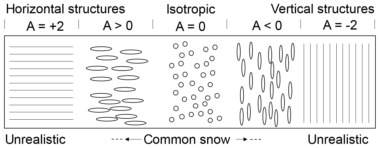
Figure 1Different structures and their anisotropy according to Eq. (1). Snow shows only a small anisotropy and can never reach the extreme cases of horizontal planes or vertical needles.
As detailed in Leinss et al. (2016), a normalized difference is convenient compared to the definition via an aspect ratio () because equally prolate and oblate particles with interchanged semiaxes then have the same magnitude for the anisotropy, and averaging them results in isotropy (A=0). The normalized difference and the frequently used grain size aspect ratio A′ are however equivalent and can be related by
This relation is helpful for a comparison with literature values. For snow a common range is but larger values might occur (Alley, 1987; Davis and Dozier, 1989; Schneebeli and Sokratov, 2004; Fujita et al., 2009; Calonne et al., 2014). In this range, equal to , the approximation in Eq. (2) deviates less then 5 % from A′ with respect to A′.
For conciseness, we refer to “horizontal structures” when the horizontal length scales are larger then the vertical ones, ax, ay>az; hence A>0. Accordingly, “vertical structures” describe snow with vertical length scales larger than horizontal ones, az>ax, ay, equivalent to A<0.
2.2 Evolution of the anisotropy
Quite generally, the anisotropy evolves from horizontal structures in new snow, over isotropic structures in decomposing rounded grains, to vertical structures under the influence of temperature gradient metamorphism (Schneebeli and Sokratov, 2004; Calonne et al., 2014) and might return to isotropy during melt processes. To describe this evolution we assume the following rate equation:
The first term accounts for the growth of vertical structures due to temperature gradient metamorphism (TGM), the most common type of snow metamorphism. The second term accounts for the formation of horizontal structures due to microscopic grain rearrangement causing the settling (strain) of snow. Further terms could be added to account for a possible rounding of grains by melt metamorphism. For simplicity we start with the assumption of an additive decomposition of these processes; though naturally, all these processes are coupled (e.g. Wiese and Schneebeli, 2017).
Since snow models commonly focus on the evolution of microstructural properties in individual snow layers (Bartelt and Lehning, 2002), we describe the anisotropy evolution in each layer with a Lagrangian viewpoint where the reference frame is attached to a material element. Therefore, we drop the z dependence in Eq. (3). Further, we restrict our model to flat terrain and do not consider any forces acting parallel to the snow layers (in the x or y direction). This implies that gravity and temperature gradient are strictly applied in the z direction.
2.3 Temperature gradient metamorphism
During TGM, ice crystals preferably grow into the opposite direction of the heat and water vapor flux, irrespective of whether the heat flux is applied in the horizontal or vertical direction (Yosida, 1955, pp. 52–56). The underlying water transport mechanism, mediated by a vapor flux from ice grain to ice grain, is often termed “hand-to-hand” transport as suggested by Yosida (1955, pp. 31–34). Pinzer et al. (2012) confirmed this mechanism and demonstrated a rapid reorganization of the ice matrix within a few days. The rapid reorganization renders the perception of a slowly growing ice grain misleading as “only the `memory' of the grain, encoded in the temporal correlation of the structure, survives” (Pinzer et al., 2012). Thereby, large vertical structures have a higher chance to survive while small structures quickly disappear.
To mimic this structural reorganization, we model the growth of vertical structures proportional to the magnitude of the water vapor mass flux: . We use the absolute value because the anisotropy does not contain any information about the growth direction but only about the growth orientation.
In winter, the vapor flux direction is usually positive (upwards) but can be reversed in spring, when the eventually melting snow surface is warmer than the underlying snowpack. With strong diurnal cycles, the flux direction can also alternate on a daily basis, but apparently these oscillating temperature gradients seem not to cause growth of faceted crystals: according to Pinzer and Schneebeli (2009) the morphology of the snow structure evolves slower and “did not show any sign of conventional TGM”. Therefore, we exclude the effect of daily alternating temperature gradients by averaging temperature gradients over 24 h:
As indicated in Fig. 1, perfect needle microstructures do not exist in reality. Therefore, we assume a minimal anisotropy Amin that can be practically attained by adding an empirical, quadratic weighting function. This function also amplifies the decay of horizontal structures modeled for new snow which should transform faster because small grains evaporate relatively quickly. The function also slows down the evolution of vertical structures which are modeled for snow which has experienced already strong TGM and has therefore relatively large grains. With these considerations, we model the growth of vertical structures by
The positive prefactor α1 defines the coupling strength of the right-hand side to the anisotropy change rate and must be determined from experiments. It has units of square meters per kilogram.
The vapor flux is mediated by diffusion, which is driven by a water vapor pressure gradient induced by a temperature gradient. Therefore, the vertical water vapor mass flux Jv () follows from Fick's law applied to the water vapor mass density ρv(T) (kg m−3):
The vapor mass density ρv is given by the water vapor pressure, pS(T), which is supposed to be at the saturation point in the pores between the ice crystals. Density and saturation pressure are related by the equation for ideal gases,
where is the specific gas constant for water vapor, the molar mass of water, and the universal gas constant. The saturation pressure over ice can be well approximated using different formulas (Marti and Mauersberger, 1993) and is given in Bartelt and Lehning (2002) by
with the latent heat of ice sublimation and the triple-point pressure and temperature of water, p0S=611.73 Pa and T0=273.16 K.
Because the saturation pressure, Eq. (8), depends only on temperature, Eq. (6) can be written in terms of temperature T and temperature gradient (Lehning et al., 2002b):
The effective diffusion constant for water vapor in snow, Dvs, is close to the diffusion constant in air, (Massman, 1998), and ranges between 1 and (Sokratov and Maeno, 2000; Colbeck, 1993) and is reviewed in Pinzer et al. (2012). As the vapor flux seems to be almost independent of grain size or microstructure (Pinzer et al., 2012, Sect. 4.3 and Fig. 11), we assume a constant diffusion constant, .
2.4 Gravitational settling
Gravitational settling and densification of snow has been assumed to create horizontal structures as indicated by polarimetric radar observations (Leinss et al., 2016). They observed that the radar signal did not increase instantaneously with new snow but with a time delay of a few days after snowfall, thereby suggesting a settling effect (Leinss et al., 2016, Sect. 5.4). In the absence of detailed, quantitative work about the anisotropy evolution of new snow, we start with the simplest assumption of an affine deformation where all structural length scales inherit the macroscopically imposed strain. Then, the strain rate and the vertical correlation lengths would be related by . However, because in the heterogeneous microstructure only the air pores can be squeezed while ice particles might build new vertical contact points, an affine deformation needs to be mitigated. To account for non-affine effects, we introduce an empirical correction factor α2 and hence proceed with
Then, the anisotropy change rate, modeled by a strain-induced shortening of the correlation length az, can be expressed as
With Eqs. (1) and (10) this can be rewritten as
For large the term approaches zero and ensures that the anisotropy cannot grow beyond the two extreme values of , even for very large strain rates. Because compression should increase the vertical contact between ice grains, it seems unrealistic that large values of A can actually be reached. Therefore, we modify this term and introduce an empirical upper threshold, Amax. For negative values of A, no modification is applied. This leads to
2.5 Initial condition
For the model an initial anisotropy Aini of new snow needs to be specified. The lag between the accumulation of new snow and the anisotropy increase (Leinss et al., 2016, Sect. 5.4) indicates that Aini should be very close to zero but slightly positive as new snow already settles during accumulation. Furthermore, we think that most nonspherical snow crystals align preferably horizontally by gravity at the time of deposition. This assumption is supported by observations where dendrites were only found with horizontal orientation in artificial snow (Löwe et al., 2011) as well as in natural snow (Mätzler, 1987, Fig. 2.15). To account for initial settling and alignment, we choose Aini=0.05.
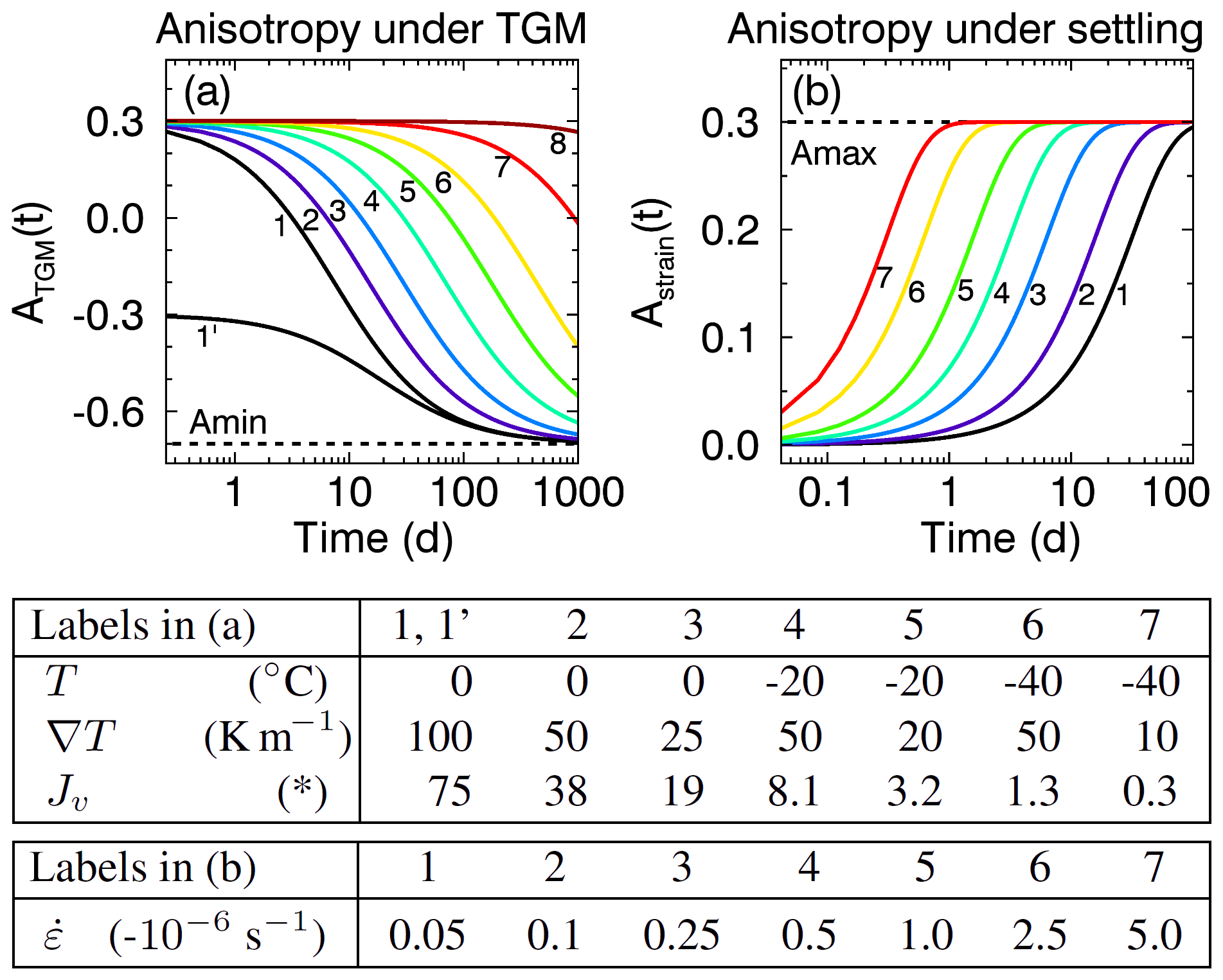
Figure 2 Modeled anisotropy evolution for TGM with and settling with α2=1.68 for the different tabled conditions (1–7). In (a), 1 and 1′ differ only by the initial anisotropy. The dark red line (8) corresponds to and ∘C. The vapor flux Jv is given (*) in units of 10−8 kg m−1s−1.
2.6 Model behavior and numerical solution
The model is summarized in Fig. 2, which shows the anisotropy evolution for different parameters as obtained by numerical integration of the rate equation using the explicit Euler method (no difference was observed for the classic Runge–Kutta method). Depending on temperature, the timescales of the anisotropy evolution under TGM (Fig. 2a) range between 10 and 300 d because the water vapor flux can vary by 2–3 orders of magnitude (table below Fig. 2). Extreme values close to Amin are only reached after hundreds of days. The comparison of the two runs (1) and (1′) shows that for the same temperature settings negative anisotropies evolve slower than positive anisotropies. The dark red line (8) shows that even when strong temperature gradients are applied for many years no significant anisotropy change can be observed under conditions used for sample archiving in the lab. Compared to TGM the settling-induced anisotropy (Fig. 2b) is modeled to evolve much faster (hours to days). As both the strain rate and the A2 terms in Eq. (13) are always negative, snow settling always increases the anisotropy. The particular choice for the upper and lower limits of the anisotropy, namely and Amax=0.3, will be further discussed below.
A comprehensive set of laboratory and field data was used to calibrate, drive, and evaluate the model. Here, we describe the different datasets and the forcing, calibration and evaluation of a large ensemble of SNOWPACK runs.
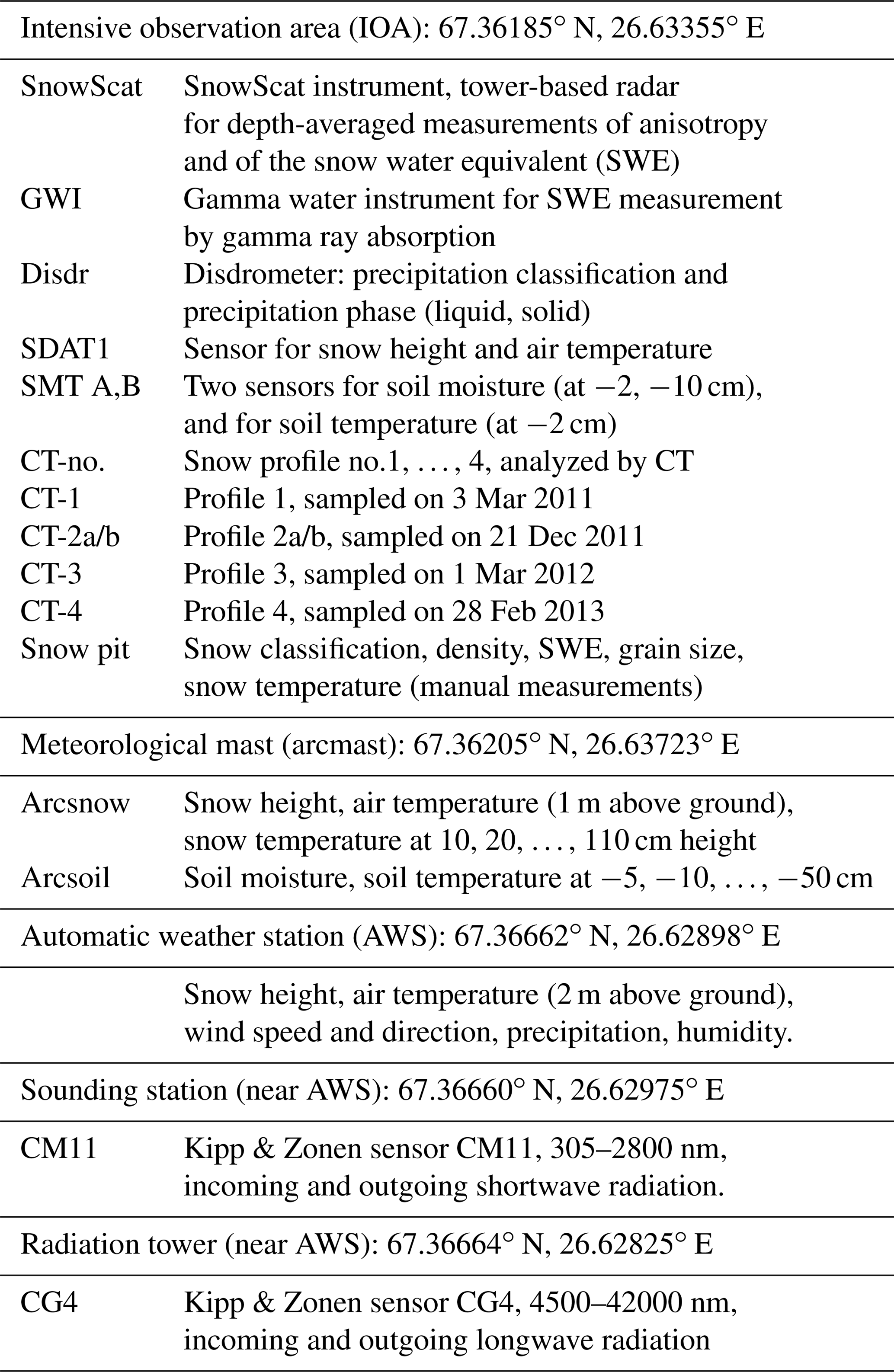
Except for an independent set of laboratory CT data, all field data were acquired in northern Finland 5 km south of the town of Sodankylä at or close to the test site “intensive observation area” (IOA). The IOA is shown in Fig. 3. Table 2 lists all measurements, sensors, and their locations. The measurements were supported by the Nordic Snow Radar Experiment (NoSREx-I to NoSREx-III) (Lemmetyinen et al., 2013, 2016).
At the IOA, snow pit measurements were performed on a weekly basis. The measurements include snow temperature and snow classification. In addition near-infrared (NIR) images of the snow structure were taken on selected dates. For each NIR image we calculated the ratio to a reference image of a Styrofoam panel. The ratio images were used to cross-check CT data and snow type classification and for interpretation of the modeled results.
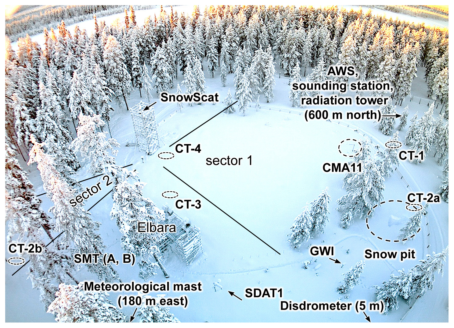
Figure 3All field, all radar, and most meteorological data were acquired at the intensive observation area (IOA). The remaining meteorological data were measured at the meteorological mast 180 m east of the IOA and at the automatic weather station (AWS) 600 m north of the IOA. Anisotropy validation profiles were extracted at the locations CT-1, CT-2a/b, CT-3, and CT-4. The depth-averaged anisotropy for “sector 1” was measured every 4 h with a tower-based radar (SnowScat) which also measured the snow water equivalent in combination with the gamma water instrument, GWI, as detailed in Leinss et al. (2015). Sensor abbreviations are explained in Table 2.
3.1 Anisotropy determined by computer tomography
For validation of the model we used anisotropy data derived from 3-D scans of snow samples analyzed by X-ray microtomography (CT). Our analysis includes published data of time series acquired during temperature gradient metamorphism experiments in the lab and snow samples taken in the field during the NoSREx campaign.
The field samples were casted using diethyl phthalate (DEP) for transportation as described in Heggli et al. (2009) and scanned with a nominal resolution (voxel size) ranging between 10 and 20 µm. The resulting 3-D grayscale images were filtered using a Gaussian filter (sigma = 1.2 voxel length, total filter kernel width = 4 voxel lengths). The smoothed images were then segmented into binary ice–air images. For segmentation, an intensity threshold was chosen at the minimum between the DEP peak and the ice peak in the histograms of the grayscale images.
Two-point correlation functions were calculated from the binary images for each direction (Löwe et al., 2013). Then, the correlation lengths, pex,x, pex,y, and pex,z were derived as described in Mätzler (2002). Because of the symmetry in the x–y plane, the lengths pex,x and pex,y were averaged, and the corresponding CT anisotropy follows, analogue to Eq. (1):
To validate the anisotropy evolution under TGM and to determine the free parameter α1 we used the laboratory data listed in Table 1. The samples TGM-17 (Kaempfer et al., 2005), TGM-2 (Löwe et al., 2013), DH-1, and DH-2 (Riche et al., 2013) were analyzed for their exponential correlation lengths in Löwe et al. (2013). In addition we used digitized data of the sample C-1 analyzed by Calonne et al. (2014).
Table 1List of snow samples from laboratory TGM experiments with temperature, temperature gradient, initial ice volume fraction, initial snow type and sub-type, specific surface area (SSA), and duration of the experiment. The corresponding anisotropy evolution is shown in Fig. 5.

For validation of the full model applied on field-measured conditions, almost complete vertical snow profiles were extracted in Finland and preserved for later analysis in Switzerland. Five profiles named CT-1, CT-2a, CT-2b, CT-3, and CT-4, were sampled at the locations shown in Fig. 3 on the dates listed in Table 2. The structural anisotropy was determined with a vertical resolution of 1–2 mm. The profiles contain some gaps of a few centimeters where the samples were not overlapping or sample taking was not possible due to very soft new snow (CT-4), ice crusts, or large fragile depth hoar crystals (CT-1). Data of the profiles CT-2a and 2b were combined. Examples of the analyzed 3-D snow structure are shown in Leinss et al. (2016, Figs. 14 and 15). Other derived parameters have already been published in Proksch et al. (2015).
3.2 Anisotropy determined by polarimetric radar
Depth-averaged anisotropy time series were obtained from polarimetric radar measurements acquired by the ground-based radar instrument SnowScat. SnowScat was developed and built to analyze the backscatter intensity of snow between 9.2 and 17.8 GHz (Lemmetyinen et al., 2016), ESA ESTEC contract 42000 20716/07/NL/EL (available on request from ESA). Technical details of the instrument are given in Werner et al. (2010).
The method for measuring the depth-averaged anisotropy from radar data is detailed in Leinss et al. (2016). Here we briefly outline the method. Microwaves with a sufficiently long wavelength penetrate the snowpack with negligible scattering losses and accumulate a signal delay by the refractive index of snow. For snow with a spatially anisotropic microstructure the signal delay depends on the polarization of the electric field. The signal delay difference between two polarized radar echoes perpendicular to each other can then be precisely measured interferometrically by determining the co-polar phase difference, CPD (Leinss et al., 2016). From the CPD, the depth-averaged radar anisotropy, , can be derived when snow depth and density are known.
When this method is applied at sufficiently high frequencies (10–20 GHz), can be determined with an accuracy of a few percent. The frequency limits are determined such that the radar penetration depth in snow is sufficiently high (upper limit), the system's phase accuracy is much smaller than the total measured CPD, and the penetration into soil (and polarimetric effects of soil) is negligible (lower limit).
About 3200 anisotropy measurements with a temporal resolution of 4 h were acquired at the IOA during the four winter seasons 2009–2013. The anisotropy measurements were taken for 13 frequency bands (bandwidth of 2 GHz) covering the full frequency spectrum of SnowScat (9.2–17.8 GHz). Because the CPD is rather small for the incidence angle , we used only anisotropy measurements made at θ=40, 50, and 60∘. To reduce phase noise, CPD measurements from 17 different azimuth angles were averaged before derivation of the anisotropy. Because microwaves frequencies above 10 GHz have almost no penetration into wet snow, the anisotropy during snowmelt could not be measured.
3.3 Anisotropy determined by SNOWPACK
For comparison of modeled results with radar data and to simulate the depth-resolved anisotropy evolution, we forced the anisotropy model with snow properties simulated by the model SNOWPACK (v. 3.4.5). The model was forced by meteorological and soil data and was calibrated with snow height and snow temperature measurements. The following subsections provide intermediate details of the retrieval, preprocessing, and filtering of these measurements. More details are provided in Appendices A1 and A2. Plots of input, output, and control data of SNOWPACK are provided in the Supplement.
Table 2List of field data for model input, calibration, and validation. For each site, sensor abbreviations and full sensor names, or dataset abbreviation and type of measurements, are given.
3.3.1 Meteorological data
For the snow–atmosphere boundary conditions, SNOWPACK requires the following meteorological input data: air temperature (TA), soil temperature (TSG), relative humidity (RH), wind speed (VW), wind direction (DW), incoming shortwave radiation (ISWR) and/or reflected (outgoing) shortwave radiation (OSWR), incoming longwave radiation (ILWR) and/or snow surface temperature (TSS), precipitation (PSUM) and/or snow height (HS), and optionally the precipitation phase (PSUM_PH). For monitoring purposes, up to five internal snow temperature measurements (TS1, …, TS5) at different heights can be provided for comparison with modeled snow temperatures. Most input data were measured redundantly by more than one sensor at the IOA (Table 2). Precipitation and wind velocity were measured at the automatic weather station (AWS), 600 m north of the IOA. The radiation balance was measured close to the AWS at the sounding station and at the radiation tower. A very similar, well-calibrated dataset is available by Essery et al. (2016).
To provide physically correct and consistent conditions, the meteorological data were filtered, combined, and interpolated if gaps could not be filled with equivalent datasets (details in Appendix A1). Plots of both measured raw data and filtered SNOWPACK input data are provided in the Supplement Figs. S3–S10. SNOWPACK additionally filters and preprocesses the input data and provides them for control (Figs. S11–S14).
3.3.2 Soil data
For the lower boundary condition, SNOWPACK requires a description of at least one soil layer. To precisely define the temperature of the soil–snow interface we defined a single, 5 cm thin soil layer whose lower temperature (TSG) was provided by the average of four soil temperature sensors at −5 and −10 cm (sensor: arcsoil at meteorological mast) and two measurements at −2 cm depth (sensor: SMT at IOA).
For soil moisture we averaged data from six sensors, two from the meteorological mast (arcsoil: −5, −10 cm) and four from the IOA (SMT A and B, each at −2 and −10 cm). Soil moisture and temperature were provided averaged over 1 week around the simulation start time (1 September).
The soil composition is described in Lemmetyinen et al. (2013) as very fine mineral soil composed of 70 % sand, 1 % clay, and 29 % silt. For this mineral soil, we assumed a solid volume fraction of 75 % and zero ice fraction in autumn. We estimated a density of 1800 kg m−3, a heat conductivity of 1.5 W m−1 K−1 (from ToolBox, 2003a), and a heat capacity of 1000 J kg−1 K−1 (from ToolBox, 2003b). A soil albedo of 0.2 was determined from the ratio of incoming and reflected shortwave radiation data.
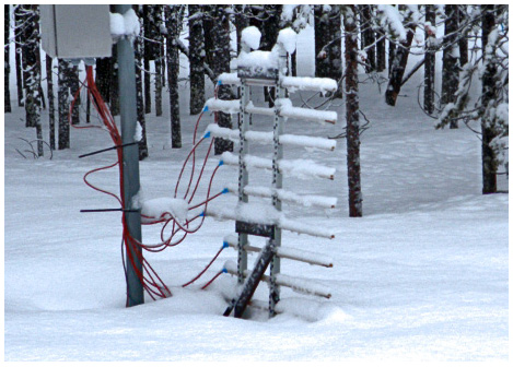
Figure 4Snow temperature was measured with an array of horizontally oriented temperature sensors at the meteorological mast. Image modified after Lemmetyinen et al. (2013).
3.3.3 Snow temperature data
Snow temperature, used for SNOWPACK calibration, was measured at the meteorological mast, 180 m east of the IOA, with an array of 11 horizontally oriented temperature sensors located at 10, 20, …, 110 cm above the ground (Fig. 4).
Unfortunately, for this configuration with all sensors attached to the same support stick, we cannot exclude that some air-filled gaps occurred between the sensor elements. Furthermore, it was reported for another, similar sensor configuration that the sensor configuration interfered with snow accumulation and caused the formation of an up to 30 cm deep pit in the snow around the sensor. Such sensor biases can be detected by comparing the lowest snow temperature (at +10 cm above ground) with the measured soil temperature (see Fig. S17), because for a deep, well-insulating snowpack, both temperatures should not vary more than a few kelvin. Manual snow temperature measurements provide an additional validation source for the sensor array measurements.
3.3.4 Calibration and configuration
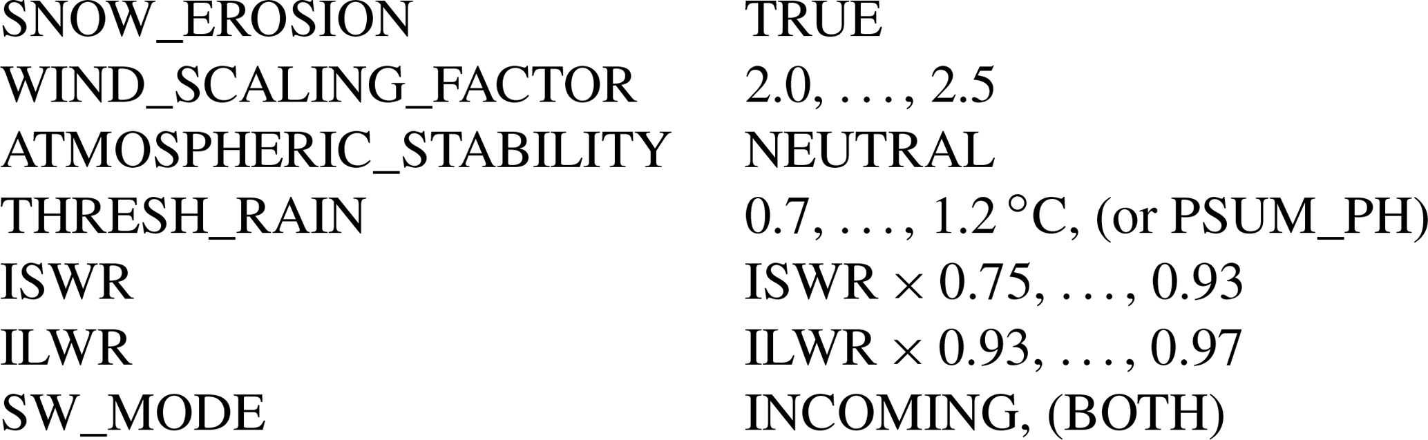
SNOWPACK provides a variety of settings to adjust for the local environment and to configure the simulation. Additionally, the radiation balances required some calibration because it was not directly measured at the IOA. To best replicate measured snow height and temperatures, we run for all four seasons more than 5000 simulations with different settings each time (but keeping the same settings for all four seasons) and graded the accuracy of the simulation results by comparison of simulated snow height and snow temperature with measured snow height and temperature (details in Appendix A3). To avoid systematic deviations of SWE or snow density, we first run SNOWPACK driven by calibrated precipitation (Appendix A1). Then, we run the best 237 simulations again but with enforced snow height; i.e., SNOWPACK tries to estimate the precipitation which is required to reproduce the measured snow height. For a sanity check we verified the simulated SWE. Table 3 summarizes the most important settings which improved the simulation results significantly. Little difference was found between a fixed threshold for the precipitation phase (THRESH_RAIN) and estimation of the precipitation phase (PSUM_PH) from disdrometer data (Appendix A1). When enforcing snow height, snow height was better predicted but SWE was slightly overestimated when reducing the default value HEIGHT_ NEW_ ELEM = 0.02.
Tree canopy was not considered (CANOPY = FALSE) because the test site was not covered by trees. Still, surrounding trees could have affected the radiation balance which was calibrated by multiplication with constant factors and selection of the best simulation results. Incoming shortwave radiation (ISWR) was reduced (Table 3), which agrees with the fact that the IOA was partially shadowed by trees but shortwave radiation was measured on a tower above the trees. Outgoing shortwave radiation (OSWR) was internally estimated by SNOWPACK based on the simulated albedo (SW_MODE = INCOMING instead of BOTH). The incoming longwave radiation (ILWR) needed only a little reduction. Outgoing longwave radiation was not used by SNOWPACK. The reduction of shortwave radiation agrees with the model by Essery et al. (2016); however, they modeled an increase in the longwave radiation by a few percent whereas we reduced it by a few percent such that SNOWPACK results agree better with snow depth and temperature measurements.
Table 3Most relevant settings for SNOWPACK which produced the best results.
3.3.5 Coupling the anisotropy model to SNOWPACK
The proposed model for the anisotropy is designed for immediate implementation into snowpack models which provide the following variables for each layer of snow: snow temperature T, vertical snow temperature gradient , and strain rate . SNOWPACK provides these parameters but does not consider the structural anisotropy of snow. To keep the implementation simple enough, we post-processed the output of SNOWPACK and did not intend to feed the anisotropy back into SNOWPACK.
SNOWPACK merges two adjacent snow layers when they have similar properties and when their thickness falls below a certain threshold. To keep track of the anisotropy evolution of merged layers, we wrote an algorithm to detect when snow layers get merged. We defined the anisotropy of a merged layer by the average anisotropy of the two original layers weighted by their thickness.
Extremely large temperature gradients could naturally occur at the snow surface under extreme conditions but we do not expect that the anisotropy will grow proportionally to such extreme gradients. Extreme temperature gradients could also wrongly occur in simulated data. To exclude such temperature gradients, we set a maximum threshold for simulated temperature gradients of K m−1.
3.3.6 Ensemble runs
To consider the uncertainty of different SNOWPACK configurations, we run a sensitivity analysis of the model and determined α2 for the ensemble of the best 237 SNOWPACK simulations. Each ensemble member consists of four seasons simulated with the same SNOWPACK configuration. For each ensemble member, α2 was determined once for each season independently and once for all seasons together. The ensemble members differed slightly in the following configuration settings: scaling of radiation balance, rain threshold, wind scaling factor, shortwave reflected radiation based on albedo simulation or measurements, precipitation phase estimation, and different thresholds for the height of new snow elements (5 mm, 1, 2 cm). All 237 simulations had the following settings in common: snow height was enforced, atmosphere was neutral, and snow erosion was allowed. An analysis of the accuracy of the corresponding SNOWPACK ensemble members is shown in Fig. S19.
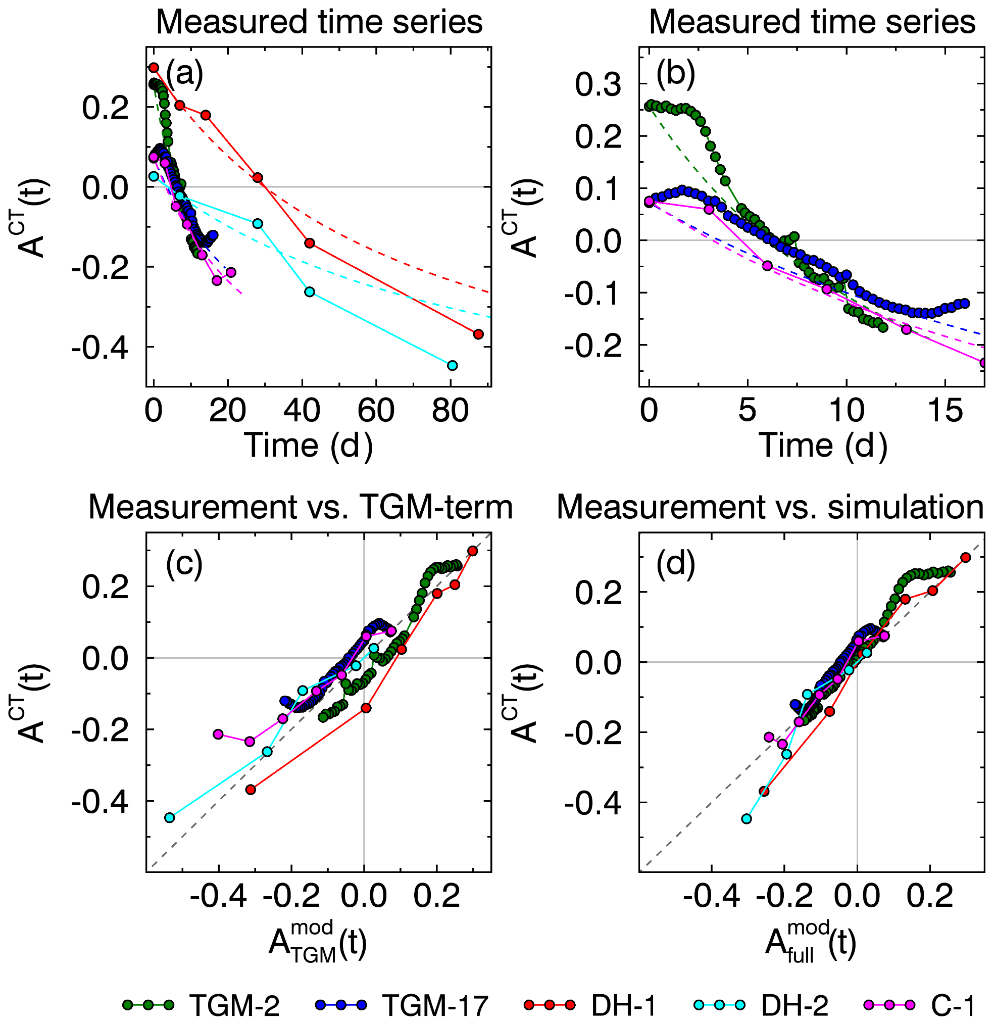
Figure 5(a) Anisotropy time series ACT(t) of the laboratory experiments from Table 1. Dashed lines indicate modeled results. (b) Zoom into the first 15 d after the start of the experiment. (c) When ignoring the lower threshold Amin and with the simulated data already agree well with CT data. (d) With a lower threshold and with , the agreement of model and measurements indicates that the growth of vertical structures is proportional to the water vapor flux.
4.1 Validation by laboratory experiments
For validation of the TGM formulation we analyzed anisotropy time series from the five laboratory CT experiments listed in Table 1. The time series are shown in Fig. 5a and b. All experiments indicate that the anisotropy did not reach a stationary value at the end of the experiment but would further decrease with time. Extrapolating the curves would probably reach a stable state around , which indicates that Amin must be smaller than the lowest observed value of −0.45. Therefore, we choose a practical minimum threshold of . We note that such low values have been observed in neither lab experiments nor nature, because the experiment would need to last many hundreds of days and in nature snow would either evaporate or TGM would occur combined with settling.
A simple check of anisotropy evolution with respect to the vapor flux dependence can be done when ignoring the limiting factor in Eq. (5) and setting . By time integration one obtains , which agrees well with the experimental data as shown in Fig. 5c. Because the laboratory CT data were obtained with different temperatures and temperature gradients (Table 1), this relation indicates that the growth of vertical structures is almost linearly dependent on the vapor flux Jv. Then we applied the full Eq. (5), including the limiting factor with , which yields by minimizing the RMSE (= 0.048) between the laboratory CT data and the simulated data. Figure 5d shows a slight improvement of the results compared to Fig. 5c.
An interesting detail appears in Fig. 5(b) at an early stage. The anisotropy seems to be quite stable for a few days and vertical structures do not start growing before 2–3 d after the start of the experiment.
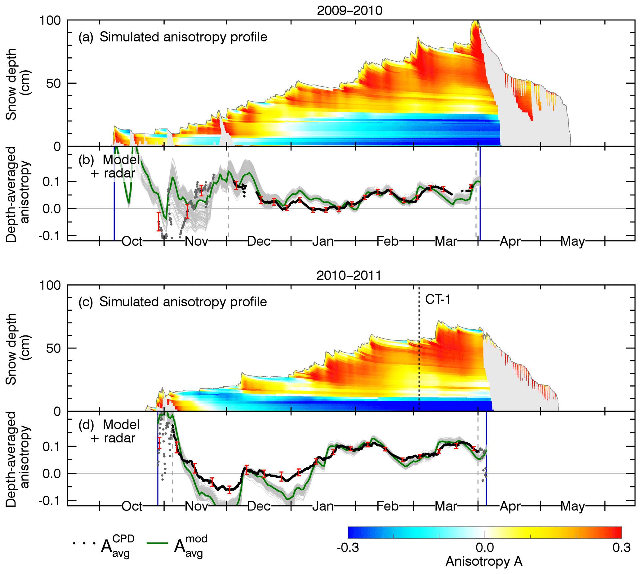
Figure 6Structural anisotropy simulated for the first two seasons 2009/2010 and 2010/2011. (a, c) Depth-resolved anisotropy (in color) based on post-processed SNOWPACK data with model parameters , α2=1.68, , and Amax=0.3. Wet snow is grayed out. The sampling date of the validation profile CT-1 is indicated by the dashed line. (b, d) Modeled, depth-averaged anisotropy (green: ensemble median; gray: ensemble members) and radar-measured anisotropy used for calibration of α2 (black). Gray dots indicate radar measurements excluded from calibration because of a too big standard deviation (red error bars).

4.2 Seasonal evolution of the anisotropy
No laboratory data about the anisotropy evolution of new snow are presently available. Therefore, we calibrated the parameter α2 by running the full model on the output of SNOWPACK and compared the depth-averaged anisotropy measured by radar with the depth-averaged anisotropy of the model results.
The radar-measured anisotropy time series, , are shown in the lower panels (b, d) of Figs. 6 and 7 as a line of solid black dots. The corresponding standard deviation of radar measurements acquired with different frequencies and incidence angles of the radar antenna is indicated by red error bars. Radar measurements were considered reliable enough for model calibration when the snowpack was dry and the standard deviation was below 0.05. Gray dashed lines limit the radar measurements used for model calibration; radar measurements excluded from calibration are shown as gray dots. The beginning and the end of the period considered to be the dry snow period are indicated by vertical blue lines. During the dry snow period, a few short melt events can be recognized in the depth-resolved anisotropy profiles as gray areas.
In the radar measurements the maximum anisotropy never grows much beyond +0.2, even in December 2011 where air and soil temperature were around 0 ∘C so that the growth of vertical structures by TGM was limited and mainly settling of the thick snowpack occurred. From that we estimate the value for and used this value in the model.
The depth-resolved, modeled anisotropy is shown in color in the upper panels, (a) and (c), of Figs. 6 and 7. Yellow and red indicate horizontal structures and shades of blue indicate vertical structures. The model is based on the output of the best snowpack simulation. As we do not model the anisotropy evolution of wet snow, wet snow is grayed out. When the simulated anisotropy profiles are vertically averaged one obtains the simulated, depth-averaged anisotropy, , which is shown as a green line in the lower panels, (b) and (d).
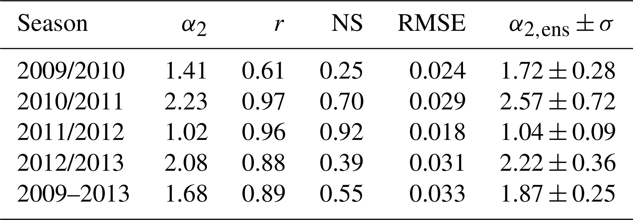
To evaluate the uncertainty of the free parameter α2 we determined it for each season independently and also for all seasons together by minimizing the RMSE between and . In addition to the RMSE, the model accuracy was measured with the Nash–Sutcliffe model efficiency coefficient and also with the Pearson r correlation coefficient. Table 4 summarizes the results. The depth-resolved profiles and depth-averaged time series in Figs. 6 and 7 show the results for α2=1.68 determined for all seasons together, which results in an RMSE of 0.033 and a Pearson r correlation coefficient of 0.89.
Table 4Results for the parameter α2 determined for each season independently and for all seasons together. The agreement between model and radar anisotropy is given by the Pearson's correlation coefficient (r), the Nash–Sutcliffe model efficiency coefficient (NS), and the root-mean-square error (RMSE). The last row contains the mean and standard deviation of α2 from the ensemble runs.
The sensitivity of α2 on slightly different SNOWPACK settings is represented by the ensemble of gray lines in panels (b) and (d) of Figs. 6 and 7. The last column of Table 4 summarizes the ensemble results. The ensemble of gray lines corresponds to where the uncertainty is specified by the standard deviation.
Considering that it is a hypothesis that settling increases the anisotropy, it is remarkable that the modeled anisotropy and the radar-measured anisotropy show a highly consistent trend: the model is able to catch many details of the radar-measured anisotropy time series. Nevertheless, in some early winter periods, especially in the season 2010/2011, stronger deviations occur, likely because of melt events and differently modeled snow height and layer thicknesses.
From the simulated anisotropy profiles it is evident that snow layers at the bottom of the snowpack mainly show vertical structures (blue, A<0) while the upper snow layers (and the first snow every season), which are stronger affected by snow settling, show generally horizontal structures (yellow and red, A>0). An exception is the snow surface, which shows a more isotropic (and sometimes an even vertical) structure compared to the underlying upper snow layers which experienced more overburden pressure. The occasionally appearing vertical structures at the snow surface are expected from the strong temperature gradients at the surface, especially during clear-sky winter nights. During such conditions, TGM transforms the top layers faster than intermediate layers.
A small but very interesting detail, especially in the radar measurements, is that the anisotropy does not grow instantaneously with accumulating new snow but shows a delayed increase within a few days (e.g., in March 2010, March 2011, December 2011, and February 2013). We think this delay could result from a settling-related effect: initially fallen crystals have an intrinsic particle orientation which is not perfectly aligned horizontally when first sticking to the surface. Upon initial metamorphism and settling, which takes some characteristic time, these crystals may further align horizontally under the influence of gravity with a measurable impact on the anisotropy. The delay seems to be more pronounced in the radar measurements than in the model where the anisotropy often increases too quickly after snowfall. The length of this delay was determined to be about 2–4 d on average in Leinss et al. (2016, Sect. 5.4).
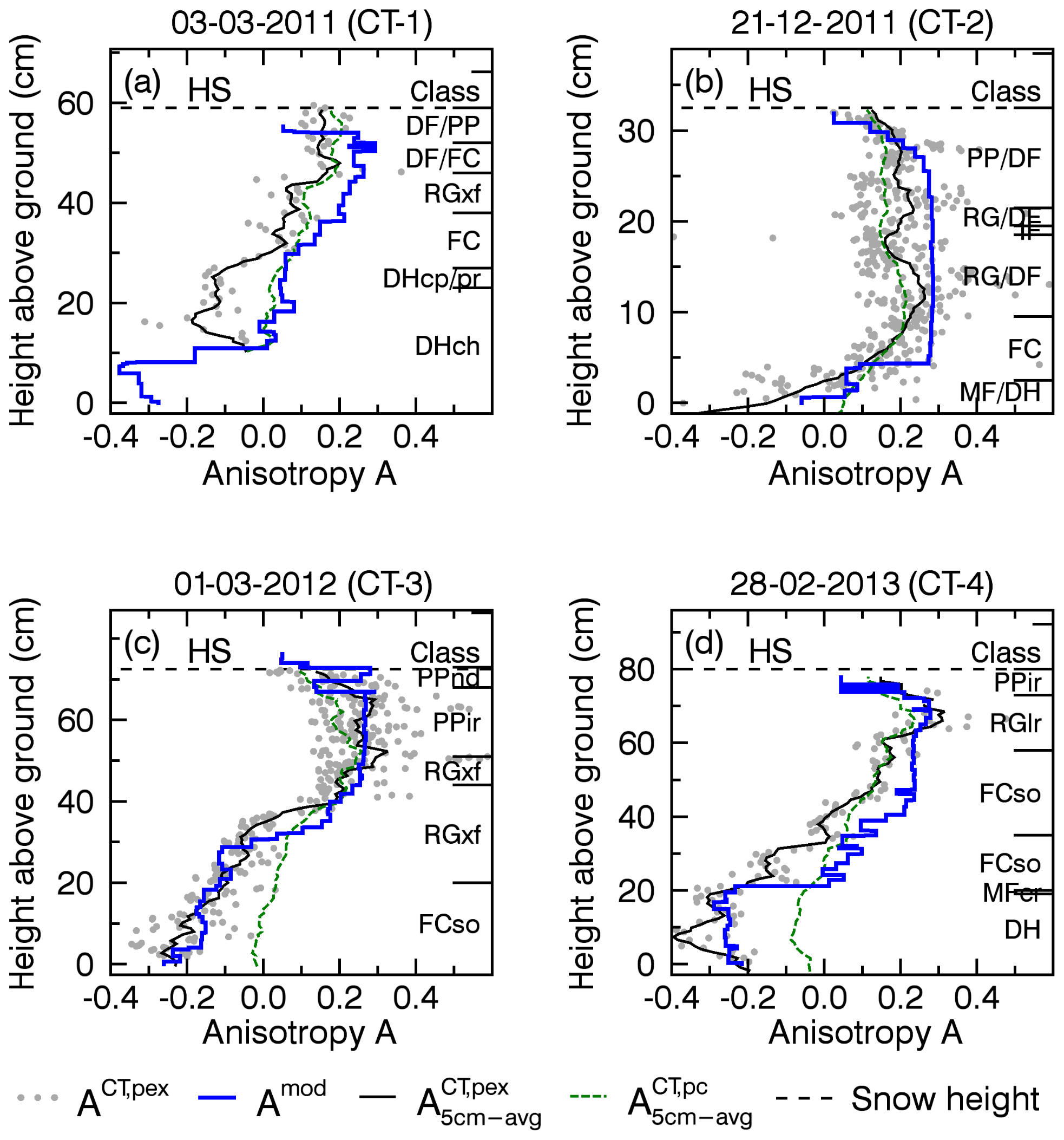
Figure 8Comparison of simulated anisotropy (Amod, blue line), with field-measured CT anisotropy profiles (, gray dots; black line: 5 cm running mean). Right axis: snow layer classification according to Fierz et al. (2009) and measured snow height (HS, horizontal black dashed line). The anisotropy determined from the correlation length pc is shown as a green line (5 cm running mean). The locations where the CT profiles were taken are shown in Fig. 3.
4.3 Validation with CT profiles from the field
The seasonally modeled depth-resolved anisotropy was validated with vertically resolved field-measured anisotropy CT profiles. The dates when the CT profiles were obtained in the field are indicated by vertical black dashed lines labeled with CT-1, CT-2, CT-3, and CT-4 in Figs. 6 and 7.
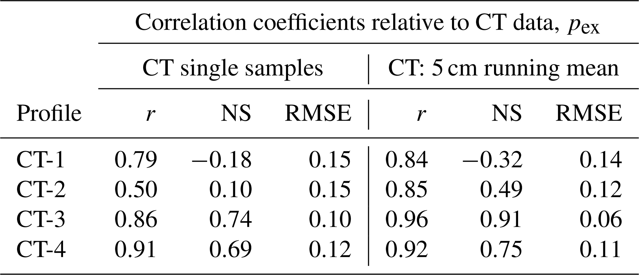
In Fig. 8 the modeled anisotropy profiles (blue lines) are compared to the CT-based anisotropy (gray dots; black line indicating the 5 cm running mean). Table 5 lists correlation coefficients between the modeled anisotropy and the individual CT anisotropy data points derived from pex (left columns) as well as the correlation coefficients with the 5 cm running mean of the pex-based anisotropy (right columns). For both, the Pearson r correlation coefficients are around 0.8 and higher except for CT-2 (r=0.50) for which the snow structure does not show much vertical variability except for a thin layer of depth hoar at the bottom of the snowpack. Unfortunately for CT-1, Fig. 8a, no snow samples were taken for the lowest 10 cm for which the lowest anisotropy values were modeled. The most positive anisotropy values in the CT data of A=0.3 with some scatter up to 0.4 and higher agree with our estimation of .
Table 5Correlation coefficients between modeled anisotropy profiles and CT anisotropy profiles as shown in Fig. 8. The first three columns are the correlation with respect to the individual anisotropy data points; the rightmost three columns are correlations with respect to the 5 cm running mean of the CT-measured anisotropy.
4.3.1 Anisotropy determined from pc
In general, the anisotropy could also be calculated from other correlation lengths. For example, the anisotropy is derived from pc which is defined by the slope at the origin of the correlation function. By definition, pc describes characteristics on the smallest length scales, e.g., the specific surface area (Löwe et al., 2011), and is not sensitive to the extent of large structures. Therefore, (green dashed line in Fig. 8) indicates a less distinct anisotropy than . Especially for depth hoar, where both anisotropies differ most, the often used relation pex≈0.75pc is not valid (Mätzler, 2002; Krol and Löwe, 2016) and we obtained rather a relation of pex≈0.8…1.2pc (Fig. S1). The comparison of the anisotropy profiles based on pex and pc shows that pex is more sensitive to characterize the anisotropy.
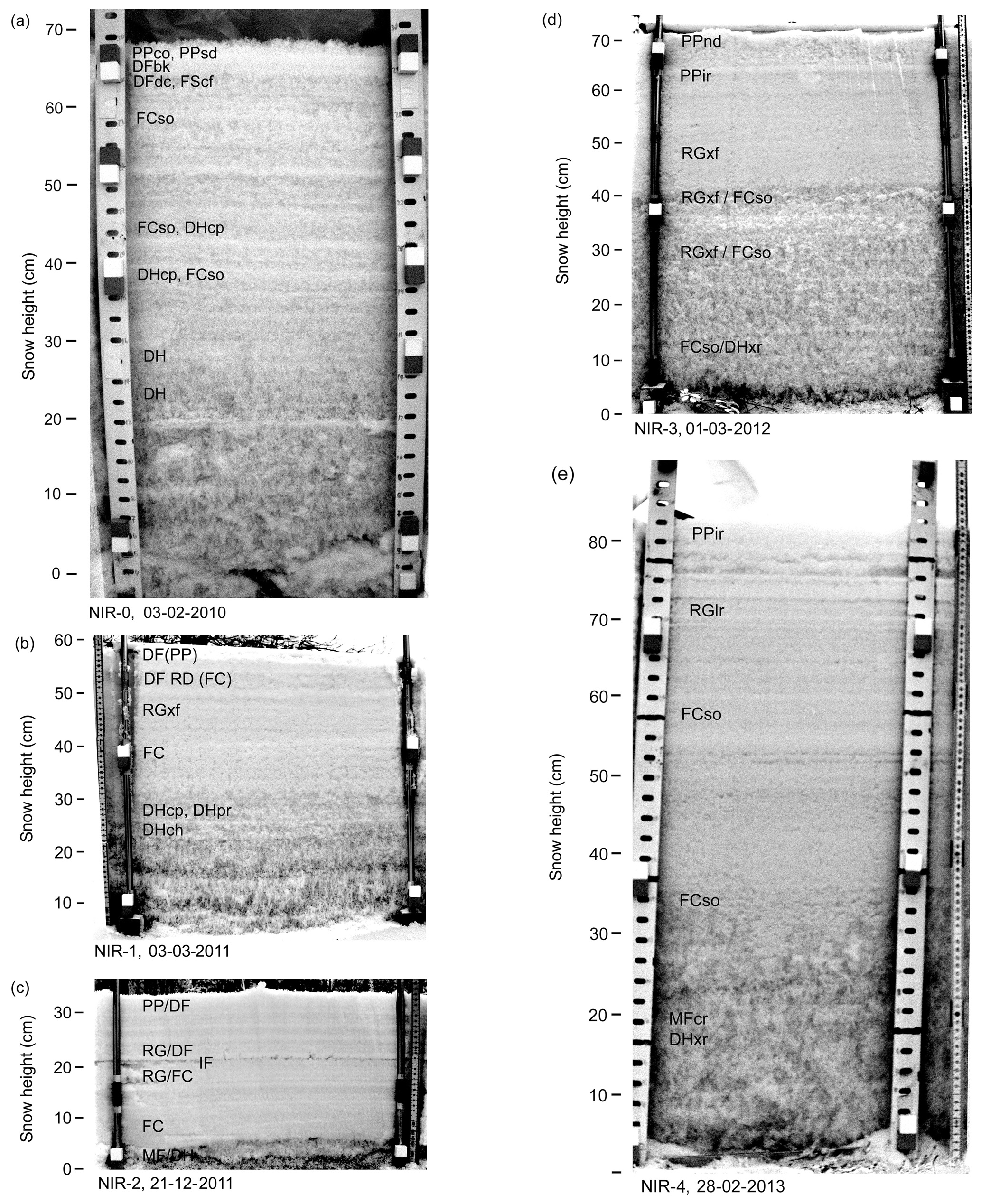
Figure 9NIR photography of the snowpack. The image NIR-0 was acquired in the first season on 23 February 2010 where no CT data are available. The other images NIR-1, NIR-2, NIR-3, and NIR-4 correspond to the CT profiles CT-1, CT-2, CT-3, and CT-4. The intensity of the NIR photography is mainly determined by grain size but also shows the metamorphic state of the snowpack. The NIR photography provides an independent measure for the absolute depth of individual snow layers and helps to identify strong structural transition in the snowpack.
A main motivation of this paper was to show that it is possible to model the radar-measured anisotropy solely based on meteorological data. This was achieved in detail and demonstrates that polarimetric radar measurements at sufficiently high frequencies (10–20 GHz) can be used to monitor the depth-averaged evolution of the anisotropy nondestructively (Leinss et al., 2016) and even from space (Leinss et al., 2014). Beyond that our results confirm that the creation of vertical structures is mainly controlled by the recrystallization rate of water vapor. The results further indicate a yet undocumented effect of settling on the creation of horizontal structures. It is remarkable that the model, which completely neglects any grain size parameter like SSA, is able to predict the temporal evolution of a microstructural parameter, the anisotropy, solely based on macroscopic fields and with a very limited set of free parameters which we determined from laboratory CT data and radar measurements.
5.1 Seasonal model results and snow conditions
Snow conditions observed in the field differed significantly between the different winter seasons; therefore, we provide a short summary for every season before discussing the evolution of the simulated and radar-measured anisotropy with respect to observed snow and weather conditions. For reference, snow height, air temperature, and soil temperature are plotted in Fig. 10.
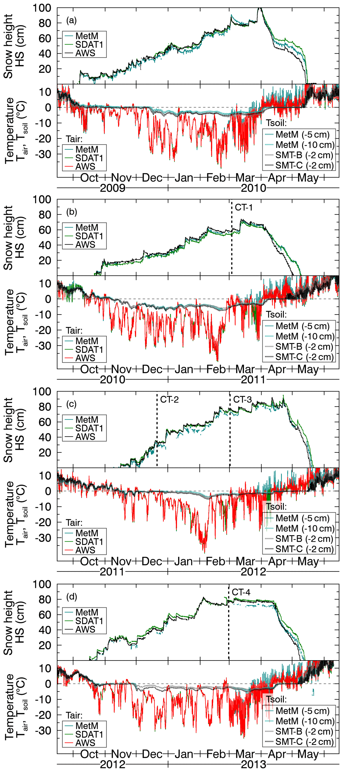
Figure 10Snow height and air and soil temperature at different locations (IOA, AWS; MetM is meteorological mast).
In the first season, 2009/2010, snowfall started in early October and accumulated up to 30 cm during relatively moderate temperatures (and some short melt events) until the middle of December when temperatures dropped well below zero and the soil froze.
The corresponding modeled mean anisotropy varies strongly in October–November, Fig. 6b, where model and radar data disagree because microwave penetration was reduced by temporary melt events, gray in Fig. 6a, and melt metamorphism was not considered in the model anyway. The precision of the radar measurements was also limited by the 10–15 cm thin snowpack. After the middle of November new snow dominates the modeled anisotropy which then agrees better with the radar measurements. At the end of December cold temperatures transformed the early winter snowpack into vertical structures. Each of the following snowfall events temporarily increased the average anisotropy, Fig. 6b. The NIR image from 23 February 2010, Fig. 9a, confirms the model results of metamorphic snow (depth hoar) in the lower 30 cm of the snowpack and shows multiple distinguishable layers above. No CT validation data are available for the first season.
In the second season, 2010/2011, conditions are characterized by a shallow snowpack with less than 30 cm of snow until January, accompanied with cold temperatures. The soil froze already in the middle of November and a layer of 20 cm depth hoar was present during the entire season.
The modeled mean anisotropy, Fig. 6d, clearly shows vertical structures until January but the radar data indicate a less strong anisotropy. During this period, the uncertainty of the radar data, indicated by the standard deviation (≈0.03, red error bars), is higher compared to other periods which could hint at some systematic measurement errors (Sect. 5.3). The modeled, depth-resolved results show that these vertical structures persisted through the entire winter season. In the NIR image, Fig. 9b, these structures appear as a 20 cm thick depth hoar layer at the bottom of the snowpack, which could not be sampled for CT analysis due to its brittle structure. For the upper 50 cm, the model overestimates the CT-measured anisotropy but still agrees with the general trend of the CT data from 3 March 2011, Fig. 8a.
In the third season, 2011/2012, snowfall started late but with intense snowfall 50 cm of snow accumulated in December during very mild air temperatures, often above −5 ∘C. Except for a few days in early December, TGM was almost not present and field measurements report finer grain size compared to other winter seasons (Leppänen et al., 2015). Then, between January and early February, temperatures dropped gradually from −10 to −30 ∘C and strong TGM set in which transformed the finely grained snow visible in Fig. 9c into the faceted crystals shown in Fig. 9d.
The modeled mean anisotropy and also the radar measurements show the highest observed values, , because in December vertical structures were almost completely absent. Only a thin layer of depth hoar is visible in the modeled results, Fig. 7a, which is confirmed by NIR and CT data, Figs. 9c and 8b. With the strong TGM in January–February, the initial snowpack transforms quickly into a 30 cm thick layer with vertical structures which emerges as a strong anisotropy reversal in Fig. 7b. Then, in the middle of February, an additional 30 cm of new snow fell on top of the transformed layers, resulting in the steplike anisotropy transition in the profile CT-3 shown in Fig. 8c. Until April, several minor snowfall events appear as little oscillations in the depth-averaged and radar-measured anisotropy, Fig. 7b.
At the end of the third season, gray snow layers appear in Fig. 7a from 10 to 13 April 2012 after accumulation which indicate that wet snow and rain fell on top of the snowpack, which partially refroze afterwards. The event induced strong settling in the SNOWPACK model which in turn increased the modeled anisotropy (green line, ). In contrast, the radar measurements reach zero for a moment (no penetration into wet snow) but returned to the previous values . We think that the anisotropy increase induced by settling was compensated by an anisotropy reduction from melt metamorphism which is currently not included in the model.
In the last season, 2012/2013, conditions are characterized by four major snowfall events. During the first event in November occasionally surface melt occurred. After the last event in February, very little precipitation was measured and cold temperatures persisted until early April.
The modeled mean anisotropy in November is above +0.2, but because of frequent surface melt no reliable radar measurements were possible (gray dots in Fig. 7d). Still, for a few days in the middle of November, anisotropy values up to +0.2 are visible in the radar measurements but they quickly approached zero, likely because of decreasing microwave penetration into wet snow. With very cold temperatures around −20 ∘C at the end of November, the snowpack refreezes and the positive anisotropy recovers but then quickly decays due to strong TGM, resulting in a 30 cm thick layer of depth hoar which continued to evolve during the remaining season, Fig. 7c. This depth hoar layer reached the lowest anisotropy values observed in the field as shown in CT-4 in Fig. 8d.
Interesting in March and April 2013, and also in other seasons, are the modeled vertical structures at the snow surface. These result from strong temperature gradients at the snow surface which does not experience any overburdened pressure and can therefore quickly transform into vertical structures or possibly surface hoar as classified by SNOWPACK (Figs. S20).
5.2 Quality of meteorological input data
For the best modeled anisotropy results it is critical that both meteorological input data and snow properties simulated by SNOWPACK are as correct as possible. For most of the meteorological data this was ensured by using redundant sensors; only precipitation was adjusted by SWE measurements (details in Appendix A1; for raw data see Figs. S3–S6). The results of SNOWPACK were assessed with snow depth and snow temperature.
For February 2011 we noticed that when air temperatures dropped below −30 ∘C measured snow temperatures were 10–20 K lower than modeled snow temperatures (black vs. red lines, second column in Fig. S17). We think that this is a measurement error because temperatures 10 cm above ground should not deviate strongly from measured soil temperatures, especially below a 60 cm thick snowpack. Similar for February 2010, snow temperatures measured 50 cm above ground were 10 K lower than modeled temperatures. The reason could be a few centimeters deep snow pit at the sensor array as mentioned in Sect. 3.3.3. Fortunately, for both events, modeled temperature at the bottom of the snowpack agrees closely with measured soil temperatures (red vs. gray line, second-to-last row in Fig. S17). Hence, we are confident that SNOWPACK simulated quite reasonable snow temperatures.
Snow temperature, especially in the upper layers, is strongly affected by the radiation balance which in turn affects settling, snowmelt, and TGM. Therefore, wrongly interpolated gaps in the radiation data cause deviations in the modeled anisotropy. For example, in the first season, several gaps of multiple days in the longwave radiation data between December 2009 and January 2010 were interpolated. Likely, too high incoming longwave radiation in the first week of January 2010, resulting in modeling of a too warm snow surface, could explain why the anisotropy in January 2010 did not decrease as indicated by the radar measurements, Fig. 6b. In the second season, several gaps of multiple days in the longwave radiation data between November 2010 and January 2011 seem to be correctly interpolated as both snow height and SWE agree very well; nevertheless, the simulated anisotropy deviates from the radar data. In the third season, radiation data were complete during winter. In the fourth season, the radiation balance for the rain-on-snow event in late November 2012 was manually corrected (Appendix A2).
Missing shortwave reflection data were no problem, because shortwave reflection was estimated based on the simulated albedo. The incoming shortwave radiation data did not contain any significant gaps.
5.3 Precision of radar measurements
Deviations between model and radar data could result from measurement errors and assumptions in the electromagnetic model to derive the anisotropy from the CPD. Uncertainties in the radar data could affect the strain parameter α2 and Amax. Of these, only α2 was solely determined by radar whereas the value for Amax is also constrained by CT data.
The uncertainty of α2=1.0…2.5 results very likely from model deficits rather than from radar measurements. The anisotropy measured with radar at different frequencies and incidence angles agrees within the standard deviation (shown in Figs. 6 and 7) with the underlying model (Leinss et al., 2016, Sect. 5.2). Systematic errors could result from uncertainties of the snow depth, especially for a very thin snow cover, but these measurements were excluded from model calibration. Systematic errors could also result from snow density estimations which, however, would result in an anisotropy error of less than 10 % (Leinss et al., 2016, Fig. 3).
5.4 Anisotropy model deficits
As a first approach, we avoided the inclusion of any other microstructural parameter in the anisotropy model. A more sophisticated description may discern different grain types, shapes, and sizes and its potential impact on the transformation into vertical structures. The microstructure is only reminiscent in the quadratic dependence (A−Amin)2 of the change rate which causes horizontal structures to transform much faster than vertical structures. Further, and similar to SNOWPACK, we did not consider any coupling between TGM and settling as observed by Wiese and Schneebeli (2017). Instead we fitted the free parameter α2 to radar data and determined the uncertainty α2≈1.0…2.5 by independent fits for each season and for different SNOWPACK ensemble members (Table 4). As the settling rate depends on the resistance of the bonded ice matrix to compression and as the resistance should depend on the anisotropy we think that α2 may contain a higher-order dependence on anisotropy. However, to keep the number of free parameters small we have used a constant value for α2. Interestingly, and likely because of the bounds Amin and Amax, model results do not differ significantly within the uncertainty range of α2 (compare Figs. 6 and 7 with Fig. A3 in Appendix). Therefore, we conclude that the mean value α2≈1.7 is a reasonably good approximation which can be used for most snowpacks. Varying the values of Amin and Amax within the estimated uncertainty range of ±0.1 does not affect the general dynamics of the model. Within this range the modeled results hardly changed more than ±0.05.
Our analysis is presently limited to the prediction of anisotropy from the output of a snowpack model (no feedback). If the (existing) feedback of the anisotropy onto mechanical properties of snow was allowed for, the parameters in the strain term will certainly change. We also point out that currently no comprehensive laboratory data exist which are able to confirm the predicted relation between settling of fresh snow and the creation of horizontal structures.
In the model we also neglected any melt metamorphism which could transform the microstructure very quickly. We think that for our Finnish data, melt metamorphism can be neglected as no strong melt events occurred except during the spring snowmelt where no radar data are available. Therefore, the calibration of a melt-metamorphism equation would lack sufficient calibration data. Nevertheless, we would like to propose a potential starting point for a model. Generally, one would expect that the rounding of ice grains in the presence of water drives anisotropic structures back to isotropy. In the absence of observations, one may refer to Lehning et al. (2002a) and Brun et al. (1992) and borrow a rate equation model for the anisotropy decay due to melt metamorphism in the form
with the empirical constant d−1 and the liquid water volume fraction in % Vol. Due to lack of sufficient data, we estimated the parameter α3 from the only event (April 2012) where refreezing occurred after strong surface melt. As a result, Eq. (15) induces almost isotropic conditions at the end of the melt season (Fig. S26).
Turning to the initial anisotropy Aini in the model, we assumed a constant value close to zero. Model results support this assumption and provide reasonable results for Aini between 0.00 and 0.05. The profiles CT-2 and CT-3, Fig. 8b and c, also show a slightly positive anisotropy, 0.05±0.05, for the surface layer 2–3 d after snowfall and support the assumption that the initial anisotropy must be small. Within the given range for Aini, a weak temperature dependence for Aini might exist, but no representative data are available. We think that stronger cohesion between crystals near the melting point could lead to a more isotropic structure (but with faster settling) compared to cold temperatures where crystals align rather by gravity and their anisotropic shape. A temperature dependence for the shape of snow growing in the atmosphere (Libbrecht, 2005) also influences the intrinsic anisotropy of crystals. This may have an impact on the subsequent evolution of the anisotropy in the snowpack since different crystals (e.g., dendrites and graupel as extreme cases) likely exhibit different settling rates and a different response to TGM.
Finally we note that the crystallographic fabric of snow, i.e., the angular distribution of the orientation of the c axis of the hexagonal ice crystals (the crystal lattice orientation), was also ignored. The c axis affects not only the dielectric anisotropy but also the crystal growth dynamics. For the radar data it was ignored because the crystallographic fabric (anisotropy) has a very weak effect on the dielectric anisotropy: ΔA≪0.02 (Leinss et al., 2016, Appendix A). For the model, we considered neither the evolution of the snow crystallographic fabric nor its influence on the evolution of the structural anisotropy. Only very few studies exist about the crystallographic fabric in snow (Calonne et al., 2016) or its evolution (Riche et al., 2013). Furthermore, the dominant growth direction of snow crystals depends on temperature (Lamb and Hobbs, 1971; Lamb and Scott, 1972) and is not necessarily parallel to the temperature gradient (Miller and Adams, 2009) as it can be clearly observed in Pinzer et al. (2012, Supplement movie). The competing effect of growth direction by crystal orientation versus structural optimization to increase entropy production by increasing the vertical thermal conductivity as suggested by Staron et al. (2014) might be a reason why a lower limit Amin of the anisotropy during TGM exists and why no perfectly vertically oriented snow structure has been documented so far.
5.5 An undocumented effect of settling?
From the radar time series a clear increase in the anisotropy a few days after snowfall is revealed in Leinss et al. (2016, Sect. 5.4) and also in Chang et al. (1996, Fig. 7). Likewise, spaceborne data indicate an increase in the CPD (and hence the dielectric anisotropy) proportional to the amount of new snow which must have settled after deposition (Leinss et al., 2014, Fig. 12). In our model this settling-induced creation of horizontal structures is well predicted by describing the anisotropy changes proportional to the strain rate. The modeled effect is however not independently confirmed yet and existing studies about the anisotropy evolution under strain provide very limited insight to confirm our hypothesis.
For example, Wiese and Schneebeli (2017) did not observe any significant growth of horizontal structures during compaction of relatively dense and coarse snow (, SSA = 13 m2 kg−1) which had also sintered for several months after initial sample preparation by sieving. Still, most samples showed a slight horizontal structure at the beginning of the experiment. Different to Wiese and Schneebeli (2017) and with the aim to study new snow of relatively low density ( and SSA = 70 mm−1 = 76 m2 kg−1), Schleef and Löwe (2013) avoided any sintering and observed indications for “the anisotropic nature of densification” by attributing observed density changes “solely to a squeeze of the structure in the vertical direction, i.e., to axial strains”. The affine compression in our model reflects this squeeze.
From our modeled results and from the above-described experiments and findings, we conclude that a so far undocumented effect during settling exists which creates horizontal structures, at least during an initial phase after new snow deposition. Unfortunately, a reanalysis of the dataset from Schleef and Löwe (2013) and Schleef et al. (2014) comprising 700 CT images is beyond the scope of the present study, also because the present calculation of the anisotropy from CT images may break down in new snow (see discussion below).
5.6 Anisotropy calculations from CT
Deviations between model and CT data could also result from ambiguities in the definition of anisotropy for a given microstructure. To understand this we recall that the relevant structural quantity for the dielectric tensor is a second-rank fabric tensor which is defined by an integral over the anisotropic correlation function of the material (Rechtsman and Torquato, 2008). Under the assumption that the correlation function possesses ellipsoidal symmetry, i.e., has the form C(r∕ℓ(cos θ)) with a single size scaling function ℓ(cos θ) that depends only on the polar angle θ, this integral can be exactly evaluated. The resulting fabric tensor can then be expressed in terms of the ratios of correlation lengths. If ellipsoidal symmetry was strictly true, any derived length scale (pex, pc,…) could be used for the anisotropy calculation and should lead to the same result. This is, however, not the case since Fig. 8 shows that the anisotropies based on the two correlation lengths pex and pc differ. On physical grounds, it is reasonable though that pex rather than pc is better suited to characterize the structural anisotropy for microwave measurements: pex characterizes the snow structure on length scales which are (still small but) closer to the wavelength of the radar. In contrast, density fluctuations on the smallest scales (namely those characterized by pc) solely characterize local properties of the ice–air interface (Löwe et al., 2011) which are irrelevant features for radar wavelengths. The experiments from Löwe et al. (2011) provide yet another hint for the violation of an (strict) ellipsoidal symmetry: it was shown the two-point correlation function contains at least two characteristic length scales which exhibit different ratios in different coordinate directions, again incompatible with the ellipsoidal form. In summary, there is evidence that the current (approximative) calculation of the anisotropy from a CT image using exponential correlation lengths is not equally well justified for different snow types. This may also explain observed differences between modeled and CT-based anisotropy and definitely needs to be taken into account in a potential future assessment of strain effects on the anisotropy evolution in snow.
In this paper, a model for the temporal evolution of the structural anisotropy of snow was designed. The model is based on simple rate equations and requires solely macroscopic fields as input variables, namely strain rate, temperature, and temperature gradient, ideally depth-resolved. These variables are provided by most of the more advanced snowpack models; here we used SNOWPACK.
To describe the evolution of the anisotropy, the model considers only two contributions: temperature gradient metamorphism (TGM), which was confirmed to create vertical structures, and snow settling for which we think that the strain leads to preferentially horizontally oriented ice grains in the snow microstructure. The TGM formulation was validated with existing CT data from laboratory experiments. The strain formulation was calibrated with 4 years of anisotropy data obtained from polarimetric radar measurements acquired in Sodankylä in Finland between 2009 and 2013. For calibration, we drove SNOWPACK with meteorological data and used the output to model the depth-resolved anisotropy. Then, we minimized the difference between the depth average of the modeled anisotropy and the depth-averaged radar anisotropy by adjusting a single-fit parameter. For sensitivity analysis the fit parameter was determined for each season separately but we also determined it globally for the entire set of all four seasons. Additionally, we run an ensemble of different SNOWPACK configurations to evaluate the model sensitivity to slightly different snowpack properties. We conclude that the same fit parameter can be used for any snowpack because model results improved only marginally when the parameter was adjusted for every season individually. Finally, the modeled, depth-resolved anisotropy profiles were validated with field-measured CT anisotropy profiles. The modeled anisotropy varies between values of about ±0.3 and agrees with the radar data with a root-mean-square error (RMSE) of 0.03 (Pearson ) and with CT data with an RMSE of less than 0.15 (Pearson ).
The results have immediate implications:
-
The model performance allows for improved parametrization of different snow properties like thermal, mechanical, and electromagnetic properties.
-
Our results indicate a yet undocumented effect of settling on the creation of horizontal structures in new snow.
-
The detailed agreement between the radar-measured anisotropy and the anisotropy modeled from meteorological data demonstrates that polarimetric radar measurements at sufficiently high frequency (10–20 GHz) can be used to monitor the evolution of the structural anisotropy.
The simplicity of the model facilitates an immediate implementation into common snow models to simulate the anisotropy, at least during dry snow conditions. We could show with laboratory CT data that for dry snow the growth of vertical structures is proportional to the vertical water vapor flux. Unfortunately, experiments with wet snow metamorphism at the melting point are difficult and only very few studies exist; therefore, we could only hypothesize about a formulation for the anisotropy evolution during snowmelt, which limits our model to dry snow applications.
The observation that the compression of new snow leads to horizontal structures may stimulate new laboratory experiments to reveal the mechanisms underlying the evolution of anisotropy in new snow and its feedback on mechanical properties as a function of crystal type. The fact that model, radar measurements, and CT data are consistent gives confidence in the interpretation of the radar-measured anisotropy. Depending on the system geometry, the anisotropy can only be measured depth-averaged (remote-sensing systems) or even depth-resolved with in situ systems as done for a fast characterization of firn cores (Fujita et al., 2009). Similarly, radar systems mounted on rails could be used to scan the snowpack layer by layer and nondestructively which allows for monitoring of the evolution of the depth-resolved anisotropy. Radar satellites can directly measure the co-polar phase difference (CPD) which is proportional to the depth-averaged anisotropy of a dry snowpack. For single radar acquisitions the CPD can be difficult to interpret and can even be zero for a snowpack with equal portions of layers with positive and negative anisotropies. In contrast, with radar time series, quantitative information, e.g., about new snowfall, can be obtained because we showed that the transformation by TGM is often slower than the anisotropy increase during accumulation of new snow (Leinss et al., 2014).
Finally, the large observation time spanning four winter seasons with a sampling interval of 4 h constitutes a unique data source to study the evolution of the anisotropy of snow. We think that the developed model and the determined parameters are relevant for future consideration of the anisotropy in snow models. In addition, the SNOWPACK model was calibrated with considerable effort to provide a valuable dataset to study microwave properties of snow, especially within the framework of the Nordic Snow and Radar Experiment (NoSREx-I–III) in Finland, Sodankylä.
In conclusion, our approach demonstrates that high-precision measurements from polarimetric radar systems are able to measure, even from space, very weak but objective microstructural signatures which can be exploited to infer the macroscopic physical properties remotely.
A1 Preprocessing of meteorological data
In order to provide SNOWPACK physically consistent input data, all meteorological data were preprocessed, filtered, and combined, and gaps were interpolated if they could not be filled by datasets of equivalent sensors. Figure S2 shows a processing flow chart of the meteorological data which were used to create the three input files required by SNOWPACK (soillayer*.sno, config*.ini, meteoin*.smet). We combined data measured at the IOA, meteorological mast, and AWS. All raw data were downsampled to a 1 h sampling interval. Invalid data were removed and redundant datasets were averaged. Data gaps were interpolated with algorithms which considered diurnal and seasonal cycles and also the type and statistics of existing data series. For comparison, Supplement figures show raw data (Figs. S3–S6) and processed data (Figs. S7–S10).
Snow height (HS) and air temperature (TA) were measured by at least one sensor at each of the three sites (IOA, AWS, meteorological mast), but some of the data series contained gaps of a few days. The measurements of the three sensors were very similar (see Figs. S3–S6): standard deviation snow height σHS=2.6 cm and maximum difference ΔHS95 %<10 cm for 95 % of measurements. Standard deviation of air temperature σTA<0.6 K and maximum deviation of air temperature ΔT95 %<2.0 K for 95 % of measurements. Therefore, the data were averaged when data from more than one sensor were available. By this redundancy, we obtained almost complete time series of snow depth and air temperature. Remaining gaps of a few days were interpolated.
Four different soil temperature measurements (TSG) were averaged: they were each measured at two locations 2 cm below the surface a few meters apart at the IOA (SMT: soil temp B, soil temp C) and at two sites near the meteorological mast at −5 and −10 cm depth. The soil temperature of all four sensors differed by less than 1.5 K for 95 % of measurements and had a standard deviation of 0.5 K.
Soil moisture showed signification variations between the six different sensors (each with two sensors at −2 and −10 cm depth at the two locations SMT-A and SMT-B at IOA and also two sensors at −5 and −10 cm depth at the meteorological mast). However, all sensors showed the same trends with 5 % Vol–15 % Vol liquid water content during summer, 1 % Vol–3 % Vol liquid water content during winter, and 15 % Vol–35 % Vol liquid water content during snowmelt.
Relative humidity (RH), wind speed (VW), wind direction(DW), and maximum wind speed (VWM) were only measured at the AWS and gaps of a few days were filled by a combination of linear interpolation, average data from the four seasons, and diurnal cycles.
Precipitation (PSUM) was measured 600 m north of the IOA. In order to calibrate the precipitation data to the IOA, we adjusted the precipitation data such that the cumulated precipitation of the AWS (SWEAWS,cal) closely follows the reference snow water equivalent (SWEREF), composed by SWE data measured by SnowScat during dry snow conditions and data from the GWI during snowmelt (Leinss et al., 2015). Calibration was done by amplifying or decreasing existing precipitation when the cumulated precipitation of the AWS, SWEAWS,raw, was lower or higher than SWEREF. A comparison of raw precipitation (PAWS, blue), calibrated precipitation (PREF, red), and precipitation change (green) is shown at the top together with the SWE data (below) in Fig. A1. SNOWPACK runs with calibrated and uncalibrated precipitation showed that the calibration of precipitation improved the results for the simulated snow height. Some minor inaccuracies in precipitation data can be detected by comparing measured and modeled snow height, Fig. S16.
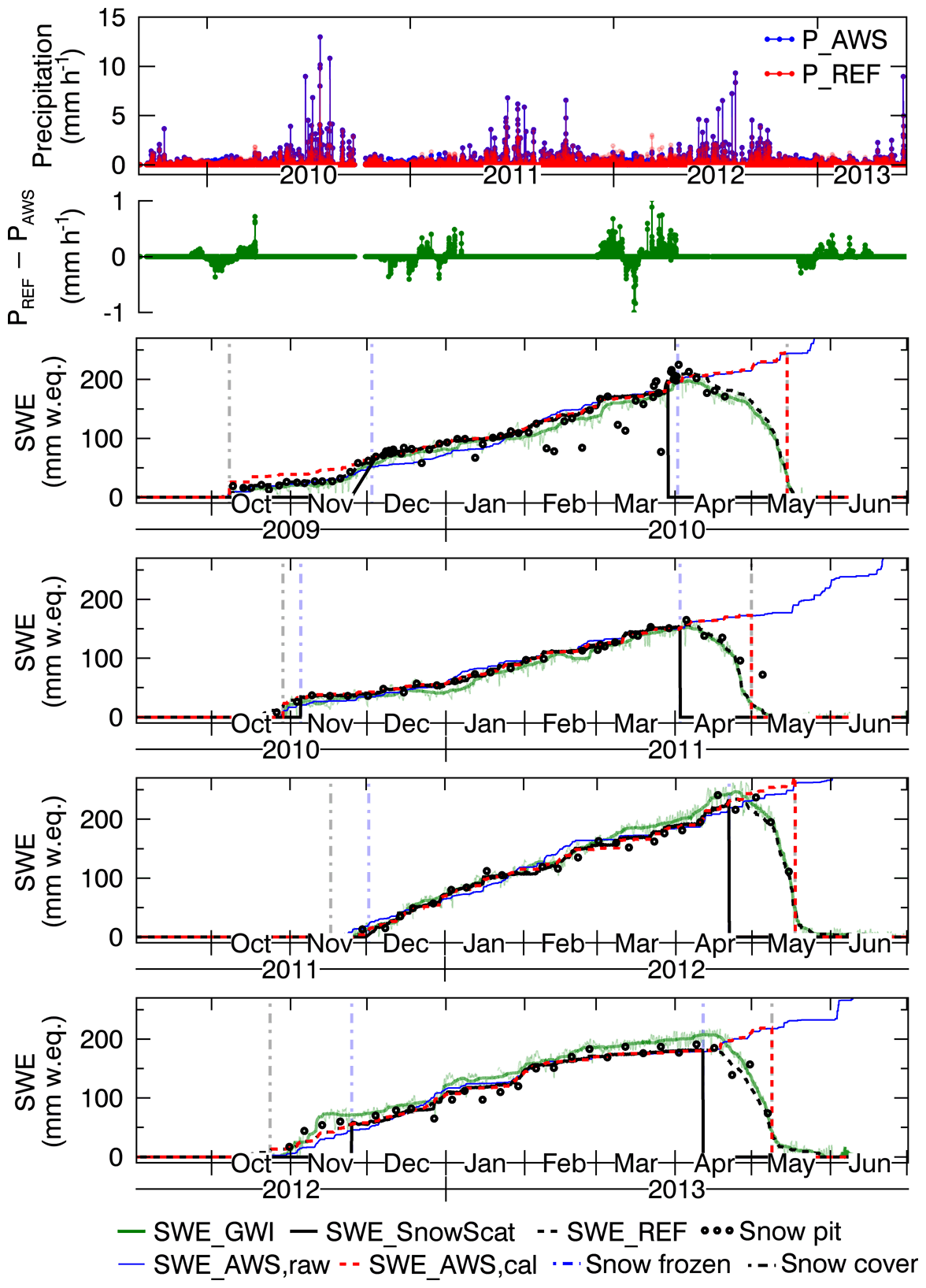
Figure A1Top: precipitation from the AWS, adjusted precipitation (PREF), and difference between both. Below: SWE time series derived from different methods are shown: snow pit data (black bullets), GWI (green), and SnowScat (black). Blue and red lines are the cumulated precipitation of the AWS and the adjusted precipitation PREF. Vertical dashed–dotted lines indicate snow freeze and melt (light blue) and the period of snow-covered ground (gray).
The precipitation phase (PSUM_PH) was measured by the disdrometer located at the IOA (data from https://litdb.fmi.fi, last access: 9 January 2020). However, the data were not directly used because the disdrometer frequently misclassified snow as rain. Therefore, the disdrometer data were only used to check the rain/snow threshold (THRESH_RAIN). According to the disdrometer data combined with air temperature data from the AWS, we determined a rain/snow threshold of T=0.73 ∘C or alternatively a linear range from Tsnow=0.06 to Train=1.40 ∘C (Fig. A2).
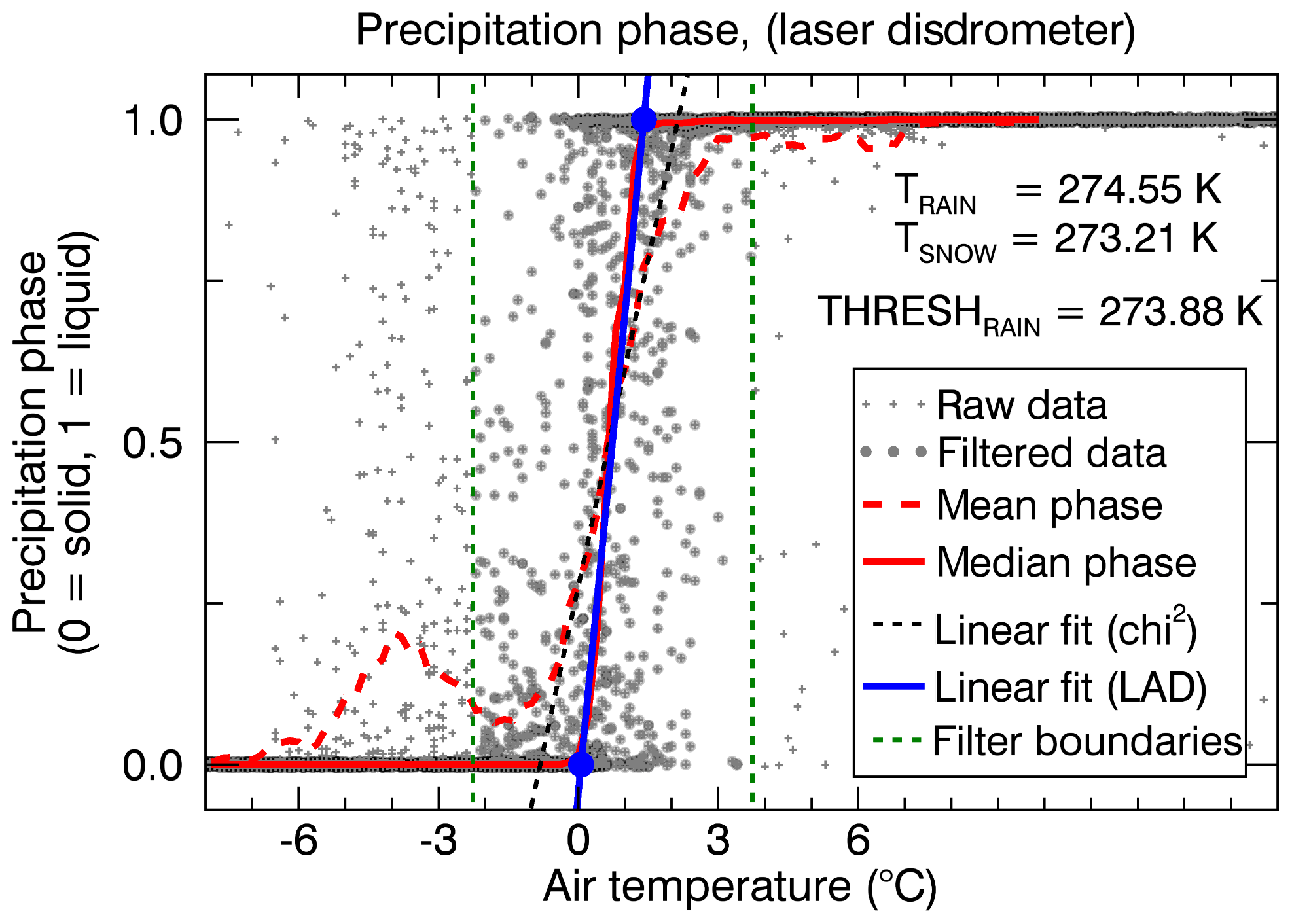
Figure A2From the precipitation phase measured by the disdrometer we determined a mean rain/snow threshold of 0.73 ∘C using a robust least-absolute-deviation (LAD) fit (blue line). A linear fit provides the same threshold but a slightly lower slope. Before fitting, we set a filter boundary (green dotted line) of 0.73±3 ∘C. Data outside the boundary are considered to be misclassified precipitation.
A2 Calibration and interpolation of radiation data
To provide consistent solar radiation data, data acquired by different sensors between January 2009 and September 2015 were homogenized and gaps were interpolated. Plots of the original raw data and the homogenized and filled data are provided in the Figs. S15 (all radiation data), S3–S6 (seasonal raw data), and S7–S10 (seasonal filled data). The incoming shortwave radiation data were almost complete and were interpolated only for a few isolated days. The reflected shortwave radiation data were modeled by SNOWPACK based on the simulated albedo.
The longwave radiation balance was measured at the radiation tower. Longwave radiation data contained a few gaps up to 20 d long (one gap of 52 d in autumn 2011 is irrelevant because this gap is before the onset of snowfall). Data gaps shorter than 12 d were interpolated by the Gaussian average of neighboring data points (FWHM = 1 d, kernel size = 12 d). Remaining gaps of up to 8 d were linearly interpolated. Additionally, to reconstruct the diurnal radiation cycles, the average radiation of each hour of the year was high-pass filtered (Gaussian window of 6 d) and added to the smoothly interpolated data gaps. To provide SNOWPACK the possibility to correctly model snow melting and settling during 21–23 November 2012, the longwave incoming radiation was increased by 45 Wm−2. Webcam observation confirms foggy conditions during this period.
A3 SNOWPACK calibration
For comparison of the natural snowpack with the modeled snowpack under different configuration settings, we compared measured and modeled snow height and snow temperature. Snow temperature was measured at five internal snow temperature sensors at 10, 20, 30, 40, and 50 cm above ground. For snow height and snow temperature we evaluated six statistical descriptors for each of the four seasons: the smallest (negative) difference, the largest (positive) difference, the absolute deviation for which 95 % of all absolute deviations are smaller, the root-mean-square error, the mean difference, and the Nash–Sutcliffe model coefficient. In addition to individual seasons, we calculated these descriptors for the data of all four seasons together. This provided in total quantities for comparisons. To determine the “best” simulation(s), we compared these 60 quantities of every SNOWPACK run with all of the other 5000+ SNOWPACK runs and calculated a score which describes how many times these 60 comparisons show a better result (smaller error, larger Nash–Sutcliffe coefficient) than all other runs. The total score was divided by the total number of runs which results in a score between 0 and 60. A score of 60 indicates that a single run outperforms every other run independent of which statistical variable is analyzed. The maximum achieved score was 51.3, and the lowest score 9.3.
In addition to the relative scoring by pair-wise comparison of all SNOWPACK runs, we used a second scoring scheme which defined fixed height and temperature thresholds for each of the six statistical descriptors. The thresholds are listed in Table A1. The sum of all fulfilled conditions for all years simultaneously and for all individual years again achieved a maximum score of 60. The score by comparison and score by threshold show an approximately linear relation. Histograms over all SNOWPACK runs with the score by threshold and the distribution of statistical descriptors are shown in Fig. S18.
Table A1Thresholds for snow height (HS) and snow temperature (TS) which were used to score the different SNOWPACK runs.
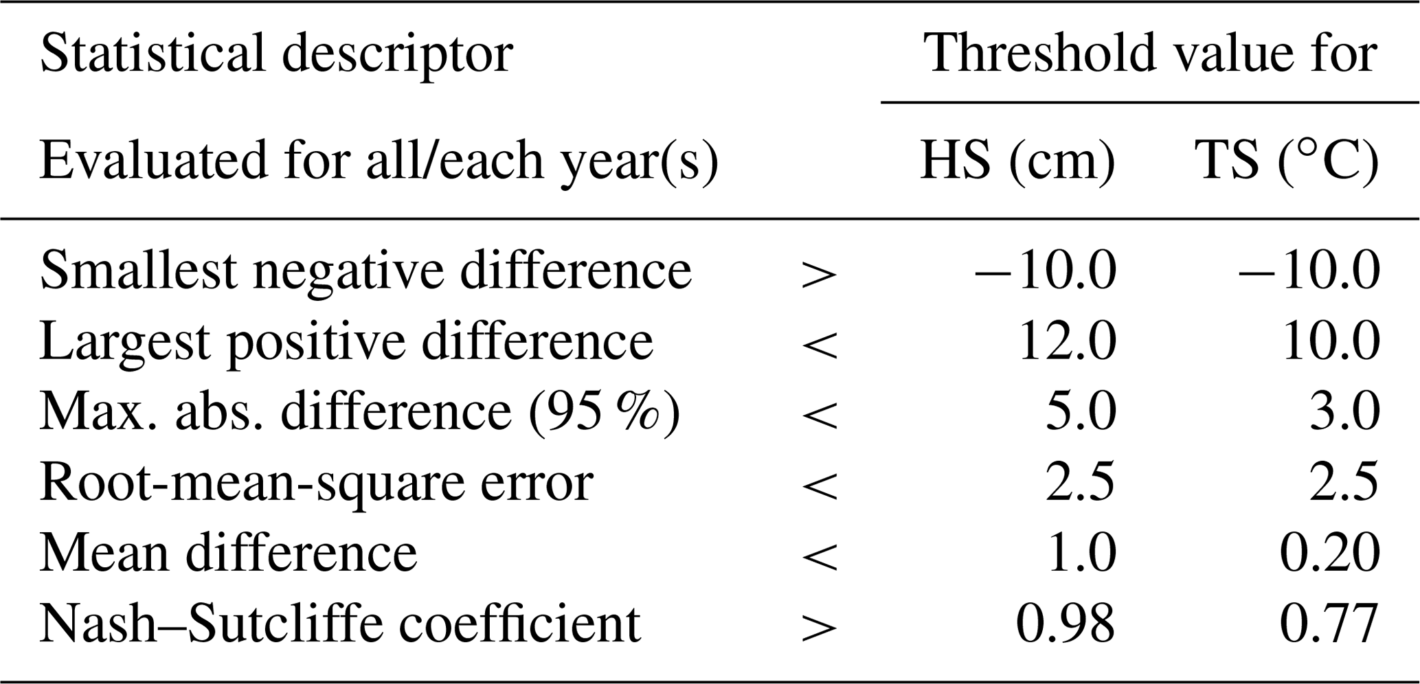
For SNOWPACK calibration, we varied the following parameters: scaling of shortwave and longwave radiation by various constant factors, various thresholds for the snow/rain threshold (THRESH_RAIN), various factors for the WIND_SCALING_FACTOR with SNOW_EROSION = TRUE/FALSE, five different settings for the ATMOSPHERIC_STABILITY, creation of shortwave reflected radiation from albedo (RSWR::create = ISWR_ALBEDO) on/off, calibrated or uncalibrated precipitation PSUM (see Sect. A1), with or without provided precipitation phase (PSUM_PH in *.smet files), filling of longwave radiation gaps with the generator ILWR::allsky_lw::type = Konzelmann or our method described in Sect. A2, and SW_MODE = BOTH/INCOMING.
We found that radiation scaling was crucial to produce correct results. Additionally, snow erosion with a wind scaling factor around 2 significantly improved the results. With atmospheric stability normal we got much better results compared to other atmospheric models. Interestingly, only the model MO_MICHLMAYR required not much modification of the radiation in contrast to the other atmospheric models. Setting SW_MODE = INCOMING instead of BOTH did not change the results except near the end of snowmelt where a slight change was observable. As can be seen, for our test site, SNOWPACK works better when the reflected shortwave radiation is estimated via the albedo than vice versa.
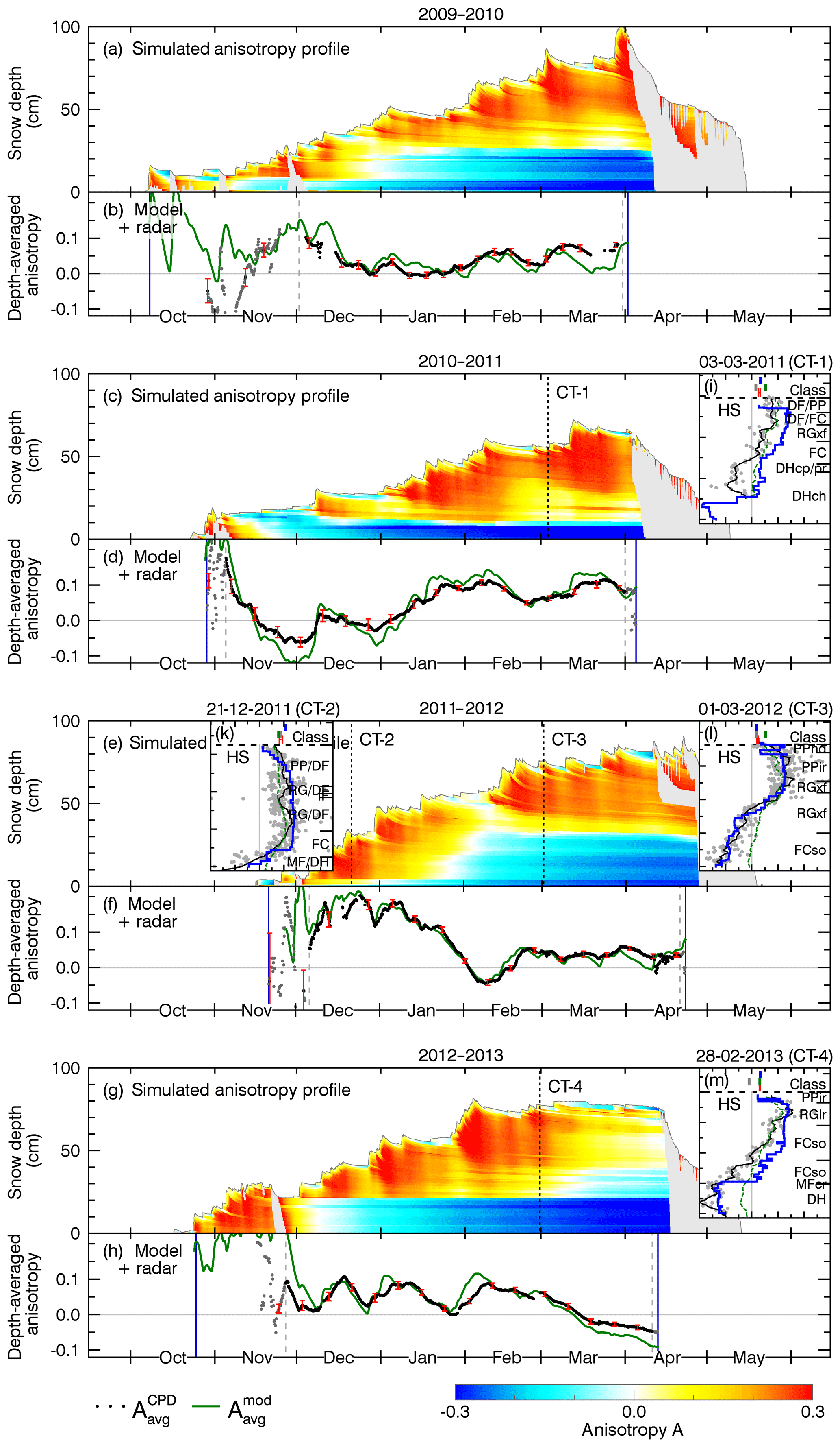
All data are originally from the NoSREx campaigns (Lemmetyinen et al., 2016, 2013) and are partially available from FMI at https://www.litdb.fi, last access: 9 January 2020. Similar, well-calibrated meteorological data are also available from Essery et al. (2016). Radar data are available from ESA or from the GAMMA Remote Sensing and Consulting AG on request. Data of this paper (preprocessed meteorological input data, input and output datasets for SNOWPACK, modeled anisotropy time series, radar-measured CPD and anisotropy time series, SWE measurements and CT data) are available under https://doi.org/10.3929/ethz-b-000382787 (Leinss et al., 2019).
The supplement related to this article is available online at: https://doi.org/10.5194/tc-14-51-2020-supplement.
SL and HL wrote the paper together. SL processed all meteorological and radar data and designed the model. HL processed all CT data. MP, HL, and AK collected the field data.
The authors declare that they have no conflict of interest.
The in situ data collection was supported by the European Space Agency activity “Technical assistance for the deployment of an X- to Ku-band scatterometer during the NoSREx campaigns” (ESA ESTEC contract no. 22671/09/NL/JA/ef) (Lemmetyinen et al., 2013). The staff at FMI-ARC is acknowledged for the collection of in situ data. Andreas Wiesmann from GAMMA Remote Sensing AG is acknowledged for technical assistance with the SnowScat data and Margret Matzl for the lab sampling procedures for casted DEP samples. Special thanks go to Jouni Pulliainen from FMI for the initiative of setting up a test site which provides a unique number and diversity of meteorological data and snow measurements. We thank Matthias Bavey from SLF for helping to find the best SNOWPACK configuration. Juha Lemmetyinen deserves a major thank you for his support concerning all details about the test site and the field data. Irena Hajnsek deserves a major thank you for providing the space and time to write this paper. We thank the editor and the two anonymous reviewers for their time and their constructive comments. The paper was funded by ETH Zürich.
This paper was edited by Guillaume Chambon and reviewed by two anonymous referees.
Alley, R. B.: Texture of polar firn for remote sensing, Ann. Glaciol., 9, 1–4, https://doi.org/10.3189/S0260305500200670, 1987. a, b
Bartelt, P. and Lehning, M.: A physical SNOWPACK model for the Swiss avalanche warning: Part I: numerical model, Cold Reg. Sci. Technol., 35, 123–145, https://doi.org/10.1016/S0165-232X(02)00074-5, 2002. a, b, c
Brun, E., Martin, E., Simon, V., Gendre, C., and Coleou, C.: An energy and mass model of snow cover suitable for operational avalanche forecasting, J. Glaciol., 35, 333–342, https://doi.org/10.3189/S0022143000009254, 1989. a
Brun, E., David, P., Sudul, M., and Brunot, G.: A numerical model to simulate snow-cover stratigraphy for operational avalanche forecasting, J. Glaciol., 38, 13–22, https://doi.org/10.3189/S0022143000009552, 1992. a, b
Calonne, N., Flin, F., Morin, S., Lesaffre, B., du Rolland du Roscoat, S., and Geindreau, C.: Numerical and experimental investigations of the effective thermal conductivity of snow, Geophys. Res. Lett., 38, 1–6, https://doi.org/10.1029/2011GL049234, 2011. a
Calonne, N., Geindreau, C., Flin, F., Morin, S., Lesaffre, B., Rolland du Roscoat, S., and Charrier, P.: 3-D image-based numerical computations of snow permeability: links to specific surface area, density, and microstructural anisotropy, The Cryosphere, 6, 939–951, https://doi.org/10.5194/tc-6-939-2012, 2012. a
Calonne, N., Flin, F., Geindreau, C., Lesaffre, B., and Rolland du Roscoat, S.: Study of a temperature gradient metamorphism of snow from 3-D images: time evolution of microstructures, physical properties and their associated anisotropy, The Cryosphere, 8, 2255–2274, https://doi.org/10.5194/tc-8-2255-2014, 2014. a, b, c, d, e, f
Calonne, N., Montagnat, M., Matzl, M., and Schneebeli, M.: The layered evolution of fabric and microstructure of snow at Point Barnola, Central East Antarctica, Earth Planet. Sc. Lett., 460, 293–301, https://doi.org/10.1016/j.epsl.2016.11.041, 2016. a
Chang, P., Mead, J., Knapp, E., Sadowy, G., Davis, R., and McIntosh, R.: Polarimetric backscatter from fresh and metamorphic snowcover at millimeter wavelengths, IEEE T. Antennas Propag., 44, 58–73, https://doi.org/10.1109/8.477529, 1996. a
Colbeck, S. C.: The vapor diffusion coefficient for snow, Water Resour. Res., 29, 109–115, https://doi.org/10.1029/92WR02301, 1993. a
Davis, R. E. and Dozier, J.: Stereological characterization of dry Alpine snow for microwave remote sensing, Adv. Space Res., 9, 245–251, https://doi.org/10.1016/0273-1177(89)90492-4, 1989. a
Essery, R., Kontu, A., Lemmetyinen, J., Dumont, M., and Ménard, C. B.: A 7-year dataset for driving and evaluating snow models at an Arctic site (Sodankylä, Finland), Geosci. Instrum. Method. Data Syst., 5, 219–227, https://doi.org/10.5194/gi-5-219-2016, 2016. a, b, c
Fierz, C., Armstrong, R., Durand, Y., Etchevers, P., Greene, E., McClung, D., Nishimura, K., Satyawali, P., and Sokratov, S.: The International Classification for Seasonal Snow on the Ground. IHP-VII Technical Documents in Hydrology No. 83, IACS Contribution No. 1, UNESCO-IHP, Paris, 90 pp., 2009. a
Fujita, S., Okuyama, J., Hori, A., and Hondoh, T.: Metamorphism of stratified firn at Dome Fuji, Antarctica: A mechanism for local insolation modulation of gas transport conditions during bubble close off, J. Geophys. Res.-Earth, 114, 1–21, https://doi.org/10.1029/2008JF001143, 2009. a, b
Heggli, M., Frei, E., and Schneebeli, M.: Snow replica method for three-dimensional X-ray microtomographic imaging, J. Glaciol., 55, 631–639, https://doi.org/10.3189/002214309789470932, 2009. a
Izumi, K. and Huzioka, T.: Studies of metamorphism and thermal conductivity of snow, 1. Low temperature science, Series A, Phys. Sci., 33, 91–102, 1975. a
Jordan, R.: A one-dimensional temperature model for a snow cover: Technical documentation for SNTHERM, 89, Tech. Rep., US Army Cold Regions Research and Engineering Laboratory, Hanover NH, Special Report 91-16, 64 pp., 1991. a
Kaempfer, T. U., Schneebeli, M., and Sokratov, S. A.: A microstructural approach to model heat transfer in snow, Geophys. Res. Lett., 32, 1–5, https://doi.org/10.1029/2005GL023873, l21503, 2005. a
Krol, Q. and Löwe, H.: Relating optical and microwave grain metrics of snow: the relevance of grain shape, The Cryosphere, 10, 2847–2863, https://doi.org/10.5194/tc-10-2847-2016, 2016. a
Lamb, D. and Hobbs, P. V.: Growth rates and habits of ice crystals grown from the vapor phase, J. Atmos. Sci., 28, 1506–1509, https://doi.org/10.1021/j100244a032, 1971. a
Lamb, D. and Scott, W. D.: Linear growth rates of ice crystals grown from the vapor phase, J. Cryst. Growth, 12, 21–31, https://doi.org/10.1016/0022-0248(72)90333-8, 1972. a
Lehning, M., Bartelt, P., Brown, B., and Fierz, C.: A physical SNOWPACK model for the Swiss avalanche warning: Part III: meteorological forcing, thin layer formation and evaluation, Cold Reg. Sci. Technol., 35, 169–184, https://doi.org/10.1016/S0165-232X(02)00072-1, 2002a. a, b
Lehning, M., Bartelt, P., Brown, B., Fierz, C., and Satyawali, P.: A physical SNOWPACK model for the Swiss avalanche warning: Part II. Snow microstructure, Cold Reg. Sci. Technol., 35, 147–167, https://doi.org/10.1016/S0165-232X(02)00073-3, 2002b. a, b
Leinss, S., Parrella, G., and Hajnsek, I.: Snow height determination by polarimetric phase differences in X-band SAR data, IEEE J. Sel. Topics Appl. Earth Observ. Remote Sens., 7, 3794–3810, https://doi.org/10.1109/JSTARS.2014.2323199, 2014. a, b, c
Leinss, S., Wiesmann, A., Lemmetyinen, J., and Hajnsek, I.: Snow water equivalent of dry snow measured by differential interferometry, IEEE J. Sel. Topics Appl. Earth Observ. Remote Sens., 8, 3773–3790, https://doi.org/10.1109/JSTARS.2015.2432031, 2015. a, b
Leinss, S., Löwe, H., Proksch, M., Lemmetyinen, J., Wiesmann, A., and Hajnsek, I.: Anisotropy of seasonal snow measured by polarimetric phase differences in radar time series, The Cryosphere, 10, 1771–1797, https://doi.org/10.5194/tc-10-1771-2016, 2016. a, b, c, d, e, f, g, h, i, j, k, l, m, n, o, p
Leinss, S., Löwe, H., Proksch, M., and Kontu, A.: Modeling the Evolution of the Structural Anisotropy of Snow, https://doi.org/10.3929/ethz-b-000382787, 2019. a
Lemmetyinen, J., Kontu, A., Leppänen, L., Pulliainen, J., Wiesmann, A., Werner, C., Proksch, M., and Schneebeli, M.: Technical assistance for the deployment of an X- to Ku-band scatterometer during the NoSREx experiment, NoSREx-I, -II and -III (2009–2012) Final report, Contract No. 22671/09/NL/JA/ef, Tech. Rep., ESA ESTEC, Noordwijk, available at: https://earth.esa.int/web/guest/campaigns (last access: 9 January 2020), 2013. a, b, c, d, e
Lemmetyinen, J., Kontu, A., Pulliainen, J., Vehviläinen, J., Rautiainen, K., Wiesmann, A., Mätzler, C., Werner, C., Rott, H., Nagler, T., Schneebeli, M., Proksch, M., Schüttemeyer, D., Kern, M., and Davidson, M. W. J.: Nordic Snow Radar Experiment, Geosci. Instrum. Method. Data Syst., 5, 403–415, https://doi.org/10.5194/gi-5-403-2016, 2016. a, b, c
Leppänen, L., Kontu, A., Vehviläinen, J., Lemmetyinen, J., and Pulliainen, J.: Comparison of traditional and optical grain-size field measurements with SNOWPACK simulations in a taiga snowpack, J. Glaciol., 61, 151–162, https://doi.org/10.3189/2015JoG14J026, 2015. a
Libbrecht, K. G.: The physics of snow crystals, Rep. Prog. Phys., 68, 855–895, https://doi.org/10.1088/0034-4885/68/4/r03, 2005. a
Löwe, H., Spiegel, J. K., and Schneebeli, M.: Interfacial and structural relaxations of snow under isothermal conditions, J. Glaciol., 57, 499–510, https://doi.org/10.3189/002214311796905569, 2011. a, b, c, d
Löwe, H., Riche, F., and Schneebeli, M.: A general treatment of snow microstructure exemplified by an improved relation for thermal conductivity, The Cryosphere, 7, 1473–1480, https://doi.org/10.5194/tc-7-1473-2013, 2013. a, b, c, d, e
Marti, J. and Mauersberger, K.: A survey and new measurements of ice vapor pressure at temperatures between 170 and 250 K, Geophys. Res. Lett., 20, 363–366, https://doi.org/10.1029/93GL00105, 1993. a
Massman, W. J.: A review of the molecular diffusivities of H2O, CO2, CH4, CO, O3, SO2, NH3, N2O, NO, and NO2 in air, O2 and N2 near STP, Atmos. Environ., 32, 1111–1127, https://doi.org/10.1016/S1352-2310(97)00391-9, 1998. a
Mätzler, C.: Applications of the interaction of microwaves with the natural snow cover, Remote Sens. Rev., 2, 259–387, https://doi.org/10.1080/02757258709532086, 1987. a
Mätzler, C.: Autocorrelation functions of granular media with free arrangement of spheres, spherical shells or ellipsoids, J. Appl. Phys., 81, 1509–1517, https://doi.org/10.1063/1.363916, 1997. a
Mätzler, C.: Relation between grain-size and correlation length of snow, J. Glaciol., 48, 461–466, https://doi.org/10.3189/172756502781831287, 2002. a, b, c, d
Miller, D. A. and Adams, E. E.: A microstructural dry-snow metamorphism model for kinetic crystal growth, J. Glaciol., 55, 1003–1011, https://doi.org/10.3189/002214309790794832, 2009. a
Pinzer, B. R. and Schneebeli, M.: Snow metamorphism under alternating temperature gradients: Morphology and recrystallization in surface snow, Geophys. Res. Lett., 36, 1–4, https://doi.org/10.1029/2009GL039618, 2009. a
Pinzer, B. R., Schneebeli, M., and Kaempfer, T. U.: Vapor flux and recrystallization during dry snow metamorphism under a steady temperature gradient as observed by time-lapse micro-tomography, The Cryosphere, 6, 1141–1155, https://doi.org/10.5194/tc-6-1141-2012, 2012. a, b, c, d, e
Proksch, M., Löwe, H., and Schneebeli, M.: Density, specific surface area and correlation length of snow measured by high-resolution penetrometry, J. Geophys. Res.-Earth, 120, 346–362, https://doi.org/10.1002/2014JF003266, 2015. a
Rechtsman, M. C. and Torquato, S.: Effective dielectric tensor for electromagnetic wave propagation in random media, J. Appl. Phys., 103, 084901, https://doi.org/10.1063/1.2906135, 2008. a
Riche, F. and Schneebeli, M.: Thermal conductivity of snow measured by three independent methods and anisotropy considerations, The Cryosphere, 7, 217–227, https://doi.org/10.5194/tc-7-217-2013, 2013. a
Riche, F., Montagnat, M., and Schneebeli, M.: Evolution of crystal orientation in snow during temperature gradient metamorphism, J. Glaciol., 59, 47–55, https://doi.org/10.3189/2013JoG12J116, 2013. a, b, c
Schleef, S. and Löwe, H.: X-ray microtomography analysis of isothermal densification of new snow under external mechanical stress, J. Glaciol., 59, 233–243, https://doi.org/10.3189/2013JoG12J076, 2013. a, b
Schleef, S., Löwe, H., and Schneebeli, M.: Hot-pressure sintering of low-density snow analyzed by X-ray microtomography and in situ microcompression, Acta Mater., 71, 185–194, https://doi.org/10.1016/j.actamat.2014.03.004, 2014. a
Schneebeli, M. and Sokratov, S.: Tomography of temperature gradient metamorphism of snow and associated changes in heat conductivity, Hydrol. Process., 18, 3655–3665, https://doi.org/10.1002/hyp.5800, 2004. a, b, c
Shertzer, R. H. and Adams, E. E.: Anisotropic thermal conductivity model for dry snow, Cold Reg. Sci. Technol., 69, 122–128, https://doi.org/10.1016/j.coldregions.2011.09.005, 2011. a, b
Sokratov, S. A. and Maeno, N.: Effective water vapor diffusion coefficient of snow under a temperature gradient, Water Resour. Res., 36, 1269–1276, https://doi.org/10.1029/2000WR900014, 2000. a
Srivastava, P. K., Mahajan, P., Satyawali, P. K., and Kumar, V.: Observation of temperature gradient metamorphism in snow by X-ray computed microtomography: measurement of microstructure parameters and simulation of linear elastic properties, Ann. Glaciol., 51, 73–82, https://doi.org/10.3189/172756410791386571, 2010. a
Srivastava, P. K., Chandel, C., Mahajan, P., and Pankaj, P.: Prediction of anisotropic elastic properties of snow from its microstructure, Cold Reg. Sci. Technol., 125, 85–100, https://doi.org/10.1016/j.coldregions.2016.02.002, 2016. a, b
Staron, P. J., Adams, E. E., and Miller, D. A.: Nonequilibrium thermodynamics of kinetic metamorphism in snow, Cold Reg. Sci. Technol., 97, 60–71, https://doi.org/10.1016/j.coldregions.2013.10.007, 2014. a
Sturm, M., Holmgren, J., König, M., and Morris, K.: The thermal conductivity of seasonal snow, J. Glaciol., 43, 26–41, https://doi.org/10.3189/S0022143000002781, 1997. a
ToolBox, E.: Thermal conductivity of common materials and gases, available at: https://www.engineeringtoolbox.com/thermal-conductivity-d_429.html (last access: 9 January 2020), 2003a. a
ToolBox, E.: Specific heat of common substances, available at: https://www.engineeringtoolbox.com/specific-heat-capacity-d_391.html (last access: 9 January 2020), 2003b. a
Torquato, S.: Random heterogeneous materials, Springer, New York, 2002. a
Torquato, S. and Lado, F.: Trapping constant, thermal conductivity, and the microstructure of suspensions of oriented spheroids, J. Chem. Phys., 94, 4453–4462, https://doi.org/10.1063/1.460635, 1991. a
Vallese, F. and Kong, J. A.: Correlation function studies for snow and ice, J. Appl. Phys., 52, 4921–4925, https://doi.org/10.1063/1.329453, 1981. a
Werner, C., Wiesmann, A., Strozzi, T., Schneebeli, M., and Mätzler, C.: The SnowScat ground-based polarimetric scatterometer: Calibration and initial measurements from Davos Switzerland, in: IEEE International Geoscience and Remote Sensing Symposium (IGARSS 2010), 25–30 July 2010, Honolulu, Hawaii, USA, 2363–2366, https://doi.org/10.1109/IGARSS.2010.5649015, 2010. a
Wiese, M. and Schneebeli, M.: Early-stage interaction between settlement and temperature-gradient metamorphism, J. Glaciol., 63, 652–662, https://doi.org/10.1017/jog.2017.31, 2017. a, b, c, d, e
Yosida, Z.: Physical studies on deposited snow, I. Thermal properties, Contributions from the Institute of Low Temperature Science, 7, 19–74, available at: http://hdl.handle.net/2115/20216 (last access: 9 January 2020), 1955. a, b
Zermatten, E., Haussener, S., Schneebeli, M., and Steinfeld, A.: Tomography-based determination of permeability and Dupuit-Forchheimer coefficient of characteristic snow samples, J. Glaciol., 57, 811–816, https://doi.org/10.3189/002214311798043799, 2011. a
- Abstract
- Introduction
- A dynamical model for the structural anisotropy
- Datasets and methods
- Results
- Discussion
- Conclusions
- Appendix A: Preprocessing of meteorological data and SNOWPACK calibration
- Data availability
- Author contributions
- Competing interests
- Acknowledgements
- Review statement
- References
- Supplement