2.1 Study area

Fountain Glacier, located on Bylot Island, Nunavut (Fig. 1), has been studied in detail since 1991 (e.g. Moorman, 2003; Whitehead et al., 2014; Bash et al., 2018). The glacier stretches across 16 km, from higher elevations in the Byam Martin Mountain Range to its terminus roughly 10 km inland from the coast. The focus area of this study, in the lower ablation zone, spans a narrow elevation range (250–400 m) and terminates in a cliff face with two calving fronts. The lower portion of the glacier faces east, with several supraglacial streams of varying sizes (St. Germain and Moorman, 2016). The largest of these streams form deeply incised asymmetrical canyons, with a steeper north-facing valley wall and a more gently sloping south-facing valley wall (Fig. 1).

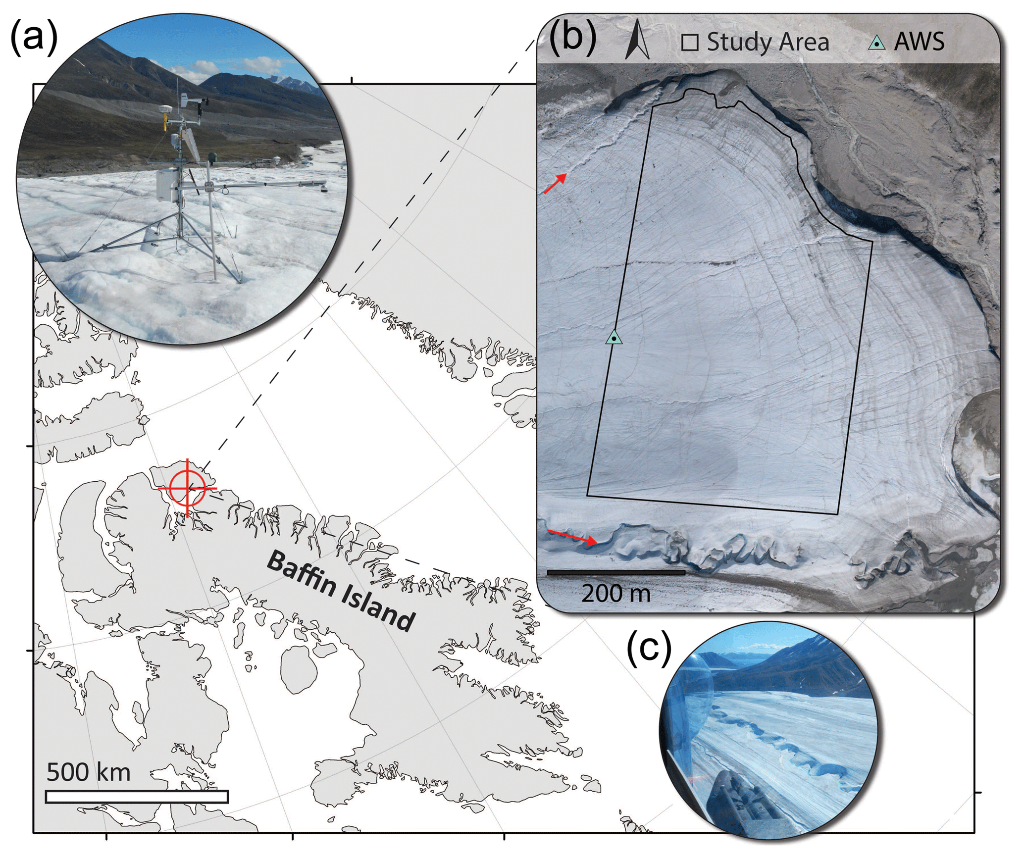
Figure 1Location of Fountain Glacier on Bylot Island, Nunavut, in the Canadian Arctic. (a) The automatic weather station (AWS) installed on a tripod, measuring incoming and outgoing shortwave radiation and temperature. An SR50 measuring surface position was installed on a separate pole drilled into the glacier (foreground; photo credit: E. A. Bash). (b) A 2011 orthomosaic of the lower ablation zone of Fountain Glacier (Whitehead et al., 2013). The boundary of the study area is shown, which extends to the 2016 glacier boundary on the north side. The AWS location is also indicated (green triangle). Two canyons formed by stream incision are indicated by red arrows. (c) An aerial view of the largest incised canyon on Fountain Glacier. The photo is taken facing east, and the steep north-facing canyon walls can be seen in contrast to the more gently sloping south-facing walls (photo credit: B. J. Moorman).

During July 2016 aerial surveys were conducted with a UAV to reconstruct 0.185 km² of the glacier surface multiple times (Bash et al., 2018). Bash et al. (2018) measured surface lowering between 21 and 24 July using point cloud differencing across the study area indicated in Fig. 1. Concurrently, an AWS (Fig. 1) recorded surface melt with a Campbell Scientific SR50 sonic ranger as well as temperature, incoming and outgoing shortwave radiation, relative humidity, wind speed, and direction. Bash et al. (2018) assessed the surface lowering measured through point cloud differencing against 17 ablation stakes, as well as the AWS data, and found that the measured surface lowering agreed with other melt measurements throughout the study area. In this study we assume that surface lowering derived from point clouds is equivalent to surface melt. The uncertainty of this surface lowering was 0.048 m.

Bash et al. (2018) measured an average daily melt rate of 0.060 m d⁻¹ across the study area between 21 and 24 July 2016. Between 2010 and 2011, Whitehead et al. (2014) measured melt rates of 0.030–0.055 m d⁻¹ across the ablation zone. Bash et al. (2018) also showed, however, that melt was highly variable across the study area during July 2016, ranging from 0.010 to 0.110 m d⁻¹. The authors found that these differences in melt were not tied to the elevation or aspect of the glacier surface.

2.2 Description of data

All AWS measurements were taken at 2 min intervals and recorded as hourly averages from 1 to 31 July 2016 (Fig. 2). The SR50 was installed on a pole drilled into the glacier surface immediately next to the AWS on 13 July and measured hourly average surface height. The pole holding the SR50 began to tilt due to melt out of the pole during the afternoon of 27 July and was reinstalled in the morning on 28 July. The data from that time period were removed from the time series for model validation.

Figure 2Hourly averaged melt model input variables, measured at the AWS for the period 1–31 July 2016. Variables include near-surface air temperature (a), incoming (SW_in) and outgoing (SW_out) shortwave radiation (b), albedo (c), wind speed (d), and relative humidity (e). Inputs which are estimated for distributed models are shown in red for incoming shortwave radiation (a) and albedo (b). The albedo derived from UAV imagery is scaled using the average value at the AWS for 21–24 July so that it remains constant throughout the model. The dates of the UAV study are shown in grey.

Download

Models run at high temporal resolution can have significant errors which stem from SR50 readings (Matthews et al., 2015). These errors stem from the uncertainty in SR50 readings due to the instrument accuracy (0.01 m) as well as uneven topography underneath the instrument. In addition to hourly surface height, the SR50 records a standard deviation of all measurements in the hourly average (typically 30 measurements). SR50 values where the standard deviation was greater than 0.01 m were removed, expected hourly melt rates are lower than the instrument accuracy, and standard deviations greater than that are assumed to be related to noise. After removing those points, a 5 h rolling average was calculated to smooth the data and fill in removed values. The 5 h window was used to assure that all windows had multiple measurements to average after some measurements had been removed. SR50 values which differed significantly from others in the 5 h window were also removed (defined as more than the standard deviation of hourly change in the 5 h window) under an assumption that it was physically unlikely for melt rates to change dramatically over short periods. Melt was then calculated in 12 h periods (00:00–12:00 LT) using the remaining values.

Processing of UAV imagery was done in Agisoft PhotoScan and is described in detail by Bash et al. (2018). High-accuracy settings were used to retain detail in the final point cloud. During processing, point clouds of the glacier surface at midday were produced for 21 and 24 July 2016. The point clouds were used to create orthomosaics and digital surface models (DSMs) for each day with horizontal resolutions of 0.10 m.

The multiscale model to model cloud comparison (M3C2) was used to calculate melt across the study area at 0.02 m horizontal resolution (Lague et al., 2013; Bash et al., 2018), with vertical uncertainty of 0.048 m based on the root-mean-square error (RMSE) of surface lowering compared to ablation stakes. The M3C2 algorithm calculates change normal to the local surface, which was desirable for measuring detailed change at such fine resolution. After differencing the point clouds were filtered to remove large outliers and differences calculated from fewer than five points, as suggested by Lague et al. (2013). This filtering resulted in variable density of points in the final point cloud. To align with DSMs and orthomosaics of the study area, for this study melt data were gridded to 0.10 m resolution. Melt measurements were averaged within each grid cell, and empty cells were filled using bilinear interpolation.

2.3 Model formulation

2.3.1 Energy balance model

An EB model accounts for all energy inputs and outputs at the glacier surface to estimate energy available for melt or freezing. As a representation of surface energy exchange, these models are often assumed to be the best estimators of surface melt (Hock, 2005). We employ an energy balance model described by Ebrahimi and Marshall (2016) as a check on both SfM-derived change and the ETI model described below:

$$\begin{array}{}\text{(1)}& Q_{\mathrm{N}}=Q_{\mathrm{SW}}^{\downarrow }-Q_{\mathrm{SW}}^{\uparrow }+Q_{\mathrm{L}}^{\downarrow }-Q_{\mathrm{L}}^{\uparrow }+Q_{\mathrm{H}}+Q_{\mathrm{E}},\end{array}$$

where Q_N is the net energy flux at the surface and $Q_{\mathrm{SW}}^{\downarrow }$, $Q_{\mathrm{SW}}^{\uparrow }$, $Q_{\mathrm{L}}^{\downarrow }$, $Q_{\mathrm{L}}^{\uparrow }$, Q_H, and Q_E represent incoming and outgoing shortwave radiation, incoming and outgoing longwave radiation, and sensible and latent heat flux, respectively. The energy fluxes are all calculated in megajoules per square meter per hour (MJ m⁻² h⁻¹). For consistency with AWS measurements, and energy fluxes are positive when they contribute energy to the glacier surface. When Q_N>0 melt ($\widehat{M}$; m ice) is calculated by

$$\begin{array}{}\text{(2)}& \widehat{M}={\displaystyle \frac{Q_{\mathrm{N}}}{{\mathit{\rho }}_{\mathrm{ice}}{L}_{\mathrm{f}}}},\end{array}$$

where ρ_ice is the density of glacier ice, assumed to be 900 kg m³ (e.g. Arnold et al., 2006; Cuffey and Paterson, 2010; Fitzpatrick et al., 2017), and L_f is the latent heat of fusion. Longwave radiation (Q_L) is parameterised based on the absolute temperature (T) and emissivity (ε):

$$\begin{array}{}\text{(3)}& Q_{\mathrm{L}}=\mathit{\epsilon }\mathit{\delta }{T}^{\mathrm{4}},\end{array}$$

where δ is the Stefan–Boltzmann constant. For $Q_{\mathrm{L}}^{\uparrow }$, the calculation is straightforward if the surface is assumed to be melting (273.15 K); the surface emissivity is then 1.0. The atmospheric emissivity (ε_a) must be estimated in order to obtain $Q_{\mathrm{L}}^{\downarrow }$. Here we use a parameterisation from Ebrahimi and Marshall (2015) based on vapour pressure (e_v) and relative humidity (H), which was found to be robust when transferred directly without local training:

$$\begin{array}{}\text{(4)}& {\mathit{\epsilon }}_{\mathrm{a}}=\mathrm{0.445}+\mathrm{0.0055}H+\mathrm{0.0052}{e}_{\mathrm{v}}.\end{array}$$

The sensible and latent heat fluxes are calculated by Eqs. (5) and (7), respectively:

$$\begin{array}{}\text{(5)}& Q_{\mathrm{H}}={\mathit{\rho }}_{\mathrm{a}}{c}_{\mathrm{p}}{k}^{\mathrm{2}}v\left[{\displaystyle \frac{T_{\mathrm{pa}}-T_{\mathrm{ps}}}{\ln \left(z/z_{\mathrm{0}}\right)\ln \left(z/z_{\mathrm{0}\mathrm{H}}\right)}}\right],\end{array}$$

where ρ_a is the air density, calculated from the near-surface air temperature and average air pressure at the AWS (P_aws=969), c_p is the heat capacity of air, v is the measured wind speed, and k=0.4 is von Karman's constant. The potential temperature is calculated for the near-surface air (T_pa) and ice surface by (T_ps)

$$\begin{array}{}\text{(6)}& T_{\mathrm{p}}=T{{\displaystyle \frac{P_{\mathrm{ref}}}{P_{\mathrm{aws}}}}}^{R/c_{\mathrm{p}}},\end{array}$$

where P_ref is a reference pressure (1000 mbar), R=288.5, and the surface is assumed to be at the melting point.

$$\begin{array}{}\text{(7)}& Q_{\mathrm{E}}={\mathit{\rho }}_{\mathrm{a}}{L}_{\mathrm{v}}{k}^{\mathrm{2}}v\left[{\displaystyle \frac{q_{\mathrm{a}}-q_{\mathrm{s}}}{\ln \left(z/z_{\mathrm{0}}\right)\ln \left(z/z_{\mathrm{0}\mathrm{E}}\right)}}\right],\end{array}$$

where L_v is the latent heat of vaporisation, q_a is the specific humidity, based on T and H, and q_s is the specific humidity calculated from the saturation vapour pressure at the melting surface. z₀, z_0H, and z_0E are the roughness length scales for turbulent exchange of momentum, heat, and moisture. The height of all AWS measurements is z=1.5 m, and z₀=0.005 m was used as a tuning parameter at the AWS. Both Eqs. (5) and (7) neglect a correction for atmospheric stability, which has been shown in previous studies to provide better results for these parameters (Hock and Holmgren, 2005; Ebrahimi and Marshall, 2016).

A 1-D formulation of this model (EB_aws) runs using measured inputs from the AWS. A distributed version was also developed (EB_dist) using modelled incoming radiation at the AWS location and albedo derived from the UAV imagery to determine SW_net (both described below; Figs. 2b and c and 3). Near-surface air temperature across the study area was modelled using the uncorrelated AWS temperature and modelled radiation (Sect. 2.3.2). Measured values from the AWS are used for all other variables in Eqs. (3)–(7).

Distributed surface albedo

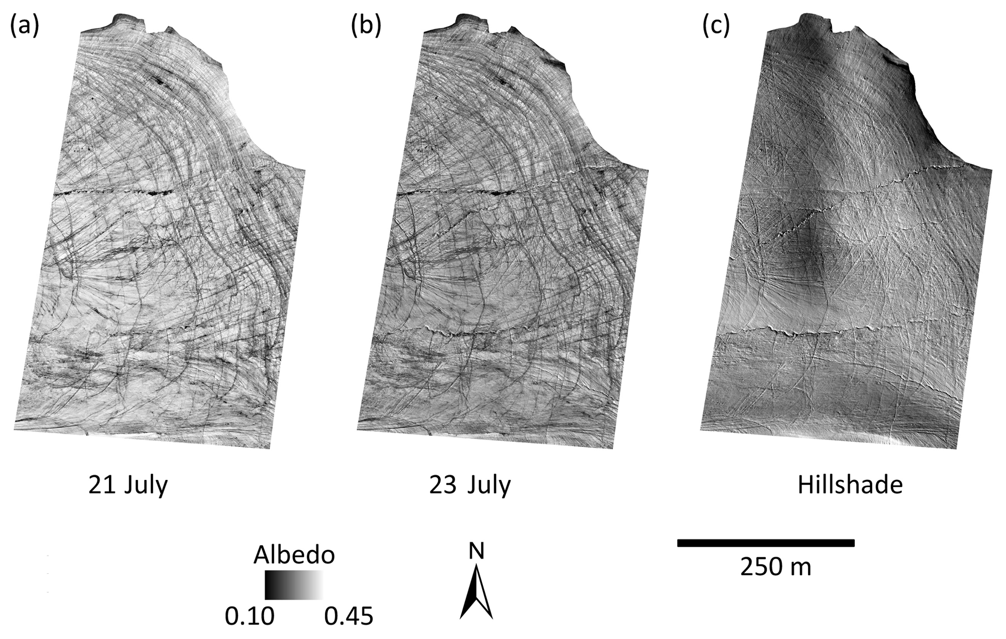
Figure 3Albedo was derived from UAV imagery using average values from RGB bands and scaling the lower and upper bounds to match the albedo of bare rocks (based on Ryan et al., 2017) and the average albedo measured on Fountain Glacier during the study period. (a) 21 July albedo values. (b) 23 July albedo values. (c) A hillshade model of the study area based on the DSM from 21 July.

Download

Distributed incoming radiation was modelled by modifying the hourly measured incoming radiation at the AWS by the slope (S) and aspect (A) of each grid cell in the 21 July DSM (Fig. 3c). The terrain correction was based on Goswami et al. (2000):

$$\begin{array}{}\text{(8)}& {\mathrm{SW}}_{\mathrm{in}}=Q_{\mathrm{SW}}^{\downarrow }\cdot \cos \mathit{\psi }\cdot \cos (\mathit{\omega }-A)\cdot \sin S\cdot \cos S,\end{array}$$

where ψ is the solar altitude and ω the solar azimuth. This correction alone causes radiation to drop to zero overnight, which is not realistic during Arctic summers. Although direct radiation may drop to zero at some cells when sun angles are low overnight (solar elevation dips to 3.6^∘), diffuse radiation is at measurable levels (Fig. 2b). A diffuse correction (SW_diff; based on Bugler, 1977) was added to incoming radiation after correction for the incidence angle to estimate the total incoming radiation (Fig. 2b):

$$\begin{array}{}\text{(9)}& {\mathrm{SW}}_{\mathrm{diff}}=\mathrm{16}{\mathit{\psi }}^{\mathrm{0.5}}-\mathrm{0.4}\mathit{\psi }.\end{array}$$

Lower peak radiation in the model (Fig. 2b) is due to a slight difference in slope and aspect between the radiometer (which was level) and the grid cell of the DSM containing the AWS (slope = 5^∘; aspect = 177^∘). Estimated radiation at each cell was then multiplied by (1−α) to estimate SW_net at each cell.

Albedo was estimated across the study area using the orthomosaics from 21 and 23 July. Each orthomosaic contains the digital number recorded by the camera in the red, green, and blue (RGB) channels. The digital number cannot be directly used to calculate surface reflectance without conversion equations proprietary to the camera manufacturer. However, several studies have used other approaches to derive surface reflectance from digital numbers (Corripio, 2004; Rippin et al., 2015; Ryan et al., 2017). Rippin et al. (2015) use the sum of RGB digital number values as a proxy for albedo, similar to the approach we employ here.

Values for RGB channels were averaged and the total range scaled to match the value at the AWS location (Fig. 3). Scaling in this way allows the values to be directly input into models, as opposed to providing a proxy for albedo, as was done in Rippin et al. (2015). The average measured albedo value for the study period (0.31; 21–24 July 2016) was used to fix the rescaled value for both 21 and 23 July at the AWS location. The lower end of the range was based on albedo values of cryoconite holes reported by Ryan et al. (0.1; 2017); an assumption was made that cryoconite holes would have similar albedo to debris on the glacier surface. The scaling of RGB values was used to create two gridded albedo products that could be directly input into the melt model (Fig. 3); on 21 July albedo was used as a model input up until 12:00 LT on 23 July, while the 23 July albedo was used from 12:00 LT on 23 July onward.

Mean albedo over the grid was 0.35 for 21 July and 0.33 for 23 July, and the median difference between the two was 0.020 (Fig. 3). Albedo measured at the AWS on 21 and 23 July at 12:00 LT (the time of image acquisition) was 0.315 and 0.309. The more pronounced difference in the gridded albedo likely reflects darker imagery in the 23 July mosaic in addition to a true lowering of the surface albedo over the time period. To test the importance of this lower albedo value, total absorbed radiation at the AWS for July 2016 was adjusted to reflect a lower albedo, beyond what was measured at the AWS. This lowering of 0.014 could produce approximately 0.028 m of additional melt over the course of the month.

2.3.2 Enhanced temperature index model

This study assesses the performance of an enhanced temperature index model because these models are commonly used for regional-scale estimations of glacier melt. The model we use is formulated after Bash and Marshall (2014), which uses absorbed radiation (SW_net; MJ h⁻¹) and temperature (^∘C) in a linear regression model to estimate melt ($\widehat{M}$; m). The formulation of the model is unique in that it controls for correlation between independent variables which can make model results unstable when not addressed. The uncorrelated temperature (T_residual) is calculated by

$$\begin{array}{}\text{(10)}& {\displaystyle }& {\displaystyle }{T}_{\mathrm{SW}}=\mathit{\eta }+\mathit{\beta }{\mathrm{SW}}_{\mathrm{net}},\text{(11)}& {\displaystyle }& {\displaystyle }{T}_{\mathrm{residual}}=T-T_{\mathrm{SW}},\end{array}$$

where η and β are coefficients fit using a linear regression. T_residual is then used in the following equation to determine melt in metres of surface lowering consistent with SR50 and UAV measurements:

$$\begin{array}{}\text{(12)}& \widehat{M}=\left\{\begin{array}{ll}\mathrm{TF}\cdot T_{\mathrm{residual}}+\mathrm{RF}\cdot {\mathrm{SW}}_{\mathrm{net}}& :T>T_{\mathrm{T}},\\ \mathrm{0}& :T\le T_{\mathrm{T}},\end{array}\right.\end{array}$$

where SW_net can be calculated by the difference between incoming and outgoing radiation or by multiplying incoming radiation by (1−α), where α is the surface albedo. The coefficients TF and RF were fit using a linear regression. Threshold temperatures (T_T) ranging from 1 to 2 ^∘C have been used in previous studies (Hock, 1999; Pellicciotti et al., 2005; Gabbi et al., 2014; Irvine-Fynn et al., 2014; Matthews et al., 2015). Here we use T_T=0 ^∘C. Although we have not performed any testing of this threshold, it is unlikely that it would affect model outcomes in this study, as the air temperature rarely fell below 2 ^∘C during the month of July 2016 and never during the period where distributed melt information is available.

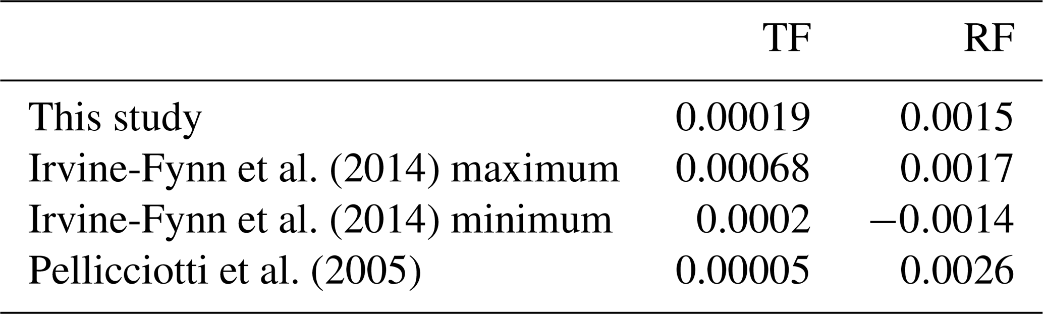
Cumulative positive T_residual and SW_net were calculated for 12 h periods beginning on 14 July at 12:00 LT. Data from 14 to 20 July were used as a training period to determine the model coefficients (η, β, TF, and RF) using multiple linear regression. The fitted model coefficients are shown in Table 1. Model coefficients compare well to those reported by Irvine-Fynn et al. (2014), a study which also modelled an Arctic glacier, although they report a wide range of values for RF depending on the training period.

Irvine-Fynn et al. (2014)Irvine-Fynn et al. (2014)Pellicciotti et al. (2005)

Table 1Model coefficients obtained using linear regression modelling for 14–20 July 2016. Units for TF are meters per hour per degree Celsius (m h^−1 ∘C⁻¹), and units for RF are meters per hour per megajoule (m h⁻¹ MJ⁻¹).

Download Print Version | Download XLSX

A 1-D formulation of the model was run at the AWS site (ETI_aws) using measured SW_net and near-surface air temperature. A distributed model (ETI_dist) was developed by estimating model variables across the study area at each grid cell. Given the relatively small size of the study area, T_residual was assumed to remain constant across the area, calculated by Eqs. (10) and (11) with modelled incoming radiation and measured temperature at the AWS site. Equations (10) and (11) can be used to back-calculate temperature when T_residual and SW_net are known; this allowed modelled temperature to vary across the grid. SW_net was calculated from modelled distributed radiation and albedo, described above.

2.4 Model performance

The four models (EB_aws, ETI_aws, EB_dist, and ETI_dist) were run for the period 00:00 LT on 1 July to 24:00 LT on 21 July 2016, allowing for comparison between models over a longer time period than when melt measurements were available. Outputs from 00:00 LT on 14 July to 24:0 LT on 31 July were compared directly to melt measured with the SR50. To compare EB_dist and ETI_dist estimates, melt values were extracted from the grid cell containing the AWS. All models were assessed using the mean and standard deviation (σ) of the residuals ($\widehat{M}-M$).

Total melt estimates for 21–24 July from both distributed models were compared to the gridded melt measurements across the study area for the same period. Model error was calculated at each grid cell in the study area; negative values indicate underestimation and positive values indicate overestimation of the model as compared to the UAV-derived data ($\widehat{M}-M$). The median model error (ME) and normalised median absolute deviation (NMAD) were used to describe the model error, following Höhle and Höhle (2009). Höhle and Höhle (2009) suggest using these metrics to describe errors when the error distributions are non-normal, which is typical for the large datasets produced with SfM (Montgomery and Runger, 2007). In the case of non-normal distributions, standard descriptive statistics (based on data means and standard deviations) are disproportionately influenced by outliers, which the ME and NMAD are not (Maronna et al., 2006). The median and range of measured and modelled melt were also calculated for comparison.

In addition to model performance, the model error across the study area was used to investigate factors influencing model performance. We examined model errors in relation to surface characteristics which are known to influence the energy available for melt (Hock, 2005). The Pearson correlation coefficient is often used to assess variable relationships:

where $\stackrel{\mathrm{‾}}{x}$ and $\stackrel{\mathrm{‾}}{y}$ are the variable means, and σ_x and σ_y are the variable standard deviations. As noted above, however, in the case that the mean and standard deviation are poor descriptors of a population, an alternative measure of relationship is necessary, using robust estimators for the location and variance (Shevlyakov and Smirnov, 2011). Based on Shevlyakov and Smirnov (2011), we use the median correlation coefficient to assess the relationship between model error and potential explanatory variables:

In the case of large samples such as those we have here ($n>\mathrm{1.8}\times {\mathrm{10}}^{\mathrm{7}}$), p values are not a suitable measure for correlation significance (Maronna et al., 2006); instead we evaluate the strength of the correlation based on its value. Robust correlations were computed between model error and terrain variables (slope and aspect), albedo, and an estimate of surface water flow.

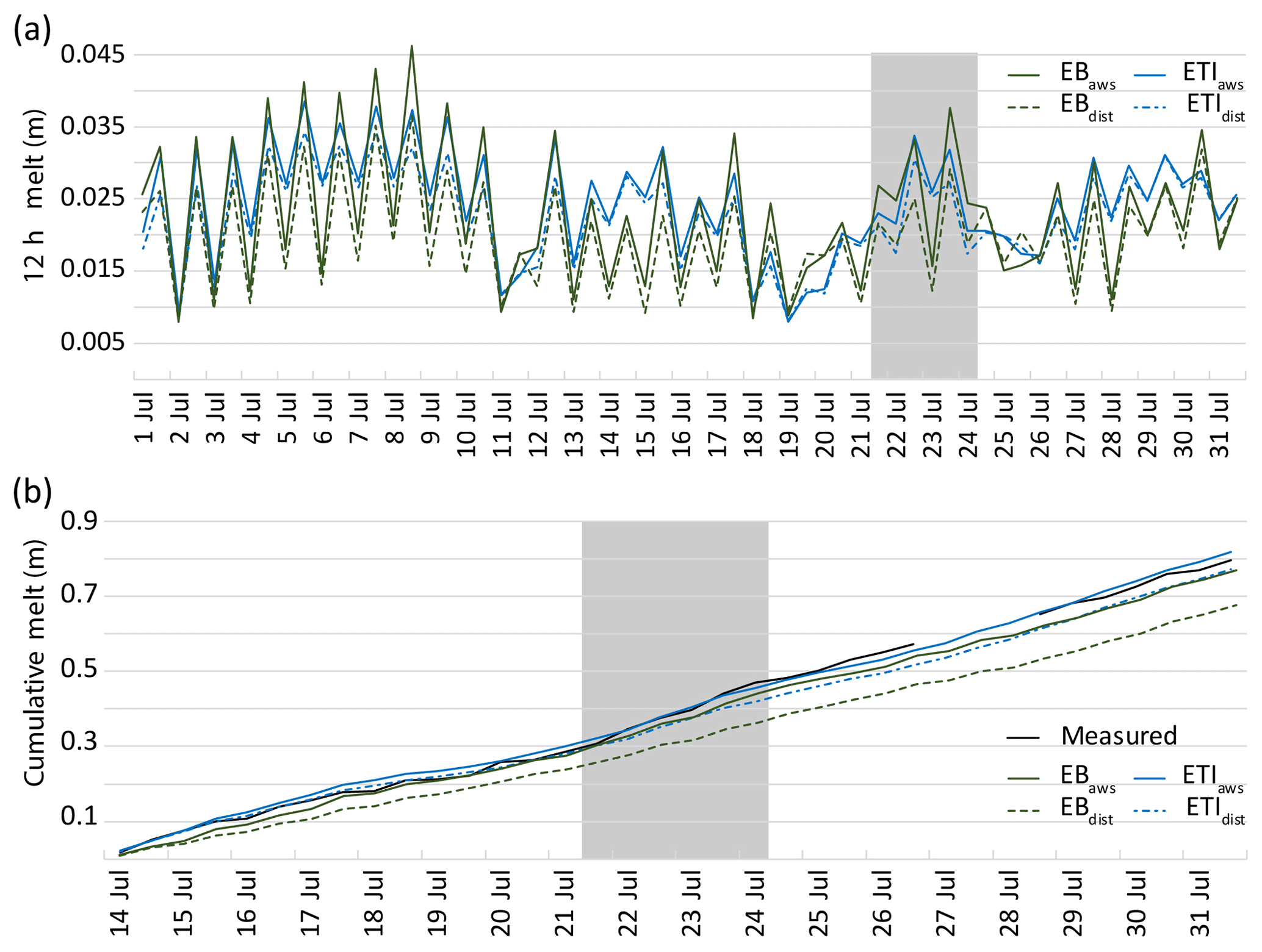
Figure 4(a) Modelled 12 h melt values at the AWS site on 1–31 July 2016. (b) Cumulative measured and modelled melt at the AWS on 14–31 July 2016. SR50 measurements were only available for the second half of July, and a gap exists in the record due to melt out of the pole holding the SR50. Melt was extrapolated during this time for better visual comparison, and extrapolation was based on average melt rates for the day prior to and following the gap. The dates of the UAV study are shown in grey.

Download

Water flow direction and potential upstream catchment were quantified using the Hydrology toolset in ArcGIS 10. Assuming that water is produced at every grid cell, flow paths were calculated from the 21 July DSM based on potential upstream accumulation. Cells with more than 1500 upstream cells were converted into a set of linear features, and the number of these features within 20 m of each grid cell was calculated (W_20 m). The 1500-cell threshold represents 15 m² of upstream drainage area and was chosen based on the assumption that 15 m² is likely to provide enough meltwater to start flow. The resulting layer provided a representation of areas with significant surface water flow, including streams and thin sheet flows.

3.1 Inter-model comparison at AWS

The four models were compared at the AWS site for 1–31 July 2016. All four models capture daily patterns of melt, with lower melt totals on average in the second half of the month, which is consistent with lower solar radiation recorded at the AWS (Figs. 4a and 2b). The distributed models both consistently estimate lower melt totals than their point model counterparts, with differences more pronounced when melt values are high. This is most likely related to the lower shortwave radiation in the distributed model, which is in total 17 % less than measured for the study period (Fig. 2b). The EB models produce lower melt estimates than the ETI models when solar radiation is low. During periods of high incoming solar radiation, EB_aws and ETI_aws produce similar melt.

The total melt estimated during the month of July was lower in the two distributed models, EB_dist=1.223 m and ETI_dist=1.394 m, compared to the point models, EB_aws=1.436 m and ETI_aws=1.508 m. The EB models estimate less melt for the month than the ETI counterparts.

3.2 Model performance at AWS site

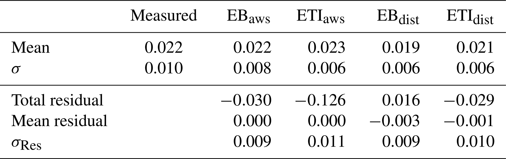
Model estimates from 14 to 31 July 2016 were compared to melt measured at the AWS site with the SR50. Total melt at the SR50 during the study period was 0.186±0.03 m, while the imagery-derived measurement for the same period was 0.274±0.048 m. After tuning z₀, the mean residual of 12 h model estimates at the AWS was 0.000 m for EB_aws and −0.003 m for EB_dist. The fitted ETI_aws also had a mean residual of 0.000 m, while that of ETI_dist was −0.001 m. Three of the four models underestimate melt at the site; ETI_aws overestimates melt by 0.016 m (Table 2; Fig. 4b). Both distributed models produce lower melt estimates than their point model counterparts. The largest underestimate was from EB_dist. The variability in modelled melt is notably lower than measured melt in all cases.

Table 2Descriptive statistics for measured melt, modelled melt, and model residuals at the AWS site from 14 to 31 July 2016. All values were calculated based on 12 h melt estimates and are reported in metres. We denote the standard deviation of all 12 h melt values with σ and the standard deviation of all residuals in 12 h model estimates with σ_Res.

Download Print Version | Download XLSX

3.3 Model performance over the study area

Across the study area, median measured melt was 0.184±0.048 m, and the NMAD was 0.026 m (Fig. 5b). Median melt across the area was lower in both EB_dist and ETI_dist, as was the variability (Fig. 5a and c). The total range of measured melt was 0.305 m, while the range of EB_dist is 0.123 and ETI_dist is 0.083.

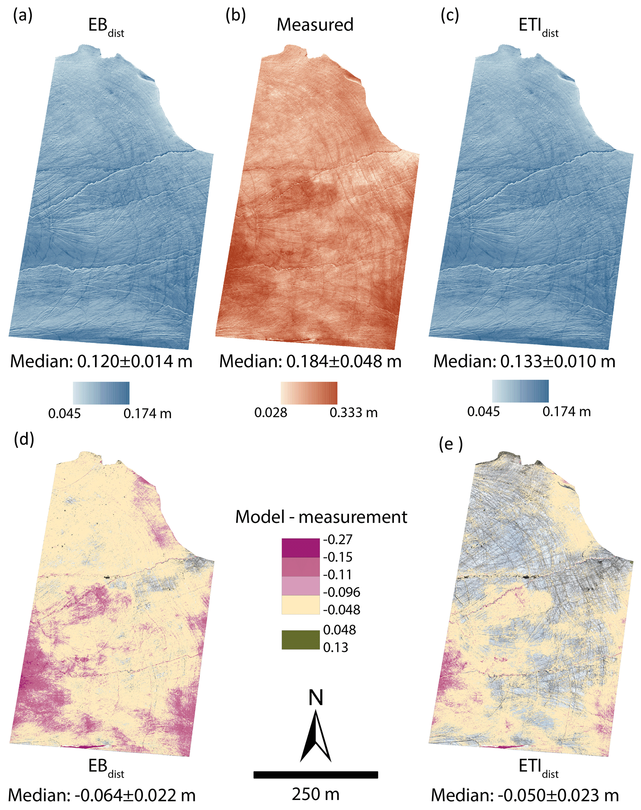
Figure 5Distribution of measured and modelled melt across the study area between 21 July (12:00 LT) and 24 July (12:00 LT). (a) Melt estimated using EB_dist applied across the study area. (b) Melt measured through differencing surfaces reconstructed from UAV imagery. (c) Melt estimated using ETI_dist applied across the study area. (d, e) Model error, calculated by the difference between modelled and measured melt. Cells with an absolute value lower than the measurement uncertainty (0.048 m) are transparent to emphasise areas where the model residuals are high.

Download

The ME and NMAD value of EB_dist is $-\mathrm{0.064}\pm \mathrm{0.022}$, while that of ETI_dist is $-\mathrm{0.050}\pm \mathrm{0.023}$. The ME of ETI_dist is of a similar magnitude to the measurement uncertainty (0.048 m), indicating general agreement with measurements. When areas of error above the measurement uncertainty are highlighted (Fig. 5d and e), ETI_dist shows clustered patterns representing 53 % of the total study area. Errors greater than twice the uncertainty (0.096 m) account for 5 % of the study area. EB_dist errors greater than 0.048 m cover 79 % of the study area, while those greater than 0.096 m cover 11 %.

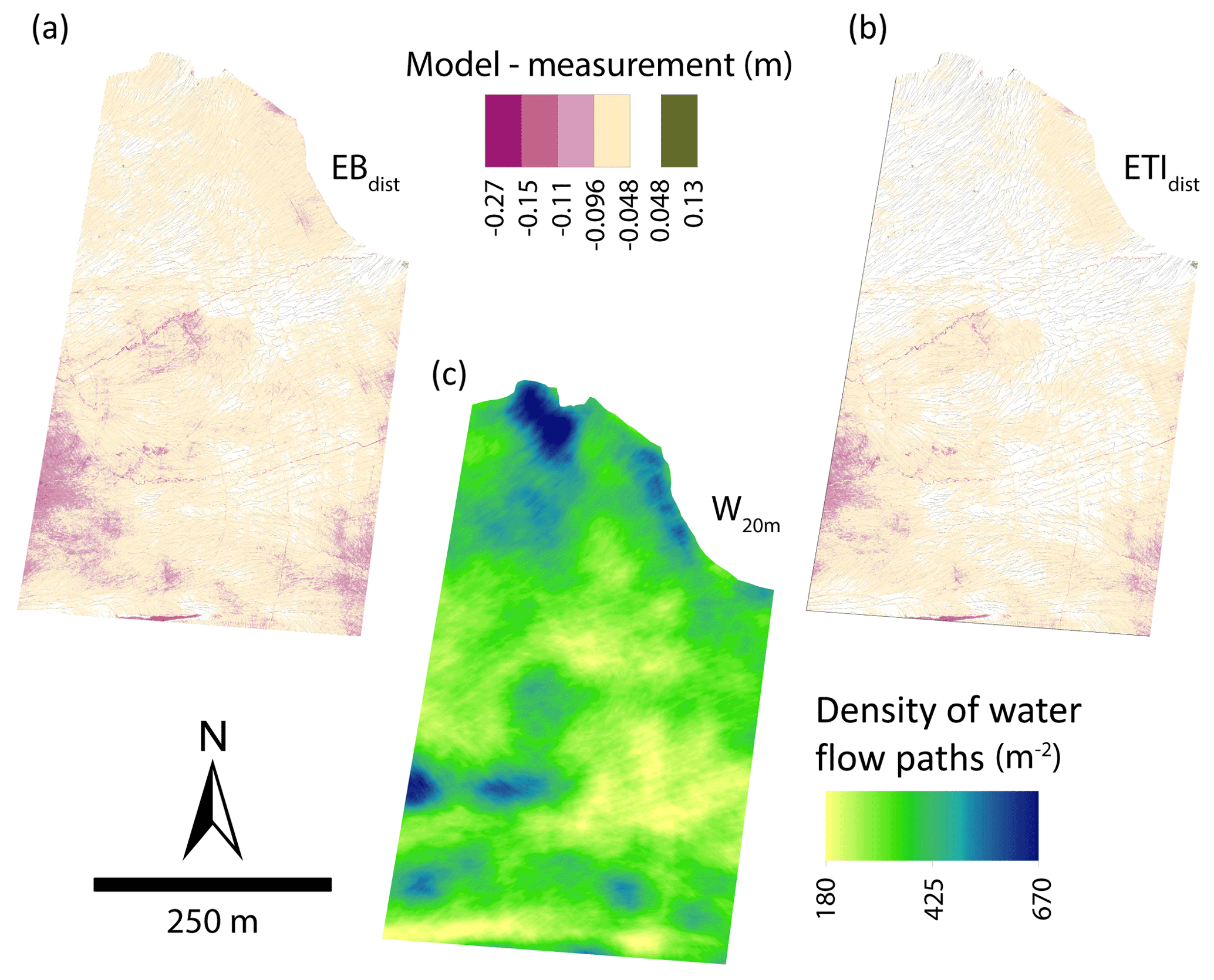
Figure 6Model error with magnitude greater than 0.048 m underlain by flow path features with potential upstream accumulation greater than 15 m² for (a) EB_dist and (b) ETI_dist. Density of flow accumulation features within a 20 m radius of each cell (c).

Download

Model uncertainty can be derived from a number of metrics, including variability in the model residuals, represented by the NMAD or standard deviation. Based on assessment at the AWS site, uncertainty in 12 h estimates from EB_dist and ETI_dist are 2σ_Res=0.018 and 0.022 m, respectively. Bash and Marshall (2014) use validation at an AWS and incorporate uncertainties related to modelling input variables to estimate an uncertainty of 15 %. In this study, we also have the benefit of examining distributed results across the study area through comparison with UAV-derived melt. The variability in the distributed models is characterised by the NMAD, taking $\mathrm{2}\cdot \mathrm{NMAD}=\mathrm{0.028}$ m for EB_dist and $\mathrm{2}\cdot \mathrm{NMAD}=\mathrm{0.044}$ m for ETI_dist; these uncertainties are 4 %–6 % of total estimated melt. The total uncertainty in the model errors can be derived using these uncertainties in combination with the uncertainty in measured surface change (0.048 m): $\sqrt{(\mathrm{2}\cdot \mathrm{NMAD}{)}^{\mathrm{2}}+{\mathrm{0.048}}^{\mathrm{2}}}$. This gives total uncertainties of EB_dist=0.056 m and ETI_dist=0.065. In either case, the errors which are strongly correlated with W_20 m are higher than the combined uncertainty of the measurement and model, particularly for ETI_dist.

3.4 Relationship to surface characteristics

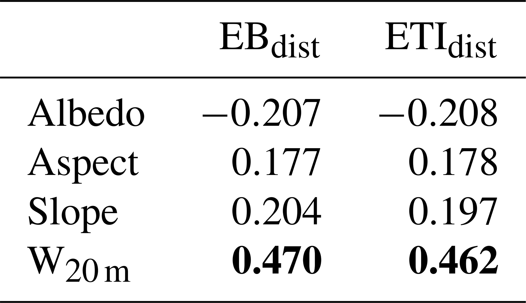
Moderate correlation was found between model error and albedo, aspect, and slope for both EB_dist and ETI_dist (Table 3). Through field observation, we were able to note a visual relationship between surface water features and high error during analysis (Fig. 6a and c). This association was confirmed through correlation with W_20 m, R_r=0.470 for EB_dist and R_r=0.462 for ETI_dist.

Table 3Robust correlation statistics (R_r) for surface characteristics and distributed models. Strong correlations are highlighted in bold.

Download Print Version | Download XLSX

Although most of the errors are negative, positive errors (i.e. overestimation) were also found. These are primarily associated with boulders and other large stationary objects on the glacier surface.