the Creative Commons Attribution 4.0 License.
the Creative Commons Attribution 4.0 License.
 | 14 Feb 2020
Glacial-cycle simulations of the Antarctic Ice Sheet with the Parallel Ice Sheet Model (PISM) – Part 1: Boundary conditions and climatic forcing
Torsten Albrecht
Ricarda Winkelmann
Anders Levermann
Simulations of the glacial–interglacial history of the Antarctic Ice Sheet provide insights into dynamic threshold behavior and estimates of the ice sheet's contributions to global sea-level changes for the past, present and future. However, boundary conditions are weakly constrained, in particular at the interface of the ice sheet and the bedrock. Also climatic forcing covering the last glacial cycles is uncertain, as it is based on sparse proxy data.
We use the Parallel Ice Sheet Model (PISM) to investigate the dynamic effects of different choices of input data, e.g., for modern basal heat flux or reconstructions of past changes of sea level and surface temperature. As computational resources are limited, glacial-cycle simulations are performed using a comparably coarse model grid of 16 km and various parameterizations, e.g., for basal sliding, iceberg calving, or for past variations in precipitation and ocean temperatures. In this study we evaluate the model's transient sensitivity to corresponding parameter choices and to different boundary conditions over the last two glacial cycles and provide estimates of involved uncertainties. We also discuss isolated and combined effects of climate and sea-level forcing. Hence, this study serves as a “cookbook” for the growing community of PISM users and paleo-ice sheet modelers in general.
For each of the different model uncertainties with regard to climatic forcing, ice and Earth dynamics, and basal processes, we select one representative model parameter that captures relevant uncertainties and motivates corresponding parameter ranges that bound the observed ice volume at present. The four selected parameters are systematically varied in a parameter ensemble analysis, which is described in a companion paper.
- Article
(13741 KB) - Companion paper
- BibTeX
- EndNote


Process-based models provide the tools to reconstruct the history of the Antarctic Ice Sheet, leading to a better understanding of involved processes and thresholds regarding the ice sheet's evolution in the past as well as in the future (Pattyn, 2018). However, ice sheet modeling involves various sorts of uncertainties. The stress balance and thickness evolution of the ice sheet is approximated and discretized, which implies different sorts of internal ice-model errors that should vanish for finer model grids (Gladstone et al., 2012; Pattyn et al., 2013). Parameterizations of physical processes at the interfaces of the ice with bedrock, ocean or atmosphere, such as basal friction, isostatic rebound, sub-shelf melting or accumulation of snow at the ice surface, involve uncertain model parameters (e.g., Gladstone et al., 2017). Certain feedback mechanisms associated with self-sustained calving may be relevant to much-warmer-than-present climates but not for the last glacial cycles (Edwards et al., 2019). Coupled climate–ice sheet system models can be computationally expensive when running hundreds of full glacial-cycle simulations, depending on their complexity (e.g., Bahadory and Tarasov, 2018, using a model of intermediate complexity with about 1 kyr per day on one core). The climatic history can be instead approximated with the averaged modern climate scaled by temperature anomaly time series. Those anomalies can be based on single ice core reconstructions, which can involve significant methodological uncertainties though (Cuffey et al., 2016; Fudge et al., 2016). Uncertainties are also large for available indirect observations of boundary conditions, e.g., for the bed topography (Sun et al., 2014; Gasson et al., 2015) or till properties underneath the ice sheet and ice shelves (Brondex et al., 2017; Falcini et al., 2018). In order to gain confidence in model reconstructions and hence in future model projections, uncertain model parameters need to be constrained with observational data (Briggs et al., 2014) using a parameter ensemble analysis (Pollard et al., 2016), as demonstrated in a systematic way in a companion paper (Albrecht et al., 2020). This study motivates choices of boundary conditions and climatic parameterizations for application in large-scale paleo-ice sheet simulations and provides an assessment of the associated sensitivity of the model's response. Therefore, we run simulations of the entire Antarctic Ice Sheet with the Parallel Ice Sheet Model (Winkelmann et al., 2011; The PISM authors, 2020b) and describe a spin-up procedure for uncertain state variables, such as the three-dimensional enthalpy field or the till friction angle at the base. The hybrid of two shallow approximations of the stress balance and the comparably coarse resolution of 16 km enable computationally efficient simulations of ice sheet dynamics over the last two glacial cycles, each lasting for about 100 000 years (100 kyr; Lisiecki, 2010).
Section 1.1 describes the ice sheet model, and Sect. 2 assesses the sensitivity for parameter variations in the ice sheet model dynamically coupled to an Earth model. Sections 3 and 4 describe the used boundary conditions and climatic forcing, respectively, and discuss how they contribute to the sea-level-relevant ice volume history. Although not the primary focus of this study, the analysis is complemented by perturbation experiments concerning the onset of the last deglaciation in Appendix A. In the Conclusions we identify a subset of four relevant parameters, one for each of the uncertainty classes, as used in the ensemble analysis in a companion paper (Albrecht et al., 2020).
1.1 PISM
The Parallel Ice Sheet Model (PISM; http://www.pism-docs.org, last access: 27 January 2020; see also note on “Code and data availability”) is an open-source three-dimensional ice sheet model (Winkelmann et al., 2011; The PISM authors, 2020b) that is used in a growing scientific community for sea-level projections (e.g. Winkelmann et al., 2015; Golledge et al., 2015, 2019) and regional studies (e.g. Mengel and Levermann, 2014; Feldmann and Levermann, 2015; Mengel et al., 2016). It uses a hybrid combination of two stress balance approximations for the deformation of the ice, the shallow ice – shallow shelf approximation (SIA-SSA), which guarantees a smooth transition from vertical-shear-dominated flow in the interior via sliding-dominated ice-stream flow to fast plug flow in the floating ice shelves (Bueler and Brown, 2009) while neglecting higher-order modes of the flow. Driving stress at the grounding line is discretized using one-sided differences (Feldmann et al., 2014). Using a sub-grid interpolation scheme (Gladstone et al., 2010) the grounding-line location simply results from the flotation condition, without additional flux conditions imposed. Basal friction is interpolated accordingly. Thus, grounding-line migration is reasonably well represented in PISM (compared to full Stokes), even for coarse resolutions (Pattyn et al., 2013; Feldmann et al., 2014). Ice deformation () in response to deviatoric stresses τ (and effective stress τe=τe(τ)) can be described according to the Glen–Paterson–Budd–Lliboutry–Duval flow law, with enhancement factor E and flow-law exponent n,
Ice softness A depends on both the liquid water fraction ω and temperature T (Aschwanden et al., 2012). PISM simulates the three-dimensional polythermal enthalpy conservation for a given surface temperature and basal heat flux to account for melting and refreezing processes in temperate ice (Aschwanden and Blatter, 2009; Aschwanden et al., 2012). The energy conservation scheme also accounts for the production of subglacial (and transportable) water (Bueler and van Pelt, 2015), which affects basal friction via the concept of a saturated and pressurized subglacial till. The strength of the till below the ice sheet is strongly controlled by water pressure (Cuffey and Paterson, 2010). A time-dependent basal substrate rheology scheme allows meltwater generated at the ice sheet bed to saturate and weaken the subglacial till layer (Tulaczyk et al., 2000; de Fleurian et al., 2018). The resulting reduced basal traction allows grounded ice to accelerate. This can, in turn, cause dynamic thinning, a reduction in driving stress and ultimately a reduced ice-stream flow later on. In PISM, the hydrology-related effective pressure,
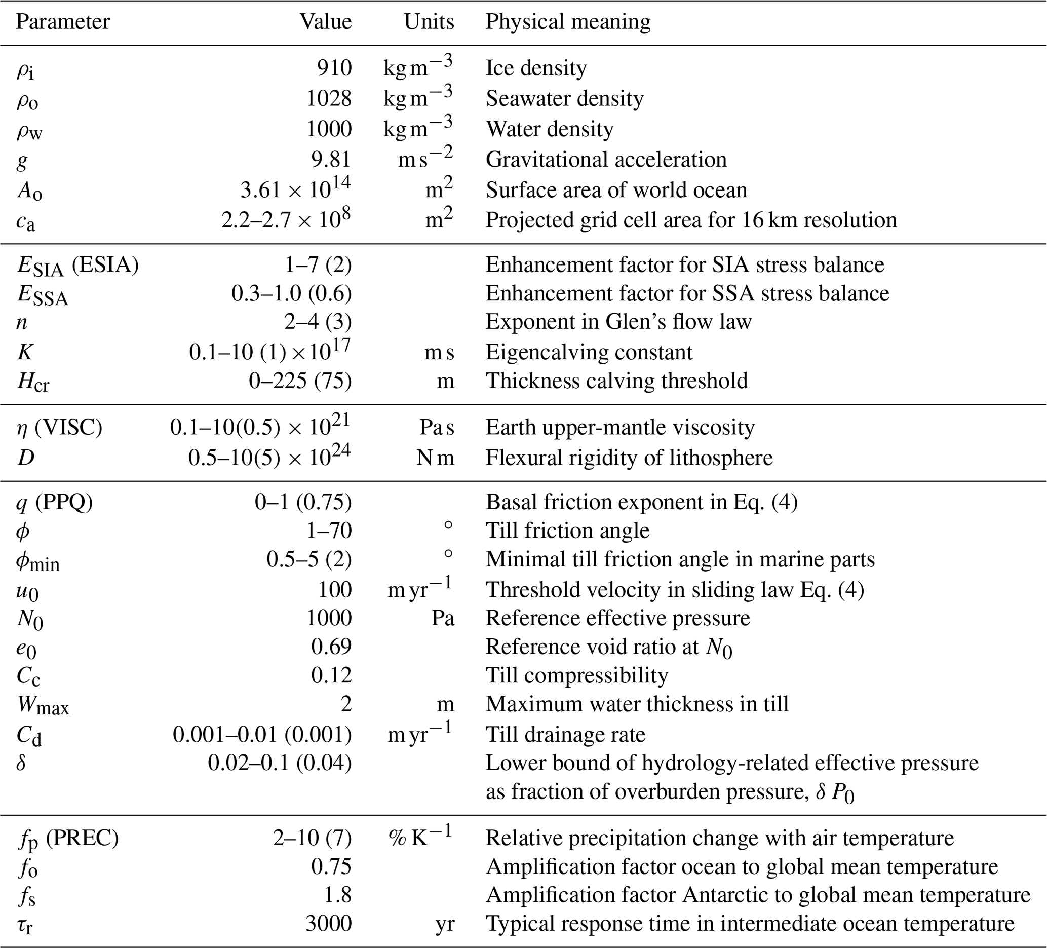
accounts for the overburden pressure P0=ρigH for a given ice thickness H and the fraction of effective water thickness in the till layer s, while all other parameters are constants (adopted from Tulaczyk et al., 2000; Bueler and van Pelt, 2015, see Table 1 for parameter meaning and values retrieved from Ice Stream B). Till water in till pore spaces is modeled in our PISM simulations as a boundary layer with an effective thickness of water content W with respect to a maximum amount of basal water and enters as fraction s in Eq. (2). For the effective pressure in Eq. (2) is hence bounded by . We use a non-conserving hydrology model that connects Wtill to the basal melt rate Mb (Tulaczyk et al., 2000), where ρw is the density of water and Cd is a fixed drainage rate,
Sliding in PISM is of the nonlinear Weertman type for sliding over rigid bedrock (Fowler, 1981; Schoof, 2010), where the basal shear stress τb (tangential sliding) is related to the SSA sliding velocity ub in the form
with being the sliding exponent and and where the Mohr–Coulomb failure criterion (Cuffey and Paterson, 2010) determines the yield stress τc (here valid for all ) as a function of small-scale till material properties (till friction angle ϕ) and of the effective pressure Ntill on the saturated till,
With a modeled distribution of yield stress, this allows for grow-and-surge instability (Feldmann and Levermann, 2017; Bakker et al., 2017).
Iceberg formation at ice shelves is parameterized based on spreading rates (Levermann et al., 2012). Ice shelf melting is calculated using the Potsdam Ice-shelf Cavity mOdel (PICO), which considers ocean properties in front of the ice shelves and simulates vertical overturning circulation in the ice shelf cavity (Reese et al., 2018).
PISM uses a modified version of the Lingle–Clark bedrock deformation model (Bueler et al., 2007), assuming an elastic lithosphere and a resistant asthenosphere with viscous flow in the half-space below the elastic plate (Whitehouse, 2018). The computationally efficient bed deformation model has been improved to account for changes in the load of the ocean layer around the grounded ice sheet due to changes in global mean sea-level height and ocean depth.
A continental-scale representation of modern bed topography is obtained from the Bedmap2 dataset (Fretwell et al., 2013) and modern uplift rates as the initial condition from Whitehouse et al. (2012). We simulate the entire Antarctic continent with 16 km grid resolution, compatible with the definition of the initMIP model intercomparison project (Nowicki et al., 2016).
PISM paleo-simulations are initiated with a spin-up procedure using a fixed ice sheet geometry, in which the three-dimensional enthalpy field can adjust to mean modern climate boundary conditions over a 200 kyr period. Full glacial dynamics are then simulated over the last two glacial cycles with temporally varying forcing, starting in the penultimate interglacial (210 kyr BP; BP – before present; defined for reference year 1950 CE) and running until the year 2000 CE. The sensitivity of the modeled ice volume above flotation to different choices of parameters and boundary conditions is evaluated as the difference to a baseline simulation (see movie in the Supplement) that is consistent with the model configuration of the best-fit ensemble simulation presented in a companion paper (Albrecht et al., 2020, see plots in Sect. 3.3 therein).
1.2 Volume above flotation
In order to compare ice volume histories, we calculate the associated contribution to global mean sea level (in units of meters of equivalent sea-level change – m SLE). Be aware that many studies just convert grounded ice volume (in units of million km3) into more handy units of sea-level equivalents (using conversion factors between 2.4 and 2.8), without subtracting the portion of the ice volume that is grounded below flotation. If this fraction of ice resting on deep submarine beds is lost, its mass converts to water required to fill the same basin (almost) without changing sea level (Jenkins and Holland, 2007; Goelzer et al., 2019). Analogous to the “volume above flotation” by the SeaRISE model intercomparison (Bindschadler et al., 2013, Eq. 1), we define here the sea-level-relevant volume as
with the flotation height
where H is the full ice thickness above a threshold of 10 m (ice-free standard definition in PISM), ca is the area distribution among grid cells (corrected for stereographic projection), zsl−b is the water depth for current sea level zsl and b is the bedrock topography. ρo = 1028 kg m−3 and ρi = 910 kg m−3 are the densities of sea water and ice, respectively (see also Table 1). The first if statement basically means “all grounded ice”, while the second one selects the “marine grounded” part of it. For consistency reasons with the used PISM version, we use ocean water density here. In fact, a density of 1000 kg m−3 should be used instead (which is a good approximation of the equation of state of the freshened ocean water). Hence, the anomaly ΔVSLE(t) is calculated from the total Antarctic ice above flotation for current sea-level forcing zsl and evolving bedrock topography b, divided by global ocean area , relative to the value for the modern observed ice sheet (Bedmap2; Fretwell et al., 2013).
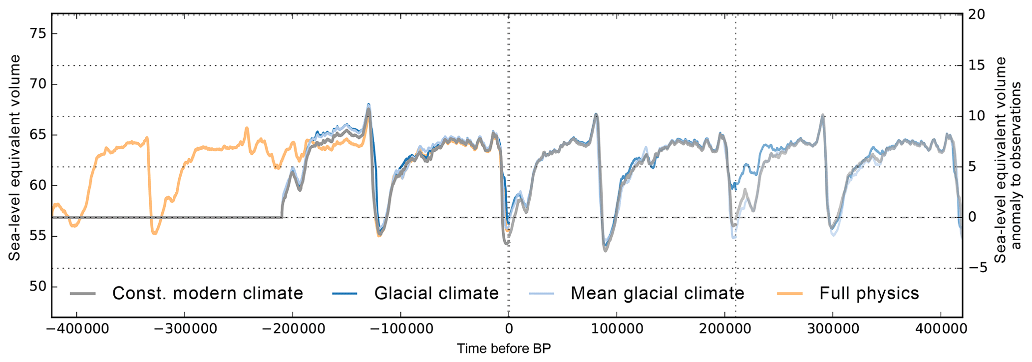
Figure 1Ice volume above flotation for simulations over the last glacial cycles with identical parameter settings but based on different spin-up procedures. The initialization method as used in the reference simulation is depicted in grey, while the orange line indicates a simulation over the last four glacial cycles. The simulations with identical initial geometry are continued into the future for repeated climate forcing of the last two glacial cycles (indicated by vertical dotted lines).
1.3 Energy spin-up procedure and intrinsic memory
In the introduction to PISM (Sect. 1.1) we briefly describe a spin-up procedure, which results in a three-dimensional enthalpy field that is in balance with the modern climate boundary conditions (see Sect. 3). We thereby assume that present-day conditions have been similar to those in the penultimate interglacial (210 kyr BP). As the three-dimensional enthalpy field carries the memory of past climate conditions, a more realistic spin-up climatic boundary condition might be achieved when the temperature reconstruction of the previous two glacial cycles (423–210 kyr BP; see Sect. 4.2) or the long-term mean over this period was used as anomaly forcing, while the ice sheet geometry remains fixed at present-day observations (Bedmap2; Fretwell et al., 2013). In the case of a simulation over the last four glacial cycles (423 kyr BP), in which the ice geometry can evolve, we can assume an even more realistic enthalpy distribution. Here we investigate the extent to which the choice of the temperature forcing in the enthalpy field spin-up can affect subsequent full-dynamics simulations over the last two glacial cycles until the present.
Three simulations are conducted with identical model settings and climate forcing but different initial energy states. The modeled ice volumes converge at the Last Glacial Maximum (LGM; 15 kyr BP) with less than 0.2 m SLE difference among the simulations, but they differ for present-day conditions by up to 2 m SLE (see blue and light blue lines in Fig. 1; at time 0 kyr BP). The reference simulations, based on the initial state that was spun-up with comparably warm constant modern climate, tend to show earlier and stronger deglaciation than the other simulations using glacial climate or mean glacial climate for the thermal spin-up. Also the full-physics simulation with glacial climate over four glacial cycles converges against the reference simulation and reveals about 1 m SLE differences to the reference ice volume evolution at present (orange line in Fig. 1).
In order to evaluate how long the memory to the initial thermal state lasts, we continue the simulations with repeated glacial climate forcing but different present-day geometries for another 2×210 kyr. Instead of converging ice volume time series, we find 1–2 m SLE divergence during interglacial states. As deglaciation reveals a nonlinear threshold behavior, it can amplify small differences in LGM ice sheet geometry. Ice thickness variations of up to 1000 m at the final interglacial state (see Fig. 2; at time 420 kyr after present) are found mainly in the large ice shelf basins of the Ross (Siple Coast), the Amery and the Ronne–Filchner Ice Shelf in the Weddell Sea, mostly determined by the migration of the grounding line. Hence, the remaining standard deviations of about 1 m SLE (for this small sample) can be interpreted as internal ice-model uncertainty and should be kept in mind when comparing and evaluating ensembles of Antarctic ice volume reconstructions. Comparably small differences in initial conditions (that can potentially be amplified) could be also related to numerical settings, such as number of used CPUs for parallel simulations.
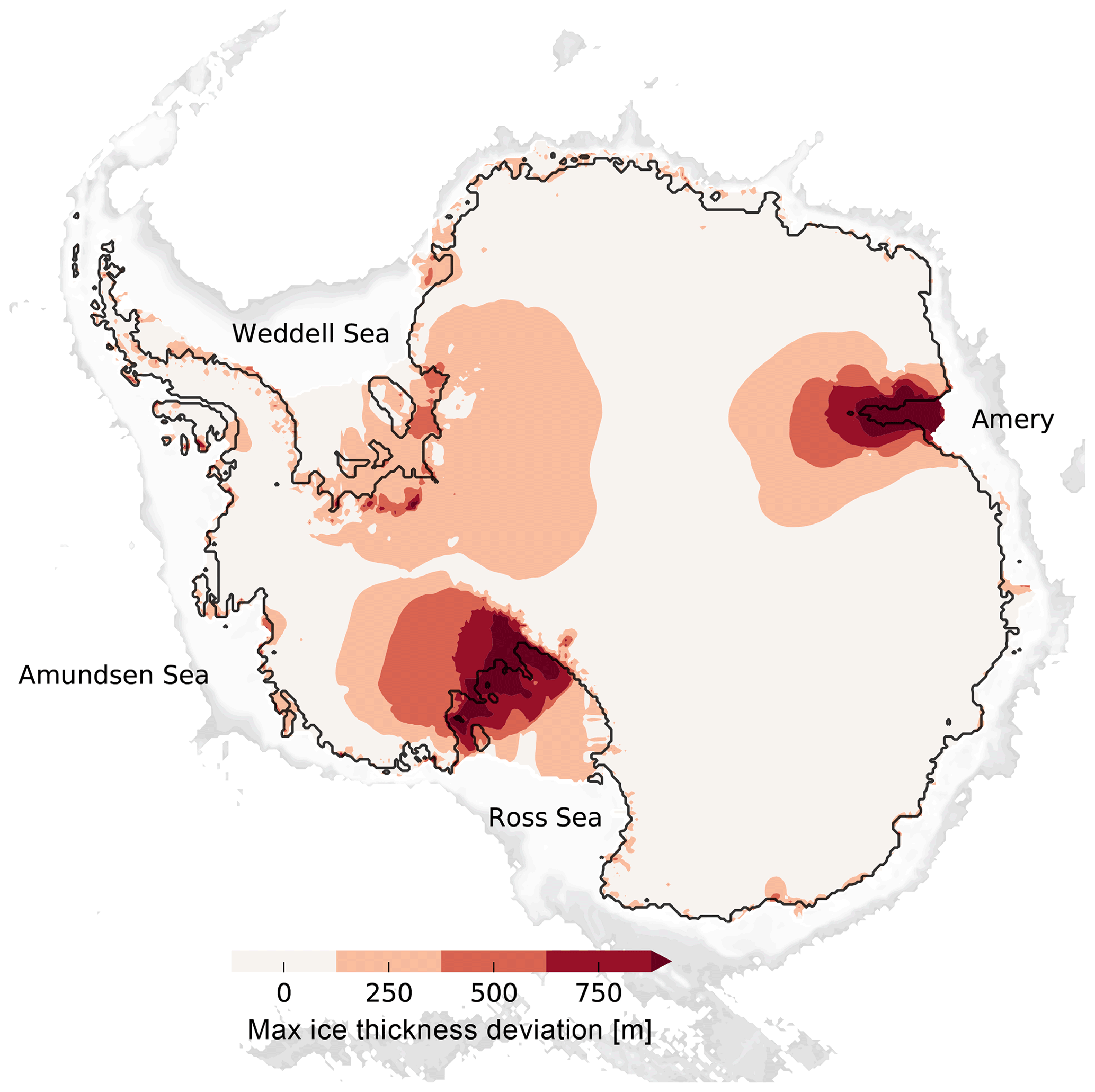
Figure 2Maximum difference in present-day ice thickness of three simulations of the Antarctic Ice Sheet after three rounds of two-glacial-cycle simulations with identical model settings but for different initial enthalpy states (cf. final state in Fig. 1). In particular the Siple Coast (Ross) and Amery trough show more than 1 km difference in ice thickness between the final states.
In the following sections we will discuss different choices of model parameterizations, boundary conditions and climatic forcings on the sea-level-relevant Antarctic Ice Sheet history over the last two glacial cycles. A summary of the corresponding sensitivities at the Last Glacial Maximum and present-day state can be found in Table 2.
Table 1Physical constants and parameter values used in this study, grouped into ice and Earth dynamics, basal sliding and subglacial hydrology, and climatic forcing. For varied parameters, the range is indicated, with the reference value in parentheses.
PISM solves a coupled system of model equations for the conservation of energy, momentum and mass. Model equations are discretized using a regular rectangular grid of 16 km resolution. Equations of stress balance are simplified using a hybrid of the shallow approximations SIA and SSA, which allows PISM to run glacial-cycle simulations. In order to close the system of equations, ice sheet models commonly use a flow law (Eq. 1), which relates ice flow to stresses. It is a result of empirical measurements and statistics for rather idealized conditions such that the flow-law-fitting exponent n comes with significant uncertainty. Enhancement factors compensate for unresolved rheological effects, e.g. anisotropy. In this section we want to understand effects of ice sheet and Earth model parameter variations on the transient glacial-cycle ice sheet response.
2.1 Ice flow enhancement factors
Enhancement factors account for unresolved effects of grain size, fabric and impurities and have often been used as tuning parameters in ice sheet modeling entering the constitutive flow law (Eq. 1) that balances strain rates and stresses within the ice sheet. A value of 1.0 means “no enhancement”, but generally enhancement factors for the SSA tend to be smaller than 1.0 and larger than 1.0 for the SIA. Anisotropic ice-flow modeling suggests ESSA values between 0.5 and 0.7 for ice shelves and between 0.6 and 1.0 for ice streams, while for SIA enhancement factors they should lie between 5.0 and 6.0 (Ma et al., 2010). Previous model ensembles that consider isotropic ice flow use values down to ESSA=0.3 (for ESIA=1.0) in Pollard and DeConto (PSU-ISM; 2012a) or up to ESIA=9.0 (for ESSA=0.8) in Maris et al. (ANICE model; 2014), both for 20 km resolution. PISM seems to favor enhancement factors closer to 1.0 (e.g. ESSA=0.5–0.6 and ESIA=1.2–1.5 in Golledge et al., 2015, for 10–20 km resolution).
Figure 3 shows the effects of ice flow enhancement factors on the simulated Antarctic Ice Sheet history. SIA enhancement generally produces thinner grounded ice. Compared to the reference simulations with ESIA=2.0 the model simulates ice sheets for ESIA=1.0 that are more than 5 m SLE thicker and ice sheets for ESIA=5.0 that are about 6 m SLE thinner, both at glacial and interglacial states (dark and light blue). The effect of ESSA variation is most predominant for ice sheet growth and for deglaciation, when ice flow across the grounding line influences its migration and stabilization (Schoof, 2007b). For ESSA=1.0 (orange) we find earlier retreat and hence 1–2 m SLE thinner modern ice sheets than for ESSA=0.6 (grey reference). For lower values of ESSA=0.3 (light orange), in contrast, deglaciation is limited and modern ice volumes are more than 5 m SLE thicker than observations. Small values for the SSA enhancement factor produce slower and thicker ice streams and ice shelves. However, as the SIA enhancement factor, ESIA, has a larger influence on the ice sheet's volume on glacial scales, we find it a more suitable ice-internal parameter candidate for the ensemble analysis in Albrecht et al. (2020).
2.2 Ice rheological flow-law exponent
Generations of ice sheet modelers used variants of Glen's flow law (Eq. 1) as the constitutive relationship between stress and internal flow with the rheological exponent n=3. According to an analysis of data in Greenland by Bons et al. (2018) the ice rheological exponent for the SIA stress balance should instead be n=4. For the same strain rates at a reference pressure of 50 kPa, we would need to adjust the ice softness factor A accordingly.
We tested the effect of the flow-law exponent n=4 (and n=2 to cover the range according to Goldsby and Kohlstedt, 2001) in comparison to the reference simulation and found only small differences in the ice volume time series during glacials and moderate differences in interglacial periods, with on average less than 0.9 m SLE difference (Fig. 4). However, the flow-law exponent for the SSA has much stronger effects on ice volume, with 2–7 m SLE less Antarctic ice volume for n=4 and significantly earlier deglaciation, while for n=2 deglaciation is effectively damped.
2.3 Model grid resolution
Resolution is a key parameter which determines the misfit between the model results based on discretized model equations and the associated analytical solutions. Analytical solutions for the coupled system of ice sheet model equations, however, can only be found for simplified configurations. For the more realistic case we can get some impression of resolution requirements if we run regression tests to show that grid refinement leads to a convergence of the model solution (Cornford et al., 2016). The horizontal resolution of the boundary data, for instance, can control key parameters of ice-stream flow, such as basal roughness (Falcini et al., 2018). Here we also test for the vertical resolution of the three-dimensional enthalpy field. In order to deal with the changing geometry of the ice, especially in the case of a non-flat moving bed, the independent variable z relative to the geoid is replaced in PISM by the vertical coordinate relative to the base of the ice. The vertical resolution is highest at the ice sheet's base and lowest at the top of the computational domain using quadratic spacing. The enthalpy formulation allows the transition from cold to temperate ice (Aschwanden et al., 2012), which can form temperate ice layers of up to a few hundred meters.
We find that for our reference parameters and 16 km resolution a similar ice volume history can be reconstructed as for 8 km resolution (see Fig. 5), while computation costs are higher by about a factor of 10. For much coarser grids of the order of 30 km or more (Briggs et al., 2014, used 40 km) we find that relevant ice-stream dynamics cannot be resolved anymore in an adequate way (Aschwanden et al., 2016). In Fig. 5 we find how resolution can effect glacial–interglacial ice volume history, resulting in very different modern ice sheet configurations (see blue lines in Fig. 5). In fact, also for coarse resolutions we may find solutions that are closer to the reference simulation, e.g. by choosing different enhancement factors.
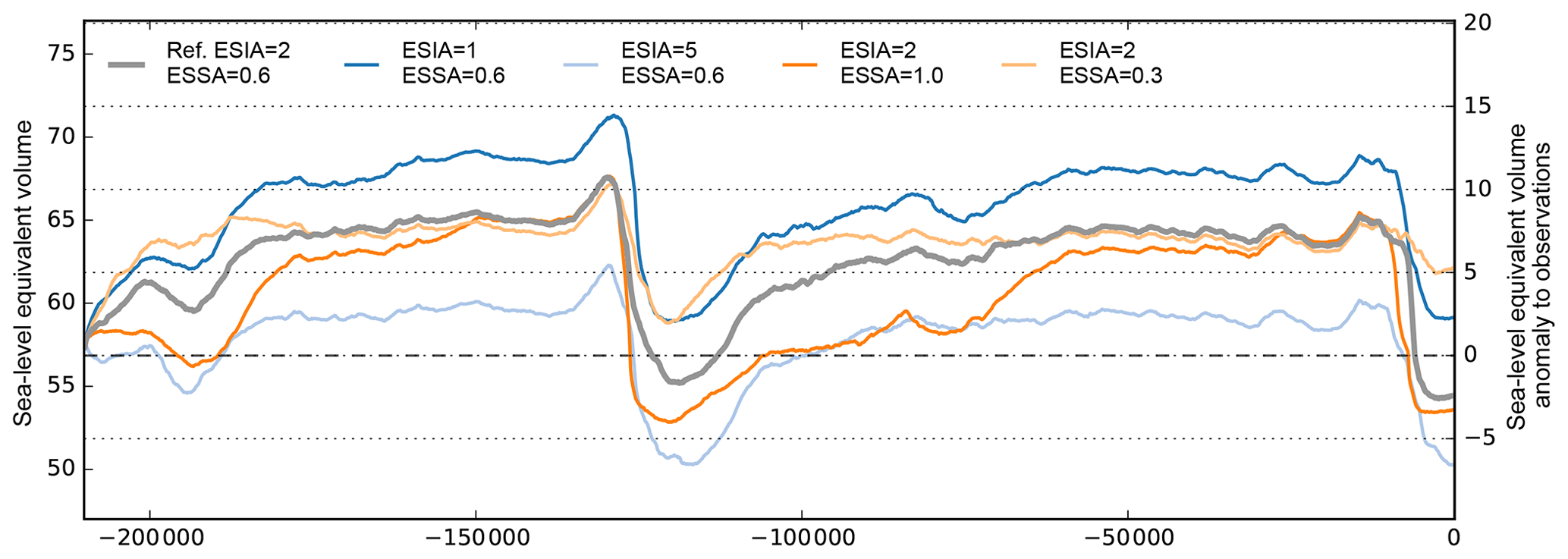
Figure 3Ice volume above flotation for simulations over the last two glacial cycles, with varied enhancement factors for SIA and SSA stress balance. Lower ESIA values lead to thicker grounded ice sheets, while larger ESSA values cause faster deglaciation and slightly thinner modern ice sheets.
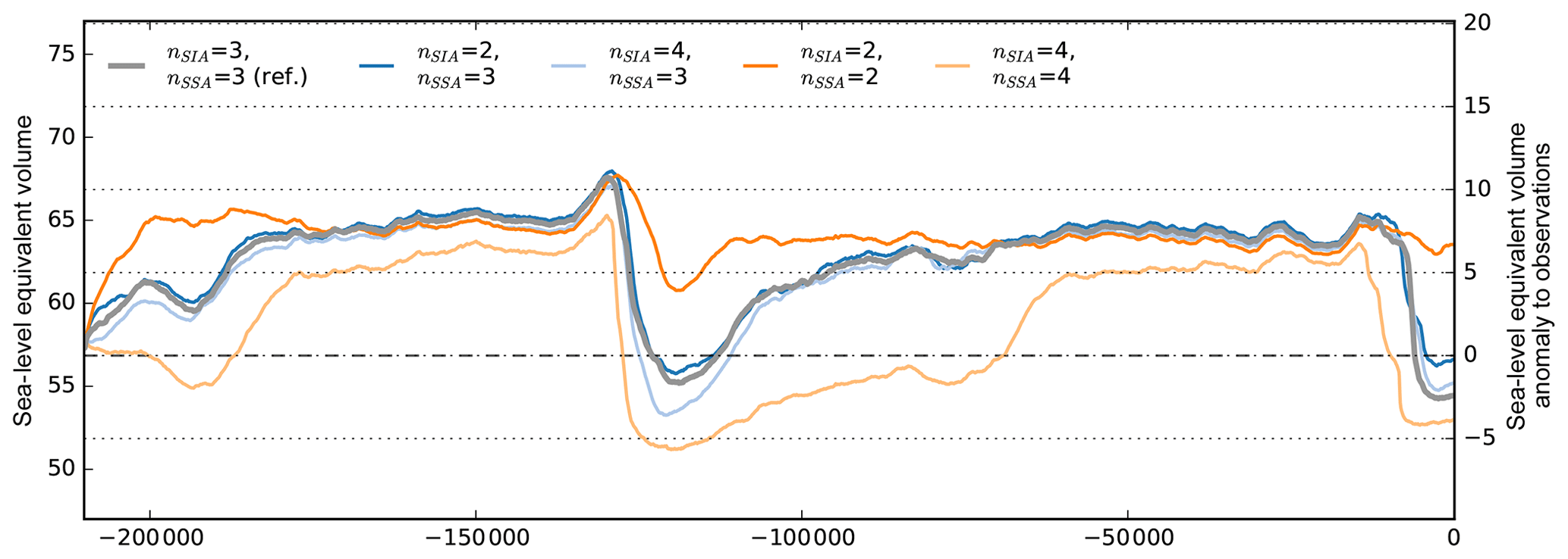
Figure 4Simulations with different flow-law exponents in the SIA and SSA stress balance, varying from 2 to 4. For variation in the SIA flow-law exponent we find only small impact on ice volume (blue, grey and light blue), while for the SSA it strongly affects ice sheet growth and deglaciation (orange and light orange).
For the vertical grid, we define, in the reference simulation, the narrowest grid spacing at the base with around 20 m. Coarser vertical resolution (doubled spacing) does not change the simulation result much (orange line in Fig. 5). For finer resolution, in contrast, shear heating and the formation of temperate ice is expected to be better resolved, and the simulation results should converge. However, the simulated ice volume seems to increase by 3–5 m SLE for doubling vertical resolution (see light orange line in Fig. 5), as less temperate ice is formed in the lowest layers of the ice sheet. Benchmark experiments with respect to an analytical enthalpy solution (Kleiner et al., 2015) suggest adequate convergence for vertical resolution finer than 1 m at the base (see violet line in Fig. 5), although this comes with much higher computational costs and memory requirements. For the used set of model parameters, such a high vertical resolution yields a present-day state close to LGM, which is 14 m SLE thicker than observed. This finding emphasizes the fact that resolution is a relevant model parameter that should be taken into account in model tuning.
2.4 Iceberg calving
Currently, calving constitutes almost half of the observed mass loss from the Antarctic Ice Sheet (Depoorter et al., 2013). PISM provides different schemes for iceberg calving. For floating ice shelves we use the strain-rate-based eigencalving parameterization, which accounts for the average tabular iceberg calving flux, depending on ice shelf flow and confinement geometry (Levermann et al., 2012; Albrecht and Levermann, 2014). The minor eigenvalue of the horizontal strain rate basically determines where calving can occur, e.g. in the expansive flow regions beyond a critical arch between outer pinning points of ice rises or mountain ridges (Doake et al., 1998; Fürst et al., 2016). The average eigencalving rate is the product of the minor and major eigenvalue of the horizontal strain rate scaled with a constant K.
In our simulations we use a reference parameter value of m s. For a much larger value of 1×10¹⁸ m s the calving front tends to retreat but is limited by the location of the compressive arch. As smaller ice shelves exert less buttressing on the ice flow, we hence find slower ice sheet growth for glacial climate conditions (see Fig. 6) but negligible effects on deglaciation or interglacial ice volume. For a smaller value of 1×10¹⁶ m s, in contrast, estimated calving rates tend to be smaller than the terminal ice shelf flow, and thus the calving front expands up to the edge of the continental shelf. The additional buttressing supports a slightly larger present-day ice volume, while in turn the more extended LGM ice shelves are more exposed to increasing sea level and ocean temperatures, leading to slightly earlier deglaciation (as already discussed in Kingslake et al., 2018).
In our simulations we define a maximum extent for ice shelves where the present ocean floor drops below 2 km depth, assuming that ice shelves can only exist on the shallow continental shelf (“deep-ocean-calv”). Additionally we avoid very thin ice shelves below 75 m, as enthalpy field evolution and hence the ice flow cannot adequately be represented for only a few vertical grid layers. Hence, ice at the calving front thinner than 75 m is removed. Both calving conditions are applied mainly for numerical reasons (adaptive time stepping) to avoid thin ice tongues, but they have negligible influence on the simulated ice volume history.
For higher lower bounds of terminal ice thickness of 150 m or even 225 m, as often used in other model studies, we find slower ice sheet growth but a negligible effect on deglaciation and interglacial ice volume (see Fig. 6). As eigencalving supports ice shelves within confinements we find that the effects of ice shelf extent beyond its compressive arch are of relatively low relevance to the glacial–interglacial ice sheet history. This is in contrast to previous model ensembles, which diagnosed high sensitivity of simulation results to varied calving parameters using different calving parameterizations (Briggs et al., 2013; Pollard et al., 2016).
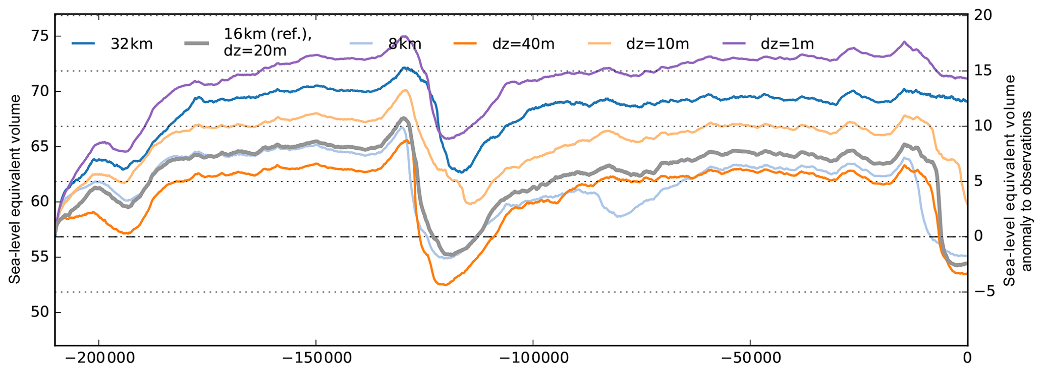
Figure 5Ice volume above flotation for simulations with horizontal reference resolution of 16 km (grey), fine grid resolution of 8 km (light blue) and relatively coarse resolution of 32 km (blue), resulting in different Antarctic Ice Sheet histories. Refined vertical resolution of 10 m (light orange) and 1 m (violet) at the base yields larger ice volumes than the reference simulation with 20 m resolution (grey) or for coarse resolution of 40 m (orange).
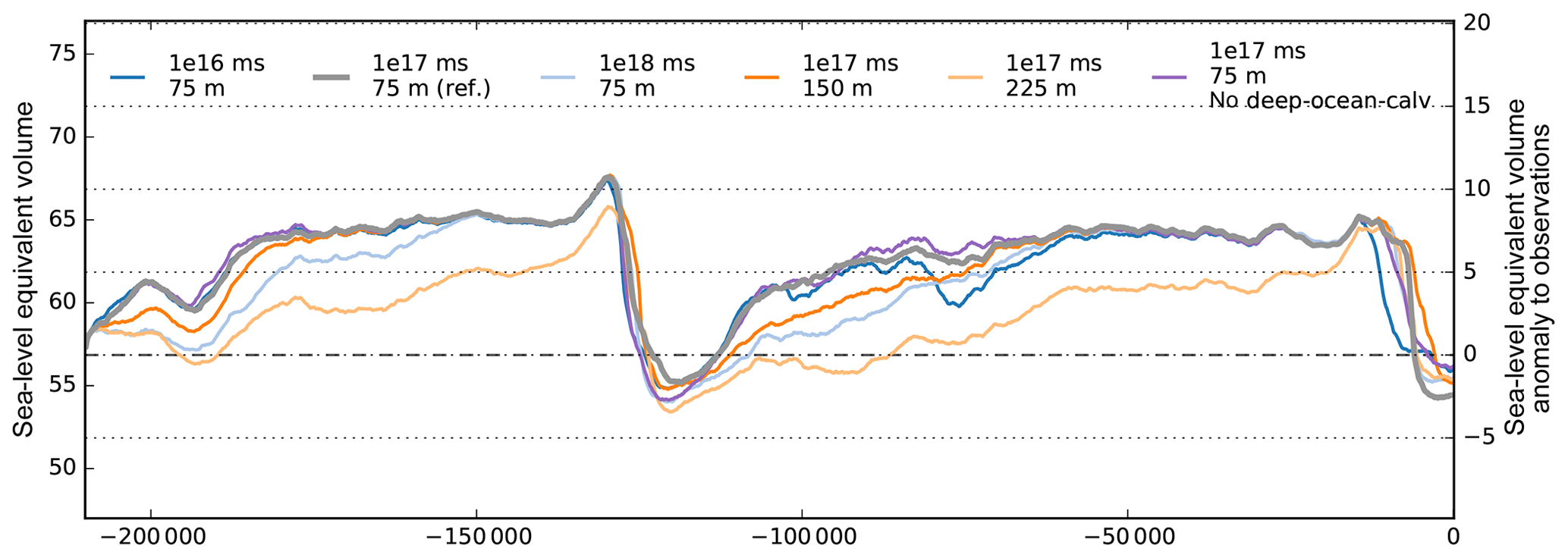
Figure 6Ice volume histories over two glacial cycles for different parameter values of eigencalving constant (blue and light blue) and calving thickness (orange and light orange) compared to the reference simulation (grey). Defining a maximum extent of the ice along the edge of the continental shelf (“deep-ocean-calv”) has only negligible effect on the sea-level-relevant ice volume (violet).
2.5 Mantle viscosity and flexural rigidity
The topography of the bed has a decisive role in the stability of the marine ice, and it can change significantly on paleo-timescales. PISM incorporates an Earth model that reflects the deformation of an elastic plate overlying a viscous half-space, based on Lingle and Clark (1985). A key advantage of this approach over traditional elastic-lithosphere–relaxing-asthenosphere (ELRA) models is that the response time of the bed topography is not considered a constant but depends on the wavelength of the load perturbation for a given asthenosphere viscosity (Bueler et al., 2007). Calculations are carried out using the computationally efficient fast Fourier transform to solve the biharmonic differential equation for vertical bed displacement in response to (ice) load changes σzz (Bueler et al., 2007, Eq. 1). The Earth model can be initialized with a present-day uplift map (Whitehouse et al., 2012) and reproduces plausible uplift pattern and magnitudes for a given load history (Kingslake et al., 2018). However, it is still a simplification of the approach used within many glacial isostatic adjustment (GIA) models (Whitehouse, 2018), which are defined to account for the response of the solid Earth and the global gravity field to changes in the ice and water distribution on the Earth's surface (Whitehouse et al., 2019). With our modification of PISM's Earth model approach we can also account for vertical bed displacement in response to spatially varying water-load changes. However, the model is not able to account for self-consistent gravitational effects associated with local sea-level variations or the rotational state of the Earth (Gomez et al., 2013; Pollard et al., 2017).
We investigate two relevant parameters of the Earth model with regard to both the viscous and the elastic part.
Mantle viscosity affects the model behavior because it defines the rate and pattern of the deformation of the ice sheet's bed and the sea floor. GIA modeling indicates a range of viscosities of 1020–1021 Pa s for the upper mantle, while the lower mantle is less constrained, with 1021–1023 Pa s (Whitehouse, 2018). Our PISM simulations distinguish neither between the upper and lower mantle nor between the East or West Antarctic Ice Sheet (EAIS and WAIS, respectively). We choose a reference value of 5×10²⁰ Pa s, although for the relatively weak mantle beneath the WAIS even lower values are likely (Gomez et al., 2015), and for some regions mantle viscosity values <1020 Pa s have been suggested (Hay et al., 2017; Barletta et al., 2018).
In our glacial-cycle simulations a lower mantle viscosity of 1×10²⁰ Pa s results in delayed deglaciation and thicker present-day ice sheets than for the reference value of 5×10²⁰ Pa s (cf. blue and grey in Fig. 7a). As the bed at the grounding line responds faster to unloading for lower viscosities, grounding-line retreat is hampered accordingly. In contrast, more viscous mantles of 25–100×1020 Pa s result in slower ice sheet growth but in faster deglaciation and hence lower present-day ice volumes above flotation (light blue and orange in Fig. 7a). Within the range of 1020–1021 Pa s the effect of mantle viscosity on grounding-line retreat and re-advance since last deglaciation has been discussed in a PISM study by Kingslake et al. (2018). In Appendix A2, we highlight the influence of further model decisions on grounding-line sensitivity and thus on the onset of deglacial retreat, although this is not the focus of this study.
The bed deformation model in PISM1 up to version 1.02 considered all changes in ice thickness H to be loads, including changes in ice shelf thickness, although this does not make physical sense. Here we present simulations that consider changes in the load of the grounded ice sheet and of the ocean layer within the computational domain, with load per unit area defined as
with hf being the flotation height as defined in Eq. (7). Be aware that since PISM v1.1 the bed deformation model has been fixed, and only the grounded ice sheet changes are considered to be a load.
Our simulations that additionally consider changes in ocean loads yield up to 3 m SLE higher ice volumes above flotation at glacial maximum and delayed deglaciation by a few thousand years, while interglacial ice volumes are comparable (cf. grey and light orange lines in Fig. 7a). The effect of changing ocean loads seems to be larger than the effect of accidentally added ice shelf loads (cf. violet line in Fig. 7b, which excludes both ocean and ice shelf loads as in PISM v1.1.
Flexural rigidity is associated with the thickness of the elastic lithosphere and has an influence on the horizontal extent to which bed deformation responds to changes in load. We have deactivated the elastic part of the Earth model in our reference simulation, as the numerical implementation was flawed. In order to evaluate the ice sheet volume's sensitivity to changes in the flexural rigidity parameter value, we used PISM v1.1 instead, with an additional fixed elastic part (https://github.com/pism/pism/pull/435, last access: 27 January 2020). However, PISM v1.1 considers only grounded ice changes to be loads and not changes in the ocean layer thickness, as in the reference. As most dynamic changes on glacial cycles occur in West Antarctica, previous studies based on gravity modeling suggest appropriate values lying within the range of 5×10²³ N m and 5×1024 N m (Chen et al., 2018). The PISM default value marks the upper end of this range, assuming a thickness of 88 km for the elastic plate lithosphere (Bueler et al., 2007).
Extending this range to 1×1025 N m, which is more than an order of magnitude, we find differences in ice volume above flotation of up to 4 m SLE, part of which might be due to increased temporal variability (see Fig. 7b). Compared to the reference simulation without the elastic part, we find earlier deglacial retreat but similar present-day ice volumes.
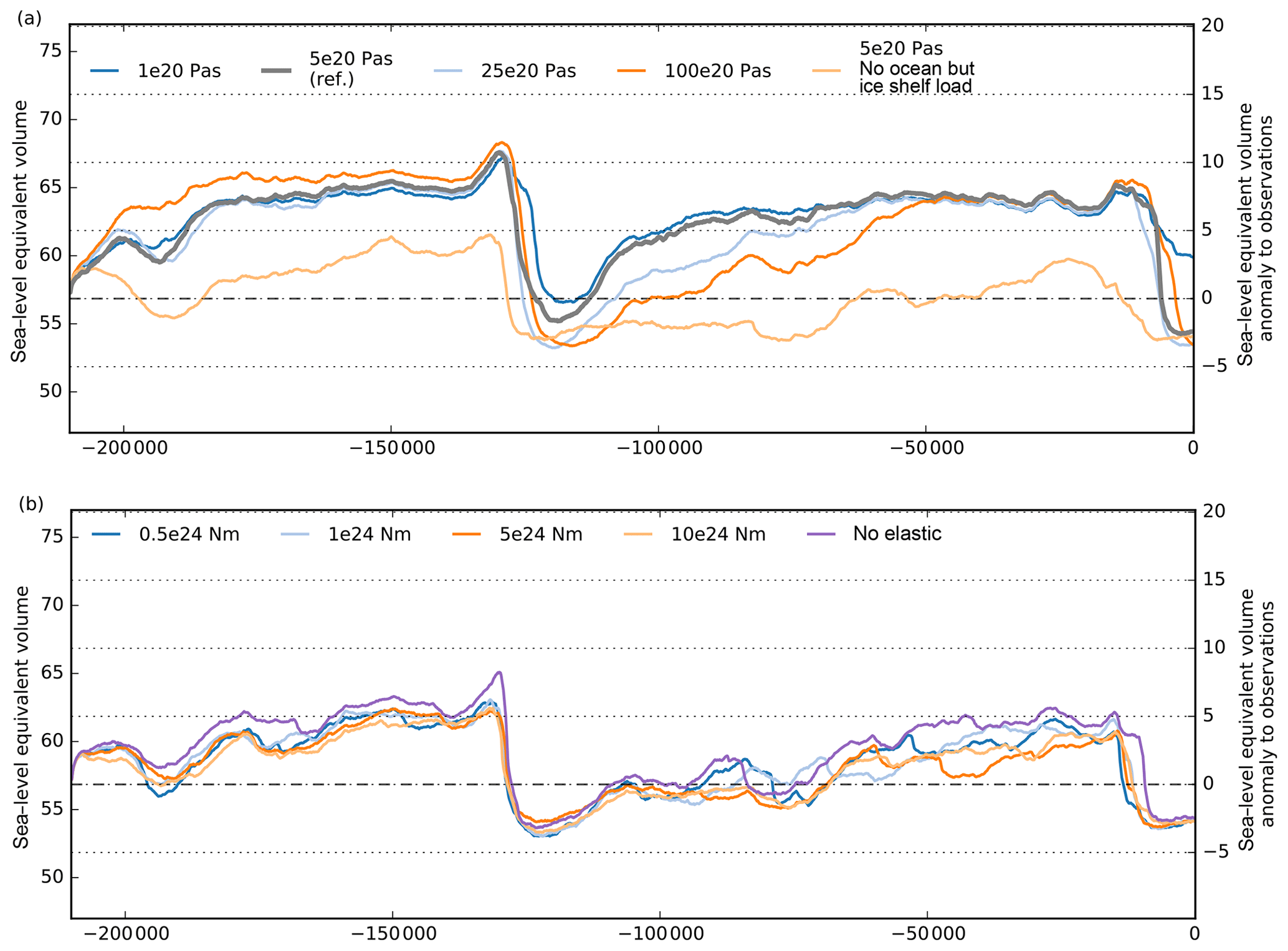
Figure 7Simulations over two last glacial cycles, with varying Earth model parameters for the viscous and the elastic part. (a) Mantle viscosities with a range over 2 orders of magnitude cause slower ice sheet growth but faster decay for increasing viscosity. (b) The tested flexural rigidity over a range of more than 1 order of magnitude yields smaller difference in simulated ice volume response but increased variability. Be aware that for (b) a different PISM v1.1 was used, with a fixed elastic model, but only accounting for changes in grounded ice loads, explaining generally lower glacial volumes than in the reference in (a).
3.1 Air temperature
Air temperature is an important surface boundary condition for the enthalpy evolution which is thermodynamically coupled to the ice flow. The annual and summer mean temperature distribution are required in the positive-degree-day (PDD) scheme to estimate surface melt and runoff rates, assuming a sinusoidal yearly temperature cycle (Huybrechts and de Wolde, 1999, Eqs. C1–3). Hitherto, surface temperatures for Antarctica have been often parameterized based on a multiple regression fit to reanalysis data, e.g., as a function of latitude “lat” and surface elevation h. This provides a temperature field that adjusts to a changing geometry with a prescribed lapse rate and is hence convenient for paleo-timescale simulations. Using ERA-Interim C20 data (Dee et al., 2011) a multiple regression fit of summer mean temperatures (January) provides a temperature distribution with a RMSE (root-mean-square error) of 2.2 K over the entire ice sheet, while for annual mean temperatures the RMSE is 4.1 K. Temperatures are considerably overestimated by up to 11 K over the large Ronne–Filchner and Ross ice shelves and in large parts of inner East Antarctica, while temperatures in dynamically relevant regions along the WAIS Divide are underestimated by up to 5 K.
Regarding the comparably shallow ice shelves with less than 100 m surface height, this surface-height-dependent parameterization estimates temperatures close to those on the sea surface, although observed climatic conditions on the large ice shelves are much colder than those on the ocean, where sea ice can be absent in summer. Typically, the Antarctic Ice Sheet and shelves inhibit a negative radiation budget that efficiently cools the surface (van Wessem et al., 2014).
As a correction we assume that the ice shelves' surface (and all other icy regions below 1000 m altitude for consistency) is as cold as at 1000 m altitude to achieve a better fit to ERA-Interim surface temperature data. Furthermore, the climate of the much larger East Antarctic Ice Sheet is more isolated than the climate in West Antarctica, which can be accounted for with a longitudinal dependence “lon” and symmetry axis through the WAIS Divide (110∘ W), as
Summer temperatures Tsml are well represented by Eq. (10), with a RMSE of 2.1 K over the entire ice sheet and a particularly good match in the large ice shelves and East Antarctica. Annual mean temperatures Taml parameterized by Eq. (9) are overestimated by less than 5 K both in the inner East Antarctic Ice Sheet and the large ice shelves of Ross and Ronne–Filchner (see Fig. 8), while temperatures in the West Antarctic Ice Sheet are underestimated by less than 1 K (RMSE 3.1 K).
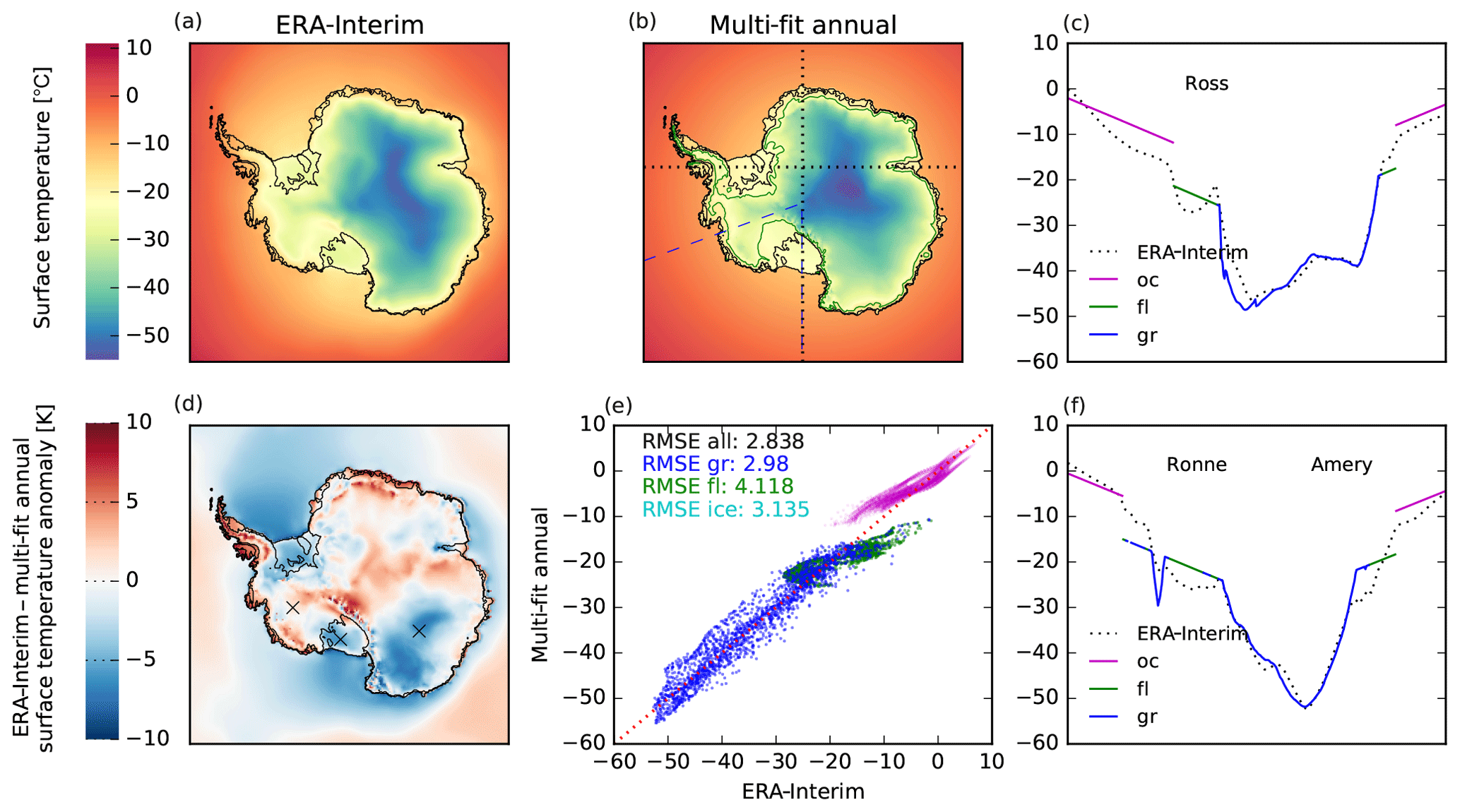
Figure 8Comparison of ERA-Interim annual mean temperatures (a) with multiple regression fit (b) according to Eq. (9), with 110∘ W longitude indicated as blue dashed line, the 1000 m surface height isoline in green and the black dotted transects through the large ice shelf regions. Inner parts of the West Antarctic Ice Sheet are less than 1 K too cold (d), while temperatures in the shallow ice shelves of Ross and Ronne–Filchner are overestimated by up to 5 K (cf. c and f). (e) Root-mean-square errors of temperatures in grounded and floating ice sheet regions are 3.0 and 4.1 K, respectively.
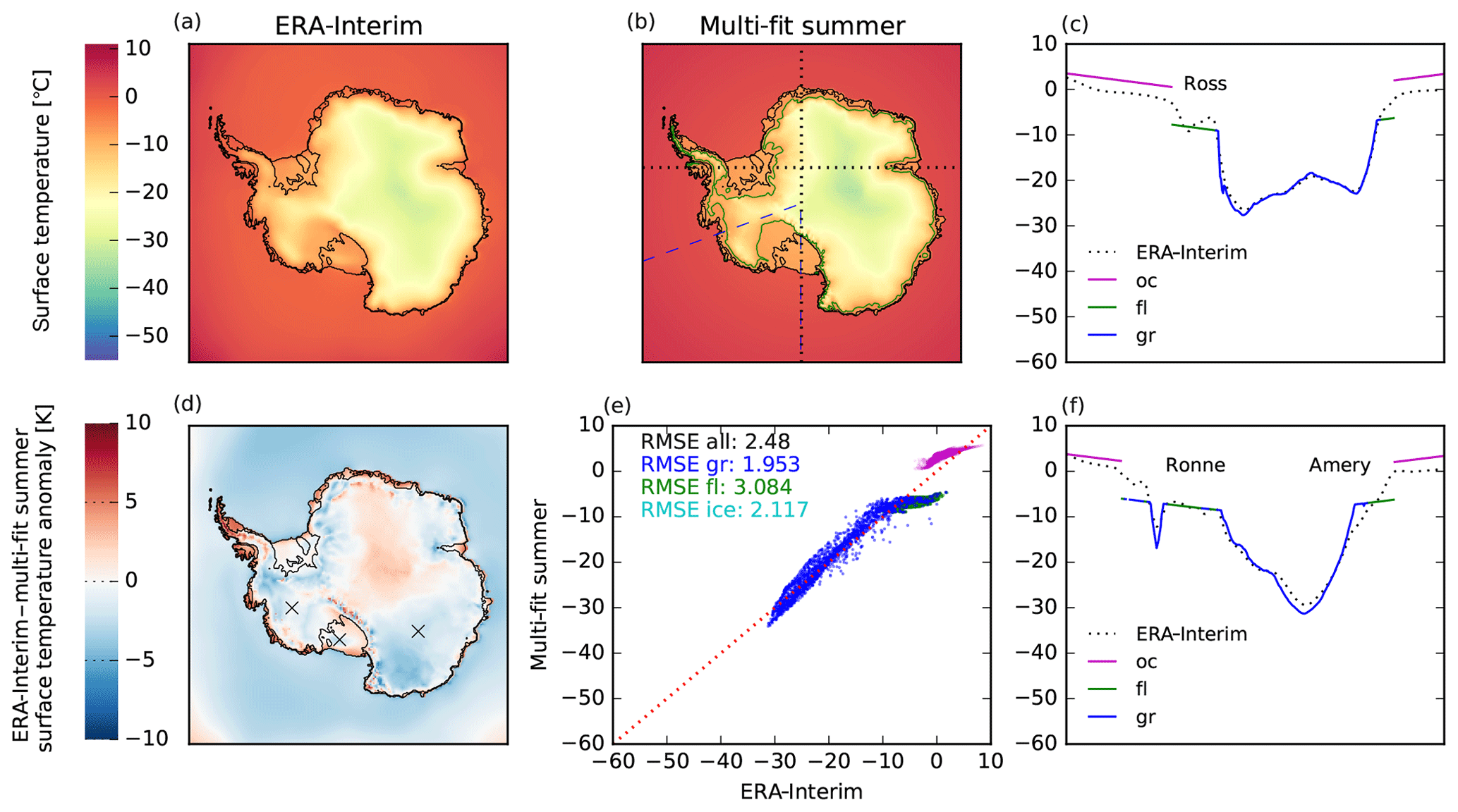
Figure 9Comparison of ERA-Interim summer (January) mean temperatures with parameterization of Eq. (10). Root-mean-square errors of temperatures in grounded and floating ice sheet regions are 2.0 and 3.1 K, respectively, with temperatures in the large ice shelves close to observations.
The annual mean and summer air temperatures enter the PDD scheme to calculate melt rates and runoff at the surface. We assume melt rates of snow and ice of 3.0 and 8.8 mm for each day and per degree above freezing, assuming a daily temperature variability represented by a normally distributed white noise signal with a 5 K standard deviation.
In order to evaluate the transient effects of the choice of the modern climate boundary conditions we run two-glacial-cycle paleo-simulations with a climatic forcing that is introduced in the following sections of the paper. Here we compare the simulated histories of the ice sheet's volume above flotation with respect to different modern surface temperatures and PDD settings. A lower temperature standard deviation in the PDD scheme of 2 K instead of 5 K has no influence on glacial volume, but it can delay deglaciation slightly (see Fig. 10). Generally, the effect of the PDD scheme for Antarctic paleo-simulations seems of minor relevance. Even if we do not parameterize the surface mass balance via the PDD scheme and directly apply the annual mean temperature pattern from the parameterization, RACMO2.3p2 (van Wessem et al., 2018) or ERA-Interim (Dee et al., 2011), to the ice surface boundary, simulated ice volumes differ at most by up to 2 m SLE.

Figure 10Ice volume above flotation for variation in PDD standard deviation and for different modern mean temperature distributions. The sensitivity is low for different PDD parameters of 5 K (reference in grey) and 2 K and when no surface model with yearly cycle is used (blue and light blue respectively), also for interglacials. For more realistic annual mean surface temperatures from RACMO2.3p2 (van Wessem et al., 2018) or ERA-Interim (Dee et al., 2011), but without PDD and yearly cycle applied, the simulated volumes show most difference for glacial ice sheet growth and at interglacials (orange and light orange, respectively).
3.2 Precipitation
The distribution of mean precipitation over the Antarctic continent is related to temperatures, but its pattern is strongly determined by the moisture transport over the ice and mountain surface such that parameterizations as for the temperature (see Sect. 3.1) are rather unrealistic. We use a more realistic precipitation field from the regional atmospheric climate model RACMO2.3p2 (van Wessem et al., 2018, as mean over CMIP5 reference period 1986–2005), which was forced with ERA-Interim reanalysis data for the recent past. RACMO2.3p2 incorporates all relevant physical processes at the ice surface simulated with a resolution of 27 km.
Analogous to the temperature parameterization, we apply a lapse correction to the RACMO precipitation field for changing surface elevation Δh to account for the elevation desertification effect (DeConto and Pollard, 2016), which we define as
with fp=7 % K−1 being a precipitation change factor according to the Clausius–Clapeyron relationship and with γT=7.9 K km−1 being the temperature lapse rate. This correction ensures that topographical changes have an influence on local precipitation through their effect on local surface temperature. However, as reanalysis and regional climate models tend to underestimate present-day precipitation in the interior of the East Antarctic Ice Sheet, simulated ice volume may be biased towards being lower than observed values (Van de Berg et al., 2005).
3.3 Basal heat flux
Geothermal heat flux is one of the most poorly known boundary conditions that controls ice flow (Pittard et al., 2016). It can keep basal ice relatively warm and thus less viscous than the colder ice above. PISM uses a bedrock thermal model (1-D heat equation, similar to Ritz et al., 1996), with storage in an upper-lithosphere thickness of 2 km discretized in 20 equidistant layers. Geothermal heat flux is applied as a constant boundary condition to calculate the heat flux into the ice at the ice–bedrock interface depending on the ice base temperature. In combination with enhanced supply of meltwater at the ice sheet base, it supports rapid ice flow by sliding over the bed and deformation of the subglacial sediments (see Sect. 3.4.2). Various maps with substantially different patterns derived from satellite magnetic and seismological data have been made available for the whole Antarctic continent (https://blogs.egu.eu/divisions/cr/2018/03/23/image-of-the-week-geothermal-heat-flux-in-antarctica, last access: 27 January 2020) and have been used in ice sheet model simulations for longer then a decade now (Shapiro and Ritzwoller, 2004; Fox Maule et al., 2005; Purucker, 2013; An et al., 2015). Due to their sparse data coverage and significant methodological uncertainty, some modelers decided to use a simplified two-valued heat-flux pattern that distinguishes the geology of the East and West Antarctic plates (Pollard and DeConto, 2012a). In our reference simulation, we use the latest high-resolution heat-flux map by Martos et al. (2017), which is derived from spectral analysis of the most advanced continental compilation of airborne magnetic data.
For the different Antarctic basal heat-flux datasets we compare PISM-simulated quasi-equilibria after 50 kyr with constant boundary conditions and find only few differences, with 40–45 m RMSE between the resulting ice thickness distributions (Fig. 11), except for the lowest estimate of basal heat flux by Purucker (2013), with about 100 m RMSE.
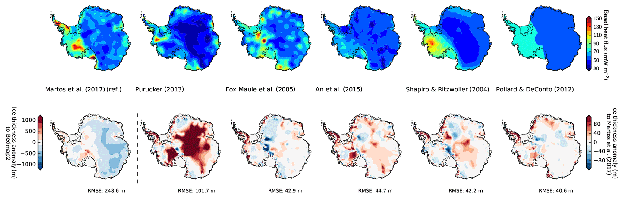
Figure 11PISM present-day equilibrium results after 50 kyr for different basal heat-flux fields (upper row) affecting the near-ground ice temperatures and hence the ice thickness, shown here for the first equilibrium result as anomaly to Bedmap2 (first panel in lower row) or relative to the first result. First three columns show the results for the magnetic reconstructions by Martos et al. (2017) (as in the reference), Purucker (2013) and Fox Maule et al. (2005). Columns 4 to 5 show the seismic reconstructions by An et al. (2015) and Shapiro and Ritzwoller (2004), and last column shows, for comparison, a two-valued field as used in Pollard and DeConto (2012a), separating East and West Antarctica. The overall effect of the choice of geothermal heat flux on present-day equilibrium ice thickness measures up to 100 m RMSE for Purucker (2013), while for the other tested set-ups it differs only in individual spots, with a RMSE of 40–45 m.
Here we compare the simulated histories of the ice sheet's volume above flotation with respect to the different basal heat-flux boundary conditions. The overall effect on ice volume history seems rather small, with a variation of about 3 m SLE for glacial climates. The lowest mean heat flux of 54 mW m−2 (Purucker, 2013) yields generally larger ice volumes and vise versa for the highest mean heat flux of 67 mW m−2 (see Fig. 12; Martos et al., 2017). The transient sea-level-relevant volume shows most variance during interglacials, when in some relevant regions of West Antarctica, such as the Siple Coast, grounding-line migration is delayed, and the local anomaly in ice thickness reaches up to 500 m. In particular for the present-day state the largest range of simulated ice volumes is found with about 8 m SLE. Compared to other uncertainties discussed in this study, e.g. with regard to friction-related parameters (see Sect. 3.4), we evaluate the choice of the basal heat-flux distribution of low relevance to the total ice volume history. However, in another PISM ensemble study that covers the last 2 million years with a focus on ice domes and deep ice cores during interglacials, geothermal heat flux becomes the most relevant uncertain boundary condition (Sutter et al., 2019). Also, the thickness of the bed thermal unit seems to be of relatively low relevance, even when compared to the extreme case of basal heat flux directly applied to the ice sheet base, without a thermal unit (see Fig. 12b).
3.4 Basal friction
Subsurface boundary conditions and their influence on basal sliding are key to understanding Antarctic ice flow, in particular subglacial topography, basal morphology (e.g., presence of sediments) and subglacial hydrology (Siegert et al., 2018). In the following section we will investigate the model's sensitivity to the pseudo-plastic exponent of the basal sliding relationship, the till friction angle under grounded ice and underneath the modern ice shelves, and parameters related to subglacial hydrology, namely the till water decay rate and the critical fraction of overburden pressure.
3.4.1 Pseudo-plastic exponent
In PISM, basal sliding is parameterized according to Eq. (4) with sliding exponent q. A value of q=0.0 represents purely plastic (Coulomb) deformation of the till where ice flows over a rigid bed with filled cavities (Schoof, 2005, 2006). Many studies use (e.g., Schoof, 2007a; Pattyn et al., 2013; Gillet-Chaulet et al., 2016) or a linear sliding relationship between basal velocity and basal shear stress for q=1.0, as most commonly adopted for inversion methods (e.g., Larour et al., 2012; Gladstone et al., 2014; Yu et al., 2017). Note that ub results from solving the non-local SSA stress balance (Bueler and Brown, 2009, Eq. 17) in which τb appears as one of the terms that balances the driving stress. The PISM default sliding velocity threshold is u0=100 m yr−1, where basal shear stress is independent of q.

Figure 12(a) Simulation results for different basal heat-flux distributions (Martos et al., 2017; Purucker, 2013; Fox Maule et al., 2005; An et al., 2015; Shapiro and Ritzwoller, 2004; Pollard and DeConto, 2012a). The range of the resulting ice volumes above flotation is rather small, with less than 3 m SLE on average. In interglacial periods the divergence in ice volume can reach more than 8 m SLE. (b) Sensitivity of transient ice volume to varied thickness of the bed thermal layer (model option “Lbz” in km, with “Mbz” the number of equidistant vertical grid subdivision of the layer; see legend). Reference thickness is 2 km (grey), which yields similar results to a 5 km thick bed thermal layer (light blue). Not taking any bed thermal unit into account leads to slightly lower ice volumes, in particular during LIG (blue).
Over the valid range of q we find a spread of reconstructed ice volumes of up to 12 m SLE (see Fig. 13) in transient simulations. Larger values lead to thinner ice sheets, in particular at interglacial states. Due to its large impact on ice volume the pseudo-plastic exponent q, or PPQ, is a key parameter in the ensemble analysis presented in a companion paper (Albrecht et al., 2020).

Figure 13Antarctic ice volume history over the last two glacial cycles for different values of the basal sliding exponent q. Between plastic (blue) and linear sliding (light orange), the ice volume above flotation can vary by 6 m SLE on average and by up to 12 m SLE in interglacial periods. Generally, smaller values of q lead to slower ice flow and hence to larger ice volumes.
3.4.2 Till properties
The till friction angle ϕ is a shear strength parameter for the till in Eq. (5), associated with the geology of the bed. It can be parameterized in PISM as a piecewise-linear function of bed elevation (Martin et al., 2011), assuming that marine basins and ice-stream fjords have a rather loose sediment material, while being denser in the rocky regions above the sea level. The till friction angle is weakly confined; the observational range in ice streams is 18–40∘ in Cuffey and Paterson (2010). For now, we assume that ϕmin=2∘ in the marine basins lower than −500 m, that ϕmax=45∘ above 500 m and that there is a linear gradient between those two levels.
We run 50 kyr equilibrium simulations, first with a spatially constant value of the till friction angle with ϕ=30∘ (Cuffey and Paterson, 2010, see Fig. 14). The simulation shows a general overestimation of ice thickness, with anomalies of more than 800 m in West Antarctica and an overall RMSE of 372 m for the constant till friction angle. When using the piecewise-linear parameterization, the anomalies are negative in large parts of the East Antarctic Ice Sheet and at the WAIS Divide, with a lower RMSE of about 296 m. This suggests that estimates of till friction angle in parts of the submarine basins are too low, while along the Siple Coast and in the Transantarctic Mountains values seem too high. Nevertheless, the dependence on fjord topography supports narrowly confined structures of simulated ice streams, similar to those observed in many Antarctic regions.
In the following we want to demonstrate how till friction angle estimates can be optimized to fit the observed grounded surface elevation (or ice thickness) from Bedmap2 (Fretwell et al., 2013). We here follow the simple inversion method by Pollard and DeConto (2012b), but we invert for the till friction angle ϕ rather than for the basal sliding coefficient τc. In PISM the effective pressure Ntill in Eq. (5) is physically determined by the subglacial hydrology model, while Pollard and DeConto (2012b) use basal temperature as a surrogate. As we run the simulation forward in time for constant boundary conditions the till friction angle is adjusted in every grounded grid cell every 500 years in incremental steps of Δϕ. These steps are proportional to the misfit to observed surface elevation (divided by 200 m) and bounded by . Since the surface elevation is underestimated in the inner parts of the East Antarctic Ice Sheet by a couple hundred meters (due to underestimated precipitation forcing), the retrieved till friction angles reach a maximum value, set here as ∘, which enhances yield stress by about an order of magnitude (see middle row in Fig. 14). In contrast, on the Siple Coast the minimum values of ∘ compensate for the overestimated ice thickness (see bottom row in Fig. 14). Thus, the RMSE of ice thickness can be significantly reduced to 141 m (or even 123 m for ∘), and the modeled ice volume is only 0.5 % below observation. The retrieved distributions of till friction angles are rather independent of initial conditions and iteration parameters (not shown here). In fact, this method may overcompensate for inconsistent model boundary conditions or processes that are not accurately represented.
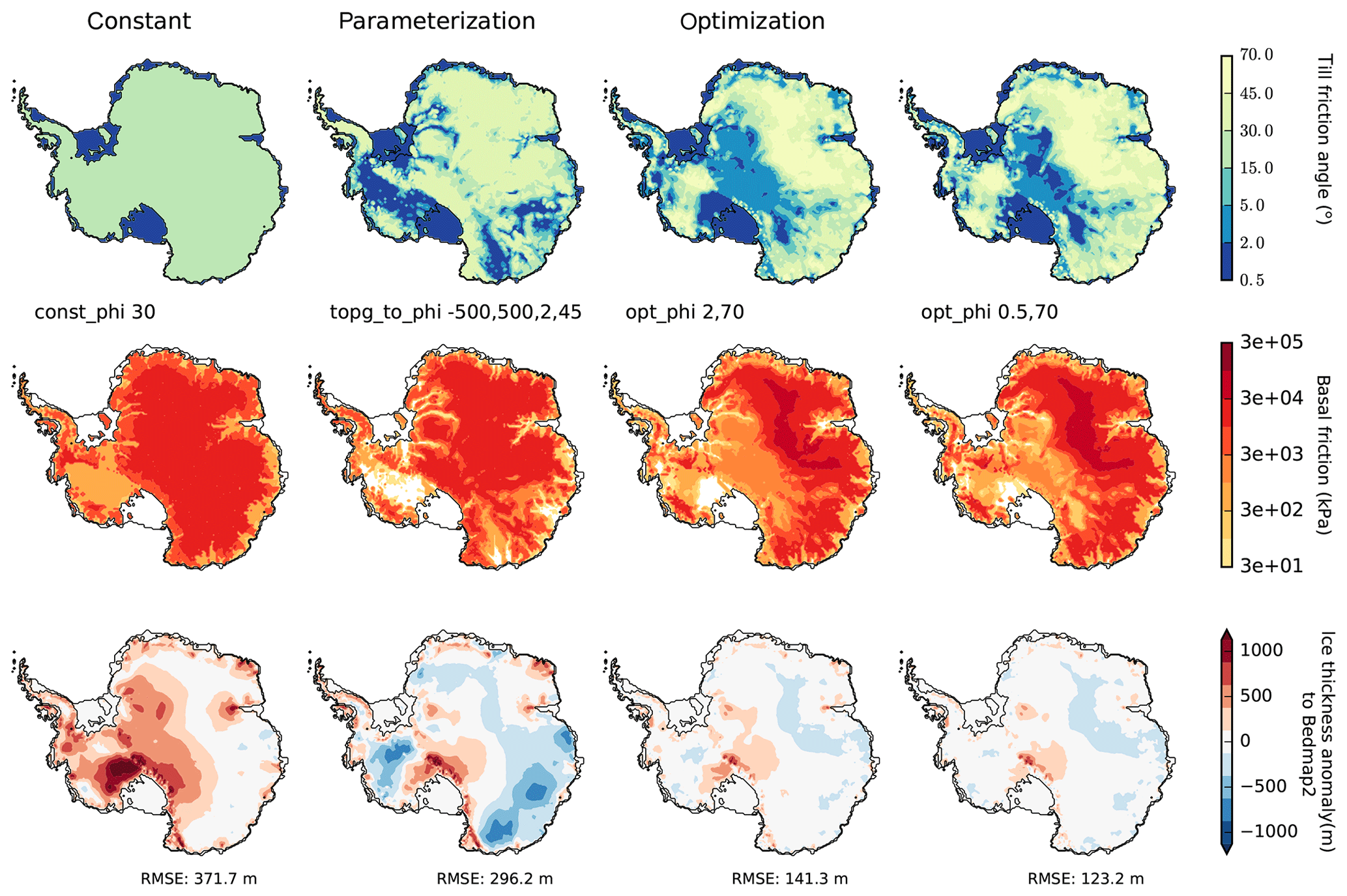
Figure 14PISM equilibrium simulations for different basal friction fields (τc in middle row) based on different till friction angle distributions (ϕ in first row). First column is with spatially uniform till friction angle of 30∘, second column shows till friction angle according to PISM parameterization as function of bed topography and last columns use a simple inversion technique with different minimal . Last row shows the resulting ice thickness anomaly to Bedmap2 observations (Fretwell et al., 2013), with improvements particularly in East Antarctica and Siple Coast region and overall RMSE reduced to 123 m (with parameters ESIA = 1 and Cd=5 mm yr−1).
For the transient response of the ice sheet's volume to the different distributions of till friction angle, we find similar glacial ice volumes for the depth-dependent parameterization and the optimization, while in contrast interglacial ice volumes differ considerably (cf. light blue and grey in Fig. 15a). For the spatially constant till friction angle of 30∘ underneath the grounded ice sheet and 2∘ on the ocean floor, we simulate glacial-cycle volume histories that are a few meters larger than for the piecewise-linear parameterization (blue). In fact, we find a much larger effect on the ice sheet volume for variations in the till friction angle on the ocean floor.
Till properties under modern ice shelves
Friction (and also bed topography) at the ocean bed underneath the modern ice shelves is poorly constrained, as the optimization algorithms only apply to modern grounded regions (e.g., Pollard and DeConto, 2012b; Morlighem et al., 2017). The friction coefficient on the continental shelf has thus been chosen as one of the ensemble parameters in Pollard et al. (2016, 2017). In PISM the till friction angle accounts for the flow properties of the substrate and enters the yield stress definition as tan (ϕ) (see Eq. 5). As sandy sediments are prevalent in the ice shelf basins, low values of ϕ are likely in these regions (Halberstadt et al., 2018). Additionally, the till friction angle in the ice shelf basins is a crucial parameter which determines the thickness of the extended ice sheet for LGM conditions and hence the potential contribution to the global sea-level change.
Modeled LGM ice volumes increase by up to 2–4 m SLE per degree of change in the minimal till friction angle (see Fig. 15b). Compared to observations, we detect much higher volumes above flotation at present for ϕmin≥3∘. At the same time, relative volume changes between the LGM and modeled modern state become slightly smaller for rougher basins. This effect may be related to the effect of friction on the rate of grounding-line retreat. The till friction angle is an important uncertain parameter for possible WAIS collapse. As no (partial) WAIS collapse is induced in the simulations, we find very similar ice volumes for the Last Interglacial (LIG) and present-day periods. The spread of ice volumes among the four experiments with ϕmin=1–5∘ is on average 13 m SLE. We choose, as a reference, a lower bound for the till friction angle of ϕmin=2∘ in ocean regions, as simulated deglaciation shows a good match to modern ice volume (Fig. 15b; grey).
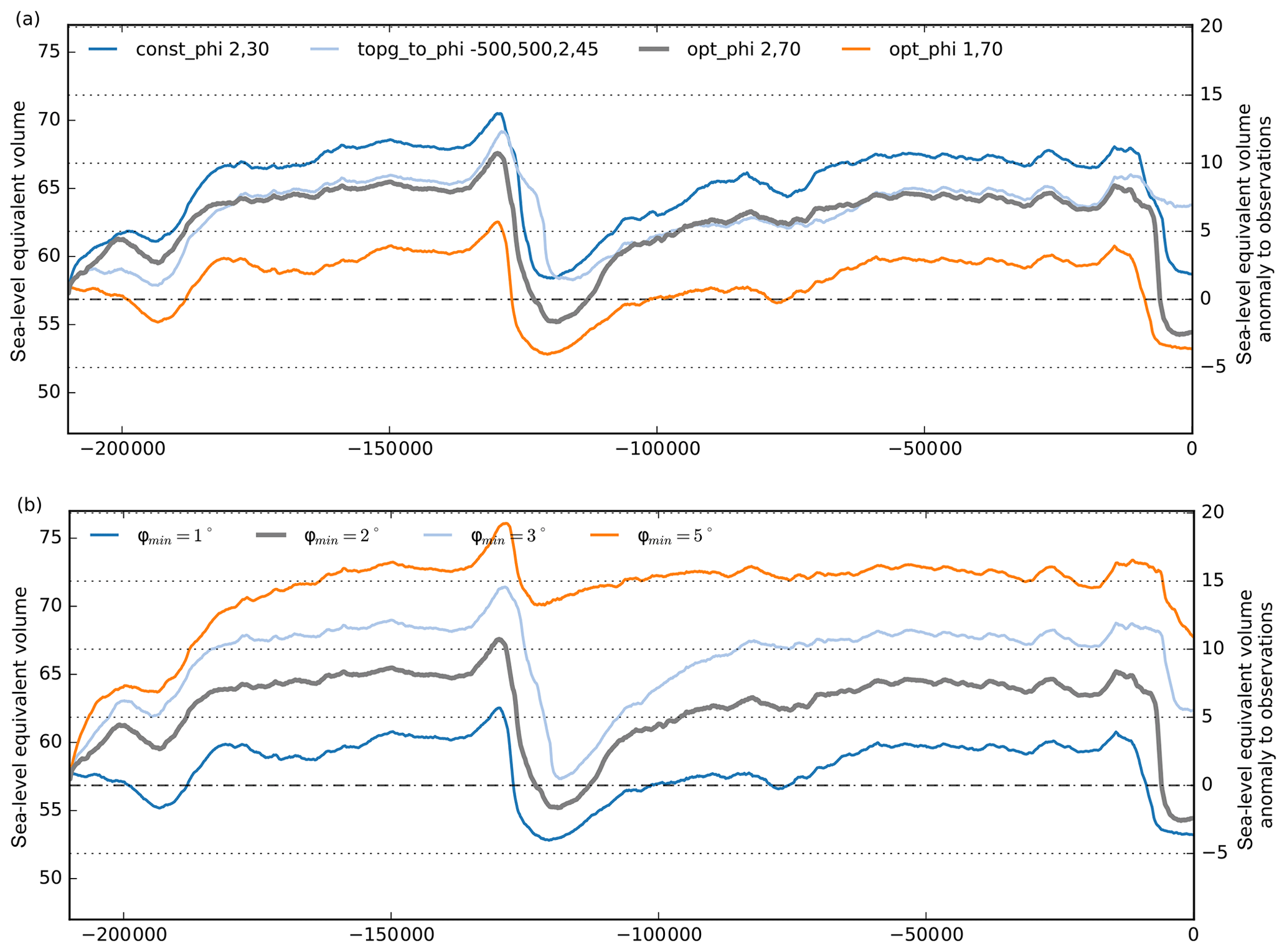
Figure 15Ice volume histories over two glacial cycles for different parameterizations of till friction angle. (a) For a spatially uniform ϕ (with 30∘ in grounded ice and 2∘ elsewhere; blue) and a till friction angle that is parameterized as function of the bed topography (light blue), the simulated ice volumes are generally larger than for the reference (grey), where ϕ is a result of the simple inversion technique. In those three cases the same minimal ϕmin was used. For a smaller ϕmin=1∘ we find generally smaller ice volumes. (b) The choice of ϕmin has strong influence on the reconstructed ice volume, with high till friction angles leading to more friction and hence thicker ice sheets. Within the plausible range from 1.0–5.0∘ we find up to 18 m SLE difference in simulated ice volume above flotation.
3.4.3 Subglacial hydrology
Till water distribution
The effective till water content in PISM's non-conserving hydrology scheme is a result of the balance between basal melting and a constant drainage rate (see Eq. 3). PISM's default drainage rate of 1 mm yr−1 is smaller than the basal melting in most of the grounded Antarctic Ice Sheet regions such that till saturates over time. Higher decay rates can effectively drain the till water in the inner ice sheet regions, which generally cause less-extended and more-confined ice streams, less ice discharge, and hence thicker ice sheets.
In transient glacial-cycle simulations, this relationship applies for both present-day climate conditions (see Fig. 16) and colder-than-present climates. A till water drainage rate of 10 mm yr−1 can cause up to 11 m SLE additional ice volume (light blue line in Fig. 17).
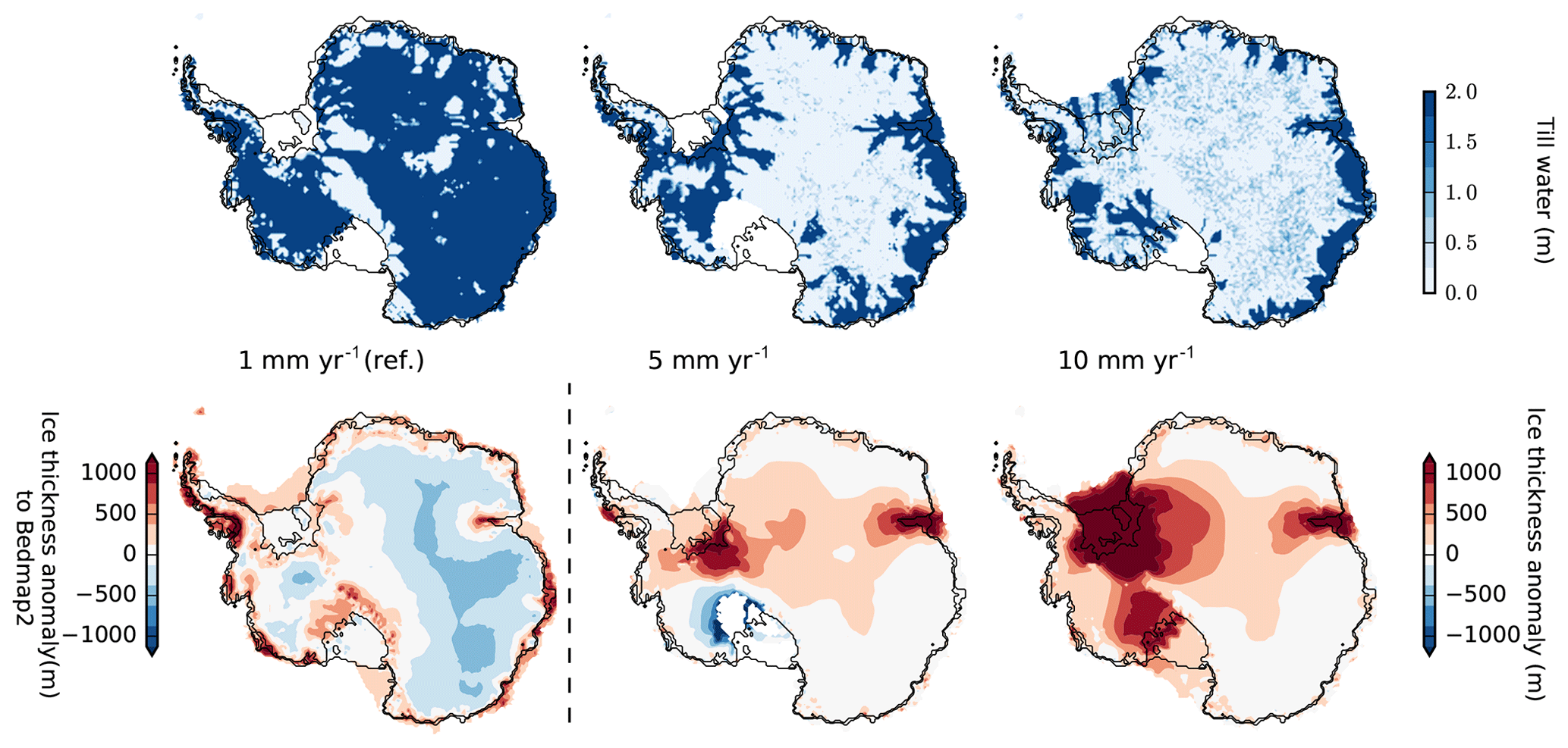
Figure 16Present-day result of glacial-cycle simulation, showing ice thickness anomaly in Bedmap2 (lower left) or in reference for different till water decay rates (from left to right: 1, 5 and 10 mm yr−1), causing different till water distributions underneath the ice sheet (upper row). For a reference decay rate of 1 mm yr−1 about 90 % of ice sheet's bed is saturated, while for 10 mm yr−1 saturated till is only found in the coastal regions and underneath the fast-flowing ice stream.
Another relevant aspect is the initial till water fraction on ocean beds that become grounded. PISM assumes that the grounding line advances into dry till area Wtill=0, where a till water layer can form over the following decades or centuries. If we assume a rigid till layer at the ocean floor instead, with , this affects grounding-line migration. We hence find slower growth of glacial ice sheet volume and much earlier deglaciation, while ice volumes are comparable to the reference case for present-day climate conditions (compare orange and grey line in Fig. 17).

Figure 17Simulation over two glacial cycles for different till water decay rates and for different fractions of the overburden pressure underneath the grounded ice sheet. (a) Higher decay rates than the reference value of Cd=1 mm yr−1 (grey) cause less-extended ice streams, less ice discharge and hence thicker ice sheets (blue and light blue). When assuming maximum till water fraction across ocean beds, grounding-line advance of marine glaciers is decelerated. Accordingly, we find a less-extended and thinner ice sheet at glacial periods, earlier retreat, but similar present-day results (compare grey and orange lines). (b) The critical fraction of the effective overburden pressure δ has strong influence on the reconstructed ice volume, particularly at glacial maximum, with high parameter values leading to more friction and hence thicker ice sheets. For the evaluated range of 2 %–8 % we find up to 12 m SLE difference in the ice volume above flotation.
Critical overburden pressure fraction
The effective pressure cannot exceed the overburden pressure, i.e., , while in the case of a saturated till layer (s=1), Eq. (2) yields a lower limit , with δ being a fraction of the effective overburden pressure at which the excess water will be drained into a transport system. As the maximum amount of till water is abundant in large portions of the grounded Antarctic Ice Sheet, the parameter δ scales the lower bound of the yield stress and hence affects the total ice volume above flotation considerably.
PISM's default δ value is 2 %, while for the reference simulation we use 4 %, which yields a better score in a basal parameter ensemble (Albrecht et al., 2020, Appendix A). For double δ, PISM simulations suggest that the glacial ice volume change to be almost double (see Fig. 17b). Also, for higher values of δ, the onset of deglaciation occurs earlier.
In our PISM simulations the Antarctic Ice Sheet responds to externally prescribed climatic forcings. In this section we choose reconstructions of Antarctic temperatures and sea-level variations, which implicitly incorporate the past climate response to changes in orbital configurations and atmospheric CO2 content. However, in this stand-alone mode no feedbacks of the ice sheet to the climate system are considered, but we discuss contributions of the climatic forcings to the volume evolution of the Antarctic Ice Sheet.
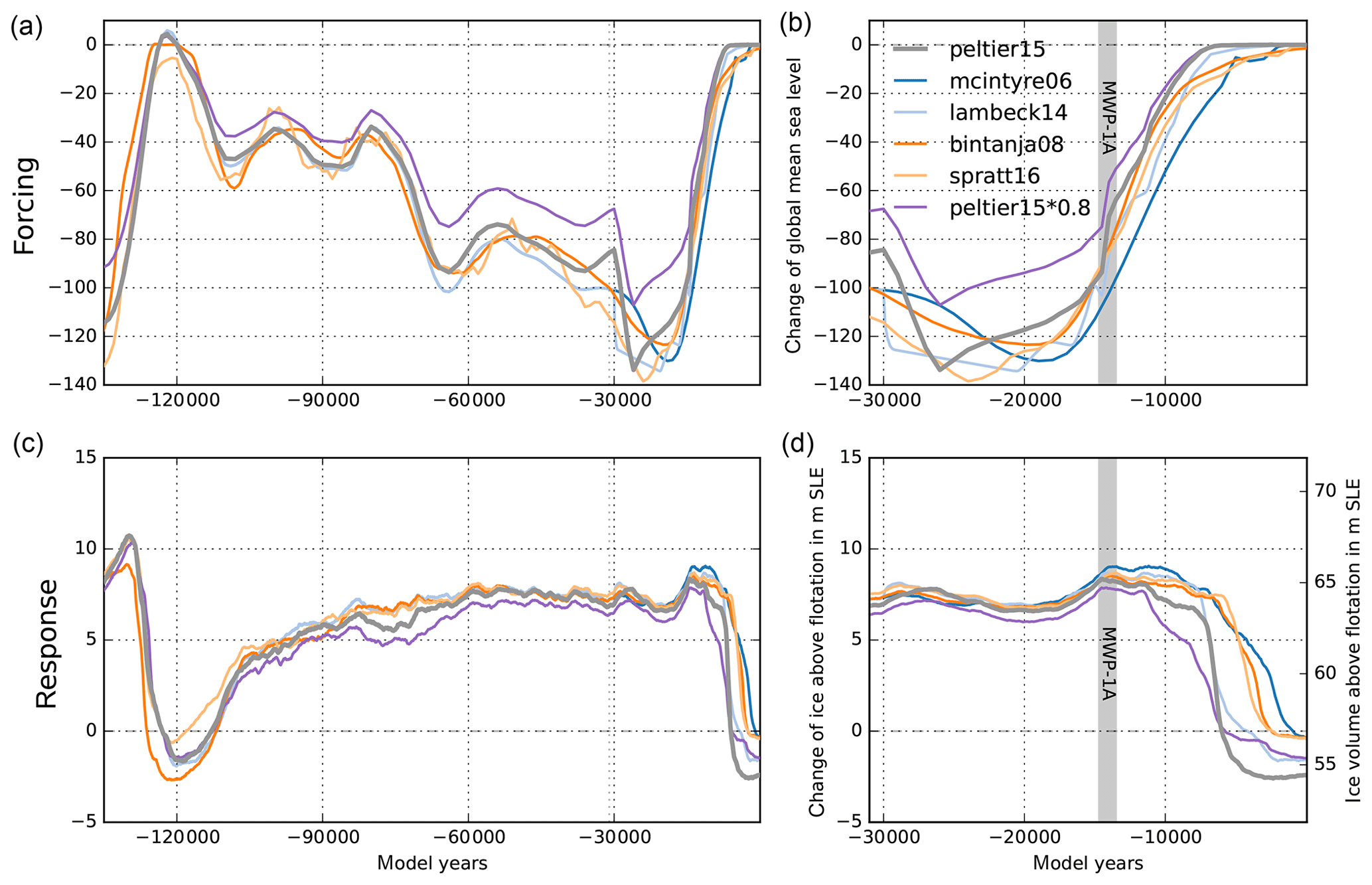
Figure 18Time series of reconstructed sea-level change over the last 135 kyr (a) and the last 30 kyr (b) by Stuhne and Peltier (2015), Imbrie and McIntyre (2006), Lambeck et al. (2014), Bintanja and Van de Wal (2008), and Spratt and Lisiecki (2016) and corresponding PISM-simulated sea-level-relevant ice volume anomaly relative to observations (Fretwell et al., 2013) in (c) and (d). In order to approximate the effect of self-gravitation we scaled the ICE-6G forcing (Stuhne and Peltier, 2015) by 80 %. For about 25 m higher sea-level stand at LGM we find almost the same modeled ice volume, while we find earlier but more gradual deglaciation (violet).
4.1 Sea-level forcing
The Antarctic Ice Sheet, particularly in its western part, rests on a bed below sea level with floating ice shelves attached. The location of the grounding line in PISM is solely determined by the flotation criterion (cf. H≤hf in Eq. 7) and therefore also by the current sea-level height zsl. Marine ice sheet dynamics are hence sensitive to changes in sea level, which has been 120–140 m lower than today at the Last Glacial Maximum. We neglect regional sea-level effects due to changes of the rotation of the Earth or due to self-gravitation, which can have locally a stabilizing effect on the ice sheet (Konrad et al., 2015). Instead, we consider global mean sea-surface-height reconstructions prescribed by the GIA model ICE-6G_C, which accounts for a changing surface area of the oceans (Stuhne and Peltier, 2015, 2017, courtesy Dick Peltier). To analyze the sensitivity of the model's response to the choice of the sea-level forcing, we compare our results to other reconstructions by Lambeck et al. (2014), Bintanja and Van de Wal (2008), Imbrie and McIntyre (2006), and Spratt and Lisiecki (2016). Focusing on the last deglacial period, the timing of sea-level rise onset in response to the melting of the northern hemispheric land ice masses varies by a couple of thousand years among the different sea-level curves (Fig. 18). For instance, the reconstruction by Stuhne and Peltier (2015) peaks already before 25 kyr BP, with around 130 m below present (grey), while the much smoother SPECMAP sea-level curve by Imbrie and McIntyre (2006) has a minimum around 18 kyr BP and a comparably late relaxation to the present-day sea level (blue).
The modeled Antarctic Ice Sheet response at the Last Glacial Maximum is rather unaffected by the choice of the sea-level forcing, while in contrast the ice volume at present varies by up to 2.5 m SLE (Fig. 18d). In particular, the meltwater pulse 1a (MWP1a; Liu et al., 2016) at around 14.35 kyr BP, with a global sea-level rise of 9–15 m or more within a few hundred years (see grey vertical band in Fig. 18), is well represented as a step in the sea-level curve in the reference forcing time series of the ICE-6G_C model. About 4 kyr after MWP1a, this triggers a comparably early and quick grounding-line retreat in the Ross and Weddell Sea embayment, where the large modern ice shelves begin to float.
If self-gravitational effects were accounted for within a sea-level model, the local sea-level anomaly at the grounding line would be reduced compared with the global mean. A scaling of the sea-level forcing by 80 %–90 % would mimic the first-order feedback of self-gravitation on grounding-line motion. Interestingly, neither the ice volume at LGM nor that at present is significantly affected, while the onset of deglaciation occurs earlier and with a lower rate (Fig. 18; violet line).
4.2 Surface temperature forcing
Varying surface temperatures drive ice flow changes on glacial timescales. In PISM we model the nonlinear thermo-coupling via a Glen-type flow law with a generalized form of the Arrhenius equation. More specifically, PISM's default flow law is the polythermal Glen–Paterson–Budd–Lliboutry–Duval law (Lliboutry and Duval, 1985; Aschwanden et al., 2012), where the ice softness depends on both the temperature and the liquid water fraction. Hence it parameterizes the (observed) softening of ice at pressure-melting temperature as its liquid fraction increases. Since vertical diffusion processes in the ice are rather slow, the corresponding response of the ice sheet to surface temperature anomalies occurs with a considerable delay of up to a few thousand years, involving a long-lasting memory for past events (cf. Sect. 1.3). On paleo-timescales PISM can use temperature reconstructions from ice cores based on deuterium isotopes, such as the EPICA Dome C ice core (EDC; Jouzel et al., 2007). This is a well-resolved time series over the last 803 kyr (EDC3 age scale), representative of the inner East Antarctic Ice Sheet. However, most of the ice-dynamical changes on glacial timescales occur in the marine regions of the West Antarctic Ice Sheet. The much closer WAIS Divide ice core (WDC) provides a highly resolved temperature reconstruction (Cuffey et al., 2016), but it spans only the last 67.7 kyr. As surface temperature forcing ΔT(t) we consider the WDC temperature anomaly with respect to the year 1950 CE added to the parameterized temperature field of Sect. 3.1. For model periods before 67.7 kyr the temperature anomaly of EDC applies (with respect to the last 1000-year average), with a small jump of 0.2 K, which is within the variability (see Fig. 19a and b). The EDC temperature reconstruction shows generally higher variability than the WDC reconstruction.
As expected, the Antarctic Ice Sheet volume responds in our simulations with a delay of several thousand years to the surface temperature forcing. The LGM minimum in surface temperature reconstructions happened around 22 kyr BP in the WDC data, while the largest ice volume is simulated at 14 kyr BP. The main temperature rise at WDC occurred between 18 and 12 kyr BP, contributing to initial deglaciation at around 12 kyr BP, with major retreat between 8 and 4 kyr BP in our reference simulation. At the EDC location the reconstructed temperature rise happened about 1 kyr later and with more variability, leading to a more gradual deglaciation between 12 and 2 kyr BP (Fig. 19; blue). Comparisons with other ice core temperature reconstructions, however, suggest a superimposed lapse-rate effect due to surface height change during deglaciation at the WDC location (Werner et al., 2018). This means that Antarctic temperature anomalies with up to −10 K at glacial maxima may be systematically overestimated (personal communication with Eric Steig). We thus also tested for a scaled temperature reconstruction from WDC with a LGM temperature of only 6 K below present (see light blue lines in Fig. 19). Interestingly, this weaker temperature forcing results in slightly thicker glacial ice volume (probably an effect of temperature-coupled surface mass balance; see Sect. 4.4) and delayed deglaciation.
We also tested for the influence of temperature variability on the simulated ice volume (Mikkelsen et al., 2018) and found slightly earlier initial retreat for the 500-year moving-average WDC temperature forcing. In contrast, for added white noise of 1.5 K variance, the present-day ice volume is more than 5 m SLE larger than in the reference (compare orange, light orange and grey lines in Fig. 19).
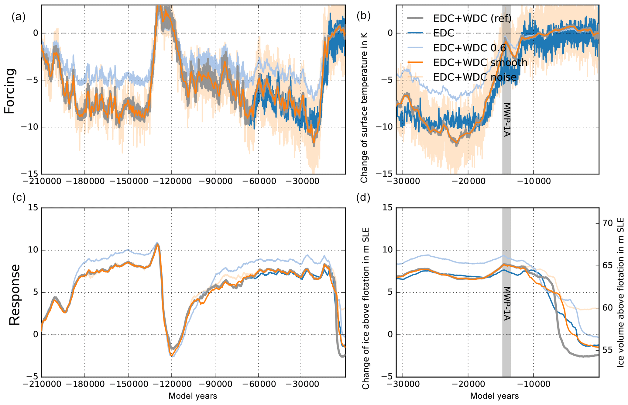
Figure 19Time series of PISM-simulated ice volume above flotation relative to observations (Fretwell et al., 2013) over last 135 kyr (c) and last 31 kyr (d) forced with different surface temperature reconstructions (a, b) at WDC (Cuffey et al., 2016, grey) and EDC (Jouzel et al., 2007, blue), leading to different ice volume histories, particularly during deglaciation period. The WDC temperature reconstruction scaled by 60 % causes 2 m SLE larger glacial ice volume and slower deglaciation (light blue). When WDC temperature reconstruction is smoothed, we find a slightly earlier initial retreat (orange), while added white noise leads to higher ice volume at present (light orange).
4.3 Ocean temperature forcing
Sub-shelf melting in PISM is calculated via PICO (Reese et al., 2018) from salinity and temperature in the lower ocean layers on the continental shelf (Schmidtko et al., 2014) averaged over 18 separate basins adjacent to the ice shelves around the Antarctic continent. While salinity change over time in the deeper layers is neglected in this study, the ocean temperature responds with some delay to changes in the global mean temperature. We analyzed simulations with the coupled climate model ECHAM5–MPIOM over more than 6000 years following a 4-fold increase in CO2 forcing (courtesy Li et al., 2012) and identified the anomaly in global mean temperature, in Antarctic temperature (south of 66∘ S) and in Antarctic ocean temperature at depth levels between 500 and 2,500 m. After a response time of about 3000 years the ocean temperature stabilizes at about fo=0.75 of the global mean anomaly, while Antarctic surface temperature anomaly is amplified by a factor of 1.8 (see Fig. 20a). As we intend to estimate ocean temperature change from ice surface temperature change reconstructed from ice cores, we could have fitted the response function directly from the Antarctic mean surface temperature in the climate model data. But we prefer to use a more general relationship, defined as response to global mean temperature change, which makes it easier to compare to other approaches. We found that, for the timescales considered here, Antarctic surface temperatures respond almost linearly with global mean temperature change. We therefore assume in the analysis that both time series are interchangeable except for the inferred amplification factor.
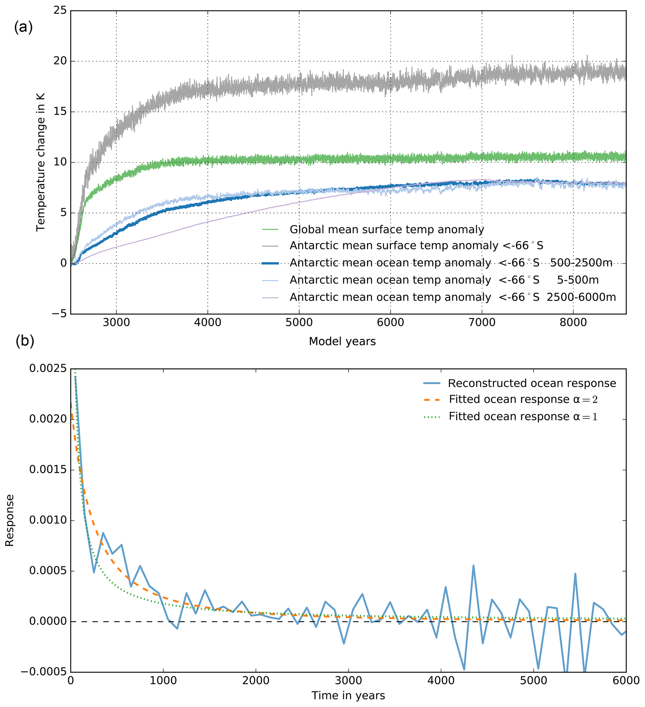
Figure 20Climate model data and response function analysis – (a) global mean temperature (green); Antarctic mean temperature south of 66∘ S (grey); and ocean temperature averaged over upper 500 m (light blue), intermediate (500–2500 m; blue) and deeper layers (below 2500 m; violet) of the MPIOM model coupled to ECHAM5 forced by a CO2 quadrupling within 140 years (Li et al., 2012). (b) Reconstructed response function R(t) (blue) with fitted function R*(t) (orange dashed) as in Eq. (14). For comparison the fit function with α=1 (green dotted) is shown.
Using linear response theory (Winkelmann and Levermann, 2013) and assuming the global mean temperature anomaly ΔTGM(t) via a convolution integral related to the ocean temperature as
we reconstruct a response function R(t) and a corresponding fit function with (see Fig. 20b), which vanishes beyond the typical response time τr. For α=2 and with an integration constant in the numerator, such that
is valid, this yields
The inferred response fit function convoluted with a given time series of global mean surface temperature anomaly (or here with the scaled ice core temperature reconstruction) hence provides an estimate for the corresponding change in ocean temperature at intermediate depth. Figure 21 shows the estimated ocean temperature anomaly curve (blue) with some delay with respect to the WDC surface temperature reconstructions (grey; Cuffey et al., 2016), here for easier comparison also shown scaled by % (purple). The WDC likely better reflects the ocean conditions in the widely marine West Antarctic Ice Sheet than the EDC, which is located in central East Antarctica (Jouzel et al., 2007).
The inferred ocean temperature time series is comparably smooth with a resolution of 500 years and serves PICO as ocean temperature forcing. A comparison to reconstructions with a general circulation model (GCM) in the TraCE-21ka project (Liu et al., 2009)3, suggests that short warming periods above the present level could have occurred at intermediate depth, e.g. during Antarctic Cold Reversal (ACR) at around 14 kyr BP, which cannot be adequately resolved with our approach. The GCM ocean data are bounded below by the pressure-melting point. As negative ocean temperature anomalies can result in unphysical values below the pressure-melting point, we leave it to the PICO module to assert this lower bound such that melting vanishes and overturning circulations halts accordingly. As a consequence, ocean forcing becomes irrelevant for much-colder-than-present glacial climates. The parameterization presented here assumes that ocean water masses at depth below 500 m can access ice shelf cavities and induce melting, which is certainly very simplified regarding the complex bathymetry and flow patterns around Antarctica. Also, we used data from a simplified sensitivity experiment with ECHAM5–MPIOM, for a warmer-than-present climate, which implies various model uncertainties. We also had to make assumptions about a suitable response function, which is fitted to model data that are averaged over certain regions and ocean depths, implying further uncertainties.
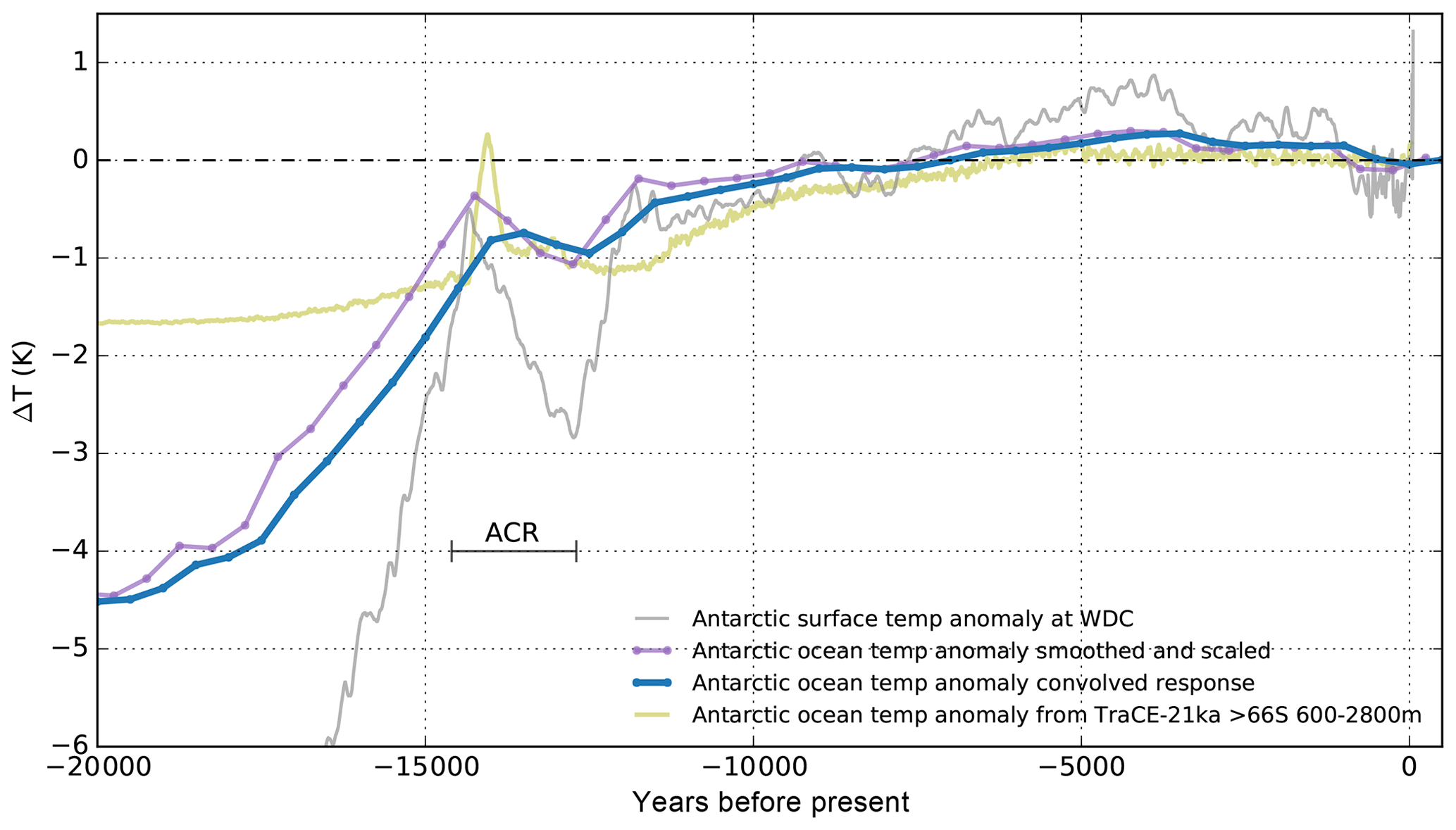
Figure 21Response of the intermediate ocean temperature (blue) to surface temperature anomaly, as reconstructed from WDC (Cuffey et al., 2016, grey line), assuming a polar amplification factor of 1.8 and an equilibrium ocean scale factor of 0.75, as identified in climate model analysis for a warming scenario. Convolution yields a delayed response (blue) with respect to the forcing, shown here as scaled curve (violet), with dots indicating bins of 500-year means. The time series includes the Antarctic Cold Reversal (ACR) of 14.6–12.7 kyr BP (Fogwill et al., 2017). For comparison, GCM ocean temperature anomaly is shown (in olive), as reconstructed by TraCE-21ka (Liu et al., 2009), for the mid-ocean depth 600–2,800 m and south of 66∘ S.
Transient PISM simulations reveal a delayed response of the ice volume to the ocean temperature forcing, with the main deglaciation occurring when temperature anomalies reach almost present-day levels (Fig. 22; cf. upper and lower panels). When we directly apply the smoothed and scaled surface temperature forcing as PICO forcing, we still get very similar results but a slightly earlier retreat (orange). Simulations reveal that the power of the response function (cf. Fig. 20b) is of minor relevance to the ice sheet's response (compare grey and blue lines). Also the amplitude of cooling at glacial stage, here scaled by 60 % (light orange), shows only little change in the simulation results. If the ocean forcing is related to the EDC temperature reconstruction (see Sect. 4.2) we find a later warming and hence delayed deglaciation (light blue). Ocean forcing likely plays a key role in warmer-than-present climates. However, we do not see this effect in our simulations during the Last Interglacial. Although ocean temperatures rise by more than 1 K above the present we find similar ice volumes to the present in all our simulations. Precipitation scaling and the till properties seem to play an important role in stabilizing WAIS and preventing collapse. However, a thorough investigation of necessary model settings for WAIS collapse during the LIG would fill a separate study.
As we employ an anomaly forcing, which becomes near zero at present, the modeled modern ice sheet configurations are rather independent of the applied ocean temperature forcing (except for EDC, which is generally colder through the Holocene). Also, there is literature suggesting periods of decoupled ocean and surface temperature evolution (e.g., ACR) with strong potential effects on the ice sheet deglaciation. Appendix A1 provides an estimate of the effect of intermediate ocean warming events from a simple perturbation analysis with PICO.
4.4 Precipitation forcing
Continental-scale precipitation change is closely related to temperature change. While colder temperatures lead to higher effective ice viscosity and hence to slower ice flow and larger ice masses, they also lead to dryer conditions and hence to less ice mass accumulation. This effect is based on the Clausius–Clapeyron relationship, which suggests higher atmospheric moisture capacity and hence more accumulation in a warmer atmosphere. On average over the Antarctic continent, the analysis of ice core and modeling data suggest a linear scaling relationship between precipitation and temperature change of % K−1 (Frieler et al., 2015). In PISM simulations, precipitation forcing P(t) is coupled directly to the temperature forcing ΔT(t) (Sect. 4.2) using an exponential relationship (Ritz et al., 1996; Quiquet et al., 2012, Eq. 2), which scales the present-day mean precipitation field P0 as
The exponential function is hence compatible with the precipitation lapse correction (Eq. 11), and it allows for easier comparisons with other studies that use power law relationships, e.g., with for Pollard and DeConto (2009). In fact, precipitation change depends very much on the Antarctic region. In our simulations we use a combination of temperature reconstructions from the EDC and WDC for ΔT(t) (see Sect. 4.2). Compared to the Antarctic mean value, the study by Frieler et al. (2015) suggests slightly higher values at core locations of % K−1 and % K−1, respectively. In East Antarctica estimates of the linear precipitation scaling factor tend to be slightly higher than in West Antarctica.
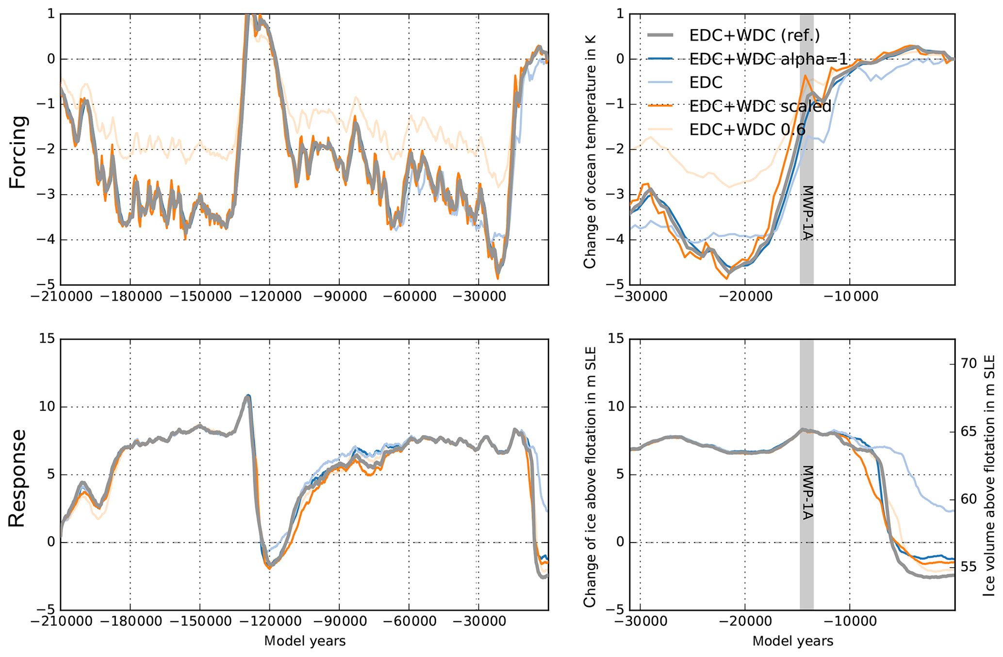
Figure 22Sensitivity of transient ice volume above flotation to varied ocean temperature forcing. Reference simulation (grey) is based on EDC + WDC surface temperature with fit response function of power α=2. The resulting ice volume change is similar for a fit response function with power α=1 (blue). Even if ocean temperature forcing responds directly to the scaled surface temperature anomaly (orange), the resulting effects on ice volume are comparably small. If a different surface temperature reconstruction is used, here from EDC with α=2 (light blue), we find, in response to a later warming signal, delayed deglaciation. If the amplitude of WDC surface temperature anomalies were 40 % lower (light orange), this would have only negligible effect on the modeled ice volume.
In glacial periods with much colder temperatures of K, an exponential precipitation change with fp=7–9 % K−1 yields 50 %–60 % less precipitation when compared to modern times. Without any temperature-scaled precipitation change, our simulations suggest up to 7 m SLE thicker ice sheets at the Last Glacial Maximum (cf. grey and light blue line in Fig. 23). The reference value of 7 % K−1 precipitation change corresponds to more than 50 % dryer conditions than the present and about 3–4 m SLE less ice volume than for 5 % K−1 (cf. grey and blue line). Reconstructions of precipitation at ice core sites, e.g., at WDC (Buizert et al., 2015; Fudge et al., 2016), reveal precipitation changes relative to present of up to −60 % during LGM and up to 25 % more precipitation through the Holocene. Figure 23 shows the corresponding transient effects of reconstructed precipitation forcings on the ice sheet's volume above flotation (orange line). The additional accumulation during the Holocene at WDC prohibits deglaciation and causes a modern ice sheet configuration that is more than 10 m SLE larger. However, the reconstructed signal at WDC may be biased to some extent from a lapse-rate effect due to surface elevation changes during deglaciation (personal communication with Eric Steig). Interestingly, we find a similar ice volume response when applying no lapse-rate correction for changing surface elevation (as described in Eq. 11), which also diminishes deglaciation (light orange in Fig. 23; for the same precipitation forcing as the reference). The simulations hence suggest that the precipitation scaling parameter fp is highly relevant to the ice sheet's extent at glacial maximum and will be considered to be ensemble parameter PREC in Albrecht et al. (2020).
4.5 Combined effects of climatic forcings in glacial-cycle simulations
In our simulations with PISM the climatic forcings described above (Sect. 4.1–4.4) have different effects on the Antarctic Ice Sheet evolution at different periods. Both temperature and sea-level forcing reveal a periodic signature not only of the dominant 100 kyr orbital cycle but also with smaller amplitudes of the higher-frequency cycles, e.g., Marine Isotope Stage 3 (MIS 3) around 57 kyr BP (Weichselian High Glacial) or the MIS 2 at the Last Glacial Maximum around 29 kyr BP (Lisiecki and Raymo, 2005). For glacial-cycle simulations, sea-level forcing has the strongest effect on the ice volume, as it alone can trigger a larger glacial ice volume than in the reference simulation (see Fig. 24b; orange and grey). However, the rising sea level during deglaciation alone induces only little ice sheet retreat. When sea-level forcing is turned off, the other forcings balance each other out such that ice volume remains approximately at modern level through glacial periods (Fig. 24c). Also surface temperature forcing alone (Fig. 24b; blue) can produce glacial volumes of similar extent to the sea-level forcing. But if surface temperatures remain at modern levels, the other forcings can still produce a glacial maximum volume that is only 3 m SLE lower than the reference. In our simulations, surface temperature anomalies also drive changes in ocean temperature and precipitation. Ocean temperature forcing has only little effect on glacial extent, but it influences the onset of deglaciation (light orange). Without ocean forcing the interglacial (and modern) ice volume is hence up to 7 m SLE larger than in the reference (Fig. 24c). While sea-level and temperature forcings cause a growth of ice sheets at glacial climates, precipitation forcing has the opposite effect (Fig. 24; light blue). Without precipitation forcing the Antarctic Ice Sheet can reach glacial extents of up to 7 m SLE above the reference (coupled to the surface temperature forcing with fp=7 % K−1). This effect of the precipitation forcing for glacial climates also explains why the individual responses to the sea-level and the surface temperature forcing exceed the reference ice volume by about 3–4 m SLE, in which all four forcings are superimposed.
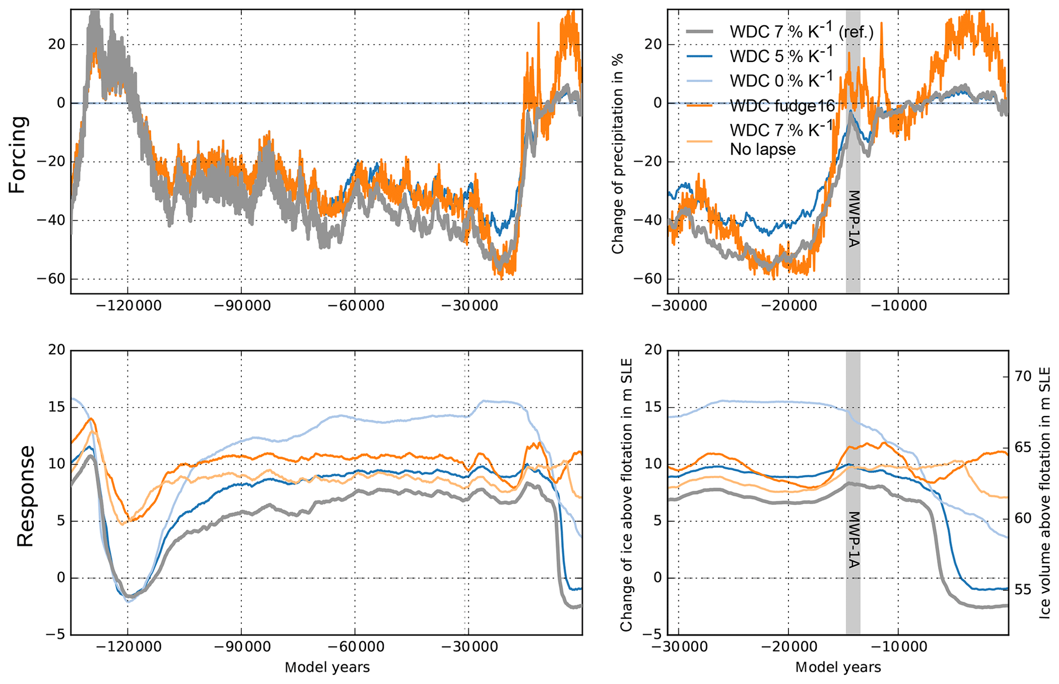
Figure 23Sensitivity of transient ice volume above flotation to varied precipitation forcing. Grey curve is the reference, with an exponential scaling factor of 7 % K−1 with respect to WDC temperature reconstruction (Cuffey et al., 2016). Ice volume is slightly larger for 5 % K−1 (blue) and much larger without precipitation forcing (light blue). Deglaciation is prohibited when using WDC accumulation reconstruction (Fudge et al., 2016) with additional accumulation during Holocene (orange). A similar effect is seen when no lapse-rate correction is applied for the precipitation (light orange).
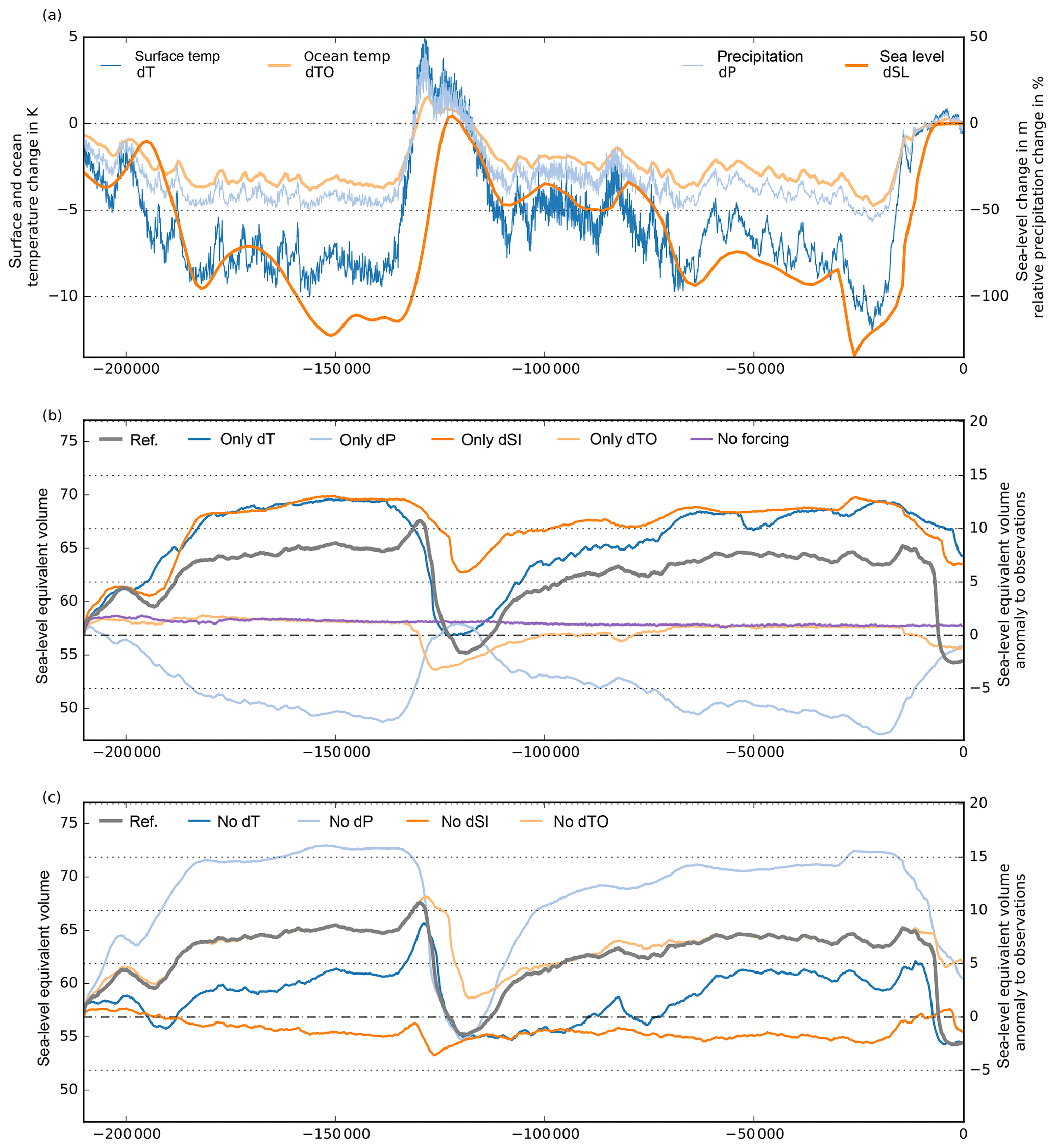
Figure 24Antarctic Ice Sheet volume above flotation for combinations of surface temperature, ocean temperature, sea-level and precipitation forcings (a), as defined in previous sections. (b) The ice sheet's response to individual forcings (or constant equilibrium conditions in purple) or (c) in the absence of one of the forcings, compared to the reference simulation (with all forcings combined; in grey). Sea-level forcing (orange) and surface temperature forcing (blue) have the strongest effects: each alone can cause larger glacial ice volume than in the reference simulation. However, each alone cannot initiate effective glacial retreat during modern climate. In contrast, ocean temperature forcing (light orange) has no effect on glacial volume, but it amplifies deglaciation. Precipitation forcing (light blue) counteracts sea-level and temperature forcings in glacial climates.
Our results are in line with another recent study using the PSU-ISM ice sheet model. In this study, they also find a dominance of atmospheric and sea-level forcing on the Antarctic ice volume over the last four glacial cycles (Tigchelaar et al., 2019), which together drive glacial–interglacial ice volume changes of 12–14 m SLE, while ocean temperature forcing is almost negligible, also during interglacials. Here, we do not want to go into the details of this study, which uses a comparably coarse output of an Earth system model of intermediate complexity for the atmospheric and ocean forcing instead of scaling with ice core temperature reconstructions. As a key result, Tigchelaar et al. (2019) find much smaller individual ice volume changes, which amount to less than half of the full ice volume response. In our simulations, however, the individual response to sea-level forcing (and surface temperature forcing) and the sum of all individual forcings exceed the combined response. This is partly due to the fact that precipitation forcing (up to 50 % less during glacial climate) provides a strong negative effect on the ice volume in the full-forcing case, which seems to be weaker in the “atm” forcing in Tigchelaar et al. (ca. 15 % in Fig. 8; 2019). If we consider the LGM and present-day state to be rather stable states, a certain perturbation threshold must be crossed to initiate the (nonlinear) transition (Termination I) into the other state. In our simulations this threshold can be reached with individual forcings, while in the other study the combined superposition is required.
Table 2Sensitivity (mean and standard deviation) of simulated ice volume at Last Interglacial (LIG), Last Glacial Maximum (LGM) and present day (PD) for varied input datasets and model parameters (some of which are already indicated in Table 1), and the used reference value. Selected ensemble parameters for each category are bold: VISC and PPQ are more relevant to deglacial and present WAIS dynamics, and ESIA and PREC are relevant rather to EAIS dynamics. Asterisk indicates a different PISM version used.
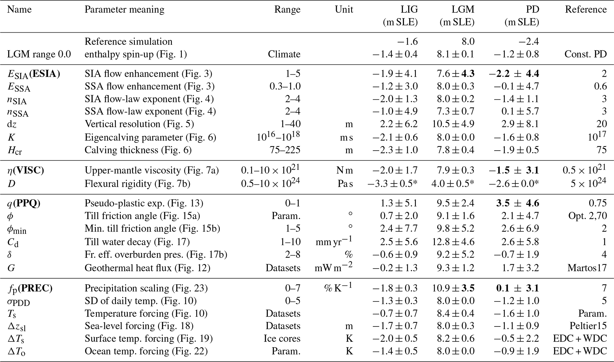
In this study we ran PISM simulations of the Antarctic Ice Sheet over the last two glacial cycles. In the following we summarize the main findings of our sensitivity analysis with regard to the impact of different model parameter settings, boundary conditions and climate forcing choices on the evolution of the ice sheet volume. Table 2 provides a brief overview over tested parameter ranges and statistics on the results. Differences in ice volume above flotation were characterized for specific periods, in particular for the Last Glacial Maximum (LGM) and for the present, while at the Last Interglacial the modeled ice volumes were generally around 1 m SLE lower than the present. During deglaciation, small perturbations can be amplified, causing a strong divergence in the ice sheet response. We estimated the amount of model-intrinsic uncertainty to be around 1 m SLE for present-day climate conditions and much smaller for glacial conditions. Hence, simulated changes in interglacial ice volume due to variations in parameters or boundary conditions are considered “significant” when larger than this intrinsic uncertainty. Within this uncertainty range, we found consistent results for the reference horizontal grid resolution of 16 km and finer, while we did not find convergence for much higher vertical resolution of up to 1 m at the base. Regarding ice-dynamical parameters, we found the largest sensitivity in present-day ice volume for variation in the SIA and SSA flow enhancement factors as well as for the SSA flow-law exponent. The ESIA flow enhancement also shows high sensitivity at LGM.
Processes at the interface of ice and bedrock are highly uncertain. For the application of different geothermal heat-flux maps, we found the largest sensitivities for the present-day state with more than 3 m SLE standard deviation. Basal friction in PISM is associated with various hydrological and microscale processes. Geological properties of the basal substrate expressed as till friction angle are a key parameter here. We presented an optimization algorithm for till friction angle distribution to minimize the misfit to modern grounded ice thickness (Sect. 3.4.2). However, simulated ice streams were less confined than with a piecewise-linear parameterization dependent on bed topography. Modern ice shelf regions were covered by grounded ice in glacial climates, where till properties are weakly constrained. A variation in the minimal till friction angle caused a simulated ice volume range of up to 8 m SLE. Also variation in the hydrological model parameters shows large sensitivities. Variations in till water decay rate and of the critical fraction of effective overburden pressure revealed additional considerable uncertainties of up to 6 m SLE each. Variation in basal sliding from plastic till deformation to linear sliding in terms of the sliding exponent PPQ also yields an ice volume uncertainty of more than 5 m SLE, in particular at the LIG and present day. The basal model components are consequently the least constrained and most sensitive parts in PISM glacial-cycle simulations.
Within the coupled Earth model, an increase in mantle viscosities by 2 orders of magnitude caused slower ice sheet growth but faster deglaciation. We found that the effect of changing global mean sea-level height and bed topography as a result of the glacial isostatic adjustment represents a relevant feedback on grounding-line migration that can amplify the ice sheet growth for glacial climates by more than 5 m SLE. In contrast, we identified a comparably low sensitivity of glacial ice volume to variations in the elastic part of the Earth model, expressed via the parameter for flexural rigidity.
In our study we presented a parameterization for the ice surface temperature fitted to modern reanalysis data, which accounts for changes in geometry and that can be easily used in combination with the PPD scheme (Sect. 3.1). Variation in PDD parameters or the consideration of more realistic temperature distributions from a regional climate model or reanalysis data have only an insignificant effect on the simulated ice volume history. In order to run glacial-cycle simulations we prescribed past external climatic forcings for sea level, surface air and ocean temperatures as well as for precipitation. For different reconstructions of sea-level and temperature forcing we found rather low ice volume sensitivities of below 1 m SLE at LGM and up to 2 m SLE at present. A sensitivity of more than 3 m SLE is found for the precipitation forcing when the scaling parameter PREC is varied. Ocean temperature change is modeled as a delayed response to changes of reconstructed air temperatures (Sect. 4.3). The tested sensitivity to different response functions and air temperature reconstruction may not cover the full range of oceanic uncertainties, in particular for deglaciation and warmer than present climates. Further sensitivity experiments with a focus on deglacial grounding-line sensitivity are discussed in Appendix A. Sea-level forcing is the most dominant forcing at play together with surface air temperature forcing, as each alone could trigger ice volume growth of more than 12 m SLE above the present at the Last Glacial Maximum. If no sea-level forcing were applied, temperature and precipitation forcing would balance each other out and the Antarctic Ice Sheet would remain at the modern configuration even for glacial climate conditions. However, in all simulations retreat occurred after MWP1a.
From the discussed model settings and boundary conditions, we select a total of four relevant parameters covering the different sections: “Ice sheet and Earth model parameters” (Sect. 2), “Boundary conditions and input datasets” (Sect. 3), and “Climatic forcing” (Sect. 4). Regarding the climatic forcing, we identified the precipitation change rate PREC as the most relevant uncertain parameter within the range of 2% K−1–10% K−1. For the Earth model the upper-mantle viscosity VISC was selected within the range of 0.1–10×1021 Pa s, while for the basal friction model the sliding exponent PPQ within the range of 0.25–1.0 was chosen. Finally, we determined the ESIA enhancement factor within the range of 1–7 to represent the vast uncertainty of the internal ice-flow dynamics on glacial-cycle timescales. While ESIA and PREC are more relevant to the LGM configuration of the Antarctic Ice Sheet, VISC and PPQ determine the timing and rate of deglaciation to the present-day configuration and are hence in particular relevant to the West Antarctic Ice Sheet. These parameter ranges define the dimensions of the parameter ensemble, which is presented and analyzed in the companion paper (Albrecht et al., 2020).
We have shown that PISM can be a powerful tool for paleo-simulations of Antarctic Ice Sheet evolution if ice sheet modelers take identified key uncertainties regarding model parameterization and forcing choices into account.
A1 Ocean forcing pulse at Antarctic Cold Reversal
Recent studies of coupled ice sheet and ocean dynamics (e.g. Golledge et al., 2014; Fogwill et al., 2017) suggest the idea of a positive feedback mechanism causing episodes of accelerated ice sheet recession as result of enhanced sub-shelf melt, in particular in an ocean warming event during the Antarctic Cold Reversal (ACR) coincident with meltwater pulse 1A (MWP1a). For comparably small changes in ocean forcing (≈0.25 K) Golledge et al. (2014) find a 3-fold mass loss from the Antarctic Ice Sheet (up to 6 mm yr−1). We ran a similar sensitivity experiment with an additional ocean temperature forcing of 1 and 2 K, causing enhanced sub-shelf melt via the PICO module. This range covers the anomaly found in GCM ocean temperature reconstructions from TraCE-21ka (Liu et al., 2009), averaged over 600–2,800 m depth and south of 66∘ S.
Compared to our reference run with only 0.25 m SLE contribution during the period of two millennia (grey), we detect enhanced melt during ACR (see grey bar and dotted vertical lines in Fig. A1) with a change in volume above flotation of 0.5 m SLE (blue) and 1.6 m SLE (orange) in the two sensitivity experiments, which corresponds to a mean sea-level contribution rate of 0.25 and 0.82 mm yr−1, respectively. Even though the ocean temperature forcing in the sensitivity experiments exceeds present-day level (with melt rates in the Ross and Weddell Sea above 1 m yr−1), its effect on ice volume seems comparably small, as grounding lines extend to the edge of the shallow continental shelf with rather small ice shelves attached. Accordingly, PICO responds with less overturning and melt as it would for a modern configuration of the Antarctic Ice Sheet and ice shelves. The sensitivity experiments with additional ocean temperature forcing early in the deglaciation phase show a more gradual ice volume retreat later in the Holocene and a 1–2 m SLE larger present-day ice volume.
A2 Grounding-line sensitivity
It remains an open question how much Antarctic deglaciation contributed to the MWP1a. A time series of well-dated sediment data of iceberg-rafted debris (Weber et al., 2014) suggest that the main retreat of the Antarctic Ice Sheet occurred at 14.6 kyr BP, synchronously with MWP1a, while the RAISED consortium concluded on a later retreat with a relatively small Antarctic contribution to MWP1a (Bentley et al., 2014). However, in our reference simulation the main retreat does not occur before 10 kyr BP. From our sensitivity experiments we can identify relevant model parameters and boundary conditions that affect the stability of the grounding line and hence the onset of the last deglaciation.
In PISM the location of the grounding line is determined by the flotation condition (cf. H=hf in Eq. 7), while at the same time it affects the overall stress balance and hence the ice sheet evolution. PISM simulates sub-grid basal friction according to interpolated grounding-line location between grounded ice sheet and floating ice shelf (Gladstone et al., 2010). Hence, grounding-line migration can be reasonably well represented in PISM (compared to full Stokes), even for coarse resolutions (Pattyn et al., 2013; Feldmann et al., 2014). The sensitivity of grounding-line motion also depends on applied boundary conditions. The availability of subglacial or sub-shelf meltwater in the vicinity of the grounding line may enhance ice flow or thinning, respectively. These model choices can induce some additional uncertainty, as has been indicated in Golledge et al. (2015).
Saturated till at the grounding line hampers grounding-line advance and amplifies grounding-line retreat (see Fig. A2; orange and light orange vs. grey). A more slippery grounding line, as has often been enforced in PISM simulations in previous studies (e.g. Golledge et al., 2015), appears to have a similar effect to the model improvement described in Sect. 3.4.5. Both show slower ice sheet growth and much earlier deglaciation from a less-extended glacial state. PISM can interpolate basal melt across the grounding zone boundary using the same interpolation scheme as for the basal shear stress (Sect. 1.1). In the reference simulation, the interpolation has been not applied correctly such that the effect of basal melting as calculated from PICO was underestimated. We find earlier deglaciation from a similar glacial state as in the reference simulation, when the melt interpolation is not applied or applied correctly4; blue and light blue in Fig. A2, respectively). Be aware that PICO melt rates are only defined underneath the ice shelf, and interpolation to the grounded ice sheet may jeopardize energy and mass conservation within PICO.
Another aspect that can potentially affect till water content and hence sliding in ice-stream regions is related to the temperate ice thermal conductivity ratio. This parameter is used to simulate a physical jump condition in the enthalpy gradient for temperate ice at the base such that the energy at the base is balanced by the basal melting (Kleiner et al., 2015). In the reference simulation we use a very low temperate ice thermal conductivity ratio of , as suggested by Kleiner et al. (2015). However, this ratio does not seem to affect the cold-temperate transition surface and hence the ice volume history in PISM much, even when varied over 4 orders of magnitude (default value CR=0.1; see light orange line in Fig. A2).
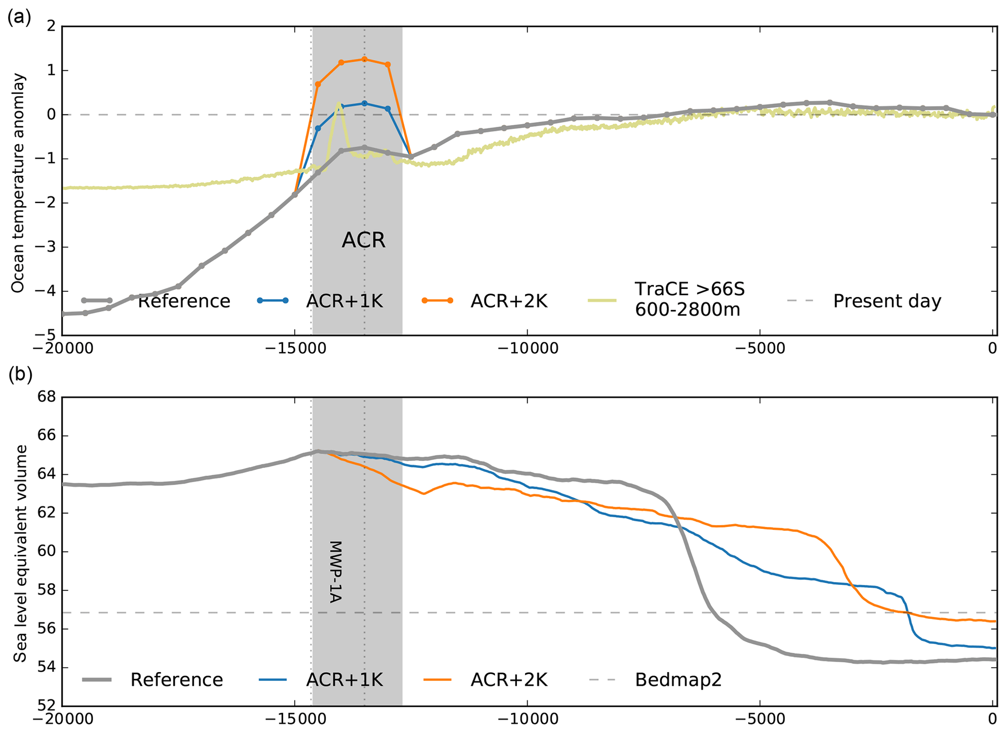
Figure A1Simulation over two glacial cycles (only last 20 kyr shown here) with different ocean temperature forcing, increased here by 1 or 2 K in the 2-millennium phase (14.6–12.7 kyr BP) of the ACR after MWP1a (a). Within this range, for comparison, the reconstructed GCM ocean temperature data from TraCE-21ka are shown as average over 600–2800 m depth and south of 66∘ S (green). The additional melt causes a doubling or even 6-fold increase in early ice volume losses, respectively, but most of the ice sheet retreat is somewhat delayed (b).
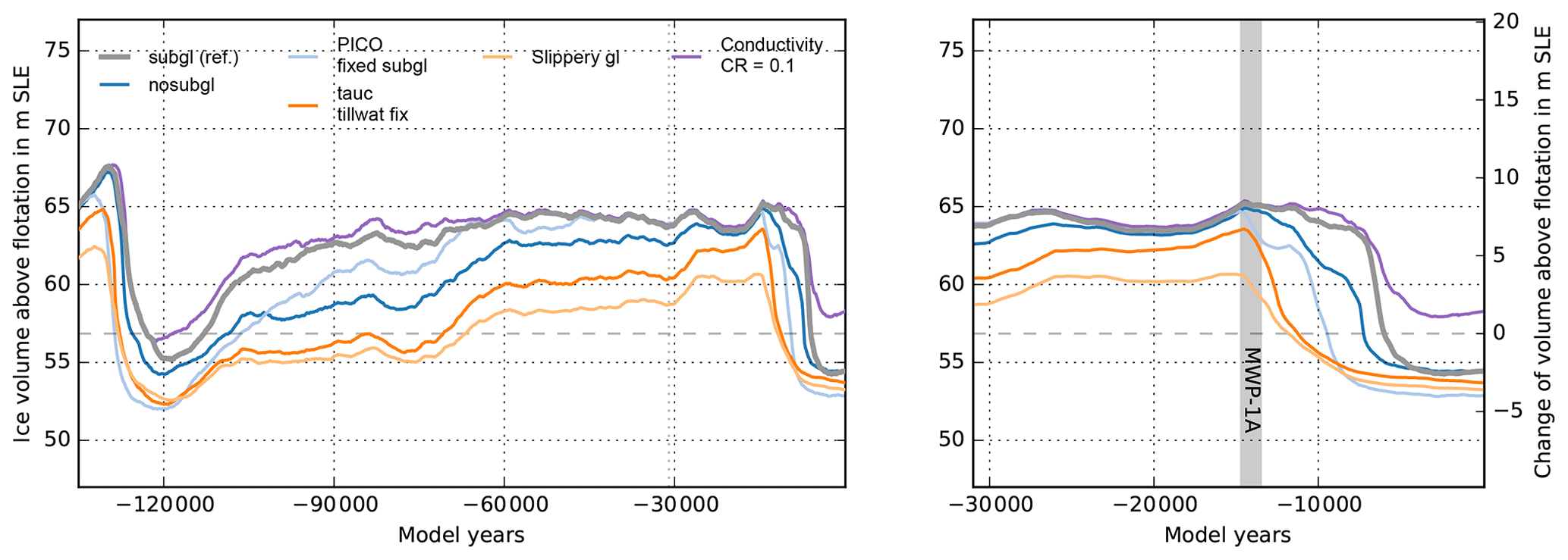
Figure A2Sensitivity of transient ice volume above flotation to varied conditions at the grounding line. Grey curve is the reference with applied sub-grid basal shear stress and old basal melt interpolation, which generally underestimates melting at the grounding line. Without basal melt interpolation (blue) or with fixed basal melt interpolation (light blue), deglaciation occurs earlier than in the reference, while glacial maximum extent is comparable. Glacial ice sheet growth is even slower for enforced saturated till conditions along the marine sections of the grounding line, landward (orange) or on the ocean side of the grounding line (light orange). The much higher sensitivity of the ice sheet volume to oceanic forcing yields a smaller glacial ice volume and much earlier deglaciation. The effect of variation in the temperate ice conductivity ratio over 4 orders of magnitude has only little effect, with slightly larger interglacial ice volumes for larger ratios (purple).
The PISM code used in this study can be obtained from https://doi.org/10.5281/zenodo.3574032 (Albrecht and PISM authors, 2019); most model improvements have been merged into the latest PISM development at https://github.com/pism/pism (last access: 27 January 2020; The PISM authors, 2020a). PISM input data are preprocessed using https://github.com/pism/pism-ais (last access: 27 January 2020; The PISM authors, 2020c). Results and plotting scripts are available from https://doi.org/10.1594/PANGAEA.909727 (Albrecht, 2019a).
Movie of reference PISM simulation of the Antarctic Ice Sheet over the past 210 kyr, Copernicus Publications: https://doi.org/10.5446/41779 (Albrecht, 2019b).
TA designed, ran and analyzed the ice sheet model experiments; TA and RW co-developed PISM and implemented processes relevant to application to the Antarctic Ice Sheet. RW and AL contributed to the interpretation of the results.
The authors declare that they have no conflicts of interest.
Development of PISM is supported by NASA grant NNX17AG65G and NSF grants PLR-1603799 and PLR-1644277. Special thanks are due to Constantine Khroulev for many years of productive PISM code development and open-source maintenance. We also want to thank the PETSc (https://www.mcs.anl.gov/petsc/, last access: 27 January 2020) developers, who provide excellent third-party solver libraries for PISM. Also other open-source software was used in this study, in particular NumPy (https://numpy.org/, last access: 27 January 2020), CDO (https://code.mpimet.mpg.de/projects/cdo/, last access: 27 January 2020), NCO (http://nco.sourceforge.net/, last access: 27 January 2020) and Matplotlib (https://matplotlib.org/, last access: 27 January 2020). The authors gratefully acknowledge the European Regional Development Fund (ERDF), the German Federal Ministry of Education and Research, and the state of Brandenburg for supporting this project by providing resources on the high-performance computer system at the Potsdam Institute for Climate Impact Research. Computer resources for this project have been also provided by the Gauss Centre for Supercomputing and Leibniz Supercomputing Centre (https://www.lrz.de/english/, last access: 27 January 2020) under project ID pr94ga and pn69ru. Torsten Albrecht is supported by the Deutsche Forschungsgemeinschaft (DFG) in the framework of the priority program “Antarctic Research with comparative investigations in Arctic ice areas”. We thank Melchior van Wessem for providing surface forcing datasets from RACMO2.3p2, Dick Peltier for the sea-level anomalies and Christo Buizert for the WDC temperature reconstructions before publication. We are also grateful to Xylar Asay-Davis, Thomas Kleiner, Matthias Mengel, Mark Pittard, Dave Pollard, Ronja Reese, Eric Steig, Aslak Grinsted and Pippa Whitehouse for very constructive discussions. Finally, we appreciate the helpful suggestions and comments by the reviewers Lev Tarasov and Johannes Sutter and by the editor Alexander Robinson, which led to considerable improvements of the paper.
This research has been supported by the Deutsche Forschungsgemeinschaft (grant nos. LE1448/6-1 and LE1448/7-1).
The article processing charges for this open-access publication were covered by the Potsdam Institute for Climate Impact Research (PIK).
This paper was edited by Alexander Robinson and reviewed by Lev Tarasov and Johannes Sutter.
Albrecht, T.: PISM glacial cycle sensitivity experiments of the Antarctic Ice Sheet, PANGAEA, https://doi.org/10.1594/PANGAEA.909727, 2019a. a
Albrecht, T.: Movie: Reference PISM simulation of the Antarctic Ice Sheet over the past 210 kyr, Copernicus Publications, https://doi.org/10.5446/41779, 2019b. a
Albrecht, T. and Levermann, A.: Spontaneous ice-front retreat caused by disintegration of adjacent ice shelf in Antarctica, Earth Planet. Sci. Lett., 393, 26–30, 2014. a
Albrecht, T. and PISM authors: PISM version as used in Albrecht et al., 2020, The Cryosphere, Zenodo, https://doi.org/10.5281/zenodo.3574032, 2019. a
Albrecht, T., Winkelmann, R., and Levermann, A.: Glacial-cycle simulations of the Antarctic Ice Sheet with the Parallel Ice Sheet Model (PISM) – Part 2: Parameter ensemble analysis, The Cryosphere, 14, 633–656, https://doi.org/10.5194/tc-14-633-2020, 2020. a, b, c, d, e, f, g, h
An, M., Wiens, D. A., Zhao, Y., Feng, M., Nyblade, A., Kanao, M., Li, Y., Maggi, A., and Lévêque, J.-J.: Temperature, lithosphere-asthenosphere boundary, and heat flux beneath the Antarctic Plate inferred from seismic velocities, J. Geophys. Res.-Solid Earth, 120, 8720–8742, 2015. a, b, c
Aschwanden, A. and Blatter, H.: Mathematical modeling and numerical simulation of polythermal glaciers, J. Geophys. Res.-Earth Surf., 114, F01027, https://doi.org/10.1029/2008JF001028, 2009. a
Aschwanden, A., Bueler, E., Khroulev, C., and Blatter, H.: An enthalpy formulation for glaciers and ice sheets, J. Glaciol., 58, 441–457, https://doi.org/10.3189/2012JoG11J088, 2012. a, b, c, d
Aschwanden, A., Fahnestock, M. A., and Truffer, M.: Complex Greenland outlet glacier flow captured, Nat. Commun., 7, 10524, 2016. a
Bahadory, T. and Tarasov, L.: LCice 1.0 – a generalized Ice Sheet System Model coupler for LOVECLIM version 1.3: description, sensitivities, and validation with the Glacial Systems Model (GSM version D2017.aug17), Geosci. Model Dev., 11, 3883–3902, https://doi.org/10.5194/gmd-11-3883-2018, 2018. a
Bakker, P., Clark, P. U., Golledge, N. R., Schmittner, A., and Weber, M. E.: Centennial-scale Holocene climate variations amplified by Antarctic Ice Sheet discharge, Nature, 541, 72, 2017. a
Barletta, V. R., Bevis, M., Smith, B. E., Wilson, T., Brown, A., Bordoni, A., Willis, M., Khan, S. A., Rovira-Navarro, M., Dalziel, I., Smalley, R., Kendrick, E., Konfal, S., Caccamise, D. J., Aster, R. C., Nyblade, A., and Wiens, D. A.: Observed rapid bedrock uplift in Amundsen Sea Embayment promotes ice-sheet stability, Science, 360, 1335–1339, 2018. a
Bentley, M. J., Ó Cofaigh, C., Anderson, J. B., Conway, H., Davies, B., Graham, A. G. C., Hillenbrand, C.-D., Hodgson, D. A., Jamieson, S. S. R., Larter, R. D., Mackintosh, A., Smith, J. A., Verleyen, E., Ackert, R. P., Bart, P. J., Berg, S., Brunstein, D., Canals, M., Colhoun, E. A., Crosta, X., Dickens, W. A., Domack, E., Dowdeswell, J. A., Dunbar, R., Ehrmann, W., Evans, J., Favier, V., Fink, D., Fogwill, C. J., Glasser, N. F., Gohl, K., Golledge, N. R., Goodwin, I., Gore, D. B., Greenwood, S. L., Hall, B. L., Hall, K., Hedding, D. W., Hein, A. S., Hocking, E. P., Jakobsson, M., Johnson, J. S., Jomelli, V., Jones, R. S., Klages, J. P., Kristoffersen, Y., Kuhn, G., Leventer, A., Licht, K., Lilly, K., Lindow, J., Livingstone, S. J., Massé, G., McGlone, M. S., McKay, R. M., Melles, M., Miura, H., Mulvaney, R., Nel, W., Nitsche, F. O., O'Brien, P. E., Post, A. L., Roberts, S. J., Saunders, K. M., Selkirk, P. M., Simms, A. R., Spiegel, C., Stolldorf, T. D., Sugden, D. E., van der Putten, N., van Ommen, T., Verfaillie, D., Vyverman, W., Wagner, B., White, D. A., Witus, A. E., and Zwartz, D.: A community-based geological reconstruction of Antarctic Ice Sheet deglaciation since the Last Glacial Maximum, Quaternary Sci. Rev., 100, 1–9, https://doi.org/10.1016/j.quascirev.2014.06.025, 2014. a
Bindschadler, R. A., Nowicki, S., Abe-Ouchi, A., Aschwanden, A., Choi, H., Fastook, J., Granzow, G., Greve, R., Gutowski, G., Herzfeld, U., and Jackson, C.: Ice-sheet model sensitivities to environmental forcing and their use in projecting future sea level (the SeaRISE project), J. Glaciol., 59, 195–224, https://doi.org/10.3189/2013JoG12J125, 2013. a
Bintanja, R. and Van de Wal, R.: North American ice-sheet dynamics and the onset of 100,000-year glacial cycles, Nature, 454, 869–872, 2008. a, b
Bons, P. D., Kleiner, T., Llorens, M.-G., Prior, D. J., Sachau, T., Weikusat, I., and Jansen, D.: Greenland Ice Sheet: Higher nonlinearity of ice flow significantly reduces estimated basal motion, Geophys. Res. Lett., 45, 6542–6548, 2018. a
Briggs, R., Pollard, D., and Tarasov, L.: A glacial systems model configured for large ensemble analysis of Antarctic deglaciation, The Cryosphere, 7, 1949–1970, https://doi.org/10.5194/tc-7-1949-2013, 2013. a
Briggs, R. D., Pollard, D., and Tarasov, L.: A data-constrained large ensemble analysis of Antarctic evolution since the Eemian, Quaternary Sci. Rev., 103, 91–115, https://doi.org/10.1016/j.quascirev.2014.09.003, 2014. a, b
Brondex, J., Gagliardini, O., Gillet-Chaulet, F., and Durand, G.: Sensitivity of grounding line dynamics to the choice of the friction law, J. Glaciol., 63, 854–866, 2017. a
Bueler, E. and Brown, J.: Shallow shelf approximation as a “sliding law” in a thermomechanically coupled ice sheet model, J. Geophys. Res., 114, F03008, https://doi.org/10.1029/2008JF001179, 2009. a, b
Bueler, E. and van Pelt, W.: Mass-conserving subglacial hydrology in the Parallel Ice Sheet Model version 0.6, Geosci. Model Dev., 8, 1613–1635, https://doi.org/10.5194/gmd-8-1613-2015, 2015. a, b
Bueler, E., Lingle, C. S., and Brown, J.: Fast computation of a viscoelastic deformable Earth model for ice-sheet simulations, Ann. Glaciol., 46, 97–105, 2007. a, b, c, d
Buizert, C., Cuffey, K. M., Severinghaus, J. P., Baggenstos, D., Fudge, T. J., Steig, E. J., Markle, B. R., Winstrup, M., Rhodes, R. H., Brook, E. J., Sowers, T. A., Clow, G. D., Cheng, H., Edwards, R. L., Sigl, M., McConnell, J. R., and Taylor, K. C.: The WAIS Divide deep ice core WD2014 chronology – Part 1: Methane synchronization (68–31 ka BP) and the gas age-ice age difference, Clim. Past, 11, 153–173, https://doi.org/10.5194/cp-11-153-2015, 2015. a
Chen, B., Haeger, C., Kaban, M. K., and Petrunin, A. G.: Variations of the effective elastic thickness reveal tectonic fragmentation of the Antarctic lithosphere, Tectonophysics, 746, 412–424, 2018. a
Cornford, S., Martin, D., Lee, V., Payne, A., and Ng, E.: Adaptive mesh refinement versus subgrid friction interpolation in simulations of Antarctic ice dynamics, Ann. Glaciol., 57, 1–9, 2016. a
Cuffey, K. M. and Paterson, W. S. B.: The physics of glaciers, Academic Press, 4th Edition, ISBN 978-0-12-369461-4, 2010. a, b, c, d
Cuffey, K. M., Clow, G. D., Steig, E. J., Buizert, C., Fudge, T., Koutnik, M., Waddington, E. D., Alley, R. B., and Severinghaus, J. P.: Deglacial temperature history of West Antarctica, P. Natl. Acad. Sci., 113, 14249–14254, 2016. a, b, c, d, e, f
DeConto, R. M. and Pollard, D.: Contribution of Antarctica to past and future sea-level rise, Nature, 531, 591–597, 2016. a
Dee, D. P., Uppala, S., Simmons, A., Berrisford, P., Poli, P., Kobayashi, S., Andrae, U., Balmaseda, M., Balsamo, G., Bauer, d. P., et al.: The ERA-Interim reanalysis: Configuration and performance of the data assimilation system, Q. J. Roy. Meteorol. Soc., 137, 553–597, 2011. a, b, c
de Fleurian, B., Werder, M. A., Beyer, S., Brinkerhoff, D. J., Delaney, I., Dow, C. F., Downs, J., Gagliardini, O., Hoffman, M. J., Hooke, R. L., Seguinot, J., and Sommers, A. N.: SHMIP The subglacial hydrology model intercomparison Project, J. Glaciol., 64, 897–916, https://doi.org/10.1017/jog.2018.78, 2018. a
Depoorter, M. A., Bamber, J., Griggs, J., Lenaerts, J., Ligtenberg, S. R., Van den Broeke, M., and Moholdt, G.: Calving fluxes and basal melt rates of Antarctic ice shelves, Nature, 502, 89, 2013. a
Doake, C., Corr, H., Rott, H., Skvarca, P., and Young, N.: Breakup and conditions for stability of the northern Larsen Ice Shelf, Antarctica, Nature, 391, 778, 1998. a
Edwards, T. L., Brandon, M. A., Durand, G., Edwards, N. R., Golledge, N. R., Holden, P. B., Nias, I. J., Payne, A. J., Ritz, C., and Wernecke, A.: Revisiting Antarctic ice loss due to marine ice-cliff instability, Nature, 566, 58, 2019. a
Falcini, F. A., Rippin, D. M., Krabbendam, M., and Selby, K. A.: Quantifying bed roughness beneath contemporary and palaeo-ice streams, J. Glaciol., 64, 822–834, 2018. a, b
Feldmann, J. and Levermann, A.: Collapse of the West Antarctic Ice Sheet after local destabilization of the Amundsen Basin, P. Natl. Acad. Sci. USA, 112, 14191–14196, https://doi.org/10.1073/pnas.1512482112, 2015. a
Feldmann, J. and Levermann, A.: From cyclic ice streaming to Heinrich-like events: the grow-and-surge instability in the Parallel Ice Sheet Model, The Cryosphere, 11, 1913–1932, https://doi.org/10.5194/tc-11-1913-2017, 2017. a
Feldmann, J., Albrecht, T., Khroulev, C., Pattyn, F., and Levermann, A.: Resolution-dependent performance of grounding line motion in a shallow model compared with a full-Stokes model according to the MISMIP3d intercomparison, J. Glaciol., 60, 353–360, https://doi.org/10.3189/2014JoG13J093, 2014. a, b, c
Fogwill, C. J., Turney, C. S. M., Golledge, N. R., Etheridge, D. M., Rubino, M., Thornton, D. P., Baker, A., Woodward, J., Winter, K., Van Ommen, T. D., Moy, A. D., Curran, M. A. J., Davies, S. M., Weber, M. E., Bird, M. I., Munksgaard, N. C., Menviel, L., Rootes, C. M., Ellis, B., Millman, H., Vohra, J., Rivera, A. and Cooper, A.: Antarctic ice sheet discharge driven by atmosphere-ocean feedbacks at the Last Glacial Termination, Sci. Rep., 7, 39979, 2017. a, b
Fowler, A.: A theoretical treatment of the sliding of glaciers in the absense of cavitation, Phil. Trans. R. Soc. Lond. A, 298, 637–681, 1981. a
Fox Maule, C., Purucker, M. E., Olsen, N., and Mosegaard, K.: Heat Flux Anomalies in Antarctica Revealed by Satellite Magnetic Data, Science, 309, 464–467, https://doi.org/10.1126/science.1106888, 2005. a, b, c
Fretwell, P., Pritchard, H. D., Vaughan, D. G., Bamber, J. L., Barrand, N. E., Bell, R., Bianchi, C., Bingham, R. G., Blankenship, D. D., Casassa, G., Catania, G., Callens, D., Conway, H., Cook, A. J., Corr, H. F. J., Damaske, D., Damm, V., Ferraccioli, F., Forsberg, R., Fujita, S., Gim, Y., Gogineni, P., Griggs, J. A., Hindmarsh, R. C. A., Holmlund, P., Holt, J. W., Jacobel, R. W., Jenkins, A., Jokat, W., Jordan, T., King, E. C., Kohler, J., Krabill, W., Riger-Kusk, M., Langley, K. A., Leitchenkov, G., Leuschen, C., Luyendyk, B. P., Matsuoka, K., Mouginot, J., Nitsche, F. O., Nogi, Y., Nost, O. A., Popov, S. V., Rignot, E., Rippin, D. M., Rivera, A., Roberts, J., Ross, N., Siegert, M. J., Smith, A. M., Steinhage, D., Studinger, M., Sun, B., Tinto, B. K., Welch, B. C., Wilson, D., Young, D. A., Xiangbin, C., and Zirizzotti, A.: Bedmap2: improved ice bed, surface and thickness datasets for Antarctica, The Cryosphere, 7, 375–393, https://doi.org/10.5194/tc-7-375-2013, 2013. a, b, c, d, e, f, g
Frieler, K., Clark, P. U., He, F., Buizert, C., Reese, R., Ligtenberg, S. R. M., van den Broeke, M. R., Winkelmann, R., and Levermann, A.: Consistent evidence of increasing Antarctic accumulation with warming, Nat. Clim. Change, 5, 348–352, https://doi.org/10.1038/nclimate2574, 2015. a, b
Fudge, T., Markle, B. R., Cuffey, K. M., Buizert, C., Taylor, K. C., Steig, E. J., Waddington, E. D., Conway, H., and Koutnik, M.: Variable relationship between accumulation and temperature in West Antarctica for the past 31,000 years, Geophys. Res. Lett., 43, 3795–3803, 2016. a, b, c
Fürst, J. J., Durand, G., Gillet-Chaulet, F., Tavard, L., Rankl, M., Braun, M., and Gagliardini, O.: The safety band of Antarctic ice shelves, Nat. Clim. Change, 6, 479, 2016. a
Gasson, E., DeConto, R., and Pollard, D.: Antarctic bedrock topography uncertainty and ice sheet stability, Geophys. Res. Lett., 42, 5372–5377, 2015. a
Gillet-Chaulet, F., Durand, G., Gagliardini, O., Mosbeux, C., Mouginot, J., Rémy, F., and Ritz, C.: Assimilation of surface velocities acquired between 1996 and 2010 to constrain the form of the basal friction law under Pine Island Glacier, Geophys. Res. Lett., 43, 10311–10321 https://doi.org/10.1002/2016GL069937, 2016. a
Gladstone, R., Schäfer, M., Zwinger, T., Gong, Y., Strozzi, T., Mottram, R., Boberg, F., and Moore, J. C.: Importance of basal processes in simulations of a surging Svalbard outlet glacier, The Cryosphere, 8, 1393–1405, https://doi.org/10.5194/tc-8-1393-2014, 2014. a
Gladstone, R. M., Payne, A. J., and Cornford, S. L.: Parameterising the grounding line in flow-line ice sheet models, The Cryosphere, 4, 605–619, https://doi.org/10.5194/tc-4-605-2010, 2010. a, b
Gladstone, R. M., Payne, A. J., and Cornford, S. L.: Resolution requirements for grounding-line modelling: sensitivity to basal drag and ice-shelf buttressing, Ann. Glaciol., 53, 97–105, 2012. a
Gladstone, R. M., Warner, R. C., Galton-Fenzi, B. K., Gagliardini, O., Zwinger, T., and Greve, R.: Marine ice sheet model performance depends on basal sliding physics and sub-shelf melting, The Cryosphere, 11, 319–329, https://doi.org/10.5194/tc-11-319-2017, 2017. a
Goelzer, H., Coulon, V., Pattyn, F., de Boer, B., and van de Wal, R.: Brief communication: On calculating the sea-level contribution in marine ice-sheet models, The Cryosphere Discuss., https://doi.org/10.5194/tc-2019-185, in review, 2019. a
Goldsby, D. and Kohlstedt, D.: Superplastic deformation of ice: Experimental observations, J. Geophys. Res.-Solid Earth, 106, 11017–11030, 2001. a
Golledge, N. R., Menviel, L., Carter, L., Fogwill, C. J., England, M. H., Cortese, G., and Levy, R. H.: Antarctic contribution to meltwater pulse 1A from reduced Southern Ocean overturning, Nat. Commun., 5, 00000, https://doi.org/10.1038/ncomms6107, 2014. a, b
Golledge, N. R., Kowalewski, D. E., Naish, T. R., Levy, R. H., Fogwill, C. J., and Gasson, E. G.: The multi-millennial Antarctic commitment to future sea-level rise, Nature, 526, 421–425, 2015. a, b, c, d
Golledge, N. R., Keller, E. D., Gomez, N., Naughten, K. A., Bernales, J., Trusel, L. D., and Edwards, T. L.: Global environmental consequences of twenty-first-century ice-sheet melt, Nature, 566, 65, 2019. a
Gomez, N., Pollard, D., and Mitrovica, J. X.: A 3-D coupled ice sheet–sea level model applied to Antarctica through the last 40 ky, Earth Planet. Sci. Lett., 384, 88–99, 2013. a
Gomez, N., Pollard, D., and Holland, D.: Sea-level feedback lowers projections of future Antarctic Ice-Sheet mass loss, Nat. Commun., 6, 8798, 2015. a
Halberstadt, A. R. W., Simkins, L. M., Anderson, J. B., Prothro, L. O., and Bart, P. J.: Characteristics of the deforming bed: till properties on the deglaciated Antarctic continental shelf, J. Glaciol., 64, 1014–1027, 2018. a
Hay, C. C., Lau, H. C., Gomez, N., Austermann, J., Powell, E., Mitrovica, J. X., Latychev, K., and Wiens, D. A.: Sea level fingerprints in a region of complex Earth structure: The case of WAIS, J. Climate, 30, 1881–1892, 2017. a
Huybrechts, P. and de Wolde, J.: The dynamic response of the Greenland and Antarctic ice sheets to multiple-century climatic warming, J. Climate, 12, 2169–2188, 1999. a
Imbrie, J. D. and McIntyre, A.: SPECMAP time scale developed by Imbrie et al., 1984 based on normalized planktonic records (normalized O-18 vs time, specmap.017), https://doi.org/10.1594/PANGAEA.441706, 2006. a, b, c
Jenkins, A. and Holland, D.: Melting of floating ice and sea level rise, Geophys. Res. Lett., 34, L16609, https://doi.org/10.1029/2007GL030784 2007. a
Jouzel, J., Masson-Delmotte, V., Cattani, O., Dreyfus, G., Falourd, S., Hoffmann, G., Minster, B., Nouet, J., Barnola, J. M., Chappellaz, J., Fischer, H., Gallet, J. C., Johnsen, S., Leuenberger, M., Loulergue, L., Luethi, D., Oerter, H., Parrenin, F., Raisbeck, G., Raynaud, D., Schilt, A., Schwander, J., Selmo, E., Souchez, R., Spahni, R., Stauffer, B., Steffensen, J. P., Stenni, B., Stocker, T. F., Tison, J. L., Werner, M., and Wolff, E. W.: Orbital and Millennial Antarctic Climate Variability over the Past 800,000 Years, Science, 317, 793–796, https://doi.org/10.1126/science.1141038, 2007. a, b, c
Kingslake, J., Scherer, R., Albrecht, T., Coenen, J., Powell, R., Reese, R., Stansell, N., Tulaczyk, S., Wearing, M., and Whitehouse, P.: Extensive retreat and re-advance of the West Antarctic ice sheet during the Holocene, Nature, 558, 430, 2018. a, b, c
Kleiner, T., Rückamp, M., Bondzio, J. H., and Humbert, A.: Enthalpy benchmark experiments for numerical ice sheet models, The Cryosphere, 9, 217–228, https://doi.org/10.5194/tc-9-217-2015, 2015. a, b, c
Konrad, H., Sasgen, I., Pollard, D., and Klemann, V.: Potential of the solid-Earth response for limiting long-term West Antarctic Ice Sheet retreat in a warming climate, Earth Planet. Sci. Lett., 432, 254–264, 2015. a
Lambeck, K., Rouby, H., Purcell, A., Sun, Y., and Sambridge, M.: Sea level and global ice volumes from the Last Glacial Maximum to the Holocene, P. Natl. Acad. Sci. USA, 111, 15296–15303, https://doi.org/10.1073/pnas.1411762111, 2014. a, b
Larour, E., Seroussi, H., Morlighem, M., and Rignot, E.: Continental scale, high order, high spatial resolution, ice sheet modeling using the Ice Sheet System Model (ISSM), J. Geophys. Res.-Earth Surf., 117, F01022, https://doi.org/10.1029/2011JF002140, 2012. a
Levermann, A., Albrecht, T., Winkelmann, R., Martin, M. A., Haseloff, M., and Joughin, I.: Kinematic first-order calving law implies potential for abrupt ice-shelf retreat, The Cryosphere, 6, 273–286, https://doi.org/10.5194/tc-6-273-2012, 2012. a, b
Li, C., von Storch, J.-S., and Marotzke, J.: Deep-ocean heat uptake and equilibrium climate response, Clim. Dynam., 40, 1071–1086, https://doi.org/10.1007/s00382-012-1350-z, 2012. a, b
Lingle, C. S. and Clark, J. A.: A numerical model of interactions between a marine ice sheet and the solid earth: Application to a West Antarctic ice stream, J. Geophys. Res.-Oceans, 90, 1100–1114, 1985. a
Lisiecki, L. E.: Links between eccentricity forcing and the 100,000-year glacial cycle, Nat. Geosci., 3, 349, 2010. a
Lisiecki, L. E. and Raymo, M. E.: A Pliocene-Pleistocene stack of 57 globally distributed benthic δ18O records, Paleoceanography, 20, PA1003, https://doi.org/10.1029/2004PA001071, 2005. a
Liu, J., Milne, G. A., Kopp, R. E., Clark, P. U., and Shennan, I.: Sea-level constraints on the amplitude and source distribution of Meltwater Pulse 1A, Nat. Geosci., 9, 130–134, https://doi.org/10.1038/ngeo2616, 2016. a
Liu, Z., Otto-Bliesner, B. L., He, F., Brady, E. C., Tomas, R., Clark, P. U., Carlson, A. E., Lynch-Stieglitz, J., Curry, W., Brook, E., Erickson, D., Jacob, R., Kutzbach, J., and Cheng, J.: Transient simulation of last deglaciation with a new mechanism for Bølling-Allerød warming, Science, 325, 310–314, 2009. a, b, c
Lliboutry, L. and Duval, P.: Various isotropic and anisotropic ices found in glaciers and polar ice caps and their corresponding rheologies: Ann Geophys V3, N2, March–April 1985, P207–224, in: International Journal of Rock Mechanics and Mining Sciences & Geomechanics Abstracts, vol. 22, p. 198, Pergamon, 1985. a
Ma, Y., Gagliardini, O., Ritz, C., Gillet-Chaulet, F., Durand, G., and Montagnat, M.: Enhancement factors for grounded ice and ice shelves inferred from an anisotropic ice-flow model, J. Glaciol., 56, 805–812, 2010. a
Maris, M. N. A., de Boer, B., Ligtenberg, S. R. M., Crucifix, M., van de Berg, W. J., and Oerlemans, J.: Modelling the evolution of the Antarctic ice sheet since the last interglacial, The Cryosphere, 8, 1347–1360, https://doi.org/10.5194/tc-8-1347-2014, 2014. a
Martin, M. A., Winkelmann, R., Haseloff, M., Albrecht, T., Bueler, E., Khroulev, C., and Levermann, A.: The Potsdam Parallel Ice Sheet Model (PISM-PIK) – Part 2: Dynamic equilibrium simulation of the Antarctic ice sheet, The Cryosphere, 5, 727–740, https://doi.org/10.5194/tc-5-727-2011, 2011. a
Martos, Y. M., Catalán, M., Jordan, T. A., Golynsky, A., Golynsky, D., Eagles, G., and Vaughan, D. G.: Heat flux distribution of Antarctica unveiled, Geophys. Res. Lett., 44, 11417–11426, https://doi.org/10.1002/2017GL075609, 2017. a, b, c, d
Mengel, M. and Levermann, A.: Ice plug prevents irreversible discharge from East Antarctica, Nat. Clim. Change, 4, 451–455, https://doi.org/10.1038/nclimate2226, 2014. a
Mengel, M., Feldmann, J., and Levermann, A.: Linear sea-level response to abrupt ocean warming of major West Antarctic ice basin, Nat. Clim. Change, 6, 71–74, 2016. a
Mikkelsen, T. B., Grinsted, A., and Ditlevsen, P.: Influence of temperature fluctuations on equilibrium ice sheet volume, The Cryosphere, 12, 39–47, https://doi.org/10.5194/tc-12-39-2018, 2018. a
Morlighem, M., Williams, C. N., Rignot, E., An, L., Arndt, J. E., Bamber, J. L., Catania, G., Chauché, N., Dowdeswell, J. A., Dorschel, B., Fenty, I., Hogan, K., Howat, I., Hubbard, A., Jakobsson, M., Jordan, T. M., Kjeldsen, K. K., Millan, R., Mayer, L., Mouginot, J., Noël, B. P. Y., O’Cofaigh, C., Palmer, S., Rysgaard, S., Seroussi, H., Siegert, M. J., Slabon, P., Straneo, F., van den Broeke, M. R., Weinrebe, W., Wood, M., and Zinglersen, K. B.: BedMachine v3: Complete bed topography and ocean bathymetry mapping of Greenland from multibeam echo sounding combined with mass conservation, Geophys. Res. Lett., 44, 11051–11061. https://doi.org/10.1002/2017GL074954, 2017. a
Nowicki, S. M. J., Payne, A., Larour, E., Seroussi, H., Goelzer, H., Lipscomb, W., Gregory, J., Abe-Ouchi, A., and Shepherd, A.: Ice Sheet Model Intercomparison Project (ISMIP6) contribution to CMIP6, Geosci. Model Dev., 9, 4521–4545, https://doi.org/10.5194/gmd-9-4521-2016, 2016. a
Pattyn, F.: The paradigm shift in Antarctic ice sheet modelling, Nat. Commun., 9, 2728, 2018. a
Pattyn, F., Perichon, L., Durand, G., Favier, L., Gagliardini, O., Hindmarsh, R. C., Zwinger, T., Albrecht, T., Cornford, S., Docquier, D., Fürst, J. J., Goldberg, D., Gudmundsson, G. H., Humbert, A., Hütten, M., Huybrechts, P., Jouvet, G., Kleiner, T., Larour, E., Martin, D., Morlighem, M., Payne, A. J., Pollard, D., Rückamp, M., Rybak, O., Seroussi, H., Thoma, M., and Wilkens, N.: Grounding-line migration in plan-view marine ice-sheet models: results of the ice2sea MISMIP3d intercomparison, J. Glaciol., 59, 410–422, 2013. a, b, c, d
Pittard, M., Galton-Fenzi, B., Roberts, J., and Watson, C.: Organization of ice flow by localized regions of elevated geothermal heat flux, Geophys. Res. Lett., 43, 3342–3350, 2016. a
Pollard, D. and DeConto, R. M.: Modelling West Antarctic ice sheet growth and collapse through the past five million years, Nature, 458, 329–332, 2009. a
Pollard, D. and DeConto, R. M.: Description of a hybrid ice sheet-shelf model, and application to Antarctica, Geosci. Model Dev., 5, 1273–1295, https://doi.org/10.5194/gmd-5-1273-2012, 2012a. a, b, c, d
Pollard, D. and DeConto, R. M.: A simple inverse method for the distribution of basal sliding coefficients under ice sheets, applied to Antarctica, The Cryosphere, 6, 953–971, https://doi.org/10.5194/tc-6-953-2012, 2012b. a, b, c
Pollard, D., Chang, W., Haran, M., Applegate, P., and DeConto, R.: Large ensemble modeling of the last deglacial retreat of the West Antarctic Ice Sheet: comparison of simple and advanced statistical techniques, Geosci. Model Dev., 9, 1697–1723, https://doi.org/10.5194/gmd-9-1697-2016, 2016. a, b, c
Pollard, D., Gomez, N., and Deconto, R. M.: Variations of the Antarctic Ice Sheet in a Coupled Ice Sheet-Earth-Sea Level Model: Sensitivity to Viscoelastic Earth Properties, J. Geophys. Res.-Earth Surface, 122, 2124–2138, 2017. a, b
Purucker, M.: Geothermal heat flux data set based on low resolution observations collected by the CHAMP satellite between 2000 and 2010, and produced from the MF-6 model following the technique described in Fox Maule et al. (2005), 2013. a, b, c, d, e, f
Quiquet, A., Punge, H. J., Ritz, C., Fettweis, X., Gallée, H., Kageyama, M., Krinner, G., Salas y Mélia, D., and Sjolte, J.: Sensitivity of a Greenland ice sheet model to atmospheric forcing fields, The Cryosphere, 6, 999–1018, https://doi.org/10.5194/tc-6-999-2012, 2012. a
Reese, R., Albrecht, T., Mengel, M., Asay-Davis, X., and Winkelmann, R.: Antarctic sub-shelf melt rates via PICO, The Cryosphere, 12, 1969–1985, https://doi.org/10.5194/tc-12-1969-2018, 2018. a, b
Ritz, C., Fabre, A., and Letréguilly, A.: Sensitivity of a Greenland ice sheet model to ice flow and ablation parameters: consequences for the evolution through the last climatic cycle, Clim. Dynam., 13, 11–23, 1996. a, b
Schmidtko, S., Heywood, K. J., Thompson, A. F., and Aoki, S.: Multidecadal warming of Antarctic waters, Science, 346, 1227–1231, 2014. a
Schoof, C.: The effect of cavitation on glacier sliding, in: Proceedings of the Royal Society of London A: Mathematical, Physical and Engineering Sciences, Vol. 461, 609–627, The Royal Society, 2005. a
Schoof, C.: Variational methods for glacier flow over plastic till, J. Fluid Mechan., 555, 299–320, 2006. a
Schoof, C.: Marine ice-sheet dynamics. Part 1. The case of rapid sliding, J. Fluid Mechan., 573, 27, https://doi.org/10.1017/S0022112006003570, 2007a. a
Schoof, C.: Ice sheet grounding line dynamics: Steady states, stability, and hysteresis, J. Geophys. Res., 112, F03S28, https://doi.org/10.1029/2006JF000664, 2007b. a
Schoof, C.: Coulomb friction and other sliding laws in a higher-order glacier flow model, Mathe. Models Method. Appl. Sci., 20, 157–189, 2010. a
Shapiro, N. M. and Ritzwoller, M. H.: Inferring surface heat flux distributions guided by a global seismic model: particular application to Antarctica, Earth Planet. Sci. Lett., 223, 213–224, 2004. a, b, c
Siegert, M. J., Jamieson, S. S., and White, D.: Exploration of subsurface Antarctica: uncovering past changes and modern processes, Geological Society, London, Special Pub., 461, 1–6, 2018. a
Spratt, R. M. and Lisiecki, L. E.: A Late Pleistocene sea level stack, Clim. Past, 12, 1079–1092, https://doi.org/10.5194/cp-12-1079-2016, 2016. a, b
Stuhne, G. and Peltier, W.: Assimilating the ICE-6G_C Reconstruction of the Latest Quaternary Ice Age Cycle Into Numerical Simulations of the Laurentide and Fennoscandian Ice Sheets, J. Geophys. Res.-Earth Surf., 122, 2324–2347, 2017. a
Stuhne, G. R. and Peltier, W. R.: Reconciling the ICE-6G_C reconstruction of glacial chronology with ice sheet dynamics: The cases of Greenland and Antarctica, J. Geophys. Res.-Earth Surf., 120, 2015JF003580, https://doi.org/10.1002/2015JF003580, 2015. a, b, c, d
Sun, S., Cornford, S. L., Liu, Y., and Moore, J. C.: Dynamic response of Antarctic ice shelves to bedrock uncertainty, The Cryosphere, 8, 1561–1576, https://doi.org/10.5194/tc-8-1561-2014, 2014. a
Sutter, J., Fischer, H., Grosfeld, K., Karlsson, N. B., Kleiner, T., Van Liefferinge, B., and Eisen, O.: Modelling the Antarctic Ice Sheet across the mid-Pleistocene transition – implications for Oldest Ice, The Cryosphere, 13, 2023–2041, https://doi.org/10.5194/tc-13-2023-2019, 2019. a
The PISM authors: Repository for the Parallel Ice Sheet Model (PISM), available at: https://github.com/pism/pism, last access: 27 January 2020a. a
The PISM authors: PISM, a Parallel Ice Sheet Model: User’s Manual, available at: http://pism-docs.org/sphinx/, last access: 27 January 2020b. a, b
The PISM authors: Preprocessing of input data for application of PISM to Antarctic simulations, available at: https://github.com/pism/pism-ais, last access: 27 January 2020c. a
Tigchelaar, M., Timmermann, A., Friedrich, T., Heinemann, M., and Pollard, D.: Nonlinear response of the Antarctic Ice Sheet to late Quaternary sea level and climate forcing, The Cryosphere, 13, 2615–2631, https://doi.org/10.5194/tc-13-2615-2019, 2019. a, b, c
Tulaczyk, S., Kamb B., and Engelhardt, H. F.: Basal mechanics of Ice Stream B, West Antarctica 1. Till mechanics, J. Geophys. Res., 105, 463–481, 2000. a, b, c
Van de Berg, W., Van den Broeke, M., Reijmer, C., and Van Meijgaard, E.: Characteristics of the Antarctic surface mass balance, 1958–2002, using a regional atmospheric climate model, Ann. Glaciol., 41, 97–104, 2005. a
van Wessem, J. M., Reijmer, C. H., Lenaerts, J. T. M., van de Berg, W. J., van den Broeke, M. R., and van Meijgaard, E.: Updated cloud physics in a regional atmospheric climate model improves the modelled surface energy balance of Antarctica, The Cryosphere, 8, 125–135, https://doi.org/10.5194/tc-8-125-2014, 2014. a
van Wessem, J. M., van de Berg, W. J., Noël, B. P. Y., van Meijgaard, E., Amory, C., Birnbaum, G., Jakobs, C. L., Krüger, K., Lenaerts, J. T. M., Lhermitte, S., Ligtenberg, S. R. M., Medley, B., Reijmer, C. H., van Tricht, K., Trusel, L. D., van Ulft, L. H., Wouters, B., Wuite, J., and van den Broeke, M. R.: Modelling the climate and surface mass balance of polar ice sheets using RACMO2 – Part 2: Antarctica (1979–2016), The Cryosphere, 12, 1479–1498, https://doi.org/10.5194/tc-12-1479-2018, 2018. a, b, c
Weber, M. E., Clark, P. U., Kuhn, G., Timmermann, A., Sprenk, D., Gladstone, R., Zhang, X., Lohmann, G., Menviel, L., Chikamoto, M. O., Friedrich, T., and Ohlwein, C.: Millennial-scale variability in Antarctic ice-sheet discharge during the last deglaciation, Nature, 510, 134–138, https://doi.org/10.1038/nature13397, 00002, 2014. a
Werner, M., Jouzel, J., Masson-Delmotte, V., and Lohmann, G.: Reconciling glacial Antarctic water stable isotopes with ice sheet topography and the isotopic paleothermometer, Nat. Commun., 9, 3537, 2018. a
Whitehouse, P. L.: Glacial isostatic adjustment modelling: historical perspectives, recent advances, and future directions, Earth Surf. Dynam., 6, 401–429, 2018. a, b, c
Whitehouse, P. L., Bentley, M. J., Milne, G. A., King, M. A., and Thomas, I. D.: A new glacial isostatic adjustment model for Antarctica: calibrated and tested using observations of relative sea-level change and present-day uplift rates, Geophys. J. Int., 190, 1464–1482, 2012. a, b
Whitehouse, P. L., Gomez, N., King, M. A., and Wiens, D. A.: Solid Earth change and the evolution of the Antarctic Ice Sheet, Nat. Commun., 10, 503, 2019. a
Winkelmann, R. and Levermann, A.: Linear response functions to project contributions to future sea level, Clim. Dynam., 40, 2579–2588, 2013. a
Winkelmann, R., Martin, M. A., Haseloff, M., Albrecht, T., Bueler, E., Khroulev, C., and Levermann, A.: The Potsdam Parallel Ice Sheet Model (PISM-PIK) – Part 1: Model description, The Cryosphere, 5, 715–726, https://doi.org/10.5194/tc-5-715-2011, 2011. a, b
Winkelmann, R., Levermann, A., Ridgwell, A., and Caldeira, K.: Combustion of available fossil fuel resources sufficient to eliminate the Antarctic Ice Sheet, Sci. Adv., 1, e1500589, https://doi.org/10.1126/sciadv.1500589, 2015. a
Yu, H., Rignot, E., Morlighem, M., and Seroussi, H.: Iceberg calving of Thwaites Glacier, West Antarctica: full-Stokes modeling combined with linear elastic fracture mechanics, The Cryosphere, 11, 1283–1296, https://doi.org/10.5194/tc-11-1283-2017, 2017. a
Until commit: from April, 2018.
https://github.com/pism/pism/commit/4b5e14037, last access: 27 January 2020
http://www.cgd.ucar.edu/ccr/TraCE/, last access: 27 January 2020
https://github.com/pism/pism/pull/441, last access: 27 January 2020
- Abstract
- Introduction
- Ice sheet and Earth model parameters
- Boundary conditions and input datasets
- Climatic forcing
- Conclusions
- Appendix A: Perturbation experiments
- Code and data availability
- Video supplement
- Author contributions
- Competing interests
- Acknowledgements
- Financial support
- Review statement
- References