the Creative Commons Attribution 4.0 License.
the Creative Commons Attribution 4.0 License.
 | 02 Mar 2020
Towards a coupled model to investigate wave–sea ice interactions in the Arctic marginal ice zone
Guillaume Boutin
Camille Lique
Fabrice Ardhuin
Clément Rousset
Claude Talandier
Mickael Accensi
Fanny Girard-Ardhuin
The Arctic marginal ice zone (MIZ), where strong interactions between sea ice, ocean and atmosphere take place, is expanding as the result of ongoing sea ice retreat. Yet, state-of-the-art models exhibit significant biases in their representation of the complex ocean–sea ice interactions taking place in the MIZ. Here, we present the development of a new coupled sea ice–ocean wave model. This setup allows us to investigate some of the key processes at play in the MIZ. In particular, our coupling enables us to account for the wave radiation stress resulting from the wave attenuation by sea ice and the sea ice lateral melt resulting from the wave-induced sea ice fragmentation. We find that, locally in the MIZ, the ocean surface waves can affect the sea ice drift and melt, resulting in significant changes in sea ice concentration and thickness as well as sea surface temperature and salinity. Our results highlight the need to include wave–sea ice processes in models used to forecast sea ice conditions on short timescales. Our results also suggest that the coupling between waves and sea ice would ultimately need to be investigated in a more complex system, allowing for interactions with the ocean and the atmosphere.


Numerical models exhibit large biases in their representation of Arctic sea ice concentration and thickness, regardless of their complexity or resolution (Stroeve et al., 2014; Chevallier et al., 2017; Wang et al., 2016; Lique et al., 2016). Comparing 10 reanalyses based on state-of-the-art ocean–sea ice models against observations, Uotila et al. (2018) found that model biases were the largest in the marginal ice zone (MIZ). Indeed, the MIZ is characterized by a wide variety of processes resulting from the highly non-linear interactions between the atmosphere, ocean and sea ice: sea ice floe fragmentation and welding, lead opening and associated heat transfers, and mesoscale and submesoscale features arising from strong temperature and salinity gradients (see Lee et al., 2012, for a review and references therein), and many of these processes are only crudely (if at all) taken into account in models. Some of these processes, sea ice fragmentation in particular, result from interactions between ocean surface waves and sea ice and are thought to be key for the dynamics and evolution of the MIZ (Thomson et al., 2018). These interactions are the focus of the current paper.
Sea ice in the Arctic has been drastically receding over the past few decades (Comiso et al., 2017), resulting in an expansion of the MIZ in summer (Strong and Rigor, 2013), which is expected to intensify in the future (Aksenov et al., 2017). This provides an expanding fetch for waves to grow and propagate (Thomson and Rogers, 2014; Waseda et al., 2018), suggesting an overall increase in wave heights in the Arctic (Stopa et al., 2016). Once generated, waves can then propagate into sea ice, strongly impacting both dynamical and thermodynamical sea ice properties in the MIZ through different mechanisms (Asplin et al., 2012). First, observations suggest that waves determine the shape and size of the sea ice floes in the MIZ, through the fragmentation occurring when the ice cover is deformed (Langhorne et al., 1998) or by controlling the formation of frazil and pancake ice (Shen and Ackley, 1991). Wave-induced sea ice fragmentation is also expected to affect lateral melt (Steele et al., 1992), heat fluxes between ocean and atmosphere (Marcq and Weiss, 2012), and sea ice drift in the MIZ (McPhee, 1980; Feltham, 2005; Williams et al., 2017). When breaking in the MIZ, waves can generate turbulence in the mixed layer (Sutherland and Melville, 2013), possibly affecting the rate of ice formation or melting by modulating heat fluxes between the ocean, the sea ice and the atmosphere. Observations conducted during a storm in October 2015 in the Beaufort Sea have, for instance, revealed that storm-induced waves can lead to an increase in surface mixing and an associated heat entrainment from the upper ocean, resulting in large melts of pancake ice (Smith et al., 2018). Finally, waves transport momentum, and therefore, when they are attenuated in the MIZ through reflection or dissipation, part of their momentum goes into sea ice. This process, called wave radiation stress (WRS; Longuet-Higgins and Stewart, 1962; Longuet-Higgins, 1977), acts as a force that pushes the sea ice in the direction of the propagation of the attenuated waves. This force is a dominant term in the ice momentum balance in the Southern Ocean MIZ (Stopa et al., 2018b), and it may become more prominent in the Arctic in the future. In return, sea ice strongly attenuates waves propagating in the MIZ, either by dissipative processes (e.g. under-ice friction, inelastic flexure, floe–floe collisions) or by conservative processes (e.g. scattering; Squire, 2018).
Several recent efforts in the modelling community have been focused on the impact of sea ice on waves (Dumont et al., 2011; Williams et al., 2013; Montiel et al., 2016), leading to the development of wave models accounting for the presence of sea ice (Boutin et al., 2018). By prescribing sea ice conditions, these models are able to accurately reproduce the time and space variations in wave heights in sea ice retrieved from recent field observations (Kohout et al., 2014; Thomson et al., 2018; Cheng et al., 2017) and innovative processing of synthetic-aperture radar (SAR) satellite observations (Ardhuin et al., 2017). The good agreement with the observations also suggests a proper representation and quantification of wave attenuation and propagation in sea ice in these models (Ardhuin et al., 2016; Rogers et al., 2016; Ardhuin et al., 2018). Yet, in this case, sea ice conditions are only a forcing and thus not affected by waves. This means that these models cannot realistically represent the fate of the sea ice floes once broken by waves, as they do not account for advection, melting and refreezing processes. A first step towards the representation of wave–sea ice interactions was made by Williams et al. (2013) and Boutin et al. (2018), who included in their respective models a floe size distribution (FSD) that evolves depending on the sea state. However, considering only sea ice fragmentation is not sufficient for representing the full complexity of wave–sea ice interactions.
In parallel, progress has also been made regarding the inclusion of the effects of waves in coupled ocean–sea ice models. Using a very simple parameterization, Steele et al. (1989) and Perrie and Hu (1997) have investigated the effect of WRS on sea ice drift in the MIZ, only considering the attenuation of waves generated between the ice floes, and found a limited impact on the sea ice conditions. More recently, Williams et al. (2017) implemented a wave module in the semi-Lagrangian sea ice model neXtSIM (Rampal et al., 2016) and found that high-wave conditions can cause a significant displacement of the sea ice edge. The implementation of FSDs in different sea ice models, as introduced by Zhang et al. (2015) and Horvat and Tziperman (2015) for instance, has also opened the way to the assessment of the potential enhancement of lateral melt by wave-induced ice fragmentation (Zhang et al., 2016; Bennetts et al., 2017; Roach et al., 2018b; Bateson et al., 2019), but the representation of waves remains too simple to simulate the full effect of waves on the evolution of sea ice.
In the present study, we go beyond simply forcing a wave model with sea ice properties, or conversely forcing a sea ice model by wave properties, by proposing a full coupling between a spectral wave model and a state-of-the-art sea ice model. The coupled framework allows us to investigate the interactions between waves and sea ice in the Arctic and the impact that including these effects in a model has on the representation of the waves, ocean and sea ice properties in the Arctic MIZ. We focus in particular on two aspects of these interactions: firstly the effect of including the WRS, computed by the wave model, in the sea ice model and secondly the wave-induced sea ice fragmentation and its effects on lateral melt through the addition of an FSD in the sea ice model. The remainder of this paper is organized as follows. The different models and configurations used in this study are described in Sect. 2. Section 3 is devoted to the theoretical and practical implementation of the coupling between the two models. In Sect. 4, we compare two pan-Arctic simulations: one for which the coupling between wave and sea ice is implemented and one with the ocean–sea ice model run on its own. Our objective is to quantify the dynamical and thermodynamical impacts of the coupling on the sea ice and ocean surface properties. A summary and conclusions are given in Sect. 5.
In this study we make use of the spectral wave model WAVEWATCH III® (hereafter WW3; WAVEWATCH III® Development Group, 2016), building on the previous developments by Boutin et al. (2018), who included an FSD in WW3 as well as a representation of the different processes by which sea ice can affect the propagation and attenuation of waves in the MIZ. These processes are scattering (which redistributes the wave energy without dissipation), friction under sea ice (with a viscous and a turbulent part depending on the wave Reynolds number) and inelastic flexion. All these processes depend on sea ice thickness and concentration, and scattering and inelastic flexion also depend on floe size.
We also use the sea ice model LIM3 (Vancoppenolle et al., 2009; Rousset et al., 2015), in which an FSD is first implemented as described in Sect. 3.2. The model includes a standard elasto-visco-plastic rheology (Hunke and Dukowicz, 1997), using the stress tensor formulation of Bouillon et al. (2013) adapted for the C-grid used in the model. The ice strength is determined following Hibler III (1979), with the ice strength P following , where 20 000 N m−2 and C=20 are empirical positive parameters, and h is the cell-average sea ice thickness. The plastic failure threshold lies on an elliptical yield curve, with the eccentricity set to 2. The number of sub-time-steps used to solve the momentum equation is set to 120. The two models are coupled through the coupler OASIS-MCT (Craig et al., 2017). Two configurations of different complexities are used in the following and briefly described in the remainder of this section.
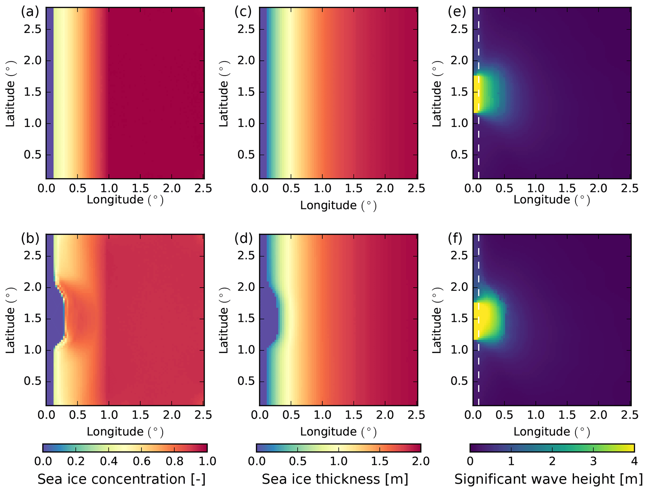
Figure 1Implementation of the WRS in the idealized configuration. (a) and (c) show the initial state of sea ice concentration and thickness (ice-cover average), respectively. (b) and (d) show sea ice concentration and thickness after 72 h in the WW3–LIM3 coupled model. (e) and (f) show the significant wave height Hs distribution after 72 h in the WW3 model and in the WW3–LIM3 coupled model, respectively. The dashed white line in (e) and (f) indicates the position of the ice edge (c=0.15).
2.1 Idealized configuration
In order to test and illustrate the effect of the coupling (Sect. 3), we make use of a simple idealized configuration (see Fig. 1), in which LIM3 is used in a stand-alone mode (without any ocean component). The configuration is a squared domain with 100 by 100 grid cells, with a resolution of 0.03∘ in both directions (corresponding roughly to 3 km). Both models are run on the same grid with the same time step set to 300 s. The coupling time step is also set to 300 s. The sea ice is forced solely by waves, without prescribing any wind or ocean currents. Following Boutin et al. (2018), the simulation starts at rest, with distributions of sea ice concentration (Fig. 1a) and thickness (Fig. 1c) set to represent roughly the conditions that can be found in the MIZ. Starting from the western border, the domain is free of ice over the first ≃ 10 km, after which the ice concentration c increases linearly from 0.4 to 1 about 90 km further eastward (longitude is 0.84∘ E). Ice thickness also increases from west to east following , where Nx is the number of grid cells in the x direction starting from the western border of the ice-covered domain. Waves radiate from part of the western border of the domain, between 1.2 and 1.8∘ latitude, and propagate to the east. The wave spectrum used as forcing at the boundary is extracted at a point south of Svalbard from an Arctic hindcast performed with WW3 described by Stopa et al. (2016). It covers the period of 2 and 3 May 2010, during which a storm occurred in this particular area (Collins et al., 2015). Here we rotate the spectrum so that the direction with the largest density of wave energy is lined up with our x axis. Simulations start on 30 April, at 02:00 GMT, and the attenuation processes (scattering, bottom friction and inelastic flexion dissipation) use the same parameterization as in the reference simulation described by Ardhuin et al. (2018).
2.2 Pan-Arctic configuration
We also make use of the CREG025 configuration (Dupont et al., 2015; Lemieux et al., 2018), which is a regional extraction of the global ORCA025 configuration developed by the Drakkar consortium (Barnier et al., 2006). Although the coupling is solely between LIM3 and WW3, the configuration here also includes the ocean component of NEMO 3.6 (Madec, 2008). CREG025 encompasses the Arctic and parts of the North Atlantic down to 26∘N and has 75 vertical levels and a nominal horizontal resolution of 0.25∘ (≃ 12 km in the Arctic). Both NEMO-LIM3 and WW3 are run on the same grid. Initial conditions for the ocean are taken from the World Ocean Atlas 2009 climatology for temperature and salinity. The initial sea ice thickness and concentration are taken from a long ORCA025 simulation performed by the Drakkar consortium. Along the lateral open boundaries, monthly climatological conditions (comprising sea surface height, 3-D velocities, temperature and salinity) are taken from the same ORCA025 simulation. Regarding the atmospheric forcing, we use the latest version of the Drakkar forcing set (DFS 5.2, which is an updated version of the forcing set described in Brodeau et al., 2010). The choices regarding the parameterization of the wave–ice attenuation are following the ones made in the REF simulation by Ardhuin et al. (2018). The ice flexural strength has however been increased from 0.27 to 0.6 MPa, which is the highest value used in Ardhuin et al. (2018). This choice makes sea ice harder to break and has been made to compensate for the fact that no lateral growth of sea ice is included in our coupled framework.
Three simulations are performed. First we run a simulation based solely on NEMO-LIM3 (referred to as NOT_CPL), covering the period from 1 January 2002 to the end of 2010, in which the already-existing lateral-melt parameterization in LIM3 is activated. The first years of the simulations are allowing for the adjustment of the ocean and sea ice conditions, and we only analyse results from August and September 2010. During that period, the sea ice extent reaches its annual minimum, providing some fetch for the generation of waves, in particular in the Beaufort Sea. The model sea ice extent during the summer of 2010, and more generally the distribution of the sea ice concentration, compares reasonably well with satellite observations (not shown). Note that this period includes a drop in sea ice concentration in the central Arctic, found both in model results and in satellite observations, that has already been documented by Zhao et al. (2018) and attributed to an enhancement of ice divergence in this region in this particular year. This specific period has also been selected as it includes a few storm events, so extreme wave conditions can be investigated. Another simulation (CPL) is initialized from NOT_CPL on 1 August 2010 and run until 9 September 2010. After this date, sea ice extent starts to increase again, and, as our FSD does not allow for the refreezing of sea ice floes, we cannot realistically represent the processes at play during this period.
Finally, we run a simulation over the same period, based solely on WW3 (referred to as WAVE), in which the wave model is forced by sea ice conditions from the NOT_CPL simulation. In order to allow for some spin-up for the waves to develop and break the ice, we exclude the first 3 d from the analysis. In the following, all the results are for the 37 d period between 4 August and 9 September 2010.
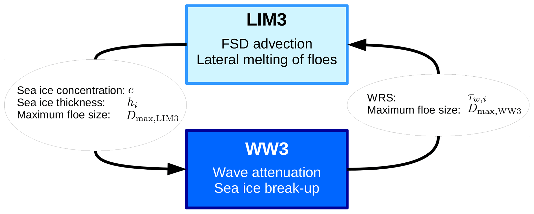
Figure 2Schematic summary of the exchanged information between the sea ice model LIM3 and the wave model WAVEWATCH III® in our coupled framework. The two boxes correspond to the processes accounted for in a given model, while the variables exchanged between the models are listed in the bubbles.
The objective of this section is to present the theoretical background and the practical implementation of the coupling between LIM3 and WW3. Figure 2 shows the principle of the coupling and the variables that are exchanged between the two models. Briefly, LIM3 sends the sea ice thickness, concentration and maximum floe size (estimated from the newly implemented FSD) to WW3. This maximum floe size, referred to as Dmax, represents the largest size of floes remaining after the fragmentation event. These quantities are used by WW3 in order to estimate the wave attenuation and wave-induced sea ice fragmentation. Note that, in general, we refer to sea ice thickness as the cell average of the sea ice thickness distribution gh used as a state variable in LIM3. In the coupling, we actually exchange the ice-cover average sea ice thickness, although this choice does not significantly affect our results. WW3 then returns the WRS to LIM3, as well as the updated maximum floe size if fragmentation has occurred. The occurrence of fragmentation is thus determined in the wave model, depending on the wave conditions (see Boutin et al., 2018). In LIM3, we assume wave-induced fragmentation results in a truncated power law defined for floe sizes up to the maximum floe size estimated in WW3. LIM3 takes into account the WRS in its ice transport equation and advects the sea ice and its FSD, which is defined as an areal distribution. The FSD in LIM3 is also used to estimate lateral melt.
In the following, we describe in more detail the modifications that have been carried out in LIM3 and WW3 in order to couple them and how variables are exchanged between the two models. The coupling allows a new formulation for the sea ice lateral melt in LIM3 (Sect. 3.3).
3.1 Wave radiation stress
Waves transport momentum, and, when they are attenuated by either dissipation or reflection, this momentum is transferred to what has caused this attenuation (Longuet-Higgins, 1977). In the case of sea ice, this momentum loss thus acts as a stress that pushes sea ice in the direction of attenuated waves. Following the study of Williams et al. (2017), in which a WRS was implemented in neXtSIM, the WRS τw,i is computed as
where ρw is the water density; g is gravity; ω, θ and k are, respectively, the radial frequency, direction and wavenumber of waves; and is the source term (negative by convention in WW3) corresponding to wave attenuation by sea ice at a given position.
Once estimated by WW3, the WRS is then sent to the sea ice model and added as an additional term in the momentum equation of LIM3 (Rousset et al., 2015):
in which m is the total mass of ice and snow per unit of area; u is the ice velocity vector; σ is the internal stress tensor; f is the Coriolis parameter; k is a unit vector pointing upwards; η is the sea surface elevation; c is the sea ice concentration; and τa and τo are the atmospheric and oceanic stresses, respectively. In contrast to τa and τo, τw,i does not need to be multiplied by c, as the wave attenuation estimation in WW3 (and hence the WRS) is already scaled by the sea ice concentration to account for the partial sea ice cover.
Figure 1 illustrates the effect of the implementation of the WRS in our simple model. Here, the sea ice thermodynamics are switched off so that we only simulate the effect of waves pushing sea ice. Under the action of waves, the sea ice edge shifts eastward, resulting in an increase in the sea ice concentration (panel b). As the sea ice near the sea ice edge is compacted, it creates a sharp gradient in sea ice concentration and thickness (panels b, d). When comparing panels (e) and (f), it is clear that wave attenuation also responds to this change in the sea ice properties: waves tend to penetrate further eastward when the sea ice edge retreats to the east but are then attenuated faster in the compacted sea ice.
3.2 Floe size distribution and sea ice fragmentation
As mentioned earlier, waves can break sea ice and thus impact the sea ice floe size. It is therefore necessary to exchange parameters defining the FSD between the two models. An FSD has been previously implemented in WW3 by Boutin et al. (2018) and is used to estimate the wave attenuation due to inelastic flexure and scattering. Following the work by Toyota et al. (2011) and Dumont et al. (2011), we assume that the FSD in WW3 follows a truncated power law between a minimum floe size, Dmin, and a maximum floe size, Dmax. Dmin corresponds to the minimum floe size that can be generated by waves and is of the order of O(10 m), while Dmax depends on the local wave properties and is used to estimate the level of sea ice fragmentation. As Dmin is assumed to be constant in WW3, the FSD in the wave model is thus only a function of Dmax. Ideally, WW3 would therefore send the value of Dmax to the sea ice model, where it would be advected and updated due to the effects of thermodynamical and mechanical processes and then sent back to WW3. Yet, Dmax is not an area-conserved quantity and therefore cannot be advected as a tracer (Williams et al., 2017). Instead, we thus choose to define an FSD in LIM3, from which a maximum floe size can be estimated and then sent to the wave model.
There is no FSD included in the standard version of LIM3. However, recent work by Zhang et al. (2015) and Horvat and Tziperman (2015) has proposed ways to implement an FSD in sea ice models, following what is done for the sea ice thickness distribution (which is a state variable of any multi-category sea ice model). In their study, Horvat and Tziperman (2015) use a joint thickness and floe size distribution in order to represent the evolution of sea ice floes affected by a great variety of processes not necessarily related to waves (e.g. welding, refreezing, ridging). The approach by Zhang et al. (2015) is simpler and computationally cheaper, as it assumes that all floes of a given size have the same ice thickness distribution, allowing the FSD to be treated independently of the sea ice thickness distribution. To do so, they hypothesize that the FSD mostly results from the fragmentation of large unbroken floes randomly yielding floes of any size smaller than the original ones. In this study, we choose to follow the simpler approach of Zhang et al. (2015), as we only consider the effects of wave-induced sea ice fragmentation and lateral melt on the FSD evolution, and our formulation of lateral melt does not depend on sea ice thickness (see Sect. 3.3). Therefore, we can consider the distribution of sea ice thickness and floes independently, defined, respectively, as
and
h being the sea ice thickness and D being the caliper diameter of the floes as defined by Rothrock and Thorndike (1984). In these definitions, A is the total area considered, and ah and aD are the areas within A covered by sea ice with thickness between h and h+dh and floes with diameters between D and D+dD, respectively. The evolution of the FSD depends on sea ice advection, thermodynamics and mechanical processes and is given by
in which u corresponds to the sea ice velocity vector; Φth is a redistribution function of floe size due to thermodynamic processes (i.e. lateral growth and melt); and Φm is a mechanical redistribution function associated with processes like fragmentation, lead opening, ridging and rafting. In our implementation, the only processes affecting the FSD are lateral melt and sea ice fragmentation. Other processes driving the evolution of the sea ice concentration do not modify the shape of the FSD. From a technical point of view, the FSD in LIM3 is implemented as an areal distribution divided into floe size categories. It is advected in the same way as other sea ice tracers like sea ice concentration or thickness.
In their sea ice model neXtSIM, Williams et al. (2017) have also implemented an FSD but in a different way than Zhang et al. (2015). Indeed, they assume that the FSD follows a truncated power law between a minimum and maximum floe size, similar to the assumption made in WW3. Thus, in their model, the FSD always obeys a power law with a constant exponent and only evolves when sea ice fragmentation results in a reduction of the maximum floe size. Here we combine the approaches of Zhang et al. (2015) and Williams et al. (2017) and implement an FSD in LIM3 that evolves following Eq. (7) but that also undergoes a redistribution after each fragmentation event that makes it tend towards the power law assumed in WW3. Thus, in contrast to Williams et al. (2017), we do not make any assumption about the shape of the FSD in general, but, just as they do, we assume that after being fragmented by waves, the FSD follows a power law with a maximum floe size that depends on the local sea state. Our implementation only differs from the one carried out by Zhang et al. (2015) in the way we have implemented the redistribution: instead of assuming that the broken sea ice is redistributed uniformly among the smaller floes after each fragmentation event (that actually quickly tends towards a power-law distribution with a varying exponent depending on the wave state in their study), we assume that wave-induced fragmentation results in a truncated power law with a constant exponent defined for floe sizes up to the value of Dmax received from WW3, under the constraint of conservation of area. As a result, the FSD resulting from fragmentation in LIM3 is the same as the one assumed in WW3, ensuring coherence between the two models. The exponent of the truncated power law corresponds to a value of about −1.85 for the cumulative-number-of-floes distribution, which is the distribution generally used to represent the FSD in the scientific literature (e.g. Toyota et al., 2011; Herman et al., 2018). This value originates from the parameterization of wave-induced fragmentation by Dumont et al. (2011) and is the one used in WW3 by Boutin et al. (2018). This redistribution is instantaneous in LIM3, which we justify by the fact that fragmentation is a violent process that can completely change an FSD on timescales of a few minutes to a few hours (see Collins et al., 2015, for a description of such an event). Note that the redistribution of the FSD due to fragmentation transfers sea ice from large floes to smaller floes. Combined with lateral melt, a process that also reduces the floe size, the action of waves in our model always reduces the floe size. The details of the mechanical redistribution function Φm are mostly following what has been proposed by Zhang et al. (2015) and are given in Appendix A.
Now that both models include an FSD, the two models can be coupled in order to represent the effect of the wave-induced sea ice fragmentation, the occurrence of which in LIM3 is determined depending on information provided by WW3. As mentioned earlier, sea ice fragmentation in WW3 is determined by local wave properties, and fragmentation events result in an update of the maximum floe size Dmax which controls the FSD. It is thus logical to define a similar parameter Dmax,LIM3 from the FSD of LIM3 that ideally equals the value of Dmax in WW3. However, estimating Dmax,LIM3 is not straightforward. Indeed, our FSD implementation requires not only that Dmax,LIM3 corresponds to the upper limit of the power law followed by the FSD in both WW3 and LIM3 but also that Dmax,LIM3 can evolve with the deviations of the FSD in LIM3 from this power law under the effects of sea ice advection and thermodynamics. Calling the distribution corresponding to an FSD following the assumed power law, we thus define Dmax,LIM3 as the greatest value of D for which the following condition applies:
in which is an ad hoc parameter allowing the value of Dmax,LIM3 to remain unchanged when the FSD slightly deviates from the assumed power law (after lateral melt or advection for instance). Setting to equal 1 results in an immediate reduction of Dmax if there is a negligible reduction in the proportion of large floes in the FSD after a fragmentation event (when lateral melt occurs for instance). This can be problematic, as reducing the value of Dmax during a fragmentation event allows for the wave to propagate further, generating more fragmentation. Values of between 0.5 and 0.8 allow for little variation in the FSD while keeping the same value of Dmax, thus giving more weight to fragmentation than to other processes in the estimation of Dmax. Overall the choice of in this range does not significantly affect our results. In the following, is set to 0.5.
Floes that have never been broken by waves have no physical reason to follow this truncated power law. In practice, if we consider a discrete number N of floe size categories, the Nth category should represent these unbroken floes, with a different condition to set the value of Dmax,LIM3 to DN (the upper size limit of this category). We thus consider sea ice in a grid cell as unbroken only if most of its floes belong to this Nth category, so only if gN>0.5c, gN being the value of the FSD function associated with the Nth category and c being the total sea ice concentration.
In all of our simulations, sea ice is initialized as unbroken everywhere so that gN=c, and . As soon as wave-induced fragmentation occurs, Dmax,LIM3 is updated. To do so, the received value of Dmax is rounded up to the upper limit of the category it lies in. Dmax,LIM3 is therefore slightly greater than the value received from WW3, with an error that depends on the width of its associated floe size category.
Tests with the simplified domain were also performed with different numbers and widths of floe categories to investigate the sensitivity of the results to those parameters. This sensitivity remains very small as long as the widths of the categories are smaller than 10 m and the categories cover a range of floe sizes larger than 300 m. In the following, we use N=60 floe size categories that we define as follows:
-
A first category corresponds to the sea ice floes that are already broken but cannot be broken anymore (D0=8 m, D1=13 m). D0 represents the smallest floe size possible in the model and is set to 8 m in order to agree with the minimum floe size used in LIM3 to estimate lateral melt from the formula by Lüpkes et al. (2012). D0 is also on the same order as the size of the smallest floes that can be generated by wave-induced fragmentation (Mellor, 1986) and therefore is an acceptable value for the lower limit Dmin that the truncated power law is assumed to follow after wave-induced fragmentation.
-
There are 58 categories for which m, with .
-
A last category represents unbroken floes ( m, DN=1000 m). This value of DN=1000 m is set as it is 1 order of magnitude higher than the floe size generated by waves (Toyota et al., 2011).
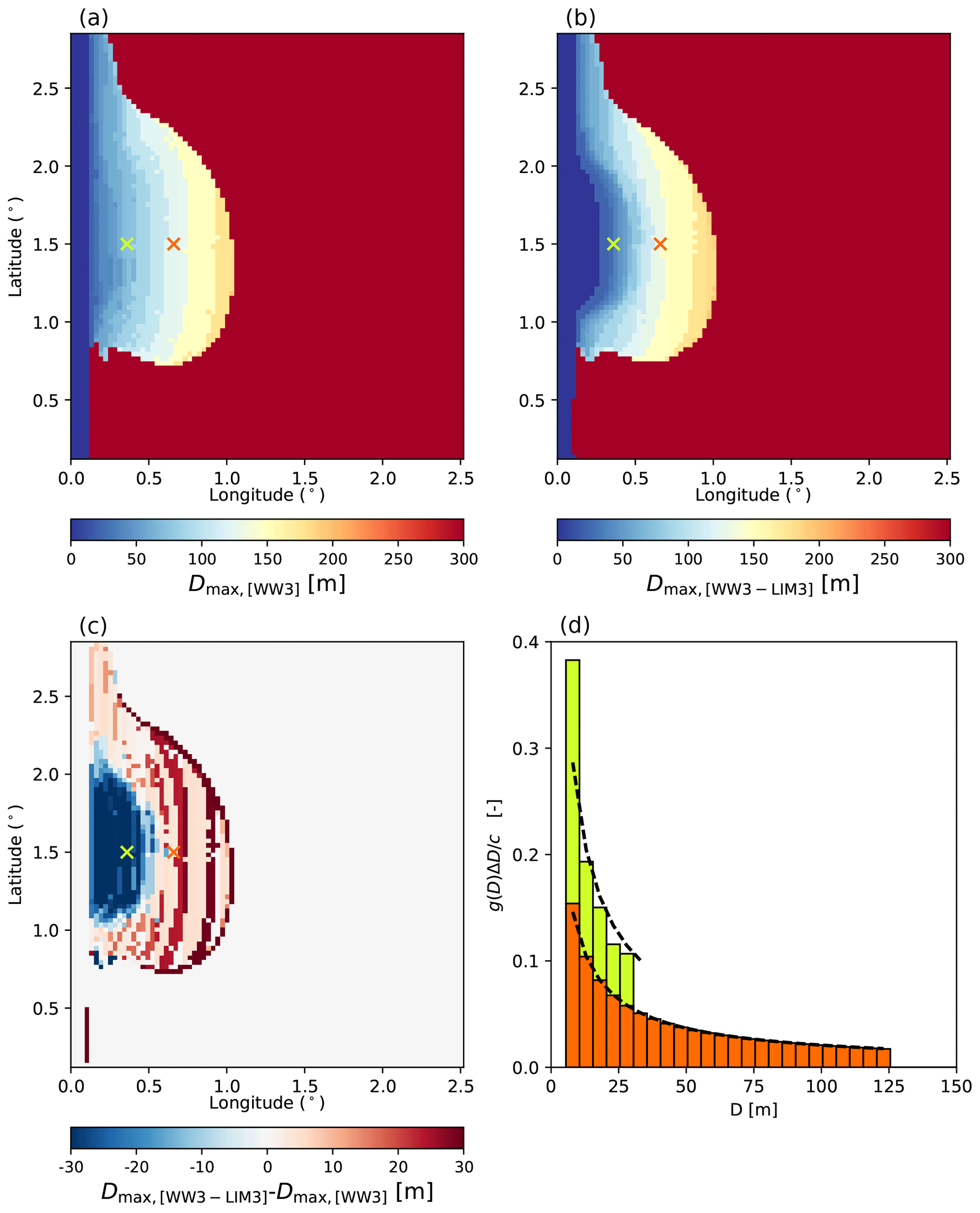
Figure 3Snapshots of Dmax from the uncoupled WW3 (a) and the WW3–LIM3 (b) simulations after 72 h and the difference between the two (c). Panel (d) shows the FSD from the WW3–LIM3 run at two locations indicated with crosses on (a–c). The dashed black line in (d) corresponds to the theoretical power-law FSD assumed in WW3.
We evaluate the effect of this part of the coupling between WW3 and LIM3, as well as the robustness of the implementation of the FSD in LIM3, by looking at the same two simulations in our idealized configuration as presented in Fig. 1 and comparing an uncoupled WW3 simulation with a coupled WW3–LIM3 simulation (Fig. 3). Sea ice thermodynamics are switched off in the WW3–LIM3 simulation. In the uncoupled WW3 simulation, Dmax evolves depending on the sea state, but sea ice thickness and concentration are constant. In the WW3–LIM3 coupled simulation, sea ice properties are all evolving as sea ice is pushed by the WRS, and the FSD is advected in LIM3. The comparison between Dmax estimated from the WW3 simulation and Dmax,LIM3 from the coupled simulation is shown in Fig. 3a–c. The pattern of broken sea ice is broadly similar in the two simulations (Fig. 3a, b), despite the sea ice retreat due to the WRS in the coupled case. Differences in Dmax (Fig. 3c) follow the wave height differences already commented on in Fig. 1e and f. Indeed, the retreat of the ice edge due to the WRS allows for waves to propagate further with less attenuation, thus involving more sea ice fragmentation and a lower maximum floe size close to the open ocean in the coupled simulation. Further east in the MIZ, the sea ice compacted by the WRS effect generates stronger wave attenuation and thus less sea ice fragmentation and a larger maximum floe size when compared to the uncoupled simulation. Both effects partly compensate for each other, so the shift in the ice edge position has little effect on the spatial extent of broken ice. Figure 3d shows the FSD at two locations in the domain. At both locations, the distribution of ice-covered area within the different categories agrees very well between LIM3 and the truncated power law assumed in WW3. The area covered by floes of the smallest possible size in LIM3 is nevertheless greater than it would be if the FSD was exactly following the truncated power law. This is because floes that have been broken down into the smallest possible size do not contribute to the redistribution (see Appendix A) and accumulate in this category since no lateral growth occurs. Note that a coupled simulation in which advection had been deactivated was also run to ensure that, in a case with unaffected initial sea ice properties, no significant discrepancies were noticeable for both significant wave height and maximum floe size between a coupled and an uncoupled simulation (not shown).
3.3 Lateral melt
A parameterization to account for the sea ice lateral melt is already implemented in LIM3. Its formulation follows Steele (1992):
where c is the sea ice concentration; wlat is the lateral-melt rate, which depends on the difference between sea ice and sea surface temperatures taken from Maykut and Perovich (1987); and α is a coefficient which varies with the floe geometry. By default, α=0.66, which is the average value of the non-circularity of floes obtained by Rothrock and Thorndike (1984). By default, 〈D〉, which represents the average floe size, is a function of the sea ice concentration obtained empirically from observational data by Lüpkes et al. (2012):
where β=1 and c* is introduced to avoid a singularity at c=1 and is defined as
This relationship finds a value of 〈D〉 that increases very little from its minimum value (set to D0) as long as the sea ice concentration remains lower than ≃ 0.6 (see Fig. 3 from Lüpkes et al., 2012). In the following, we refer to this lateral-melt parameterization as the parameterization of Lüpkes et al. (2012), although we acknowledge that the work of Lüpkes et al. (2012) only provides a relationship between the average floe size and the sea ice concentration.
In the case of our coupled model, we estimate an FSD, and thus it makes sense to implement a parameterization of the lateral melt that depends explicitly on the FSD rather than on sea ice concentration. Following the work by Horvat and Tziperman (2015) and Roach et al. (2018b), we estimate the lateral melt as
where Φth is the change in the FSD due to lateral melt (see Eq. 7). Note that lateral melt for floes in the unbroken category is computed assuming that all the floes have a size D of 1000 m. Note also that Horvat and Tziperman (2015) and Roach et al. (2018b) represent the evolution of the floe radius and therefore include in their equation a term they call Gr, representing , the rate at which the floe radius changes due to lateral growth or melt. In our case, we represent the evolution of the floe diameter, and the rate at which it changes due to lateral growth or melt is thus equal to (hence the addition of a factor of 2 in Eq. 12).
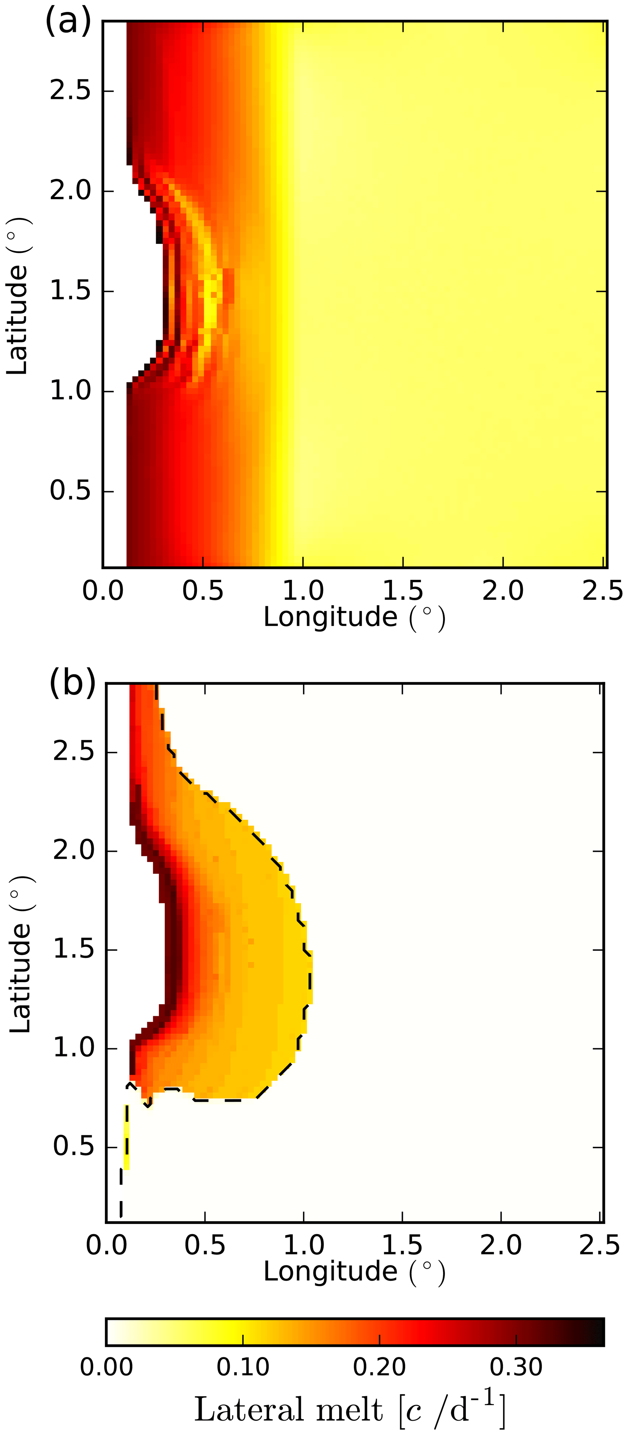
Figure 4Lateral-melt rates (estimated as percentage of sea ice concentration lost per day) estimated by the coupled model after 72 h of simulation using the parameterization of Lüpkes et al. (2012) (a) or the parameterization developed in this study accounting for wave-induced sea ice fragmentation (b). The dashed black contour in panel (b) indicates m and thus represents the limit between broken and unbroken sea ice.
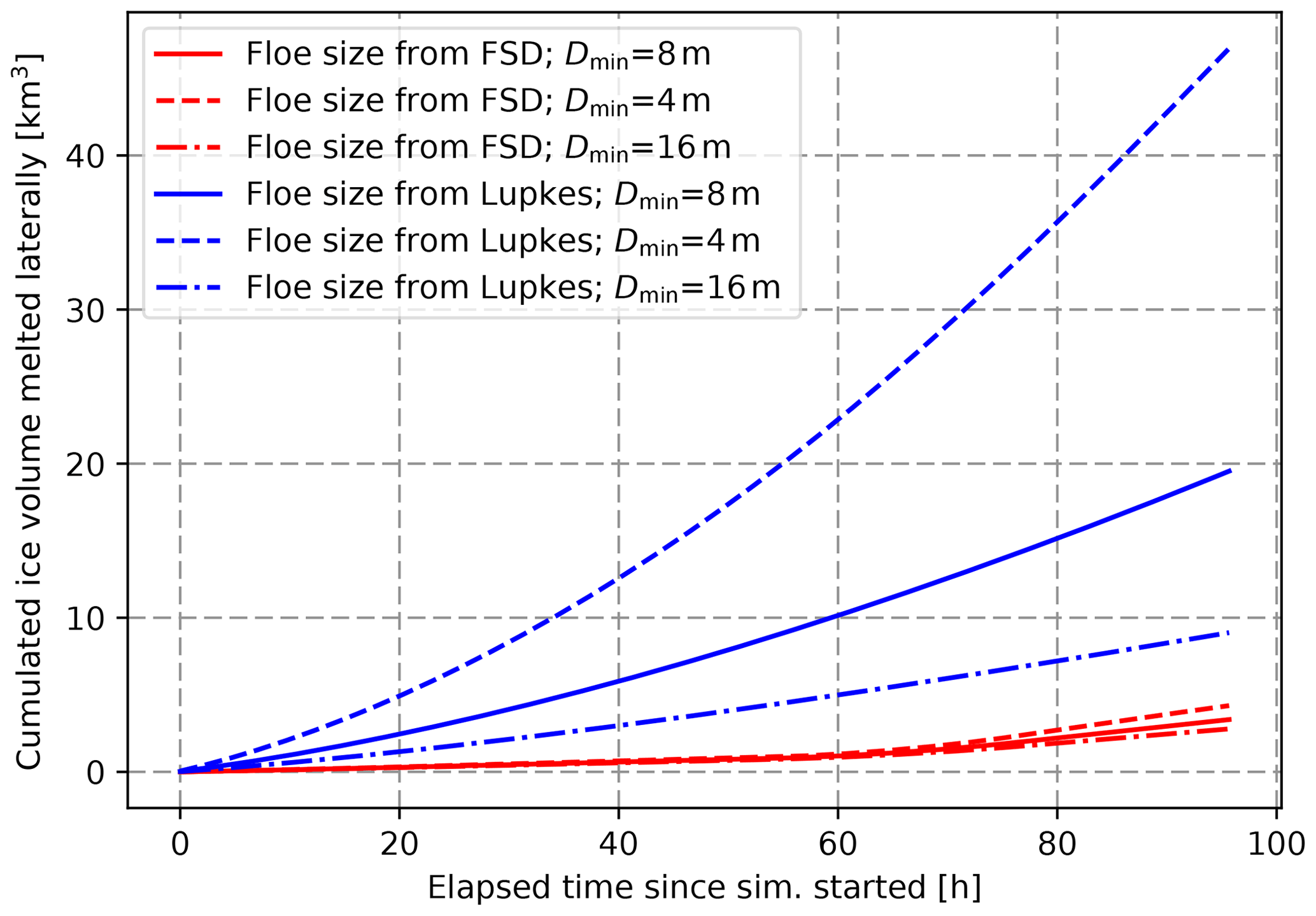
Figure 5Temporal evolution of the sea ice volume loss due to lateral melt integrated over the whole domain for simulations similar to the one presented in Fig. 4 but for different values of Dmin. The two colours correspond to the two lateral-melt parameterizations used in this study.
We run two simulations in which the lateral melt is estimated either from the formulation of Lüpkes et al. (2012) or by our new formulation, which accounts for the FSD that is determined by both the sea ice and the wave models (Fig. 4). Here we only activate the lateral melt and turn off the basal and surface melt. The sea surface temperature is set constant to T=0.3 ∘C. Floe size categories are the same as in Sect. 3.2. In the case of the Lüpkes et al. (2012) parameterization (Fig. 4a), lateral melt only depends on the sea ice concentration and thus follows its distribution. In the second case (Fig. 4b), lateral melt is highly constrained by both the distribution of the sea state and ice properties and is only significant where the sea ice is broken. Melt rates are overall higher when estimated from the Lüpkes et al. (2012) parameterization, mostly due to the fact that the average floe size in the uncoupled run is very close to D0 for a wide range of concentrations. Unlike the parameterization that we propose here, the parameterization of Lüpkes et al. (2012) results in a significant lateral melt far from the ice edge, where sea ice is mostly compact and unbroken, which is likely unphysical.
We find that the results are also sensitive to the choice of Dmin, regardless of the parameterization used. In the case of our FSD, the sensitivity arises from the use of Dmin to compute the average diameter of the smallest floe size category, which is the category most affected by lateral melt. In order to quantify the sensitivity to the choice of Dmin, we run similar experiments to the one presented in Fig. 4, varying this time the value of Dmin (Fig. 5). When using the parameterization of Lüpkes et al. (2012) (Eqs. 10 and 11), the volume of sea ice melted laterally roughly doubles when Dmin is divided by 2 compared to the reference simulation (using Dmin=8 m). In the case of our FSD, the sensitivity is still large but greatly reduced, with an increase of only 20 % in response to the same change in Dmin. Figure 5 also illustrates the strong differences in melted volume between the two parameterizations, with much less lateral melt when computed using the FSD developed here.
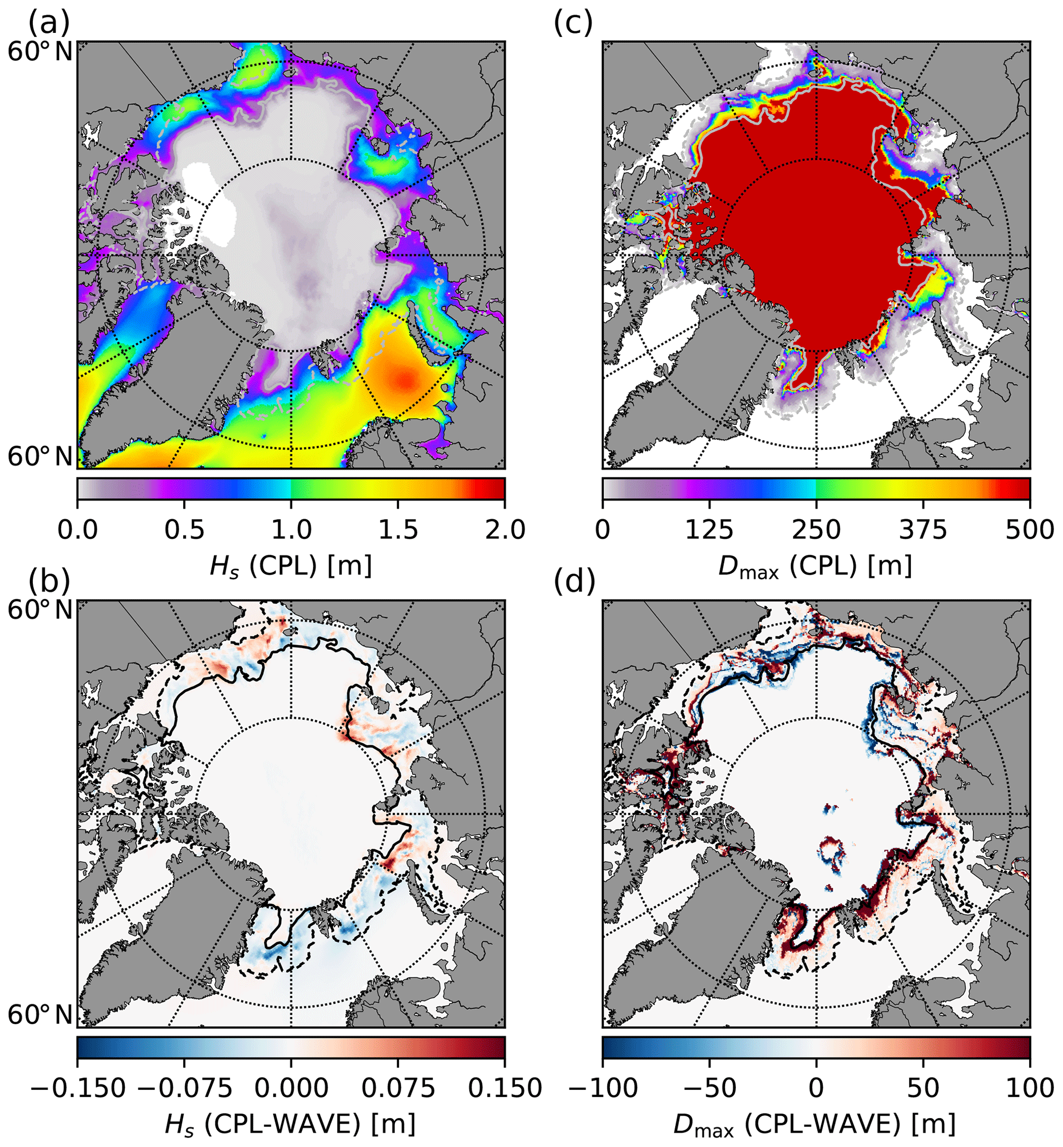
Figure 6Significant wave height (a) and maximum floe size (c) in the CPL simulation averaged over the period 3 August to 9 September 2010 and the differences with the WAVE simulations (b, d). The black and grey contours delimit the MIZ in the CPL simulation, defined here as m. Note that the sea ice conditions from the NOT_CPL run are used as forcing for the WAVE run and are thus similar in the WAVE and the NOT_CPL runs.
In this section we compare the three simulations performed with the CREG025 configuration described in Sect. 2.2 in order to quantify the impact of the coupling on wave, sea ice and ocean surface properties. To evaluate the impact of waves in the MIZ, we first need to define the MIZ in our model. Various criteria, relying on sea ice concentration, floe size or the region where waves impact the sea ice floe size, have been previously used to delimit the MIZ (see for instance Dumont et al., 2011; Strong and Rigor, 2013; Sutherland and Dumont, 2018). Here we take the following definition based on the maximum floe size: m, where 〈Dmax〉 is the average of the maximum floe size over the study period. Physically, it roughly corresponds to the region where sea ice has been broken during a time period that is long enough for the average maximum floe size to become smaller than 1000 m (which is the limit between the broken and unbroken ice). Note that our results are not dependent on the definition of the MIZ.
4.1 Effect of the coupling at the pan-Arctic scale
4.1.1 Impact on the wave properties
First, we examine the differences between the CPL and WAVE simulations, corresponding, respectively, to the coupled WW3–LIM3 run and a run performed with WW3 in stand-alone mode forced with sea ice properties from NOT_CPL. When looking at the differences in significant wave height Hs (Fig. 6b), we find that they are small, not exceeding ≃ 15 cm on average. Moreover, the two runs exhibit similar patterns of Dmax, indicating that the wave-induced fragmentation is similar in the two simulations (Fig. 6d). Locally, in the Barents and Greenland seas for instance, the differences in Dmax can be significant, due to the specific ice drift conditions in these regions. Indeed, the overall southward drift of sea ice tends to bring unbroken sea ice from the central Arctic to regions where sea ice is broken up, increasing Dmax in the CPL simulation. The signs of the differences in Hs and Dmax vary regionally. This might be due to the differences in sea ice concentration and thickness as the wave attenuation in sea ice is very sensitive to sea ice properties (see for instance Ardhuin et al., 2018). Certainly, the pattern of the differences in Hs between the CPL and WAVE runs is consistent with the differences in sea ice concentration and thickness between the CPL and the NOT_CPL simulations (Fig. 7), with higher waves found in regions where ice is less concentrated and thinner.
4.1.2 Impact on the sea ice and sea surface properties
We now focus on the effect of adding a wave component on the sea ice properties by comparing results from the CPL and NOT_CPL simulations. Figure 7 shows the pan-Arctic distribution of the sea ice thickness and concentration averaged over the 37 d considered in the CPL simulation, as well as the differences with the NOT_CPL simulation. These differences are concentrated in the vicinity of the ice edge and exhibit different signs depending on the location. Positive and negative anomalies tend to compensate for each other, resulting in weak overall differences in sea ice extent and volume when averaging over the full Arctic Basin. If we only consider the MIZ, the sea ice volume and area decrease by about 3 % and 2 %, respectively, between CPL and NOT_CPL (Fig. 8b). Locally, however, these variations can be much larger. In the MIZ of the Beaufort Sea for instance, the relative changes can be as high as 10 % for grid-cell-average thickness.
There are also differences in sea surface properties between the two simulations (Fig. 9), with average increases in sea surface temperature (SST) and salinity (SSS) in the MIZ as high as 0.5 ∘C and 0.8 psu locally, respectively. It is worth noting that, in contrast to the sea ice properties, the sign of the differences in SST and SSS tends to be positive, i.e. warmer and saltier in the CPL experiment compared to the NOT_CPL one.

Figure 7Sea ice concentration and thickness in the CPL simulation (a, c) and the differences with NOT_CPL (b, d) averaged over the period 4 August 2010 to 9 September 2010. The black contours delimit the MIZ in the CPL simulation, defined here as m.
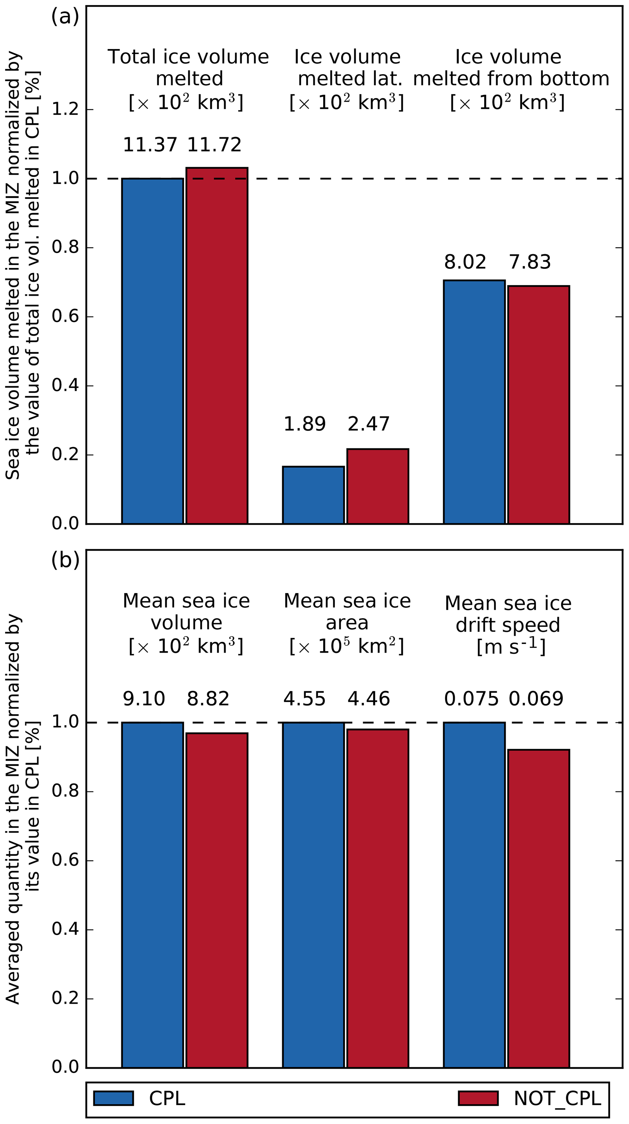
Figure 8(a) Sea ice volume melted (in 102 km3) integrated over the MIZ and over the period between 4 August and 9 September 2010 in the CPL and the NOT_CPL simulations. Here the MIZ is defined as the region where m in the CPL run. The contributions from lateral melt and bottom melt to the total melt for both simulations are also represented. (b) Mean sea ice volume (in 102 km3), area (in 105 km2) and drift speed (in m s−1) in the MIZ over the same period. Values for each simulation are found above their associated bar.
4.1.3 Thermodynamical effect of the coupling
Given that there is no coupling between the ocean and the wave components, the difference in sea surface properties must arise from variations in sea ice conditions and in particular the sea ice melt, and we now investigate this further. Figure 10a and b show the total sea ice volume loss from lateral melt during the study period in the CPL run as well as the difference between this and the same quantity from the NOT_CPL run. The sea ice volume melted by lateral melt shows very similar spatial patterns in the two simulations, although it is estimated from two very different parameterizations (Eqs. 9 and 12) and although lateral melt estimated by the parameterization from Lüpkes et al. (2012) tends to be lower in CPL. The difference is substantial, the sea ice volume melted in the MIZ in CPL being 30 % lower than in NOT_CPL (Fig. 8a). Another signal is found in the central Arctic, while no lateral melt occurs in this region in CPL. This signal actually arises from the combination of the drop in sea ice concentration that happens in the region in August 2010 (Zhao et al., 2018) and the use of the parameterization by Lüpkes et al. (2012) to estimate floe size and resulting lateral melt in NOT_CPL. Indeed, lower sea ice concentration values correspond to estimated average floe sizes below 100 m when estimated from the parameterization by Lüpkes et al. (2012), and thus some lateral melt is triggered. In contrast, the absence of waves in the middle of the sea ice pack in CPL leaves sea ice unbroken in this region, preventing lateral melt from occurring. An average floe size of ≃ 100 m in the middle of the pack seems somewhat unrealistic and highlights the limitations of estimating the floe size using the Lüpkes et al. (2012) parameterization in pan-Arctic configurations. Absence of lateral melt in the central Arctic in CPL explains the excess in sea ice concentration when compared to the uncoupled simulation (Fig. 7b). Moreover, the fact that differences in lateral melt between the two simulations are mostly negative means that it cannot explain the regional patterns found in the distribution of sea ice property differences.
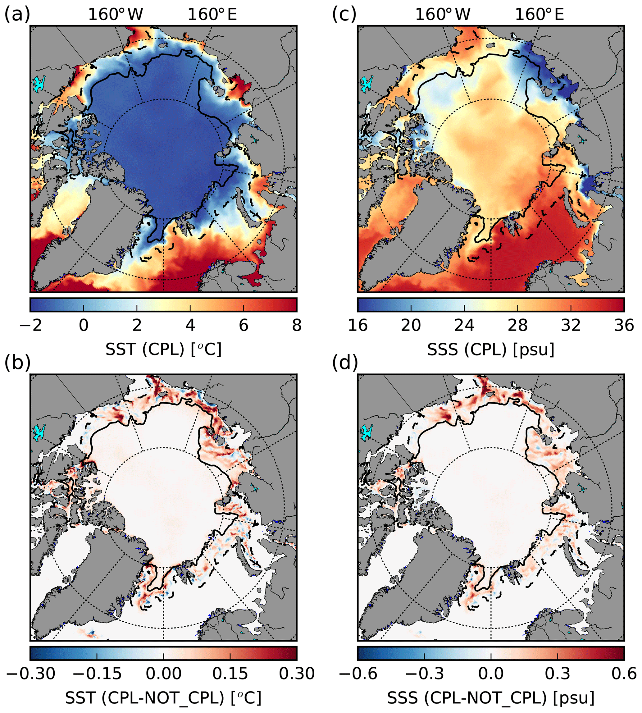
Figure 9SST (a) and SSS (c) in the CPL run for the period between 4 August and 9 September 2010 and the difference with NOT_CPL (b, d). The black contours delimit the MIZ in the CPL simulation, defined here as m.
Figure 10c and d show the differences in bottom and total ice melt between the CPL and NOT_CPL simulations. The spatial distributions of the differences in bottom and total ice melt are very similar, meaning that the variations in bottom melt dominate the differences in sea ice melt between CPL and NOT_CPL, although the bottom melt is computed the same way in the two simulations. This result is confirmed by rerunning a coupled and an uncoupled simulation of NEMO-LIM3 while deactivating lateral melt (not shown), which yields differences in total melt distribution almost identical to the ones presented in Fig. 10c and d.
The total melted sea ice volume, once integrated over the MIZ, increases by 3 % between CPL and NOT_CPL, mainly due to the larger volume of sea ice melted laterally in NOT_CPL (Fig. 8a). In parallel, bottom melt slightly decreases by ≃ 1 % between these two simulations. This result masks the fact that the regional differences of total melt are dominated by bottom melt. An explanation is that bottom and lateral melt both depend on the available heat in the surface layer, either directly for bottom melt or indirectly through lateral melt that depends on the SST. If lateral melt occurs, it removes heat from the surface layer, therefore reducing the bottom melt capacity. Conversely, if this heat is not used for lateral melt, it remains available for bottom melt. The overall decrease in bottom melt in the MIZ between CPL and NOT_CPL visible in Fig. 8a therefore mostly results from the compensation for the increase in lateral melt due to the change in parameterization, as can be seen in Fig. 10b and c. This compensation mechanism has been reported before by Tsamados et al. (2015) and Roach et al. (2018a) and also by Roach et al. (2018b) and Bateson et al. (2019), who compare two runs of the sea ice model CICE, one with the standard lateral-melt parameterization using a constant floe size of 300 m and one using an FSD (allowing floes smaller than 300 m). In our case, this compensation is strong enough, and completely deactivating lateral melt in both runs has a negligible effect on the quantity of melted ice in our simulations.
4.1.4 Dynamical effect of the coupling
The differences in lateral melt between the CPL and the NOT_CPL runs cannot explain the differences in sea ice and sea surface properties seen in Figs. 7 and 9. We thus investigate the impact of the WRS on the sea ice conditions and melt. Figure 10e and f show the mean directions of the wind stress and the WRS in the CPL simulation and the ratio of WRS magnitude to wind stress, respectively. This ratio is generally low, not exceeding 15% of the wind stress in the eastern Barents Sea, where the WRS reaches its highest magnitude. This is much smaller than the values retrieved from satellite observations in the Southern Ocean, where the wind stress and the WRS can be of comparable magnitude (Stopa et al., 2018a). It is also worth noting that the regions where this relative importance of the WRS compared to the wind is large do not always coincide with regions where differences in sea ice properties are significant (Fig. 7). In the Beaufort Sea for instance, there is substantially less sea ice melt in the CPL simulation than in the NOT_CPL one, although the ratios of WRS over the wind stress are only on the order of a few percent (Fig. 10f). The opposite situation is visible in the Barents Sea, where the high relative influence of the WRS does not result in a significant increase in the sea ice melt when the effect of the waves is included. Therefore, there is no direct relationship between the intensity of the WRS and the differences in sea ice and sea surface properties between the coupled and uncoupled simulations. In the Southern Ocean, Stopa et al. (2018a) found that the orientation of the WRS, which tends to be orthogonal to the sea ice edge, might explain why WRS is as important as the wind (that tends to vary in direction much more over time) in determining the position of the sea ice edge. Similarly, here, we found that the WRS is very often orientated orthogonally to the ice edge, towards packed ice. This is due to the fact that the longer waves encounter sea ice on their path, the more they are attenuated. The direction of propagating waves at a given point in sea ice is then generally imposed by the waves that have travelled the shortest distance in sea ice. This is particularly visible in some parts of the Greenland and Kara seas, where wind and wave stresses have opposite directions on average. In the Chukchi and the eastern Beaufort seas, the WRS is orthogonal to the wind stress. In contrast, in the Laptev Sea, the directions of the WRS and the wind stress roughly align and thus work together in setting the position of the sea ice edge in the CPL run. However, at the pan-Arctic scale, there is no clear relationship between the WRS direction and the differences in sea ice melt induced by the WRS in the CPL simulation.
The primary effect of the WRS is to push sea ice, modifying the intensity and the direction of the sea ice drift. This impact is significant in the MIZ, where the average sea ice drift velocity increases by ≃ 9 % between the CPL and the NOT_CPL runs (Fig. 8b). This overall increase in the sea ice velocity can be explained by the fact that both WRS and sea ice drift have a dependency on wind direction. As was the case for sea ice thickness and concentration, the distribution of the differences in sea ice drift velocity between the two simulations varies strongly depending on the region considered (not shown) but exhibits no clear relationship at the pan-Arctic scale that could explain the differences in sea ice melt induced by the WRS.
In the following we investigate in further detail the wave–sea ice interactions in two regions during storms. Indeed, although the differences between the CPL and NOT_CPL run at the pan-Arctic scale remain small, it is clear that the way the waves can influence the sea ice and the ocean surface would depend on the local properties of the waves, wind, sea ice and ocean surface.
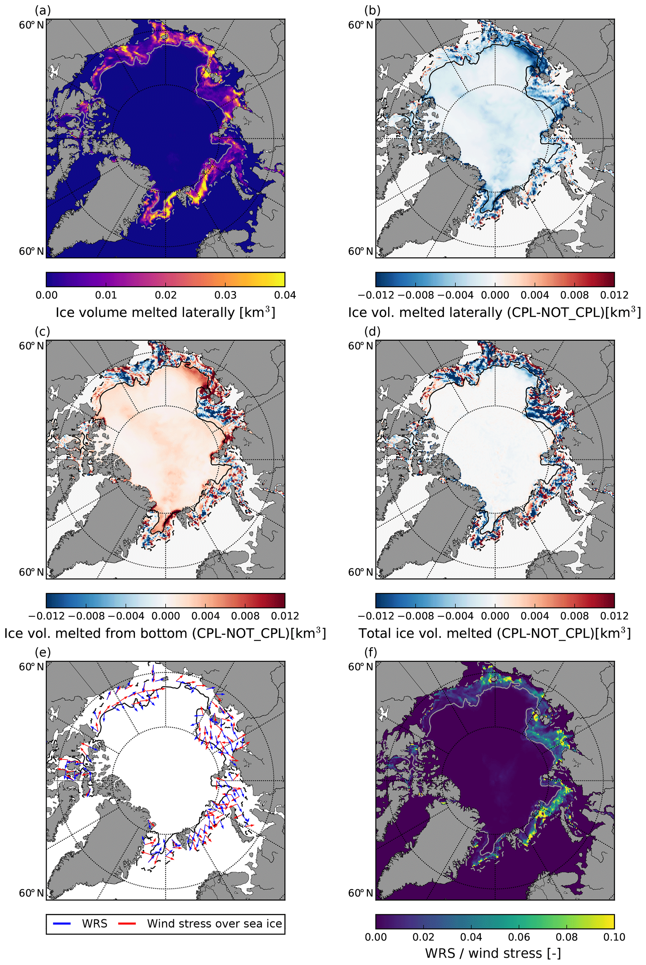
Figure 10Volume of sea ice melted by lateral melt in the CPL simulation over the period between 4 August and 9 September 2010 (a). Differences between the CPL and the NOT_CPL runs of lateral melt (b), bottom melt (c) and total melt (d). (e) Wind stress (red) and WRS (blue) averaged over the same period between 4 August and 9 September 2010 in the CPL simulation. Note that the WRS has been multiplied by a factor of 10 in order to improve readability. (f) Distribution of the relative magnitude of WRS over the wind stress. The grey contours represent the position of the ice edge (c=0.15) on the first day (solid line) and last day (dashed line) of the period considered in the CPL simulation.
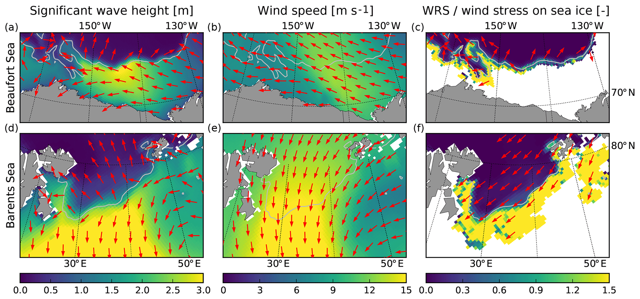
Figure 11Significant wave height and wave mean direction of propagation (a, d), wind speed (b, e) and WRS (c, f) simulated by the CPL run during the storms that occurred in the Beaufort Sea (a–c) and in the Barents Sea (d–f) on 16–17 August 2010. The grey contours indicate the position of the sea ice edge determined from the averaged sea ice concentration (c=0.15).
4.2 Regional impacts of wave–sea ice interactions during storm events
4.2.1 Case 1 – storm in the Beaufort Sea (16–17 August 2010)
We first focus on a storm event that occurred near the MIZ in the Beaufort Sea on 16–17 August 2010 (Figs. 11a–c and 12a, e). During the storm, waves and winds are oriented towards the north-west on the west side of the domain but towards the west on the east side. Wave height and wind speed reach up to 3 and 12 m s−1 (Fig. 11a, b), respectively, while they do not exceed 1 and 7 m s−1, respectively, during the 3 d preceding the storm (not shown). Before the event, the south Beaufort Sea is ice-free, and the position of the sea ice edge (defined at the 15 % sea ice concentration contour) is highly irregular, with the presence of an ice tongue centred around 72∘ N and 155∘ W that is exposed upwind on its eastern side but downwind on its western side during the storm. This sea ice tongue is composed of relatively thick ice (≥ 1 m). During the storm, sea ice breaks all over the ice tongue in the western part of the domain but not further than ≃ 40 km after the sea ice edge. Both the waves and the wind stresses push the ice to the west (Fig. 11b, c), accelerating the drift that is directed north-west (Fig. 12a, c), as was already the case before the storm (not shown). The wave action is particularly effective at the location of the sea ice tongue, where the WRS has an amplitude comparable to the wind stress over sea ice (Fig. 11c). As a consequence, the sea ice drift is substantially accelerated (Fig. 12c). The effect of the waves results in large changes in the sea ice thickness pattern (when comparing the CPL and NOT_CPL runs), with a decrease on the eastern part of the tongue but an increase on the western part (Fig. 12g). Outside of the sea ice tongue, the differences between the simulations are very small, likely because of the sharp sea ice thickness gradient opposing internal resistance to deformation (Fig. 12e) and the relatively small effect of the WRS compared to the wind stress (Fig. 11c).
The differences in sea ice properties around the sea ice tongue between the two runs also result in changes in SST and SSS, with increases of around 1 ∘C and 1 psu, respectively, on the eastern side of the sea ice tongue and a decrease of roughly the same magnitude on the western side (Fig. 13c, g). These differences arise from changes in sea ice melt, as differences in the total heat flux at the sea surface (Fig. 14a) are largely determined by bottom melt (Fig. 14b), the lateral-melt contribution being 1 order of magnitude lower in this case. On the eastern side of the sea ice tongue, waves tend to push the sea ice away from the edge in the CPL run and thus away from surface waters with a warmer SST, resulting in a smaller amount of heat in the surface layer available for bottom melt. As the sea ice melt decreases, it also reduces the amount of freshwater received by the ocean surface, resulting in higher SSS. On the western side of the south end of the ice tongue, where the sea ice is thicker in the CPL run than in the NOT_CPL one, the opposite effect happens, explaining the lower SST and SSS values. One should note that the effects of this storm are particularly strong, due to the specific conditions before the storm, with warm waters brought very close to the sea ice edge during the storm (not shown).
In our model, bottom melt arises from heat fluxes determined by two distinct processes: (i) a conductive heat flux, the intensity of which is controlled by the difference between sea ice temperature and SST, and (ii) a turbulent heat flux in the surface layer, which depends on both the SST and the shear between the sea ice and the sea surface currents. The inclusion of the WRS could in principle affect the turbulent heat flux through its effect on the sea ice drift, but it is not the case here, suggesting that the deficit of sea ice melt on the eastern side of the sea ice tongue in the CPL run is therefore due to the combination of a colder SST and sea ice reduction.
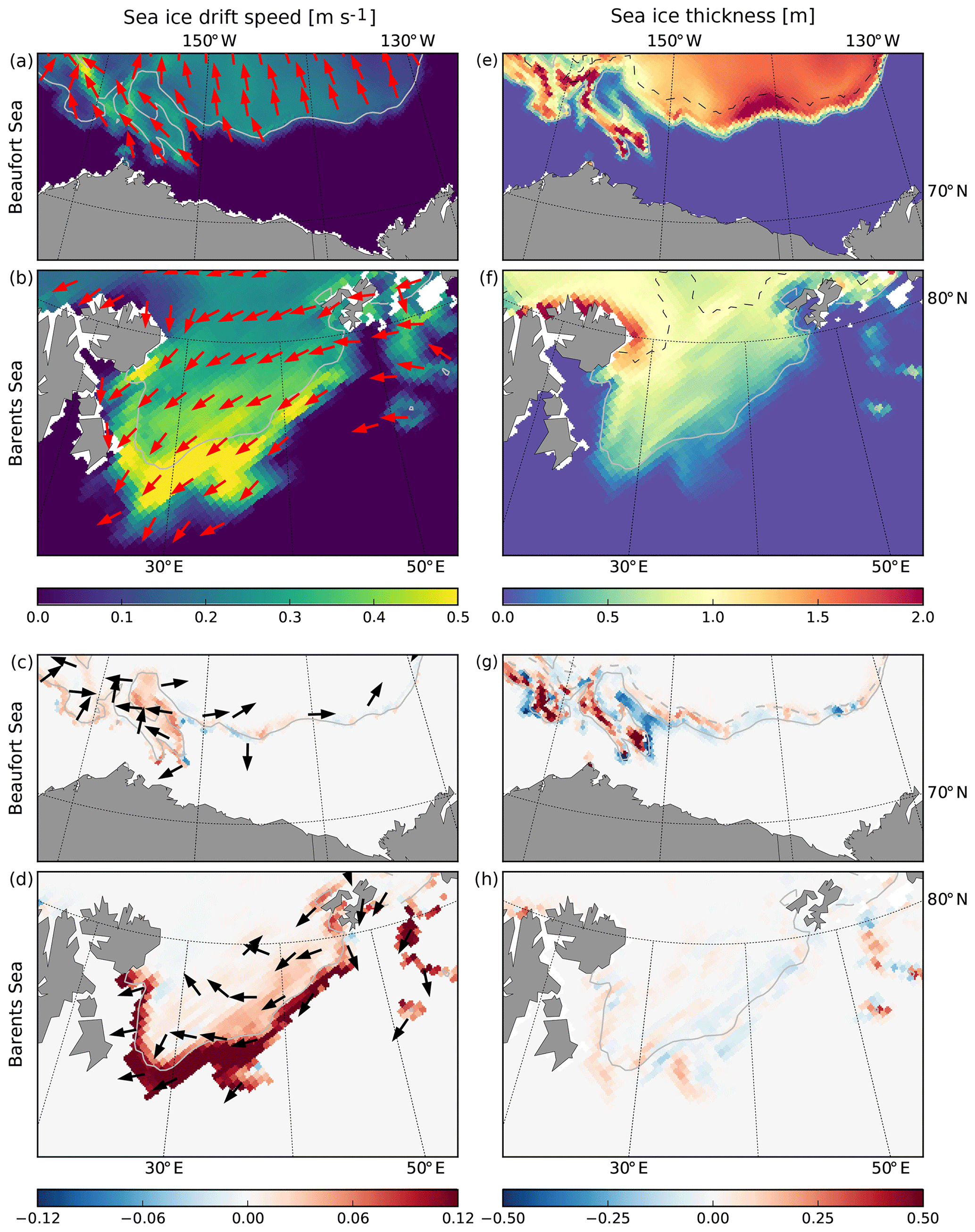
Figure 12Mean sea ice drift (a, b) and sea ice thickness (e, f) simulated by the CPL run during the storms that occurred in the Beaufort Sea (a, e) and in the Barents Sea (b, f) on 16–17 August 2010. Panels (c, d, g, h) show the differences for these quantities between the CPL and NOT_CPL simulations. Grey contours indicate the position of the ice edge determined from the averaged sea ice concentration (c=0.15). The dashed black contour delimits the border between broken and unbroken ice ( m).
4.2.2 Case 2 – storm in the Barents Sea (16–17 August 2010)
The storm that we just examined in the Beaufort Sea occurred on the same date as a second and stronger storm in the Barents Sea, with wave heights of up to 5 m and south-westerly winds reaching ≃ 15 m s−1 on average over the 2 d (Fig. 11d, e). In the CPL run, waves fragment sea ice over a very large area (Fig. 12f). Similarly to what we see in the Beaufort Sea, the mean direction of propagation of the waves aligns with the direction of the wind over the ice-free ocean and is rotated orthogonally to the gradient in sea ice thickness once in the sea ice pack (Fig. 11d). The transition is however much smoother here than in the Beaufort Sea as the gradient is much weaker (Fig. 12f). In the CPL run, sea ice is drifting southward (Fig. 12b), with a slight deviation from the wind direction and speeds twice as high as in the Beaufort Sea, due to stronger winds and thinner and less concentrated sea ice.
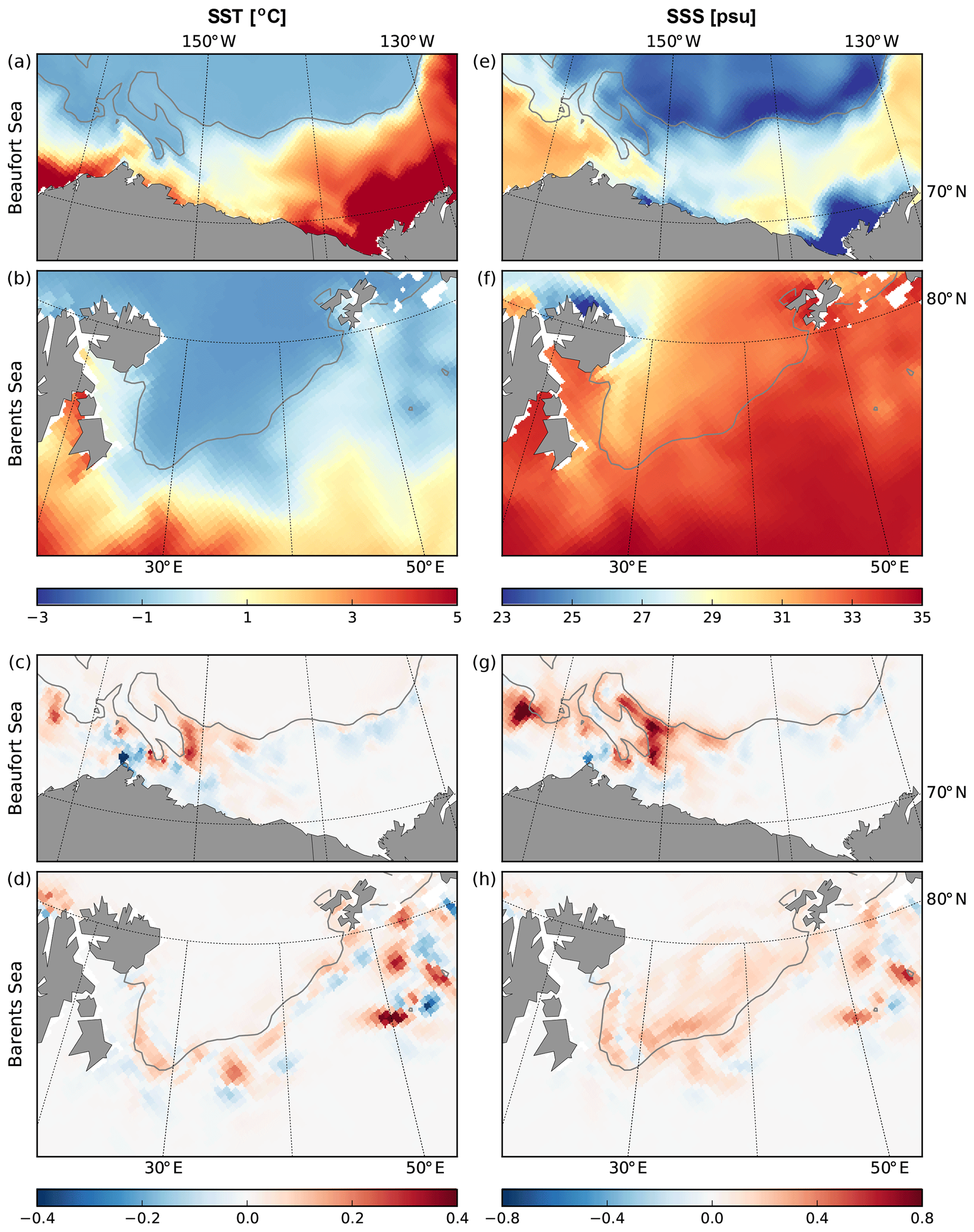
Figure 13SST (a, b) and SSS (e, f) simulated by the CPL run during the storms that occurred in the Beaufort Sea (a, e) and in the Barents Sea (b, f) on 16–17 August 2010. Panels (c, d, g, h) show the differences for these quantities between the CPL and NOT_CPL simulations. Grey contours indicate the position of the ice edge determined from the averaged sea ice concentration (c=0.15).
In contrast to the effects of the storm in the Beaufort Sea, the WRS in the CPL run reaches large values (Fig. 11f). Indeed, the strong storm generates high waves, inducing a WRS as large as the wind stress close to the sea ice edge where most of the attenuation takes place, although the WRS does not align with the direction of the wave propagation in ice. This is due to the low sea ice concentration in this region that allows for wave generation over a large region, even if partially ice-covered. The attenuation of these short in-ice-generated waves dominates the WRS that is therefore aligned with the wind direction, thus accelerating the ice drift, especially close to the ice edge (Fig. 12d).
The differences in sea ice drift between the CPL and the NOT_CPL runs also result in differences in bottom melt (Fig. 14d) and more specifically in the part associated with the turbulent heat flux (not shown). This increase in the turbulent heat flux, which occurs in the Barents Sea but not in the Beaufort Sea, can be explained by the larger ice drift velocities driven by the WRS, which intensify the shear between the sea ice and the ocean and therefore the turbulence in the surface mixed layer. The differences in sea ice drift between the two runs also result in changes in the conductive heat flux. However, in the Barents Sea, the sea ice thickness and concentrations are lower than in the Beaufort Sea, while the sea ice temperature is higher overall (not shown). This results in only moderate differences of the conductive heat flux between the CPL and NOT_CPL runs.
The differences in SST and SSS exhibit similar patterns to the differences in heat flux (Figs. 13d, h and 14c), but the magnitude of the differences is much weaker than in the Beaufort Sea, not exceeding a few tenths of a degree Celsius and practical salinity units for SST and SSS, respectively. These small differences can be explained by two causes: (i) the small differences of sea ice properties between the two simulations result in small changes in melt and (ii) the initial state before the storm is also different with higher SST and SSS in CPL (not shown). This difference in the initial state can be related to previous wave and wind conditions: low wind speeds are not sufficient to generate waves in the MIZ, implying that the WRS must be directed northward in the same direction as the propagating waves. It therefore compacts the sea ice edge and thus reduces sea ice melt in the MIZ in the CPL run. As seen in the Beaufort Sea case, this in turn leads to higher SST and SSS values in the vicinity of the ice edge.

Figure 14Averaged differences between the CPL and NOT_CPL simulations of (a, c) the heat flux into the ocean and (b, d) the contribution to the heat flux into the ocean coming from the sea ice bottom melt during the storms in the Beaufort Sea (a, b) and in the Barents Sea (c, d) which occurred on 16–17 August 2010. Grey contours indicate the position of the ice edge determined from the averaged sea ice concentration (c=0.15).
4.2.3 What determines the impact of the waves?
From these two particular cases we suggest a generalization of the mechanisms by which the waves can impact the sea ice and ocean properties in the MIZ. It is based on a simple principle: if sea ice is moved towards warmer water, it tends to melt more, and vice versa. The direction of the WRS compared to the orientation of the sea ice edge is thus fundamental if we are to understand the impact of the waves. In compact sea ice, waves are quickly attenuated and the direction of the WRS is generally towards the packed ice, thus impeding part of the sea ice melt and increasing the SST and SSS (Fig. 9). In regions where the sea ice is less concentrated and thinner, waves can be generated locally so that the WRS aligns with the wind, whose direction determines the impact of the WRS (enhanced melt for off-ice wind and reduced melt for on-ice wind). Another key factor determining the impact of the WRS on sea ice is the internal stress of sea ice (a.k.a. the rheology; see Eq. 2). The impact of the WRS is larger in regions of the MIZ where the sea ice is thin and has low concentration, as the internal stress tends to be negligible (Hibler III, 1979), making the sea ice easier to deform and to drift freely. Close to the sea ice edge in the Barents Sea for instance, the WRS in storm-induced high-wave conditions can be larger than the wind stress, strongly accelerating the sea ice drift towards the open ocean, which also results in an increase in the ice–ocean shear, enhancing the turbulent heat flux under sea ice and thus the sea ice melt.
The goal of this study was to examine the wave–sea ice interactions in the MIZ of the Arctic Ocean during the melt season as these processes are thought to be important for determining the sea ice conditions but are not accounted for in the state-of-the-art sea ice models. To that aim, we have developed a model framework, coupling the wave model WW3 with a modified version of the ocean–sea ice model NEMO-LIM3. The coupled model was then used to examine two aspects of the wave–sea ice interactions: (i) the impact of the WRS on the sea ice drift in the MIZ and (ii) the effects of using the wave-induced sea ice fragmentation to estimate lateral melt. The WRS tends to compact the ice edge and thus reduces the total sea ice melt in the MIZ. Yet, its overall impact on the MIZ sea ice area and volume remains limited (Fig. 8b). However, it has a visible impact on sea ice drift velocity, accelerating it by ≃ 9 %. Compared to the use of the parameterization of Lüpkes et al. (2012) to estimate the floe size used in lateral melt, our parameterization strongly reduces the amount of sea ice melted laterally. It is however mostly compensated by an increase in bottom melt, similar to what was found by Bateson et al. (2019). As a result, the effects on sea ice and sea surface properties can be locally substantial and even more substantial during storms, as illustrated by the case studies in the Beaufort and Barents seas. As the storminess in the Arctic region is expected to increase in the future (Day et al., 2018; Day and Hodges, 2018), generating higher and more energetic waves more frequently (Khon et al., 2014), the wave–sea ice interactions might become a dominant signal controlling the dynamics of the MIZ.
In the MIZ, waves push sea ice as they are attenuated, locally modifying the position of the sea ice edge through a modulation of the magnitude and timing of the sea ice melt, which results in significant changes in the SST and SSS. Although the impact at the pan-Arctic scale remains limited, the case studies of storms in the Barents and Beaufort seas show how this modulation can be locally and intermittently important. Results from our simple configuration have also revealed that the WRS could strongly modulate the position of the sea ice edge. Yet, except very locally in response to strong storms, the position of the pan-Arctic sea ice edge simulated by our realistic configuration appears to be insensitive to the effect of the wave. This is likely because the position of the sea ice edge in an ocean–sea ice model is primarily determined by the atmospheric forcing and the bulk formulae and is in particular strongly tied to the position of the sea ice edge in the atmospheric reanalysis (Chevallier et al., 2017). The effects of the waves on sea ice simulated by our coupled model are likely underestimated and should be reassessed in future studies based on a fully coupled model that includes an atmospheric component.
We have also tested two parameterizations of the lateral melt, based either on wave-induced fragmentation information or solely on a scaling between the size of the floes and the sea ice concentration, following Lüpkes et al. (2012). We first acknowledge that the effect of our lateral-melt parameterization depends strongly on the FSD and hence on the choices and assumptions made regarding its implementation. For instance, our redistribution scheme associated with sea ice fragmentation assumes that successive fragmentation events lead to a power-law FSD. This assumption is made based on the observations analysed by Toyota et al. (2011) that only sample a small area in time and space, and their findings may not be applicable globally. More generally, Roach et al. (2018b) recommend avoiding forcing the shape of the distribution, as the analysis of observations has revealed that FSDs do not always follow power-law distributions (e.g. Inoue et al., 2004). They (i.e. Roach et al., 2018b) foster the use of alternative approaches, such as the one developed by Horvat and Tziperman (2015). However, results from laboratory experiments focusing on the fragmentation of sea ice by waves by Herman et al. (2018) indeed suggest power-law distributions for the smallest floe sizes generated, similar to what was found by Toyota et al. (2011) for the small-floes regime. This justifies the choice made in the present study. More generally, large uncertainty remains regarding the key parameters governing the FSD redistribution (coming from waves or sea ice properties), and more dedicated observations will be needed in the future to better constrain the FSD in models.
Regardless of the choices made for the implementation of the FSD, the effect of the lateral melt for both formulations remains limited as any change in lateral melt tends to be compensated for by an opposite change in bottom melt. The effect might however become more important if longer simulations were performed. Indeed, Zhang et al. (2016) found that, over a year, the lateral melt could significantly affect the sea ice thickness. In their case, an FSD-based parameterization was used (similar to the one we introduced in our coupled model), but the effect of the wave-induced fragmentation on the FSD was only crudely parameterized, resulting most likely in an overestimation of lateral melt in the central Arctic (as this is the case when using the parameterization of Lüpkes et al., 2012). Adding an FSD to their sea ice model, Roach et al. (2018b) found a large impact on sea ice concentration in the MIZ and sea ice thickness everywhere in the Arctic after 20 years of simulation and suggested that the differences found in the central Arctic result from a redistribution of the heat used for lateral melt instead of bottom melt, similar to what happens in our model over a shorter timescale. One should also remember that the studies of Zhang et al. (2016) and Roach et al. (2018b) aimed to represent the evolution of floes with sizes ranging from a few centimetres to roughly 1 km on long timescales, whereas we focus on the important processes for wave–sea ice interactions and make the assumption that unbroken floes have a uniform floe size set to 1000 m. Therefore we do not expect any impact of the lateral melt in regions that are not impacted by waves. Note also that we evaluate the impact of changing the lateral-melt parameterization by comparing two simulations for which lateral melt depends on a varying floe size, either deduced from the FSD or estimated from the sea ice concentration using the parameterization suggested in Lüpkes et al. (2012). It differs from Zhang et al. (2016), who compare their FSD model with a reference run without lateral melt, and from Roach et al. (2018b), who use a constant floe size of 300 m in their lateral-melt parameterization. This might partly explain the discrepancies between our respective conclusions.
Among the wave–sea ice interaction processes considered in this study, we find that the dynamical effect of the waves (the WRS) has a larger impact on sea ice conditions and sea surface properties than the modulation of lateral melt by sea ice fragmentation. Our simulations were however limited to only a few weeks during the melting season, and it is unclear if the result would hold if longer timescales were considered. In order to answer this question, we would need to implement a parameterization that accounts for the refreezing of floes, through lateral growth and welding. A first parameterization of this kind has been very recently developed by Roach et al. (2018b). We also anticipate that running a simulation over longer time periods would highlight new impacts of the WRS. Indeed, observations have revealed that heat stored during the melt season below the mixed layer can significantly affect sea ice growth the following year (Jackson et al., 2010; Timmermans, 2015). In regions where the WRS contributes to reducing the ice melt, an excess of summer heat could likely accumulate under the mixed layer, possibly modulating the future evolution of the sea ice melt and growth. Recently, Smith et al. (2018), for instance, observed that a large amount of heat stored under the mixed layer could be released to melt sea ice during a storm. The significant changes in SST and SSS found locally over 37 d also highlight that wave–sea ice interactions should be considered when trying to forecast the Arctic sea ice conditions on short timescales (up to a few weeks), as these surface ocean changes can greatly affect melting and refreezing conditions.
The coupling developed in this study marks a valuable new step towards an improved representation of waves and sea ice interactions in models, which might improve the representation of the dynamics in the MIZ. Yet, our coupling relies on a number of assumptions, which are most likely leading to an underestimation of the impact of the waves on the ocean and sea ice conditions. For instance, in our coupling, the sea ice rheology is unaffected by fragmentation, which is unlikely to be the case in reality (McPhee, 1980). Moreover, the sea ice model used here does not retain any memory of the past sea ice conditions, while waves would most likely have a different effect on sea ice that has been previously broken (Langhorne et al., 1998). Developing a similar coupling using a model that considers a state variable accounting for the previous sea ice conditions (such as in the neXtSIM sea ice model; Rampal et al., 2016; Williams et al., 2017) would probably reveal new mechanisms via which waves can modulate the ocean and sea ice conditions in the MIZ. Finally, the coupling we have developed here also only considers the interactions between waves and sea ice, without any direct coupling with the ocean and the atmosphere. Yet, we know that wave dissipation would also likely impact the mixed layer, by enhancing turbulence (Couvelard et al., 2019), and eventually modulate the rate of sea ice melt and formation (Martin and Kauffman, 1981; Rainville et al., 2011; Lee et al., 2012; Smith et al., 2018). Similarly, the effect of the waves is probably dampened due to the lack of feedbacks with the atmosphere (Khon et al., 2014). Future coupling should include some of these features in order to fully capture the complexity of the MIZ dynamics.
Here we provide the details of the calculation and implementation of the FSD and in particular of the mechanical redistribution function Φm that accounts for processes such as sea ice fragmentation, lead opening, ridging and rafting. Following Zhang et al. (2015), Φm can be divided into three terms as , where Φo represents the creation of open water, Φr represents sea ice ridging and rafting, and Φf represents the wave-induced floe fragmentation. Here we compute Φo and Φr in a similar way to Zhang et al. (2015), assuming that all the floes of different sizes have the same ice thickness distribution so that changes in sea ice concentration due to open water creation or ridging affect all floes equally. As a result, the shape of the FSD and its evolution are independent from these two terms.
Assuming that, in a given grid cell, sea ice fragmentation does not induce any change in the sea ice concentration, Φf can be written as (Zhang et al., 2015)
where D is the floe size, Q(D) is a redistribution probability function characterizing which floes are going to be broken depending on their size and is a redistribution factor quantifying the fraction of sea ice concentration transferred from one floe size to another as fragmentation occurs. Thus Φf is used to transfer sea ice concentration from large floes to smaller floes. To ensure the conservation of sea ice area during fragmentation, β must respect (Zhang et al., 2015)
In the absence of a wave model to simulate the sea state, Zhang et al. (2015) defined β so that it uniformly redistributes the sea ice concentration of the large broken floes into the smaller floe size categories of the FSD. Their redistribution probability function Q(D) thus assumes that a constant fraction of the sea ice cover is broken by waves during each fragmentation event. Their definition of Q(D) also ensures that larger floes contribute more to the redistribution than smaller floes.
In our coupled model, sea ice fragmentation is initially computed by WW3 (for details see Boutin et al., 2018) and accounts for the sea state variability. In WW3, the FSD resulting from wave-induced fragmentation is assumed to follow a truncated power law between a minimum (Dmin) and a maximum (Dmax) floe size. For consistency, the FSD in LIM3 after a given fragmentation event must follow the same power law, defined for D taken in [Dmin, Dmax] such as, for a given floe size D* also taken in [Dmin, Dmax],
where is the probability of having , and p(D) is the associated probability density. In WW3, a fragmentation event occurs if two conditions are met: (i) waves with a wavelength λ apply a strain on sea ice greater than a given threshold and (ii) λ∕2, which is assumed to be the value of the new maximum floe size, is lower than the current Dmax value in the wave model (Dumont et al., 2011). Therefore, a fragmentation event in WW3 corresponds to a decrease in Dmax.
As detailed in Sect. 3.2, we define a maximum floe size in LIM3, Dmax,LIM3, that is compared to the value of the maximum floe size received from WW3, Dmax,WW3 . Initially, ice is unbroken and . If fragmentation has occurred in WW3, then we have . In this case, Dmax,LIM3 must be updated to the Dmax,WW3 value, and Φf must be computed so that it forces the FSD in LIM3 to match the FSD assumed in WW3.
In practice, in LIM3, we define a given number N of floe size categories, such that each floe size category represents the floes with sizes in [Dn−1, Dn]. D0 and DN are the minimum and the maximum floe size possible in the model, respectively. DN aims to represent floes that have not been broken by the waves. In WW3, the size of unbroken floes is set to 1000 m, and we thus also set DN=1000 m for consistency. Regarding the minimum floe size resulting from wave-induced fragmentation, we set Dmin to 8 m, which is the value of the minimum floe size used in the parameterization of lateral melt implemented in LIM3. This value is close to choices made in previous studies (see Williams et al., 2013; Bennetts et al., 2017). If fragmentation occurs, the update of Dmax,LIM3 is carried out as follows:
Here n* is the index of the floe size category in which the maximum floe size received from the wave model lies. Dmax,LIM3, the maximum floe size in the sea ice model, is thus set equal to , the upper bound of the n*th category. To force the FSD to follow this power law during the computation of the mechanical redistribution term Φf, in LIM3 we introduce changes in the computation of β and Q(D). When using N floe size categories, the redistribution equation (Eq. A1) becomes
Following Zhang et al. (2015), the redistribution factor β(m,n) must respect Eq. (A2). It, β(m,n), should also allow for a switch from completely unbroken ice to a truncated power-law distribution with lower limit D0 and upper limit Dmax,LIM3 if fragmentation occurs. Finally, β(m,n) must ensure that floe size can only decrease during the fragmentation. To do so, β(m,n) is defined as
With this choice of β(m,n), the FSD of each floe size category is equal to the distribution function derived from the power law assumed in WW3 (), given by
c being the sea ice concentration.
If sea ice in a given grid cell has already been broken, the FSD may have deviated from the truncated power-law distribution (due to advection or melting). If fragmentation occurs again at a later model time step, we force the FSD to be reset to the power law assumed in WW3, by adjusting the fraction of each floe size category contributing to the redistribution through the value Qn. This ensures that the FSDs in LIM3 and WW3 are identical. After a fragmentation event, Dmax,LIM3 is the new maximum floe size in LIM3. The sea ice contained in floe size categories associated with floes larger than Dmax,LIM3 is therefore entirely redistributed into smaller floe size categories by setting
The smallest floe size category (i.e. ) does not contribute to the floe size redistribution, assuming that this category accounts for floes too small to be broken by waves (Toyota et al., 2011). It therefore forces Q1=0. For a given floe size category n, we define Δgth,n as the difference between the actual and theoretical values of the FSD for this floe size category (), and the theoretical value is given by the truncated power law between D0 and Dmax,LIM3. After the redistribution of floes between categories, Δgth,n needs to be zero, which is achieved through the adjustment of Qn in order to obtain . The following system thus needs to be solved:
This system consists in a triangular matrix in which all diagonal terms are non-zero. It is solved by carrying out
The constraint Qn>0 ensures that the redistribution can only be performed towards categories containing smaller floe sizes. This constraint thus implies that, in the case where , the FSD in LIM3 is reset to the truncated power law only if there is enough sea ice in large floe categories to be redistributed into smaller floe categories. Besides, setting Q1=0 means that the sea ice concentration associated with the smallest floe size category is never redistributed. In the absence of lateral growth, a succession of fragmentation events leads to an accumulation of floes in this category, deviating the FSD from the theoretical power law for floe sizes between D0 and D1 (see Fig. 3).
The Drakkar forcing set is described in Brodeau et al. (2010) and is freely available at: https://ige-meom-opendap.univ-grenoble-alpes.fr/thredds/catalog/meomopendap/extract/FORCING_ATMOSPHERIQUE/DFS5.2/ALL/catalog.html (last access: January 2020). The wave–sea ice coupling routines developed in WW3 are included in the publicly available latest release of the code (v6.07) at: https://github.com/NOAA-EMC/WW3 (last access: December 2019, WW3DG, 2019). The modified routines of NEMO-LIM3 allowing for the wave–sea ice coupling are available at: https://doi.org/10.5281/zenodo.3600149 (Boutin et al., 2020). Configuration files are available upon request from claude.talandier@ifremer.fr or camille.lique@ifremer.fr. Model outputs are available upon request from guillaume.boutin@nersc.no.
GB and FA formulated the study. GB, FA, CR, CT and CL developed the coupled framework. GB and CL led the paper writing with significant input from the other authors.
The authors declare that they have no conflict of interest.
Part of this work has been carried out as part of the Copernicus Marine Environment Monitoring Service (CMEMS) ArcticMix and WIzARd projects. CMEMS is implemented by Mercator Ocean in the framework of a delegation agreement with the European Union. We thank Martin Vancoppenolle for his valuable help as well as Verena Haid and Xavier Couvelard for their significant assistance in setting up the coupled framework.
This research has been supported by the DGA, the ANR (grant nos. ANR-14-CE01-0012 MIMOSA and ANR-10-LABX-19-01), the EU-FP7 (grant no. SWARP 607476), the ONR (grant no. N0001416WX01117), and the CMEMS (grant projects ArcticMix and WIzARd).
This paper was edited by Daniel Feltham and reviewed by three anonymous referees.
Aksenov, Y., Popova, E. E., Yool, A., Nurser, A. G., Williams, T. D., Bertino, L., and Bergh, J.: On the future navigability of Arctic sea routes: High-resolution projections of the Arctic Ocean and sea ice, Mar. Policy, 75, 300–317, 2017. a
Ardhuin, F., Sutherland, P., Doble, M., and Wadhams, P.: Ocean waves across the Arctic: attenuation due to dissipation dominates over scattering for periods longer than 19 s, Geophys. Res. Lett., 43, 5775–5783, https://doi.org/10.1002/2016GL068204, 2016. a
Ardhuin, F., Chapron, B., Collard, F., Smith, M., Stopa, J., Thomson, J., Doble, M., Wadhams, P., Blomquist, B., Persson, O., and Collins, III, C. O.: Measuring ocean waves in sea ice using SAR imagery: A quasi-deterministic approach evaluated with Sentinel-1 and in situ data, Remote Sens. Environ., 189, 211–222, 2017. a
Ardhuin, F., Boutin, G., Stopa, J., Girard-Ardhuin, F., Melsheimer, C., Thomson, J., Kohout, A., Doble, M., and Wadhams, P.: Wave Attenuation Through an Arctic Marginal Ice Zone on October 12, 2015: 2. Numerical modeling of Waves and Associated Ice Break-Up, J. Geophys. Res.-Oceans, 123, 5652–5668, https://doi.org/10.1002/2018JC013784, 2018. a, b, c, d, e
Asplin, M. G., Galley, R., Barber, D. G., and Prinsenberg, S.: Fracture of summer perennial sea ice by ocean swell as a result of Arctic storms, J. Geophys. Res., 117, C06025, https://doi.org/10.1029/2011JC007221, 2012. a
Barnier, B., Madec, G., Penduff, T., Molines, J.-M., Treguier, A.-M., Sommer, J. L., Beckmann, A., Biastoch, A., Böning, C., Dengg, J., Derval, C., Durand, E., Gulev, S., Remy, E., Talandier, C., Theetten, S., Maltrud, M., McClean, J., and Cuevas, B. D.: Impact of partial steps and momentum advection schemes in a global ocean circulation model at eddy-permitting resolution, Ocean Model., 56, 543–567, https://doi.org/10.1007/s10236-006-0082-1, 2006. a
Bateson, A. W., Feltham, D. L., Schröder, D., Hosekova, L., Ridley, J. K., and Aksenov, Y.: Impact of floe size distribution on seasonal fragmentation and melt of Arctic sea ice, The Cryosphere Discuss., https://doi.org/10.5194/tc-2019-44, in review, 2019. a, b, c
Bennetts, L. G., O'Farrell, S., and Uotila, P.: Brief communication: Impacts of ocean-wave-induced breakup of Antarctic sea ice via thermodynamics in a stand-alone version of the CICE sea-ice model, The Cryosphere, 11, 1035–1040, https://doi.org/10.5194/tc-11-1035-2017, 2017. a, b
Bouillon, S., Fichefet, T., Legat, V., and Madec, G.: The elastic–viscous–plastic method revisited, Ocean Model., 71, 2–12, https://doi.org/10.1016/j.ocemod.2013.05.013, 2013. a
Boutin, G., Ardhuin, F., Dumont, D., Sévigny, C., Girard-Ardhuin, F., and Accensi, M.: Floe Size Effect on Wave-Ice Interactions: Possible Effects, Implementation in Wave Model, and Evaluation, J. Geophys. Res.-Oceans, 123, 4779–4805, https://doi.org/10.1029/2017JC013622, 2018. a, b, c, d, e, f, g, h
Boutin, G.: gboutin-lops/nemo_lim3_wave_ice_cpl: TC_code (Version v1.0), Zenodo, https://doi.org/10.5281/zenodo.3600149, 2020. a
Brodeau, L., Barnier, B., Treguier, A.-M., Penduff, T., and Gulev, S.: An ERA40-based atmospheric forcing for global ocean circulation models, Ocean Model., 31, 88–104, 2010. a, b
Cheng, S., Rogers, W. E., Thomson, J., Smith, M., Doble, M. J., Wadhams, P., Kohout, A. L., Lund, B., Persson, O. P., Collins, C. O., Ackley, S. F., Montiel, F., and Shen, H. H.: Calibrating a viscoelastic sea ice model for wave propagation in the arctic fall marginal ice zone, J. Geophys. Res.-Oceans, 122, 8770–8793, 2017. a
Chevallier, M., Smith, G. C., Dupont, F., Lemieux, J.-F., Forget, G., Fujii, Y., Hernandez, F., Msadek, R., Peterson, K. A., Storto, A., Toyoda, T., Valdivieso, M., Vernieres, G., Zuo, H., Balmaseda, M., Chang, Y.-S., Ferry, N., Garric, G., Haines, K., Keeley, S., Kovach, R. M., Kuragano, T., Masina, S., Tang, Y., Tsujino, H., and Wang, X.: Intercomparison of the Arctic sea ice cover in global ocean–sea ice reanalyses from the ORA-IP project, Climate Dynam., 49, 1107–1136, 2017. a, b
Collins, III, C. O., Rogers, W. E., Marchenko, A., and Babanin, A. V.: In situ measurements of an energetic wave event in the Arctic marginal ice zone, Geophys. Res. Lett., 42, 1863–1870, https://doi.org/10.1002/2015GL063063, 2015. a, b
Comiso, J. C., Meier, W. N., and Gersten, R.: Variability and trends in the Arctic Sea ice cover: Results from different techniques, J. Geophys. Res.-Oceans, 122, 6883–6900, 2017. a
Couvelard, X., Lemarié, F., Samson, G., Redelsperger, J.-L., Ardhuin, F., Benshila, R., and Madec, G.: Development of a 2-way coupled ocean-wave model: assessment on a global NEMO(v3.6)-WW3(v6.02) coupled configuration, Geosci. Model Dev. Discuss., https://doi.org/10.5194/gmd-2019-189, in review, 2019. a
Craig, A., Valcke, S., and Coquart, L.: Development and performance of a new version of the OASIS coupler, OASIS3-MCT_3.0, Geosci. Model Dev., 10, 3297–3308, https://doi.org/10.5194/gmd-10-3297-2017, 2017. a
Day, J. J. and Hodges, K. I.: Growing land-sea temperature contrast and the intensification of Arctic cyclones, Geophys. Res. Lett., 45, 3673–3681, 2018. a
Day, J. J., Holland, M. M., and Hodges, K. I.: Seasonal differences in the response of Arctic cyclones to climate change in CESM1, Clim. Dynam., 50, 3885–3903, 2018. a
Dumont, D., Kohout, A., and Bertino, L.: A wave-based model for the marginal ice zone including a floe breaking parameterization, J. Geophys. Res., 116, C00E03, https://doi.org/10.1029/2010JC006682, 2011. a, b, c, d, e
Dupont, F., Higginson, S., Bourdallé-Badie, R., Lu, Y., Roy, F., Smith, G. C., Lemieux, J.-F., Garric, G., and Davidson, F.: A high-resolution ocean and sea-ice modelling system for the Arctic and North Atlantic oceans, Geosci. Model Dev., 8, 1577–1594, https://doi.org/10.5194/gmd-8-1577-2015, 2015. a
Feltham, D. L.: Granular flow in the marginal ice zone, Philos. T. R. Soc. Lond, 363, 1677–1700, 2005. a
Herman, A., Evers, K.-U., and Reimer, N.: Floe-size distributions in laboratory ice broken by waves, The Cryosphere, 12, 685–699, https://doi.org/10.5194/tc-12-685-2018, 2018. a, b
Hibler III, W. D.: A Dynamic Thermodynamic Sea Ice Model, J. Phys. Oceanogr., 9, 815–846, https://doi.org/10.1175/1520-0485(1979)009<0815:ADTSIM>2.0.CO;2, 1979. a, b
Horvat, C. and Tziperman, E.: A prognostic model of the sea-ice floe size and thickness distribution, The Cryosphere, 9, 2119–2134, https://doi.org/10.5194/tc-9-2119-2015, 2015. a, b, c, d, e, f
Hunke, E. C. and Dukowicz, J. K.: An Elastic–Viscous–Plastic Model for Sea Ice Dynamics, J. Phys. Oceanogr., 27, 1849–1867, https://doi.org/10.1175/1520-0485(1997)027<1849:AEVPMF>2.0.CO;2, 1997. a
Inoue, J., Wakatsuchi, M., and Fujiyoshi, Y.: Ice floe distribution in the Sea of Okhotsk in the period when sea-ice extent is advancing, Geophys. Res. lett., 31, L20303, https://doi.org/10.1029/2004GL020809, 2004. a
Jackson, J., Carmack, E., McLaughlin, F., Allen, S. E., and Ingram, R.: Identification, characterization, and change of the near-surface temperature maximum in the Canada Basin, 1993–2008, J. Geophys. Res.-Oceans, 115, C05021, https://doi.org/10.1029/2009JC005265, 2010. a
Khon, V., Mokhov, I., Pogarskiy, F., Babanin, A., Dethloff, K., Rinke, A., and Matthes, H.: Wave heights in the 21st century Arctic Ocean simulated with a regional climate model, Geophys. Res. Lett., 41, 2956–2961, 2014. a, b
Kohout, A. L., Williams, M. J. M., Dean, S. M., and Meylan, M. H.: Storm-induced sea-ice breakup and the implications for ice extent, Nature, 509, 604–607, https://doi.org/10.1038/nature13262, 2014. a
Langhorne, P. J., Squire, V. A., Fox, C., and Haskell, T. G.: Break-up of sea ice by ocean waves, Ann. Glaciol., 27, 438–442, 1998. a, b
Lee, C. M., Cole, S., Doble, M., Freitag, L., Hwang, P., Jayne, S., Jeffries, M., Krishfield, R., Maksym, T., and Maslowski, W.: Marginal Ice Zone (MIZ) program: Science and experiment plan, Tech. rep., Washington Univ Seattle Applied Physics Lab, 2012. a, b
Lemieux, J.-F., Lei, J., Dupont, F., Roy, F., Losch, M., Lique, C., and Laliberté, F.: The Impact of Tides on Simulated Landfast Ice in a Pan-Arctic Ice-Ocean Model, J. Geophys. Res.-Oceans, 123, 7747–7762, 2018. a
Lique, C., Holland, M. M., Dibike, Y. B., Lawrence, D. M., and Screen, J. A.: Modeling the Arctic freshwater system and its integration in the global system: Lessons learned and future challenges, J. Geophys. Res.-Biogeo., 121, 540–566, 2016. a
Longuet-Higgins, M. S.: The mean forces exerted by waves on floating or submerged bodies with applications to sand bars and wave power machines, Proc. Roy. Soc. Lond. A, 352, 463–480, 1977. a, b
Longuet-Higgins, M. S. and Stewart, R. W.: Radiation stresses and mass transport in surface gravity waves with application to `surf beats', J. Fluid Mech., 13, 481–504, 1962. a
Lüpkes, C., Gryanik, V. M., Hartmann, J., and Andreas, E. L.: A parametrization, based on sea ice morphology, of the neutral atmospheric drag coefficients for weather prediction and climate models, J. Geophys. Res.-Atmos., 117, D13112, https://doi.org/10.1029/2012JD017630, 2012. a, b, c, d, e, f, g, h, i, j, k, l, m, n, o, p, q, r, s
Madec, G.: NEMO ocean engine, Note du Pôle de modélisation, Institut Pierre-Simon Laplace (IPSL), France, No. 27, ISSN: 1288-1619, 2008. a
Marcq, S. and Weiss, J.: Influence of sea ice lead-width distribution on turbulent heat transfer between the ocean and the atmosphere, The Cryosphere, 6, 143–156, https://doi.org/10.5194/tc-6-143-2012, 2012. a
Martin, S. and Kauffman, P.: A Field and Laboratory Study of Wave Damping by Grease Ice, J. Glaciol., 27, 283–313, https://doi.org/10.1017/S0022143000015392, 1981. a
Maykut, G. A. and Perovich, D. K.: The role of shortwave radiation in the summer decay of a sea ice cover, J. Geophys. Res.-Oceans, 92, 7032–7044, 1987. a
McPhee, M. G.: An analysis of pack ice drift in summer, Sea ice processes and models, University of Washington Press Seattle, 62–75, 1980. a, b
Mellor, M.: Mechanical Behavior of Sea Ice, in: The Geophysics of SeaIce, edited by: Untersteiner, N., NATO ASI Series, Springer US, 165–281, https://doi.org/10.1007/978-1-4899-5352-0_3, 1986. a
Montiel, F., Squire, V. A., and Bennetts, L. G.: Attenuation and directional spreading of ocean wave spectra in the marginal ice zone, J. Fluid Mech., 790, 492–522, https://doi.org/10.1017/jfm.2016.2, 2016. a
Perrie, W. and Hu, Y.: Air–ice–ocean momentum exchange – Part II: Ice drift, J. Phys. Oceanogr., 27, 1976–1996, https://doi.org/10.1175/1520-0485(1997)027<1976:AIOMEP>2.0.CO;2, 1997. a
Rainville, L., Lee, C. M., and Woodgate, R. A.: Impact of wind-driven mixing in the Arctic Ocean, Oceanography, 24, 136–145, 2011. a
Rampal, P., Bouillon, S., Ólason, E., and Morlighem, M.: neXtSIM: a new Lagrangian sea ice model, The Cryosphere, 10, 1055–1073, https://doi.org/10.5194/tc-10-1055-2016, 2016. a, b
Roach, L. A., Dean, S. M., and Renwick, J. A.: Consistent biases in Antarctic sea ice concentration simulated by climate models, The Cryosphere, 12, 365–383, https://doi.org/10.5194/tc-12-365-2018, 2018a. a
Roach, L. A., Horvat, C., Dean, S. M., and Bitz, C. M.: An emergent sea ice floe size distribution in a global coupled ocean–sea ice model, J. Geophys. Res.-Oceans, 123, 4322–4337, 2018b. a, b, c, d, e, f, g, h, i, j
Rogers, W. E., Thomson, J., Shen, H. H., Doble, M. J., Wadhams, P., and Cheng, S.: Dissipation of wind waves by pancake and frazil ice in the autumn Beaufort Sea, J. Geophys. Res., 121, 7991–8007, https://doi.org/10.1002/2016JC012251, 2016. a
Rothrock, D. and Thorndike, A.: Measuring the sea ice floe size distribution, J. Geophys. Res.-Oceans, 89, 6477–6486, 1984. a, b
Rousset, C., Vancoppenolle, M., Madec, G., Fichefet, T., Flavoni, S., Barthélemy, A., Benshila, R., Chanut, J., Levy, C., Masson, S., and Vivier, F.: The Louvain-La-Neuve sea ice model LIM3.6: global and regional capabilities, Geosci. Model Dev., 8, 2991–3005, https://doi.org/10.5194/gmd-8-2991-2015, 2015. a, b
Shen, H. H. and Ackley, S. F.: A one-dimensional model for wave-induced ice-floe collisions, Ann. Glaciol., 15, 87–95, 1991. a
Smith, M., Stammerjohn, S., Persson, O., Rainville, L., Liu, G., Perrie, W., Robertson, R., Jackson, J., and Thomson, J.: Episodic reversal of autumn ice advance caused by release of ocean heat in the Beaufort Sea, J. Geophys. Res.-Oceans, 123, 3164–3185, 2018. a, b, c
Squire, V. A.: A fresh look at how ocean waves and sea ice interact, Phil. Trans. R. Soc. A, 376, 20170342, https://doi.org/10.1098/rsta.2017.0342, 2018. a
Steele, K., Teng, C.-C., and Wang, D. W.-C.: Wave direction measurements using pitch and roll buoys, Ocean Eng., 19, 349–375, 1992. a
Steele, M.: Sea ice melting and floe geometry in a simple ice-ocean model, J. Geophys. Res.-Oceans, 97, 17729–17738, https://doi.org/10.1029/92JC01755, 1992. a
Steele, M., Morison, J. H., and Untersteiner, N.: The partition of air-ice-ocean momentum exchange as a function of ice concentration, floe size, and draft, J. Geophys. Res.-Oceans, 94, 12739–12750, 1989. a
Stopa, J., Ardhuin, F., Thomson, J., Smith, M. M., Kohout, A., Doble, M., and Wadhams, P.: Wave Attenuation Through an Arctic Marginal Ice Zone on 12 October, 2015: 1. Measurement of Wave Spectra and Ice Features From Sentinel-1A, J. Geophys. Res.-Oceans, 123, 3619–3634, 2018a. a, b
Stopa, J. E., Ardhuin, F., and Girard-Ardhuin, F.: Wave climate in the Arctic 1992–2014: seasonality and trends, The Cryosphere, 10, 1605–1629, https://doi.org/10.5194/tc-10-1605-2016, 2016. a, b
Stopa, J. E., Sutherland, P., and Ardhuin, F.: Strong and highly variable push of ocean waves on Southern Ocean sea ice, P. Natl. Acad. Sci. USA, 115, 5861–5865, 2018b. a
Stroeve, J., Hamilton, L. C., Bitz, C. M., and Blanchard-Wrigglesworth, E.: Predicting September sea ice: Ensemble skill of the SEARCH Sea Ice Outlook 2008–2013, Geophys. Res. Lett., 41, 2411–2418, https://doi.org/10.1002/2014GL059388, 2014. a
Strong, C. and Rigor, I. G.: Arctic marginal ice zone trending wider in summer and narrower in winter, Geophys. Res. Lett., 40, 4864–4868, https://doi.org/10.1002/grl.50928, 2013. a, b
Sutherland, P. and Dumont, D.: Marginal ice zone thickness and extent due to wave radiation stress, J. Phys. Oceanogr., 48, 1885–1901, https://doi.org/10.1175/JPO-D-17-0167.1, 2018. a
Sutherland, P. and Melville, W. K.: Field measurements and scaling of ocean surface wave-breaking statistics, Geophys. Res. Lett., 40, 3074–3079, https://doi.org/10.1002/grl.50584, 2013. a
Thomson, J. and Rogers, W. E.: Swell and sea in the emerging Arctic Ocean, Geophys. Res. Lett., 41, 3136–3140, https://doi.org/10.1002/2014GL059983, 2014. a
Thomson, J., Ackley, S., Girard-Ardhuin, F., Ardhuin, F., Babanin, A., Bidlot, J., Boutin, G., Brozena, J., Cheng, S., Doble, M., Fairall, C. Guest, P., Gebhardt, C., Gemmrich, J., Graber, H. C., Holt, B., Lehner, S., Lund, B., Meylan, M. H., Maksym, T., Montiel, F., Perrie, W., Persson, O., Rainville, L., Rogers, W. E., Shen, H., Shen, H., Squire, V., Stammerjohn, S., Stopa, J., Smith, M. M., Sutherland, P., and Wadhams P.: Overview of the arctic sea state and boundary layer physics program, J. Geophys. Res.-Oceans, 123, 8674–8687, 2018. a, b
Timmermans, M.-L.: The impact of stored solar heat on Arctic sea ice growth, Geophys. Res. Lett., 42, 6399–6406, 2015. a
Toyota, T., Haas, C., and Tamura, T.: Size distribution and shape properties of relatively small sea-ice floes in the Antarctic marginal ice zone in late winter, Deep-Sea Res. Pt. II, 58, 1182–1193, 2011. a, b, c, d, e, f
Tsamados, M., Feltham, D., Petty, A., Schroeder, D., and Flocco, D.: Processes controlling surface, bottom and lateral melt of Arctic sea ice in a state of the art sea ice model, Philos. T. R. Soc. Lond, 373, 20140167, https://doi.org/10.1098/rsta.2014.0167, 2015. a
Uotila, P., Goosse, H., Haines, K., Chevallier, M., Barthélemy, A., Bricaud, C., Carton, J., Fučkar, N., Garric, G., Iovino, D., Kauker, F., Korhonen, M., Lien, V. S., Marnela, M., Massonnet, F., Mignac, D., Peterson, K. A., Sadikni, R., Shi, L., Tietsche, S., Toyoda, T., Xie, J., and Zhang, Z.: An assessment of ten ocean reanalyses in the polar regions, Clim. Dynam., 52, 1613–1650, 2018. a
Vancoppenolle, M., Fichefet, T., Goosse, H., Bouillon, S., Madec, G., and Maqueda, M. A. M.: Simulating the mass balance and salinity of Arctic and Antarctic sea ice. 1. Model description and validation, Ocean Model., 27, 33–53, 2009. a
Wang, Q., Ilicak, M., Gerdes, R., Drange, H., Aksenov, Y., Bailey, D. A., Bentsen, M., Biastoch, A., Bozec, A., Böning, C., et al.: An assessment of the Arctic Ocean in a suite of interannual CORE-II simulations. Part II: Liquid freshwater, Ocean Model., 99, 86–109, 2016. a
Waseda, T., Webb, A., Sato, K., Inoue, J., Kohout, A., Penrose, B., and Penrose, S.: Correlated Increase of High Ocean Waves and Winds in the Ice-Free Waters of the Arctic Ocean, Sci. Rep., 8, 4489, https://doi.org/10.1038/s41598-018-22500-9, 2018. a
WAVEWATCH III® Development Group: User manual and system documentation of WAVEWATCH III® version 5.16, Tech. Note 329, NOAA/NWS/NCEP/MMAB, College Park, MD, USA, 326 pp. + Appendices, 2016. a
Williams, T. D., Bennetts, L. G., Squire, V. A., Dumont, D., and Bertino, L.: Wave-ice interactions in the marginal ice zone. Part 2: Numerical implementation and sensitivity studies along 1D transects of the ocean surface, Ocean Model., 71, 92–101, https://doi.org/10.1016/j.ocemod.2013.05.011, 2013. a, b, c
Williams, T. D., Rampal, P., and Bouillon, S.: Wave–ice interactions in the neXtSIM sea-ice model, The Cryosphere, 11, 2117–2135, https://doi.org/10.5194/tc-11-2117-2017, 2017. a, b, c, d, e, f, g, h
WW3DG: The WAVEWATCH III Framework, available at: https://github.com/NOAA-EMC/WW3, last access: December, 2019. a
Zhang, J., Schweiger, A., Steele, M., and Stern, H.: Sea ice floe size distribution in the marginal ice zone: Theory and numerical experiments: Modeling floe size distribution, J. Geophys. Res.-Oceans, 120, 3484–3498, https://doi.org/10.1002/2015JC010770, 2015. a, b, c, d, e, f, g, h, i, j, k, l, m, n
Zhang, J., Stern, H., Hwang, B., Schweiger, A., Steele, M., Stark, M., and Graber, H. C.: Modeling the seasonal evolution of the Arctic sea ice floe size distribution, Elementa, 4, 000126, https://doi.org/10.12952/journal.elementa.000126, 2016. a, b, c, d
Zhao, J., Barber, D., Zhang, S., Yang, Q., Wang, X., and Xie, H.: Record low sea-ice concentration in the central Arctic during summer 2010, Adv. Atmos. Sci., 35, 106–115, 2018. a, b
- Abstract
- Introduction
- Methods
- Implementation of the coupling between the wave and sea ice models
- Importance of wave–sea ice interactions
- Discussion and conclusion
- Appendix A: Floe size redistribution in the sea ice model LIM3
- Code and data availability
- Author contributions
- Competing interests
- Acknowledgements
- Financial support
- Review statement
- References