the Creative Commons Attribution 4.0 License.
the Creative Commons Attribution 4.0 License.
 | 15 Jan 2020
Estimation of subsurface porosities and thermal conductivities of polygonal tundra by coupled inversion of electrical resistivity, temperature, and moisture content data
Elchin E. Jafarov
Dylan R. Harp
Ethan T. Coon
Baptiste Dafflon
Anh Phuong Tran
Adam L. Atchley
Youzuo Lin
Cathy J. Wilson
Studies indicate greenhouse gas emissions following permafrost thaw will amplify current rates of atmospheric warming, a process referred to as the permafrost carbon feedback. However, large uncertainties exist regarding the timing and magnitude of the permafrost carbon feedback, in part due to uncertainties associated with subsurface permafrost parameterization and structure. Development of robust parameter estimation methods for permafrost-rich soils is becoming urgent under accelerated warming of the Arctic. Improved parameterization of the subsurface properties in land system models would lead to improved predictions and a reduction of modeling uncertainty. In this work we set the groundwork for future parameter estimation (PE) studies by developing and evaluating a joint PE algorithm that estimates soil porosities and thermal conductivities from time series of soil temperature and moisture measurements and discrete in-time electrical resistivity measurements. The algorithm utilizes the Model-Independent Parameter Estimation and Uncertainty Analysis toolbox and coupled hydrological–thermal–geophysical modeling. We test the PE algorithm against synthetic data, providing a proof of concept for the approach. We use specified subsurface porosities and thermal conductivities and coupled models to set up a synthetic state, perturb the parameters, and then verify that our PE method is able to recover the parameters and synthetic state. To evaluate the accuracy and robustness of the approach we perform multiple tests for a perturbed set of initial starting parameter combinations. In addition, we varied types and quantities of data to better understand the optimal dataset needed to improve the PE method. The results of the PE tests suggest that using multiple types of data improve the overall robustness of the method. Our numerical experiments indicate that special care needs to be taken during the field experiment setup so that (1) the vertical distance between adjacent measurement sensors allows the signal variability in space to be resolved and (2) the longer time interval between resistivity snapshots allows signal variability in time to be resolved.


Subsurface soil property parameterization contributes to a wide uncertainty range in projected active layer depth and in simulated permafrost distribution in the Northern Hemisphere when predicted using land system models (Koven et al., 2015; Harp et al., 2016). Reduction of this uncertainty is becoming urgent with recent accelerated thawing of permafrost (Biskaborn et al., 2019). Warming permafrost leads to increased infrastructure maintenance costs (Hjort et al., 2018), has a positive feedback on global climate change (McGuire et al., 2018), and increases the probability of the potential hazards for human health (Schuster et al., 2018). Better subsurface soil property parameterizations in land system models require the development of methods that can robustly estimate these soil properties including porosity and thermal conductivity of the peat and mineral layers.
Direct measurements of subsurface soil properties are labor intensive, destructive, and not always feasible (Smith and Tice, 1988; Kern, 1994; Boike and Roth, 1997; Yoshikawa et al., 2004). While soil sample analysis can provide critical information on soil properties at a fine scale, this information is limited to sparsely sampled locations. Multiple methods used in the laboratory to measure soil properties by using soil cores extracted from the field site are well summarized by Nicolsky et al. (2009), but the logistical and economic burden typically do not allow these measurements to be made in the field. Inverse modeling serves as an alternative approach to recover soil properties using a combination of indirect and direct measurements and physics-based numerical models.
Different inverse modeling frameworks have been developed to estimate soil thermal properties using physics-based models and time series of ground temperature data. Some earlier studies used heat equation models without phase change (Beck et al., 1985; Alifanov et al., 1996). More recent works include phase change, which is an important component of the energy balance in permafrost-affected soils (e.g., Nicolsky et al., 2007, 2009; Tran et al., 2017). Nicolsky et al. (2007, 2009) used an optimization-based inverse method and a variational data assimilation method to estimate soil properties. In particular, Nicolsky et al. (2007, 2009) used measured subsurface temperatures to inversely estimate thermal conductivities, porosities, freezing point temperatures, and unfrozen water coefficients, pointing out that sensitivity analyses (i.e., perturbation of the parameter values) are required in order to robustly establish a set of estimated parameters. Harp et al. (2016) used an ensemble-based method to evaluate the uncertainty of projections of permafrost conditions in a warming climate due to uncertainty in subsurface properties. Atchley et al. (2015) used data calibration to estimate hydrothermal properties of soils. All these methods used ground temperatures alone to estimate soil properties and 1-D soil columns assuming a 1-D soil structure.
Recently, Tran et al. (2017) used a coupled hydrological–thermal–geophysical modeling approach to estimate soil organic content. The approach was based on coupling the 1-D Community Land Model (CLM4.5; Oleson et al., 2013) that simulates surface–subsurface water, heat and energy exchange, and the 2-D Boundless Electrical Resistivity Tomography (BERT) forward model (Rücker et al., 2006). The simulated 1-D snapshots of the subsurface temperature, liquid water, and ice content from the CLM model were explicitly linked to soil electrical resistivities via petrophysical relationships which were then used as input to BERT's forward model to calculate apparent resistivities. Their inverse modeling framework aims to minimize the misfit between calculated and measured data, including soil temperature, liquid water content, and apparent resistivity. Here we modify and extend this approach to 2-D by using the Advanced Terrestrial Simulator (ATS) model, which was specifically developed to study fine-scale hydrothermal processes of permafrost-affected soils. In addition, instead of estimating organic content of the soil as in Tran et al. (2017), we estimate porosities and thermal conductivities of the peat (organic) and mineral layers across a 2-D transect within polygonal tundra.
Modeling the full, continuous 2-D transect allows us to simulate lateral hydrothermal fluxes not possible with individual 1-D columns known to be important in polygonal tundra (Abolt et al., 2018; Liljedahl et al., 2016). At each grid cell in the transect, a physical state develops during the ATS simulation (temperature, saturation, etc.) that is then used to calculate heterogeneous electrical resistivities via petrophysical relations. This allows more realistic simulated apparent resistivities that include the effects of lateral hydrothermal connectivity within the transect.
Through this approach, we develop a parameter estimation (PE) algorithm that aims to estimate porosities and thermal conductivities in permafrost-affected soils through joint inversion of hydrothermal and geophysical measurements, including ground temperature, saturation, and apparent resistivity. Our main objective then is to evaluate which types and number of measurements are necessary to constrain the inversion to yield a robust and accurate prediction of subsurface porosities and thermal conductivities. The inverse modeling framework couples the state-of-the-art hydrothermal permafrost simulator ATS, electrical resistivity software package BERT, and the Model-Independent Parameter Estimation and Uncertainty Analysis toolbox (PEST) software package (Doherty, 2001). We progressively test the accuracy and robustness of the method using a series of synthetic problems by (1) increasing the complexity of the meteorological data used to drive the coupled thermal–hydrological–geophysical model and (2) testing the inclusion of individual and combinations of several available measurement types on the accuracy and robustness of inversions. The results of this work can be used to better understand challenges associated with subsurface porosity and thermal conductivity estimation. Additionally, we used findings from this study to suggest how data should be collected to improve the accuracy of the estimated soil properties and to optimize the total number of measurements needed to make a robust subsurface PE.
We estimate the soil properties of porosity and soil grain thermal conductivity for peat and mineral layers of a 2-D transect within polygonal tundra. Our PE approach is summarized in Fig. 1. Given specified “true” values of these parameters, we used the ATS version 0.86 model to solve for a transient, spatially distributed hydrothermal state characterized by temperature and liquid and ice saturations. ATS is a 3-D-capable coupled surface and groundwater flow and heat transport model representing the soil physics needed to capture permafrost dynamics, including flow of unfrozen water in variably saturated, partially frozen, nonhomogeneous soils (Painter et al., 2016). Given this hydrothermal state, we calculate resistivity values at every grid cell via petrophysical relationships and run the forward modeling component of the BERT software package (Rücker et al., 2006) to simulate resistance and related apparent resistivity values that would be measured with ground-coupled electrodes and an electrical resistivity tomography (ERT) acquisition system.
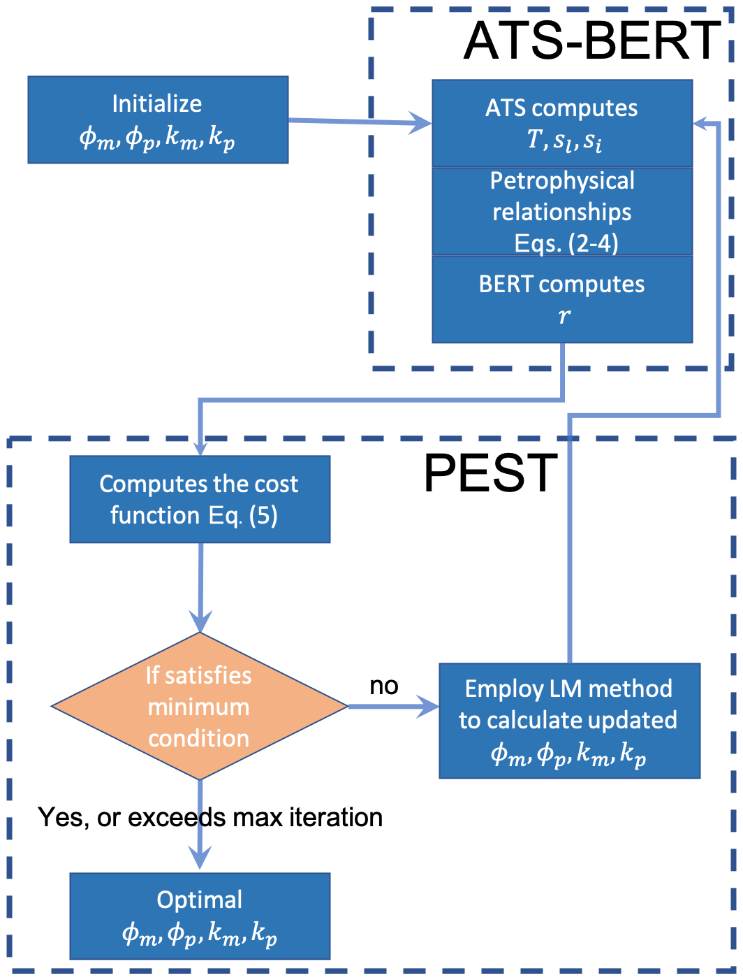
Figure 1Schematics of the parameter estimation algorithm. The algorithm starts with initial guesses on porosities and thermal conductivities for the peat and mineral layers. The coupled ATS–BERT forward model then simulates temperature (T), liquid water saturation (sl), ice saturation (si), and apparent resistivities (ρa), which are passed to the cost function. If the cost function is small enough, {ϕ,k} are considered to be the estimated parameters. If not, the values of the {ϕ,k} are updated according to the Levenberg–Marquardt (LM) minimization algorithm and passed back to the ATS–BERT model.
2.1 ATS–BERT model
To set up the synthetic model, we used digital elevation data of a transect through ice-wedge polygonal tundra at the Barrow Environmental Observatory (BEO) at Utqiaġvik, Alaska (Fig. 2). Our study includes an 11 m section covering a single polygon with an ice wedge on each side. In this study we do not explicitly assign ice properties for the ice wedges. Instead, we model bulk porosities and effective thermal conductivities that can be associated with peat and mineral layers of the entire transect.
In Fig. 2a, we present the computational mesh representing the cross section of the polygonal tundra that ATS is run on. The thickness of the peat layer corresponds to observations at the site, with a thick peat layer on the sides (troughs) and a thinner layer in the middle of the low-centered polygon. A mineral layer was assigned below the peat layer across the transect. We initially designated six synthetic direct temperature and soil moisture measurement locations within the active layer area, the maximum thaw layer from the ground surface to the top of the permafrost, similar to the sensor setup at the site (Dafflon et al., 2017). The average active layer depth is about 38 cm, as it can be seen from the ground temperatures simulated for the synthetic model run with actual meteorological data in Fig. 2b. The linear white region in Fig. 2b indicates the bottom of the active layer within the transect (0 ∘C). Then we added four more synthetic direct measurement locations below the active layer to evaluate the effect of their inclusion on PE accuracy and robustness. All observation locations are represented as stars in Fig. 2a corresponding to the locations of the collected daily averaged temperature and soil moisture time series. The temperature and soil moisture time series were recorded at depths of 5, 20, 60, and 80 cm below the surface.

Figure 2The (vertically exaggerated) 2-D transect used by the ATS model. (a) The unstructured mesh where green represents the peat layer and brown represents the mineral soil layer. Black stars represent the six sensors recording temperature and soil moisture content within the active layer. Red stars represent the four sensors recording temperature and soil moisture content below the active layer. (b) Ground temperature distribution simulated by the ATS model, corresponding to the time of maximum active layer depth. Here the depth of the active layer corresponds to the distance above the white linear feature (i.e., 0 ∘C) dividing the thawed and frozen regions of the ground. The light blue dots represent the location of the electrodes in this setup.
The setup of the ATS model followed a standard procedure described in several studies (Atchley et al., 2015; Painter et al., 2016; Jafarov et al., 2018). Typically, we set up the model in several steps: (1) initialization of the water table, (2) introduction of the energy equation to establish antecedent permafrost, and (3) spin-up of the model with simplified and actual meteorological data from the BEO station. We spun up the model until the active layer achieved cyclical equilibrium. The overall depth of the modeling domain is 50 m. We set the bottom boundary to a constant temperature of T=263.55 K and set zero heat and zero mass flux boundary conditions on the vertical sides. A seepage face was imposed at 4 cm below the surface on each side of the domain to allow drainage to the trough network to prevent water from pooling at the surface, as is typical of partially degraded polygonal ground (Liljedahl et al., 2016). We use two types of meteorological datasets as surface boundary condition drivers for the ATS model: simplified (sinusoidal air temperature, constant precipitation, and constant radiative forcing) and actual weather data from the BEO site. The actual meteorological data were collected starting on 1 January 2015 and include air temperature, rain and snow precipitation, humidity, long- and shortwave radiation, and wind speed.
We created a synthetic “truth” by designating porosities and soil grain thermal conductivities {ϕ,k} of peat and mineral soil as parameters in the forward model. The resulting temperature (T), liquid and ice saturations (sl, si), and apparent resistivities (ρa) were collected as the true state. Critical for these simulations is the calculation of the thermal conductivities of the bulk soil; calculated in ATS using Kersten numbers to interpolate between saturated frozen, saturated unfrozen, and fully dry states (Painter et al., 2016) where the thermal conductivities of each end-member state are determined by the thermal conductivity of the components (soil grains, air, water, or liquid) weighted by the relative abundance of each component in the cell (Johansen, 1977; Peters-Lidard et al., 1998; Atchley et al., 2015). Thermal conductivities of water, ice, and air are considered constant, leaving soil grain thermal conductivity as the remaining parameter to be estimated. The equation to calculate saturated, frozen thermal conductivity (κsat,f) has the following form:
where κsat,uf, κi, κw are thermal conductivities for saturated unfrozen, ice, and liquid water, respectively; and ϕ is porosity.
The freezing characteristic curve is thermodynamically derived using a Clapeyron relation and the unfrozen water retention curve, as described in Painter and Karra (2014) and Painter et al. (2016). In Fig. 3 we present liquid and ice saturations for one realization of the model for winter (January) and summer (August) times of the year. The ice saturation is high below the active layer all year long and lowest within the active layer in the summer. The peat layer holds more water; therefore, ice concentration is higher than in the mineral layer in the winter. The liquid saturation plot shows that, by the end of the summer, the peat layer is drier than the mineral layer.
We sequentially couple the ATS and BERT numerical models via petrophysical relationships used by Tran et al. (2017) and based on Archie (1942) and Minsley et al. (2015). In that approach, the electrical resistivity (ρ) is determined as a function of soil characteristics, temperature, porosity, liquid water saturation, fluid conductivity, and ice content:
where σw is the fluid electrical conductivity, σs is soil/sediment electrical conduction, n is a saturation index, d is a cementation index, and c is a temperature compensation factor accounting for deviations from T=25 ∘C.
The ice content is linked to water content through the liquid water saturation and to σw, which is influenced by the concentration of Na+ and Cl− ions and the ice–liquid fraction. Here σw has the following form:
where Fc is Faraday's constant, βi and zi are the ionic mobility and valence respectively, Ci is the concentration of the ith ion, and α is the factor influencing how the liquid water salinity increases when the fractions of liquid in ice–liquid water decrease. is defined as
Both sl and si are simulated by ATS. Note that ϕ in Eq. (2) is an estimated parameter (see Fig. 1). In this study we assume that the n, d, σs, α, Fc, , , , and parameters used in Eqs. (2) and (3) are known (see Tran et al., 2017) and focus on the robustness of the PE algorithm in estimating porosity and thermal conductivity.
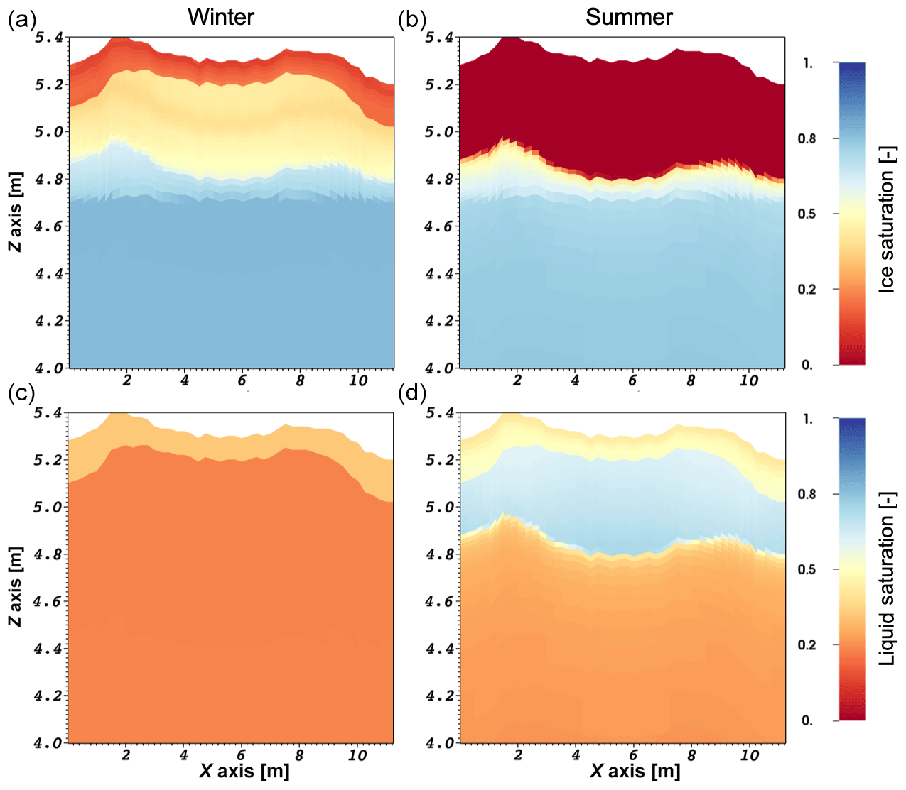
Figure 3The 2-D transects of daily snapshots simulated by the ATS model. The rows from top to bottom correspond to ice saturation (a, b) and liquid saturation (c, d). The columns from left to right correspond to a day in the middle of the winter and the day of maximum active layer depth in summer.
The 2-D resistivity data inferred from ATS simulations and petrophysical relationships get passed to BERT, which simulates resistances that are then converted to the apparent resistivities (ρa). The ρa values correspond to an acquisition along an 11 m long transect using a 0.5 m electrode spacing and a Schlumberger configuration with a total of 138 measurements (see Fig. 2b). This configuration implies that the measurements are mostly sensitive to the electrical resistivity in the top few meters.
Since BERT and ATS operate on different unstructured meshes, we wrote a function that interpolates the values between the two meshes. Note that the ATS mesh is 50 m deep. We calculate ρ by using corresponding outputs from the ATS model and the petrophysical relationships, and we then interpolated these values on a mesh defined in BERT and adapted to the acquisition geometry. BERT's mesh consists of a finely resolved mesh (11 m wide by 4.5 m deep) embedded within a coarser outer mesh that is about 120 m wide and 85 m deep. We link hydrological variables with electrical resistivities in the fine mesh. The coarse mesh is used to reduce the effect of boundaries. It extends until the change in the electrical resistivity between two neighboring cells is negligible.
2.2 Parameter estimation using PEST
To test if the known soil properties can be recovered by the PE approach, we start with randomly selected initial parameter guesses. We use a Latin hypercube sampling method to generate random initial guesses of porosity and thermal conductivities around the synthetic truth (McKay et al., 1979). Each parameter combination includes four parameters: porosity and thermal conductivity for peat and mineral soil layers. These parameters were chosen due to their strong controls on both hydrologic and thermal states (Atchley et al., 2015; Nicolsky et al., 2009). The rest of the hydrothermal properties are kept fixed.
The inverse approach involves the minimization of a cost function expressed as the sum of squared differences between simulated values and synthetic measurements using the Levenberg–Marquardt (LM) algorithm (Levenberg, 1944; Marquardt 1963) implemented in the PEST software package (Doherty, 2001), which was used to handle all parameter estimation runs.
To estimate soil porosities and thermal conductivities, we minimize the cost function (J), which includes calculated and synthetic T, sl, and ρa in the following form:
where subscripts c and s correspond to calculated and synthetic states of the system; and wT, ws, and are the corresponding weights for the temperature, saturation, and apparent resistivity residuals. nsens is the number of sensors, ndays is the number of days over which we collected the data, nsnap is the number of ρa snapshots, and nmeas is the number of ρa measurements during one snapshot. Tc and are time series from multiple sensors collected daily from the beginning of June until the end of September. ρa represents the apparent resistivity data snapshots taken at a certain day. The number of apparent resistivity snapshots depends on the particular case, varying from one to eight snapshots per year. The one-snapshot case corresponds to only one snapshot in the month of August, while the eight-snapshot case corresponds to a snapshot taken once per month from January until September. In addition, we tested the case where we collected eight daily ρa snapshots. This was done to compare how different time spacing would affect the estimated properties.
The weights were chosen in order to scale the contribution of each type of residual so that contributions to the cost function are evenly distributed across temperature, saturation, and apparent resistivity residuals. For example, saturation residuals are on the order of a few tenths, while apparent resistivity residuals can be tens of ohmmeters. The weights were selected based on evaluating the individual contributions to the cost function for each measurement type on an ensemble of simulations spanning the parameter ranges. The apparent resistivity residual weight () was set to one. The temperature and saturation residual weights (wT and ws) were then modified so that each measurement type component in the cost function had roughly equivalent magnitude over most of the parameter space. This resulted in weights of , , and .
If the cost function satisfies a minimum criterion or the maximum allowed number of iterations, which we chose to be equal to 25, is reached, the PE terminates. The porosities and thermal conductivities corresponding to the minimum of the cost function, i.e., the parameters associated with the best fit between simulated and synthetic values, are considered the estimated parameter values as
Here {ϕ,k} are the estimated porosities and thermal conductivities for peat and mineral soil.
Based on sensitivity analyses using simplified meteorological data, the cost function response surface was smooth and convex over the parameter ranges of interest. Therefore, we chose the LM approach because of its robust gradient-based optimization scheme that takes advantage of smooth convex response surfaces to quickly converge to minima.
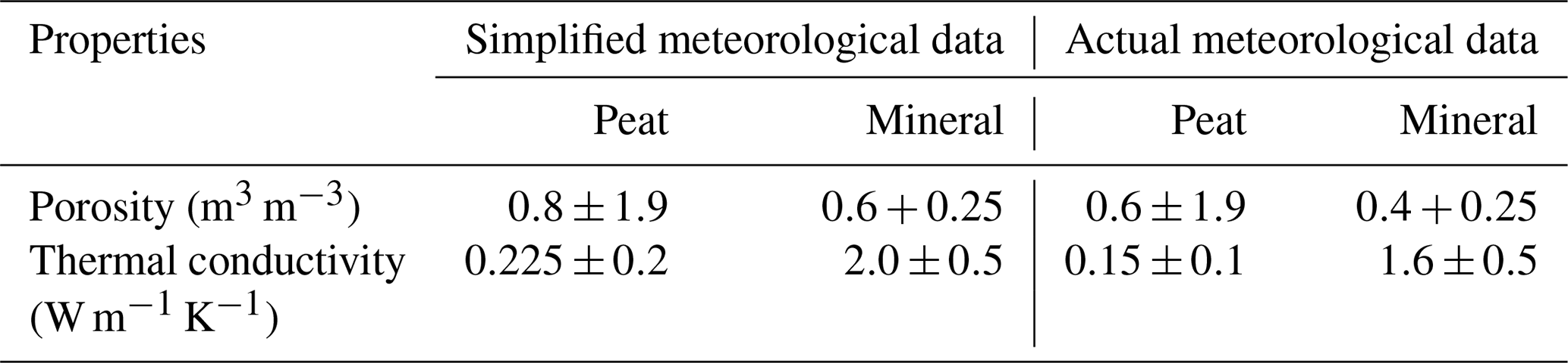
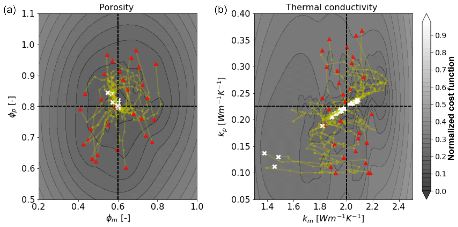
Figure 4Estimated properties from 30 inversions of the (S)3T3sl1ρa case, where the “true” values are shown as a cross section of two dashed lines for the bulk porosities and effective thermal conductivities for peat and mineral soil layers. Yellow lines correspond to the paths taken by the LM algorithm. The white dots correspond to the estimated values. (a) Projection of the cost function with respect to porosities of the peat and mineral layer. (b) Projection of the cost function with respect to thermal conductivities of the peat and mineral layer. The color bar represents the cost function normalized by its maximum logarithmic value.
2.3 Experiments
To build an understanding of the inverse framework, we start with a simple setup and then gradually add more complexity. First, we use simplified meteorological data where we assume that air temperatures change according to a sinusoidal function and all other terms are constants. Initially we start with three temperature and moisture content measurement locations within the peat layer (refer to Fig. 2a) and one ERT data snapshot. Then we increase the number of ERT data snapshots up to eight by adding snapshots once per month from January until August. Each ERT data snapshot calculated by BERT uses the set of daily averaged T and sl simulated by ATS and petrophysical relations (Eqs. 2 and 3) which are varying over time. Then we increase the number of sensors to six and add noise to the simulated data. Introduction of noise allows us to evaluate the effect of measurement uncertainties that will be present in the actual application of the PE method. We added different levels of Gaussian noise to the synthetic measurements of T, sl, and ρa in the following way: 1 % to T, 5 % to sl, and 10 % to ρa. These levels of noise for the different types of measurements are based on published literature and our own experience (Wang et al., 2018; Dafflon et al., 2017). After that we substitute simplified meteorological data with actual data from the BEO site to evaluate our PE method under realistic ground surface boundary conditions. In this case we evaluate how much and what kind of data we need to robustly recover subsurface porosities and thermal conductivities. To do this we test the inclusion of individual types of measurements in the cost function (Eq. 3) as well as all possible combinations of measurement types. We used different soil property ranges for the simplified and actual meteorological data PE runs which are summarized in Table 1. This was done to ensure that PE is able to recover different sets of parameters and to test the consistency and effectiveness of the PE method. Finally, we compared the difference between estimated parameters for eight ERT data snapshots collected once a month versus once a day for 8 d. The notation and a description of each run for simplified and actual meteorological data are summarized in Table 2.
Table 2Description of all PE cases used in this study. The numbers before T and sl correspond to the number of sensors used. The number before ρa corresponds to the number of apparent resistivity snapshots used. n stands for noise added to the synthetic measurements. (S) corresponds to runs driven by simplified meteorological data. (s) represents daily ρa snapshots.
3.1 Simplified meteorological data
To evaluate the PE method performance driven by simplified meteorological data, we ran PE experiments using 30 different random combinations of porosity and thermal conductivity values as the initial starting point. We used 30 PE samples of {ϕ,k} starting points in the first experiment ((S)3T3sl1ρa) to illustrate the overall performance of the parameter estimation using a large number of samples. After that, we did only five PE runs for the simplified meteorological data and 10 for all other runs with actual meteorological data. For all figures after Fig. 4, for consistency and clarity, we show results for only five PE runs per case. It is important to note that the number of samples that one needs to run to ensure the robust convergence of the estimated parameters depends on the specifics of the corresponding case (i.e., experiment-specific). If most of the LM runs converge to the same set of parameters and have low cost function values, then that set of runs most likely corresponds to the actual {ϕ,k}. In Fig. 4, the red triangles represent initial guesses (parameter combinations), and the synthetic truth is indicated by the intersection of the two dotted lines. Yellow lines connecting red triangles with white crosses represent the path that the LM algorithm has taken from the initial guess to the estimated parameter combination (white crosses, Fig. 4). The yellow dots along the yellow lines indicate the location at each LM iteration.
Figure 4 indicates that the method is able to recover porosities more robustly than thermal conductivities, i.e., estimated porosities are similar to their true state. According to the liquid saturation plot in Fig. 3, liquid saturation of the mineral layer is quite dynamic and more saturated in comparison to the peat layer. Nevertheless, thermal conductivity of the mineral layer (km) corresponds to the highest mismatch. Three out of 30 inversions corresponding to km end up close to 1.4 W m−1 K−1 (the true value is 2 W m−1 K−1), suggesting those values do not correspond to the truth, since most of the estimated values (27 cases) are concentrated around the intersection of the dotted lines. The response surface for the corresponding cost function (Eq. 5) lies hereby in a flat, low-gradient region. The projections of the cost function response surfaces corresponding to porosities (Fig. 4a) have a better defined minimum, as opposed to projections of the cost function response surfaces corresponding to thermal conductivities (Fig. 4b), indicating the nonuniqueness of the estimated parameters. For this experiment, we used time series of T and sl only from the first three near-surface sensors (Fig. 2a). All of these three sensors are located in the peat layer, suggesting that using just near-surface sensors only from one upper layer might not be enough to recover the deeper layer thermal conductivity.
To illustrate the effect of noise on the robustness of the estimated parameters we used cases with six near-surface sensors (6T and 6sl) and a varying number of ERT snapshots driven with simplified meteorological data. Similarly to the (S)3T3sl1ρa case, (S)6T6sl1ρa shows good convergence for porosities and poor convergence for thermal conductivities with an averaged error of 0.1 W m−1 K−1 (Fig. 5a, b). Adding noise to the (S)6T6sl1ρa+n case slightly worsens the estimated porosity values and significantly worsens km with root-mean-squared error (RMSE) rising from 10 % to more than 50 % (Fig. 5c, d). Figure 5e and f show that increasing the number of ERT snapshots from one to eight per year (i.e., collected once per month from January until September) improves km estimates, allowing better convergence for four out of five samples to the synthetic truth. If we compare all three cases in Fig. 5 on how well they are able to estimate km, it is clear from Fig. 5d that for the case (S)6T6sl1ρa+n none of the km's were correctly estimated, whereas significantly improved km values were found by increasing the number of monthly ERT snapshots (Fig. 5f). Moreover, all except one estimated value showed a better match with its true value than the (S)6T6sl1ρa case without any added noise.
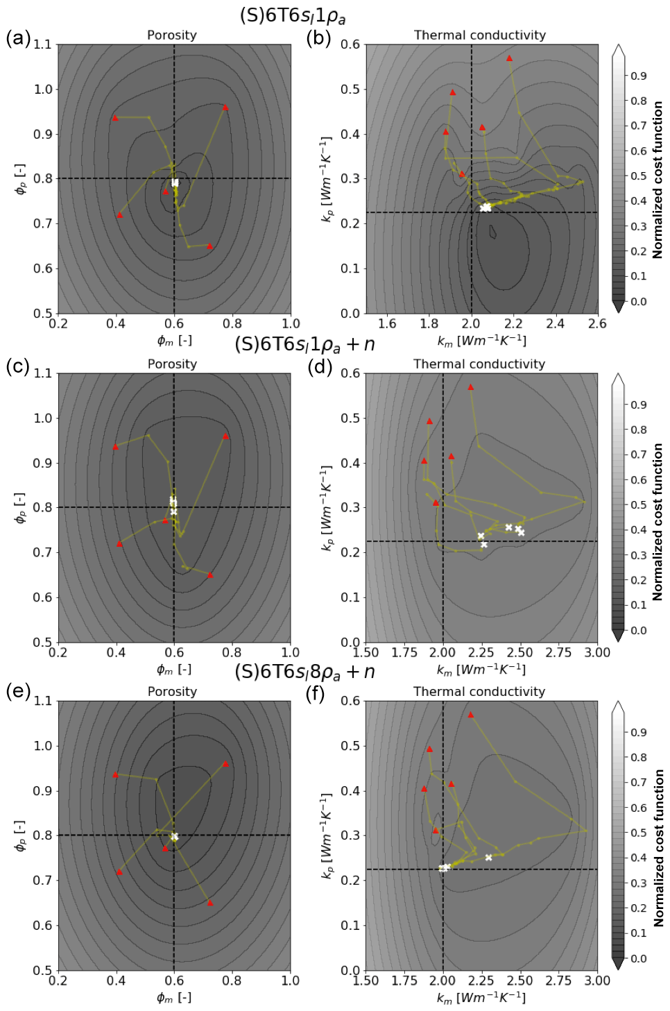
Figure 5Estimated properties from five inversions of the three different cases, where the true values are shown as a cross section of the two dashed lines for the bulk porosities and effective thermal conductivities for peat and mineral soil layers. Yellow lines correspond to the paths taken by the LM algorithm. The white dots correspond to the estimated values. The rows from top to bottom correspond to cases (S)6T6sl1ρa (a, b), (S)6T6sl1ρa+n (c, d), and (S)6T6sl8ρa+n (e, f) respectively. The columns from left to right correspond to the projection of the cost function with respect to porosities and thermal conductivities. The color bar represents the cost function normalized by its maximum logarithmic value.
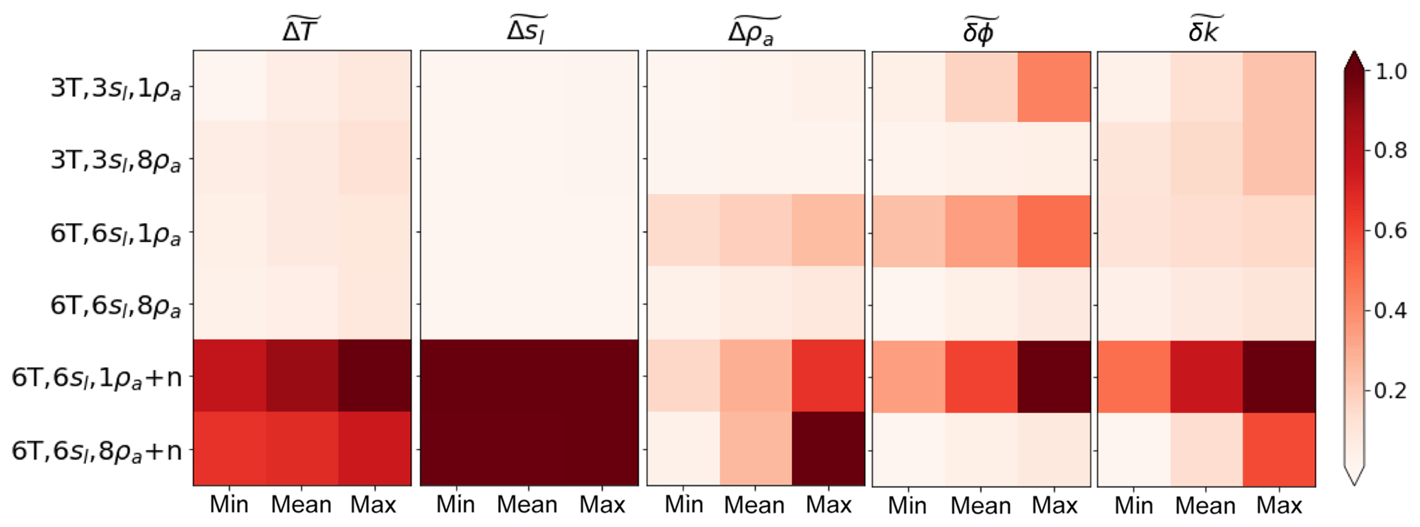
Figure 6Five matrix tables presenting fitness metrics between synthetic model values and values obtained by the parameter estimation method using simplified meteorological data. Matrix tables from left to right correspond to the normalized root-mean-squared errors for temperatures, liquid water saturations, and apparent resistivities as well as to the normalized Euclidian distances between synthetic (true) and estimated values of porosities and thermal conductivities. Each matrix value was normalized by dividing it by the matrix maximum value. The normalized values are indicated by tildes.
In Fig. 6, we summarize results of the five PE runs for each of the first six cases corresponding to simplified meteorological data listed in Table 2. The first three matrix tables correspond to the normalized RMSE values for each measurement type (ΔT, Δsl, and Δρa). The last two matrix tables correspond to the normalized Euclidian distances between the synthetic truth and estimated parameter values of δϕ and δk. We normalized the values in each matrix by dividing by the maximum value from the corresponding matrix. The normalized values are marked with tildes and range from 0 to 1, where values closer to 0 correspond to a better match and values closer to 1 correspond to a worse match. As shown above, the method is able to accurately estimate both peat and mineral soil porosities as well as peat layer thermal conductivity (kp), but it cannot always accurately estimate km. There is not much difference between cases (S)3T3sl1ρa and (S)6T6sl1ρa except for a slight improvement in km, suggesting that the small vertical distance (10 cm) between sensors 1 and 4, 2 and 5, and 3 and 6 could limit the recorded data variability, leading to difficulties in the estimation of the km parameter. Since all six sensors lie within the active layer, we added additional sensors below the active layer in the later experiments (red stars in Fig. 2a). The ϕ and k matrix tables show that increasing the number of monthly ERT snapshots consistently improves the estimates of ϕ and k. This suggests that increasing the number of monthly ERT snapshots can lead to improved convexity of the cost function (Eq. 5).
3.2 Meteorological data from the Utqiaġvik (Barrow) site 2015
After testing the PE method for the simplified meteorological data, we applied measured meteorological data from the BEO site for the year 2015. To better understand the importance of each measurement type and their combinations within the developed PE algorithm, we tested all of the scenarios corresponding to the “actual meteorological data” column from Table 2. The results of these runs are summarized in the colored matrix tables in Fig. 7. Since there are more than twice the number of actual meteorological cases than simplified meteorological cases, it is difficult to analyze all matrix tables at once.
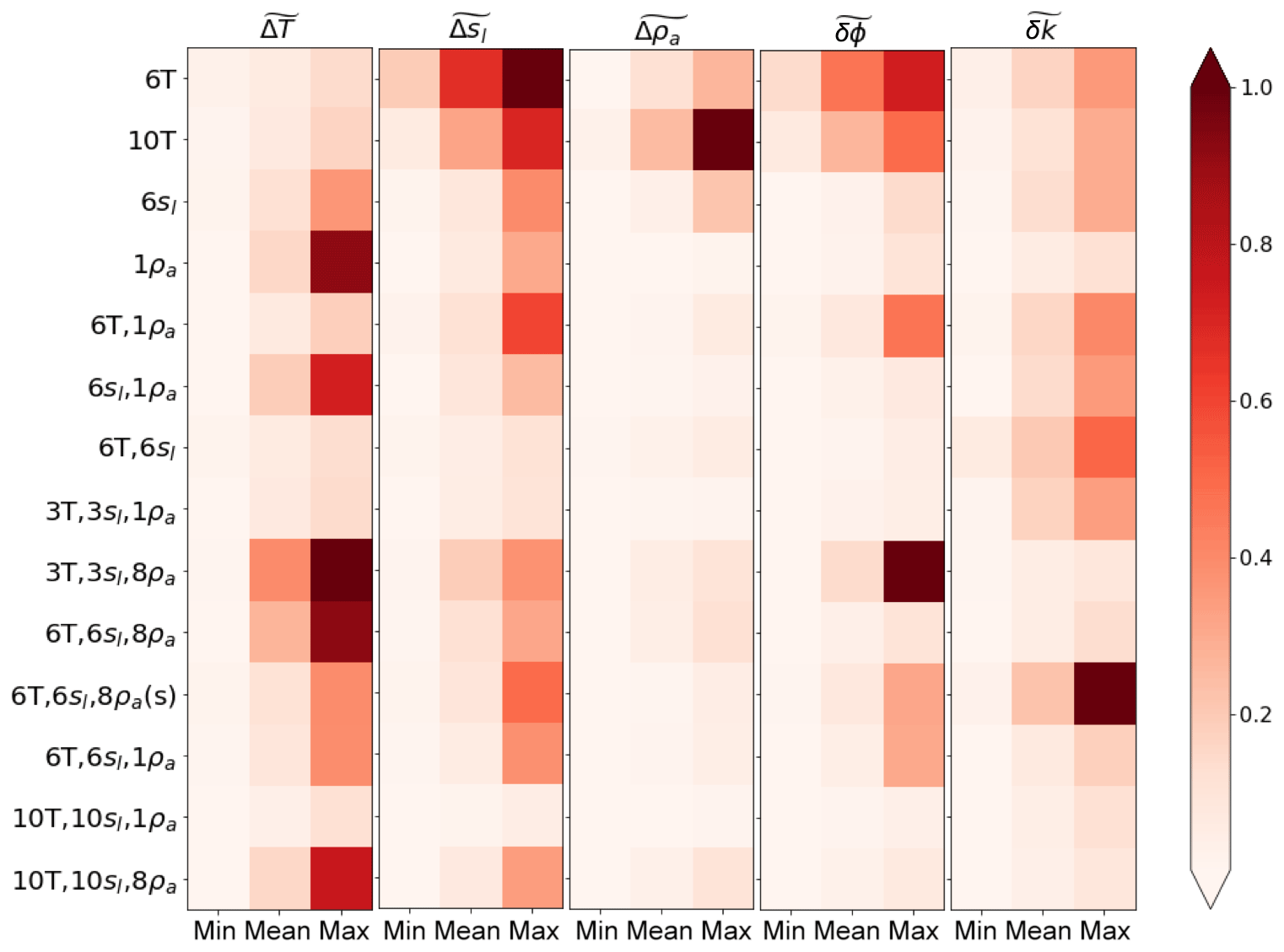
Figure 7Five matrix tables presenting fitness metrics between synthetic model values and values obtained by the parameter estimation method using meteorological data from the year 2015 from the BEO site in Alaska. Matrix tables from left to right correspond to the normalized root-mean-squared errors for temperatures, liquid water saturations, and apparent resistivities as well as to the normalized Euclidian distances between synthetic (true) and estimated values of porosities and thermal conductivities. Each matrix value was normalized by dividing it by the matrix maximum value. The normalized values are indicated by tildes.
To compare the match between all estimated and observational values within a single plot we calculated Euclidean norms for each case independently:
The index i indicates the case number (see Table 2). Then we applied k-means clustering analysis to identify groups of cases with a similar match between data and estimated parameters. We divided all cases into four classes shown in Fig. 8. Class I indicates the best cases that provide an accurate parameter estimation as well as accurate matches with the synthetic true measurements. Class II includes the cases that have accurate parameter estimates and less accurate matches with the measurements. Class III indicates all cases that have less accurate parameter estimates but accurate matches with the measurements. Finally, class IV includes the cases that showed the worst performance in terms of parameter estimates and the worst matches with the measurements. We summarized the results from Fig. 8 in Table 3.
Class I (see Table 3) suggests that sensors located below the active layer as well as increasing the number of sensors lead to more accurate parameter estimation. In contrast, case no. 4 (corresponding to the one ERT snapshot, 1ρa) suggests that already one ERT data snapshot could be enough for parameter estimation, while class II indicates that in general an increase in the numbers of monthly ERT snapshots is important for more accurate PE. However, increasing the number of monthly ERT snapshots leads to a less accurate match with measurements. These results are consistent with the results for simplified meteorological data with added noise (Fig. 5).
Class III includes six cases suggesting that if we have only soil moisture data available for PE, then we should expect less accurate soil property estimates. The last element in this class suggests that taking daily ERT snapshots improves the apparent resistivity match (Fig. 7, resistivity table) but does not improve {ϕ,k} estimates, where monthly ERT snapshots improve thermal conductivity convergence.
Class IV once again clearly indicates that measurements obtained below the active layer provide more accurate parameter estimates; however, they do not improve matches to measurements. This is mainly due to significant mismatch with ρa, which can be seen from the matrix table in Fig. 8. At the actual site, the depth to the mineral soil can be deeper than 20 cm; not having sensors lower than 20 cm therefore limits the amount of data that can help to improve the convexity of the cost function in our case.
Table 3K-means analysis of the accuracy for each of the 13 cases.
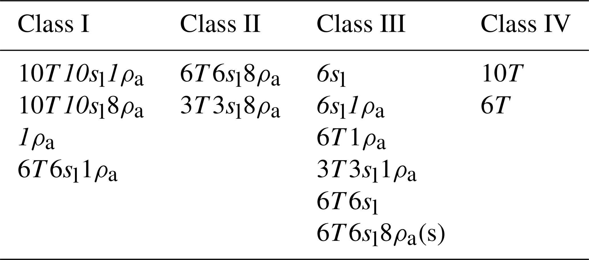
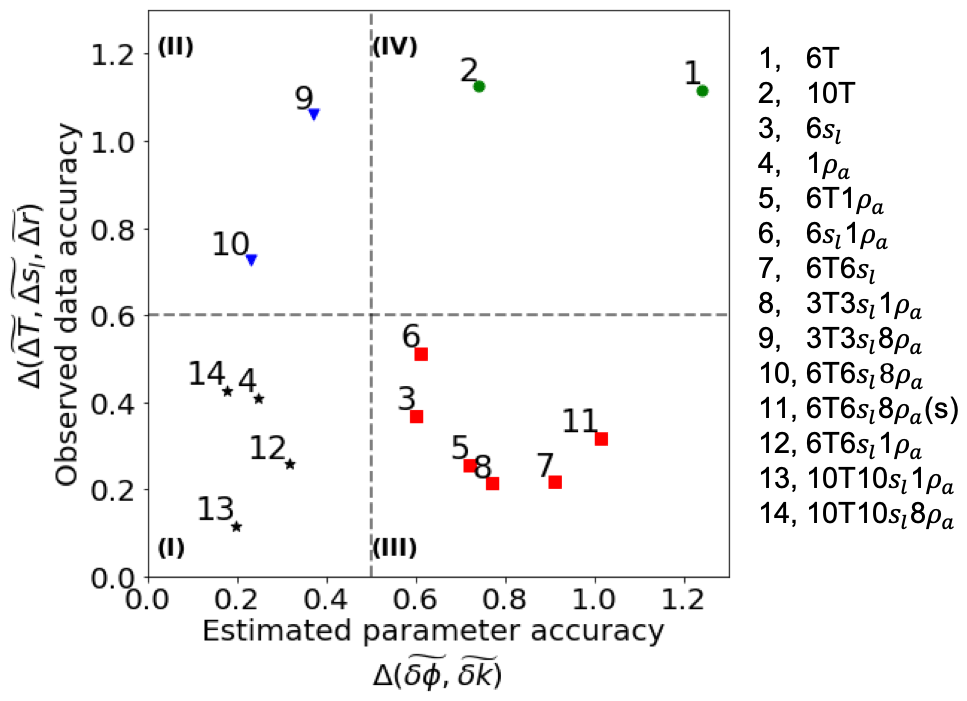
Figure 8A k-means clustering analysis applied to the Euclidean norms of the normalized mean differences of estimated soil properties and the corresponding fit between calculated and observed values. Each color and marker represent a certain class as a result of the k-means clustering analysis.
From Fig. 8 and Table 3 we know that the 6T case has the worst performance in terms of matching {ϕ,k}. Similar to the experiments with simplified meteorological data, the main difficulty for experiments with actual meteorological data is estimating thermal conductivity. The last matrix table () in Fig. 7 shows that 6T6sl8ρa(s) has the highest maximum and mean mismatch in thermal conductivity estimates. However, since ϕ estimates are a better match with their corresponding true values, the case 6T6sl8ρa(s) falls into class III in Fig. 8, as opposed to case 6T, which falls into class IV. The highest mismatch in thermal conductivity values for the 6T6sl8ρa(s) case suggests that collecting daily ERT snapshots improves the ρa match (Fig. 7, matrix table) but does not improve estimated parameters, where monthly ERT snapshots improve thermal conductivity estimation.
To illustrate this, we plot values of estimated parameters and the corresponding response surfaces of the cost function for cases 10T10sl8ρa and 6T6sl8ρa(s) in Fig. 9. The PE method was able to match four out of five estimates almost perfectly and missed the kp for the 10T10sl8ρa case. The corresponding cost function has a visible minimum and clear convexity. In contrast to this, the 6T6sl8ρa(s) case completely missed two estimates by converging on values outside the boundaries, and three other estimates do not converge to the desired cross section as well. The contour lines suggest that the corresponding response surfaces of the cost function do not have a well-defined global minimum.
The existence of multiple minima is common in inverse modeling and can lead to a false convergence of the PE algorithm to physically nonrealistic subsurface parameters (Nicolsky et al., 2007). This is one of the main reasons for using multiple initial guesses. If most of the inversions converge to a similar set of parameter estimates with the lowest cost function value, then that set of values is most likely the global minimum. Testing the PE algorithm using multiple starting points is a commonly used approach in evaluating the robustness of an inverse model (e.g., Hansen, 1998).
A potential strategy to improve the developed PE algorithms is to reduce the specified convergence tolerance value (i.e., minimum condition; see Fig. 1) or increase the allowable number of iterations. However, this could lead to a significant increase in computational effort. In addition, PEST provides multiple additional settings of inversion parameters to achieve a better convergence. Parameter regularization is one of them. Regularization techniques have been widely used in solving ill-posed inverse problems (Vogel, 2002). The overall idea is to constrain the objective function by imposing additional priors on the estimated model parameters. We recognize that including parameter regularization into the cost function may improve the robustness of our method. However, inclusion of the regularization would require an extensive exploration of the multiple regularization methods and values that could be applied to it, which is beyond the scope of this paper. Here we illustrate that without using regularization it is possible to achieve reasonable results by using the simple weighted cost function.
The good performance of the case with only one ERT snapshot (1ρa) could be misleading due to the design of this numerical experiment; i.e., we are using a synthetic truth produced by the same model used in the inversion, which improves the convexity of the cost function and leads to a well-constrained unique minimum. However, in reality, the collection of additional information, such as organic layer thickness and temperature data, is extremely important and is required for model calibration (Jafarov et al., 2012; Atchley et al., 2015). In addition, real ERT surveys can be perturbed by noise, and their interpretation may require site-specific petrophysical relationships as opposed to the general petrophysical relationships used in this study. Therefore, we do not suggest an inversion based on one ERT snapshot without any additional data.
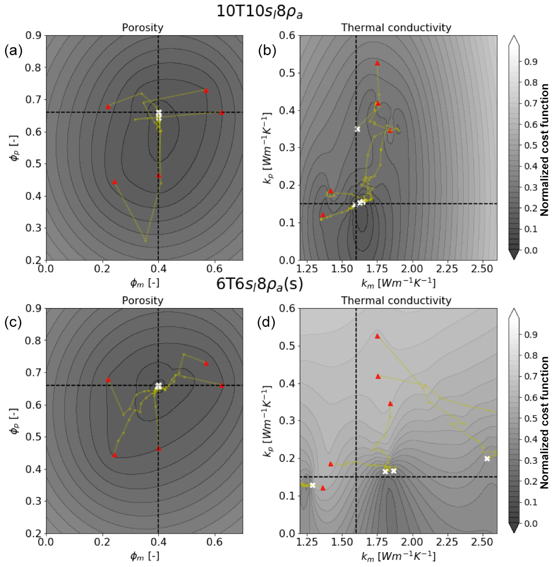
Figure 9Estimated properties from five inversions of the two different cases: 10T10sl8ρa (a) and 6T6sl8ρa(s) (b). The true values are shown as a cross section of the two dashed lines for the bulk porosities and effective thermal conductivities for peat and mineral soil layers. Yellow lines correspond to the paths taken by the LM algorithm. The white dots correspond to the estimated values. The columns from left to right correspond to the projection of the cost function with respect to porosities and thermal conductivities. The color bar represents the cost function normalized by its maximum logarithmic value.
The 6T6sl8ρa(s) case, where all runs converge to different values of km, indicates that using certain combinations of datasets does not allow the inverse approach to properly recover km. It is likely that 6T6sl8ρa(s) does not capture much variability in soil temperatures and soil moisture, and therefore ERT snapshots do not have much variability as well. Once the cost function converges for one of the ERT snapshots, it immediately converges on the other daily snapshots due to their similarity. In fact, although 6T6sl8ρa(s) has a good accuracy with observations (see the matrix table in Fig. 7), it is unable to recover the value of km.
We have shown that, even in the ideal situation where we either generate observational data or use simplified meteorological data, we cannot always fit modeling results to observations. In reality, noise (e.g., the sensor's measuring resolution) influences the collected data. To investigate the impact of measurement noise, we introduced multiple levels of noise to the simplified meteorological data. The resulting PE showed that dealing with noisy data could be challenging (Fig. 5). However, our results showed that adding ERT snapshots taken monthly into the cost function improves the overall PE accuracy.
The distance between sensors could be another source of uncertainty in the PE. As pointed out by Nicolsky et al. (2009), it is important to make sure that a vertical difference between adjacent measurements does not introduce additional noise that can mislead the minimization algorithm without providing new information. If sensors are close to each other, measurements might be the same or within the noise variability. In our setup the vertical distance between the first two rows of sensors is about 15 cm. This could lead to small temperature variability between sensors. Indeed, providing greater vertical distance between sensors improved the PE accuracy. Case no. 12 (6T6sl1ρa) clearly illustrates this point – that by increasing the vertical distance between sensors we can improve estimated parameter accuracy.
Combining hydrothermal observations from multiple depths with monthly ERT measurements resulted in an improvement of the shape of the cost function and led to better defined minima (Fig. 9). Increasing the number of the monthly ERT snapshots improved the accuracy of the estimated parameters. In addition, we showed that having sensors below the active layer combined with ERT snapshots shows the best accuracies both in terms of estimating parameters and matching observations.
The overarching goal of this study was to develop and validate a parameter estimation algorithm using a synthetic setup and a 2-D coupled thermal–hydrological–geophysical model based on a polygonal tundra site within the Barrow Environmental Observatory. Combining hydrothermal observations from multiple depths with monthly ERT measurements resulted in an improved shape of the cost function and led to better defined minima and improved accuracy of the estimated parameters. This was presented in fitness matrices for six cases using simplified meteorological data. Similar conclusions were found for inversion runs with actual meteorological data. It is important to note that it was not only the number of ERT data snapshots that improved the robustness of the PE method but rather the time frequency of the ERT data snapshots, i.e., monthly vs. daily snapshots. In addition, collecting data from several soil layers might improve the thermal conductivity estimates for the corresponding soil layer. Our experiments show that robust PE can be achieved not just by adding more sensors into the ground and increasing the number of ERT snapshots but also by optimally distributing those sensors within the transect (e.g., the 6T6sl1ρa case). Overall, the inversion runs that we investigated consistently indicated that collecting data from multiple soils layers, providing enough vertical separation between sensors, and collecting temporally diverse ERT data should lead to robust parameter estimation. The exception from this conclusion is the case 1ρa, which showed robust parameter estimation due to specifics of the model setup. As discussed above, estimating porosities and thermal conductivities based on one ERT snapshot would not be possible without additional information on the subsurface properties.
This work developed and demonstrated the feasibility of a PE algorithm that can be used to better inform large-scale land system model subsurface parameterization. Here we demonstrated the proof of concept of the PE method. Further improvements such as the introduction of a PE regularization parameter into the cost function and leveraging additional PEST capabilities could improve method robustness. Finally, the PE method must still be tested using measured thermal–hydrological–geophysical data from the BEO site.
Forcing data used in these simulations can be downloaded from https://github.com/amanzi/ats-testsuite-arctic/tree/master/testing/Data/ (last access: 3 January 2020).
Numerical simulations were performed by EEJ and DRH with guidance from BD and ETC. BD and APT provided advice and guidance with ERT model and related coupling. EEJ and DRH contributed to the overall design of the research with guidance from CJW. ALA assisted with the writing process and references. YL provided expert knowledge on inverse modeling.
The authors declare that they have no conflict of interest.
The authors thank Vladimir Romanovsky, Joel Rowland, and Anna Liljedahl for preparing meteorological data used in this study.
This research has been supported by the Office of Biological and Environmental Research in the DOE Office of Science (NGEE Arctic).
This paper was edited by Christian Hauck and reviewed by Christian Hauck and two anonymous referees.
Abolt, C. J., Young, M. H., Atchley, A. L., and Harp, D. R.: Microtopographic control on the ground thermal regime in ice wedge polygons, The Cryosphere, 12, 1957–1968, https://doi.org/10.5194/tc-12-1957-2018, 2018.
Alifanov, O., Artyukhin, E., and Rumyantsev, S.: Extreme Methods for Solving Ill-posed Problems with Application to Inverse Heat Transfer Problems. Begell House, New York, 1996.
Archie, G. E.: The electrical resistivity log as an aid in determining some reservoir characteristics, Society of Petroleum Engineers, T. AIME, 146, 54–62, 1942.
Atchley, A. L., Painter, S. L., Harp, D. R., Coon, E. T., Wilson, C. J., Liljedahl, A. K., and Romanovsky, V. E.: Using field observations to inform thermal hydrology models of permafrost dynamics with ATS (v0.83), Geosci. Model Dev., 8, 2701–2722, https://doi.org/10.5194/gmd-8-2701-2015, 2015.
Beck, J., Clair, C. S., and Blackwell, B.: Inverse Heat Conduction: Ill-Posed Problems, Wiley, New York, 1985.
Biskaborn, B. K., Smith, S. L., and Noetzli, J.: Permafrost is warming at a global scale, Nat. Commun., 10, 264, https://doi.org/10.1038/s41467-018-08240-4, 2019.
Boike, J. and Roth, K.: Time domain reflectometry as a field method for measuring water content and soil water electrical conductivity at a continuous permafrost site, Permafrost Periglac., 8, 359–370, 1997.
Dafflon, B., Oktem, R., Peterson, J., Ulrich, C., Tran, A. P., Romanovsky, V., and Hubbard, S.: Coincident above and below-ground autonomous monitoring strategy: Development and use to monitor Arctic ecosystem freeze thaw dynamics, J. Geophys. Res.-Biogeo., 122, 1321–1342, https://doi.org/10.1002/2016JG003724, 2017.
Doherty, J.: PEST-ASP user's manual, Watermark Numerical Computing, Brisbane, Australia, 2001.
Hansen, P. C.: Rank-Deficient and Discrete Ill-Posed Problems: Numerical Aspects of Linear Inversion, Society for Industrial and Applied Mathematics, 263 pp., https://doi.org/10.1137/1.9780898719697, 1998.
Harp, D. R., Atchley, A. L., Painter, S. L., Coon, E. T., Wilson, C. J., Romanovsky, V. E., and Rowland, J. C.: Effect of soil property uncertainties on permafrost thaw projections: a calibration-constrained analysis, The Cryosphere, 10, 341–358, https://doi.org/10.5194/tc-10-341-2016, 2016.
Hjort, J., Karjalainen, O., Aalto, J., Westermann, S., Romanovsky, V. E., Nelson, F. E. Etzelmüller, B., and Luoto, M.: Degrading permafrost puts Arctic infrastructure at risk by mid-century, Nat. Commun., 9, 5147, https://doi.org/10.1038/s41467-018-07557-4, 2018.
Jafarov, E. E., Marchenko, S. S., and Romanovsky, V. E.: Numerical modeling of permafrost dynamics in Alaska using a high spatial resolution dataset, The Cryosphere, 6, 613–624, https://doi.org/10.5194/tc-6-613-2012, 2012.
Jafarov, E. E., Coon E. T., Harp, D. R., Wilson, C. J., Painter, S. L., Atchley, A. L., and Romanovsky, V. E.: Modeling the role of preferential snow accumulation in through talik development and hillslope groundwater flow in a transitional permafrost landscape, Environ. Res. Lett., 13, 105006, https://doi.org/10.1088/1748-9326/aadd30, 2018.
Johansen, O.: Thermal Conductivity of Soils No. CRREL-TL-637 Cold Regions Research and Engineering Lab, Hanover, NH, 1977.
Kern, J. S.: Spatial Patterns of Soil Organic Carbon in the Contiguous United States, Soil Sci. Soc. Am. J., 58, 439–455, 1994.
Koven, C. D., Riley, W. J., and Stern, A.: Analysis of permafrost thermal dynamics and response to climate change in the CMIP5 earth system models, J. Climate, 26, 1877–1900, https://doi.org/10.1175/JCLI-D-12--00228.1, 2013.
Levenberg, K.: A method for the solution of certain non-linear problems in least squares, Quart. Appl. Math., 2, 164–168, 1944.
Liljedahl, A. K., Boike, J., Daanen, R. P., Fedorov, A. N., Frost, G. V., Grosse, G., Hinzman, L. D., Iijma, Y., Jorgenson, J. C., Matveyeva, N., Necsoiu, M., Raynolds, M. K., Romanovsky, V. E., Schulla, J., Tape, K. D., Walker, D. A., Wilson, C. J., Yabuki, H., and Zona, D.: Pan-Arctic ice-wedge degradation in warming permafrost and its influence on tundra hydrology, Nat. Geosci., 9, 312–318, 2016.
Marquardt, D. W.: An algorithm for least-squares estimation of nonlinear parameters, J. Soc. Ind. Appl. Math., 11, 431–441, 1963.
McKay, M. D., Beckman, R. J., and Conover, W. J.: A Comparison of Three Methods for Selecting Values of Input Variables in the Analysis of Output from a Computer Code, American Statistical Association, 21, 239–245, https://doi.org/10.2307/1268522, 1979.
McGuire, A. D., Lawrence, D. M., Koven, C., Clein, J. S., Burke, El., Chen, G., Jafarov, E., MacDougall, A. H., Marchenko, S., Nicolsky, D., Peng, S., Rinke, A., Ciais, P., Gouttevin, I., Hayes, D. J., Ji, D., Krinner, G., Moore, J. C., Romanovsky, V., Schädel, C., Schaefer, K., Schuur, E. A. G., and Zhuang, Q.: The dependence of the evolution of carbon dynamics in the northern permafrost region on the trajectory of climate change, P. Natl. Acad. Sci. USA, 115, 3882–3887, 2018.
Minsley, B. J., Wellman, T. P., Walvoord, M. A., and Revil, A.: Sensitivity of airborne geophysical data to sublacustrine and near-surface permafrost thaw, The Cryosphere, 9, 781–794, https://doi.org/10.5194/tc-9-781-2015, 2015.
Nicolsky, D. J., Romanovsky, V. E., and Tipenko, G. S.: Using in-situ temperature measurements to estimate saturated soil thermal properties by solving a sequence of optimization problems, The Cryosphere, 1, 41–58, https://doi.org/10.5194/tc-1-41-2007, 2007.
Nicolsky, D. J., Romanovsky, V. E., and Panteleev, G. G.: Estimation of soil thermal properties using in-situ temperature measurements in the active layer and permafrost, Cold Reg. Sci. Technol., 55, 120–129, 2009.
Oleson, K. W., Lawrence, D. M., Gordon, B., Bonan, G. B., Drewniak, B., Huang, M., Koven, C. D., Levis, S., Li, F., Riley, J. W., Subin, Z. M., Swenson, S. C., and Thornton, P. E.: Technical description of version 4.5 of the Community Land Model (CLM), NCAR Technical Note NCAR/TN-503CSTR, 420 pp., https://doi.org/10.5065/D6RR1W7M, 2013.
Painter, S. L. and Karra, S.: Constitutive model for unfrozen water content in subfreezing unsaturated soils, Vadose Zone J., 13, https://doi.org/10.2136/vzj2013.04.0071, 2014.
Painter, S. L., Coon, E. T., Atchley, A. L., Berndt, M., Garimella, R., Moulton, J. D., Svyatskiy, D., and Wilson, C. J.: Integrated surface/subsurface permafrost thermal hydrology: model formulation and proof-of-concept simulations, Water Resour. Res., 52, 6062–6077, 2016.
Peters-Lidard, C. D., Blackburn, E., Liang, X., and Wood, E. F.: The effect of thermal conductivity parameterization on surface energy fluxes and temperatures, J. Atmos., 55, 1209–1224, 1998.
Rücker, C., Günther, T., and Spitzer, K.: Three-dimensional modelling and inversion of DC resistivity data incorporating topography – I. modelling, Geophys. J. Int., 166, 495–505, https://doi.org/10.1111/j.1365-246X.2006.03010.x, 2006
Schuster, P. F., Schaefer, K. M., Aiken, G. R., Antweiler, R. C., DeWild, J. F., Gryziec, J. D., Gusmeroli, A., Hugelius, G., Jafarov, E., Krabbenhoft, D. P., Liu, L., Herman-Mercer, N., Mu, C., Roth, D. A., Schaefer, T., Striegl, R. G., Wickland, K. P., and Zhang, T.: Permafrost stores globally significant amount of mercury, Geophys. Res. Lett, 45, GRL56886, https://doi.org/10.1002/2017GL075571, 2018.
Smith, M. and Tice, A.: Measurement of the unfrozen water content of soils comparison of NMR and TDR methods, CRREL Report 88-18, US Army Cold Regions Research and Engineering Lab, 16 pp., 1988.
Tran, A. P., Dafflon, B., and Hubbard, S. S.: Coupled land surface–subsurface hydrogeophysical inverse modeling to estimate soil organic carbon content and explore associated hydrological and thermal dynamics in the Arctic tundra, The Cryosphere, 11, 2089–2109, https://doi.org/10.5194/tc-11-2089-2017, 2017.
Vogel, C. R.: Computational Methods for Inverse Problems, SIAM, 183 pp., ISBN: 9780898715507, 2002.
Wang, K., Jafarov, E., Overeem, I., Romanovsky, V., Schaefer, K., Clow, G., Urban, F., Cable, W., Piper, M., Schwalm, C., Zhang, T., Kholodov, A., Sousanes, P., Loso, M., and Hill, K.: A synthesis dataset of permafrost-affected soil thermal conditions for Alaska, USA, Earth Syst. Sci. Data, 10, 2311–2328, https://doi.org/10.5194/essd-10-2311-2018, 2018.
Yoshikawa, K., Overduin, P., and Harden, J.: Moisture content measurements of moss (Sphagnum spp.) using commercial sensors, Permafrost Periglac., 15, 309–318, 2004.