the Creative Commons Attribution 4.0 License.
the Creative Commons Attribution 4.0 License.
 | 09 Apr 2019
Modelling the future evolution of glaciers in the European Alps under the EURO-CORDEX RCM ensemble
Matthias Huss
Daniel Farinotti
Glaciers in the European Alps play an important role in the hydrological cycle, act as a source for hydroelectricity and have a large touristic importance. The future evolution of these glaciers is driven by surface mass balance and ice flow processes, of which the latter is to date not included explicitly in regional glacier projections for the Alps. Here, we model the future evolution of glaciers in the European Alps with GloGEMflow, an extended version of the Global Glacier Evolution Model (GloGEM), in which both surface mass balance and ice flow are explicitly accounted for. The mass balance model is calibrated with glacier-specific geodetic mass balances and forced with high-resolution regional climate model (RCM) simulations from the EURO-CORDEX ensemble. The evolution of the total glacier volume in the coming decades is relatively similar under the various representative concentrations pathways (RCP2.6, 4.5 and 8.5), with volume losses of about 47 %–52 % in 2050 with respect to 2017. We find that under RCP2.6, the ice loss in the second part of the 21st century is relatively limited and that about one-third (36.8 % ± 11.1 %, multi-model mean ±1σ) of the present-day (2017) ice volume will still be present in 2100. Under a strong warming (RCP8.5) the future evolution of the glaciers is dictated by a substantial increase in surface melt, and glaciers are projected to largely disappear by 2100 (94.4±4.4 % volume loss vs. 2017). For a given RCP, differences in future changes are mainly determined by the driving global climate model (GCM), rather than by the RCM, and these differences are larger than those arising from various model parameters (e.g. flow parameters and cross-section parameterisation). We find that under a limited warming, the inclusion of ice dynamics reduces the projected mass loss and that this effect increases with the glacier elevation range, implying that the inclusion of ice dynamics is likely to be important for global glacier evolution projections.
- Article
(12738 KB) -
Supplement
(11957 KB) - BibTeX
- EndNote


In the coming century, glaciers are projected to lose a substantial part of their volume, maintaining their position as one of the main contributors to sea-level rise (Slangen et al., 2017; Bamber et al., 2018; Marzeion et al., 2018; Moon et al., 2018; Parkes and Marzeion, 2018). In the European Alps the retreat of glaciers will have a large impact, as glaciers play an important role in river runoff (e.g. Hanzer et al., 2018; Huss and Hock, 2018; Brunner et al., 2019), hydroelectricity production (e.g. Milner et al., 2017; Patro et al., 2018) and touristic purposes (e.g. Fischer et al., 2011; Welling et al., 2015; Stewart et al., 2016).
In order to understand how the ca. 3500 glaciers of the European Alps (Pfeffer et al., 2014) (Fig. 1a) will react to changing 21st century climatic conditions (e.g. Gobiet et al., 2014; Christidis et al., 2015; Frei et al., 2018; Stoffel and Corona, 2018), to date, models of various complexity have been used. Regional glacier evolution studies in the Alps (Zemp et al., 2006; Huss, 2012; Salzmann et al., 2012; Linsbauer et al., 2013) have focused on methods in which ice dynamics are not explicitly accounted for, and the glacier evolution is based on parameterisations. One of the first studies to estimate the future evolution of all glaciers in the European Alps was performed by Haeberli and Hoelzle (1995), who used glacier inventory data and combined this with a parameterisation scheme to predict the future evolution of the Alpine ice mass. In another study, Zemp et al. (2006) utilised a statistical calibrated equilibrium-line altitude (ELA) model to estimate future area losses. More recently, Huss (2012) modelled the future evolution of about 50 large glaciers with a retreat parameterisation and extrapolated these findings to the entire European Alps. The future evolution of glaciers in the European Alps was also modelled as a part of global studies, relying on methods that parameterise glacier changes through volume–area–length scaling (Marzeion et al., 2012; Radić et al., 2014) and methods in which geometry changes are imposed based on observed changes (Huss and Hock, 2015). These regional and global studies generally suggest a glacier volume loss of about 65 %–80 % between the early 21st century and 2100 under a moderate warming (RCP2.6 and RCP4.5) and an almost complete disappearance of glaciers under warmer conditions (RCP8.5).
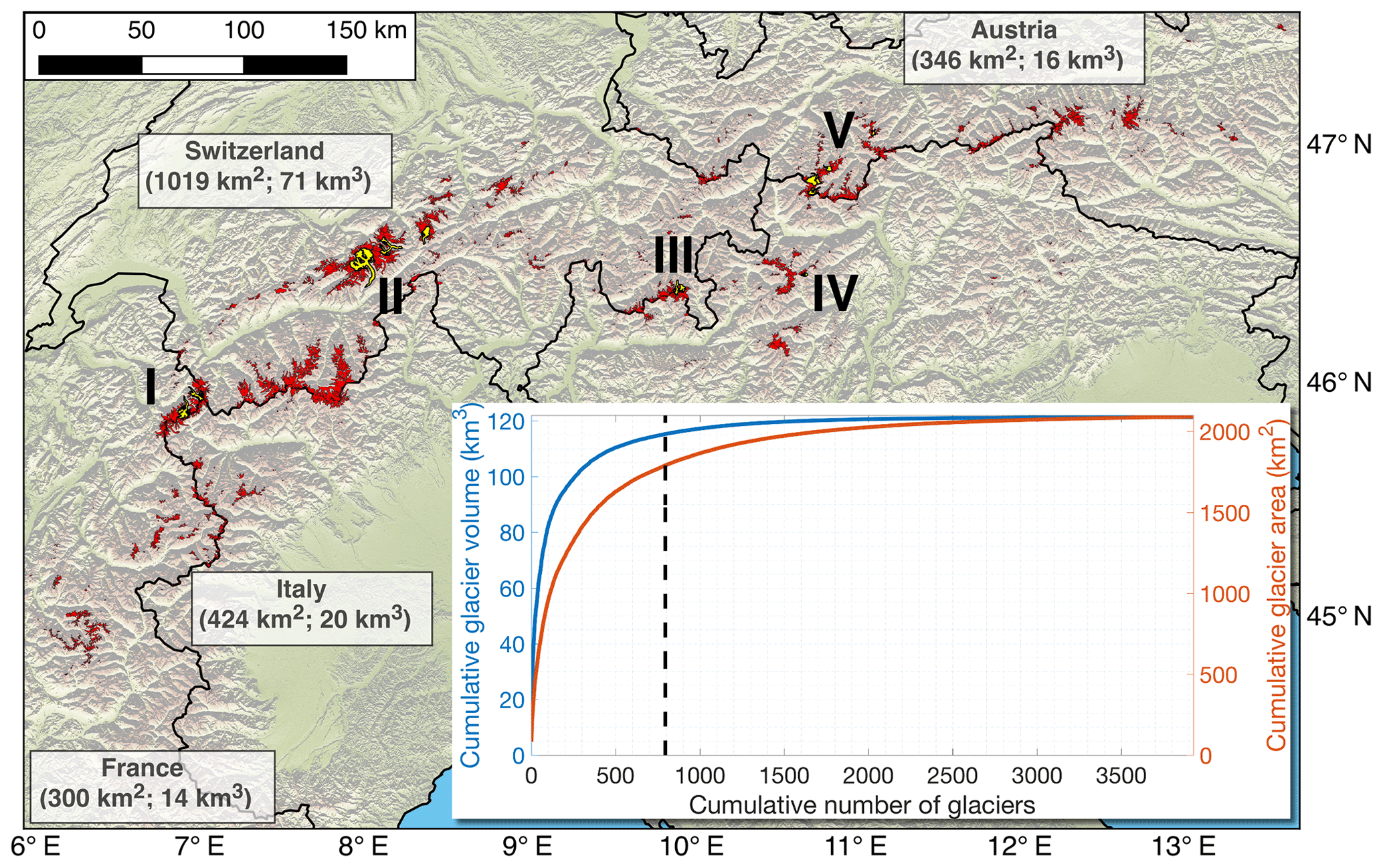
Figure 1Distribution of glaciers (red areas) in the European Alps. Outlines correspond to the glacier geometries at the Randolph Glacier Inventory (RGI v6.0) date (typically 2003) (Paul et al., 2011; RGI Consortium, 2017). The hill shade in the background is from the Shuttle Radar Topography (SRTM) DEM (Jarvis et al., 2008). Glaciers discussed in this paper and the Supplement are highlighted in yellow: (I) Mer de Glace and Argentière, (II) Grosser Aletsch, Unteraar and Rhone, (III) Morteratsch, (IV) Careser, (V) Hintereisferner, Kesselwandferner, Taschachferner, Gepatschferner and Langtaler Ferner. The inset shows the cumulative glacier area and volume, sorted by decreasing glacier length. The dotted line is the division between glaciers longer (left) and shorter (right) than 1 km. Glacier area is from the Randolph Glacier Inventory (RGI v6.0) (RGI Consortium, 2017); volume and length are as derived from an updated version of Huss and Farinotti (2012).
For certain well-studied Alpine glaciers, 3-D high-resolution ice flow models have been used to simulate their future evolution (e.g. Le Meur and Vincent, 2003; Le Meur et al., 2004, 2007; Jouvet et al., 2009, 2011; Zekollari et al., 2014). These studies are of large interest to better understand the glacier dynamics and the driving mechanisms behind their future evolution, but individual glacier characteristics hamper extrapolations of these findings to the regional scale (Beniston et al., 2018). Given the computational expenses related to running such complex models, and due to the lack of field measurements needed for model calibration and validation (e.g. mass balance, ice thickness and surface velocity measurements), these models cannot be applied for every individual glacier in the European Alps. A possible alternative consists of using a regional glaciation model (RGM), in which a surface mass balance (SMB) component and an ice dynamics component are coupled and applied over an entire mountain range, i.e. not for every glacier individually (Clarke et al., 2015). However, running a RGM at a high spatial resolution remains computationally expensive, and the discrepancy between the model complexity and the uncertainty in the various boundary conditions persists. In an RGM study for western Canada, Clarke et al. (2015) showed that relative area and volume changes are well represented by such a model but that large, local present-day differences between observed and modelled glacier geometries can exist after a transient simulation. To date, the most adequate and sophisticated method to model the evolution of all glaciers in the European Alps thus consists of modelling every glacier individually with a coupled ice flow–surface mass balance model. A pilot study in this direction was undertaken by Maussion et al. (2019), with the newly released Open Global Glacier Model (OGGM), in which steady-state simulations are performed for every glacier worldwide based on standard (i.e. non-calibrated) model parameters under the 1985–2015 climate. This model was recently also used by Goosse et al. (2018) to simulate the transient evolution of 71 Alpine glaciers over the past millennium.
Here, we explore the potential of using a coupled SMB–ice flow model for regional projections, by modelling the future evolution of glaciers in the European Alps with such a model. For this, we extend the Global Glacier Evolution Model (GloGEM) of Huss and Hock (2015) by introducing an ice flow component. We refer to this model as GloGEMflow in the following. Our approach is furthermore novel, as glacier-specific geodetic mass balance estimates are used for model calibration, and the future glacier evolution relies directly on regional climate change projections from the EURO-CORDEX (COordinated Regional climate Downscaling EXperiment applied over Europe) ensemble (Jacob et al., 2014; Kotlarski et al., 2014). This is, to the best of our knowledge, the first regional glacier modelling study in the Alps directly making use of this high-resolution regional climate model (RCM) output. In contrast to a forcing with a general circulation model (GCM), an RCM driven by a GCM can provide information on much smaller scales, supporting a more in-depth impact assessment and providing projections with much detail and more accurate representation of localised events.
Through novel approaches in terms of (i) climate forcing, (ii) inclusion of ice dynamics, (iii) the use of glacier-specific geodetic mass balance estimates for model calibration and by (iv) relying on a vast and diverse dataset on ground-truth data for model calibration and validation, we aim at improving future glacier change projections in the European Alps. As part of our analysis, we explore how the new methods and data utilised could affect other regional and global glacier evolution studies.
2.1 Glacier geometry
For every individual glacier in the European Alps, the outlines are taken from the Randolph Glacier Inventory (RGI v6.0) (RGI Consortium, 2017) (Fig. 1). These glacier outlines are mostly from an inventory derived by Paul et al. (2011) using Landsat Thematic Mapper scenes from August and September 2003 (for 96.7 % of all glaciers included in the RGI). The surface hypsometry is derived from the Shuttle Radar Topography Mission (SRTM) version 4 (Jarvis et al., 2008) digital elevation model (DEM) from 2000 (RGI Consortium, 2017).
The ice thicknesses of the individual glaciers is calculated according to the method of Huss and Farinotti (2012) in 10 m elevation bands, which relies on ice volume flux estimates. The horizontal distance (Δx) between the elevation bands is determined from the elevation difference (Δy) and the band-average local surface slope (s):
To determine the band-average slope s, all values below the 5 % quantile are discarded, as well as all values above a threshold (typically around the 80 % to 90 % quantile) determined based on the skewness of the slope distribution function. Subsequently, the glacier geometry is interpolated to a regular, horizontal grid along-flow. Through this approach, possible glacier branches and tributaries are not explicitly accounted for, avoiding complications and potential problems related to solving the little-known mass transfer in these connections. As such, this approach is less sensitive to uncertainties in glacier outlines and topography compared to methods in which glacier branches are explicitly accounted for (e.g. Maussion et al., 2019) but may in some cases oversimplify the mass flow for complex glacier geometries (e.g. with several branches). Glacier cross sections are represented as symmetrical trapezoids. The bedrock elevation is determined in order to ensure local volume and area conservation. These symmetrical trapezoids deviate from a rectangular cross section by an angle α (see Fig. S1 in the Supplement). A value of 45∘ is taken for α, the effect of which is assessed in the uncertainty analysis (Sect. 6.3).
2.2 Climate data
The 2 m air temperature and precipitation are used to represent the climatic conditions at the glacier surface for SMB calculations (Sect. 3.1). For the past (1951–2017), we rely on the ENSEMBLES daily gridded observational dataset (E-OBS v.17.0) on a 0.22∘ grid (Haylock et al., 2008). This E-OBS product represents past events closely (for example, the heat wave of the summer of 2003; Fig. 2b), allowing for detailed comparisons between observed and modelled surface mass balances (Sect. 4.1). We prefer using an observational dataset compared to a reanalysis product (e.g. ERA-INTERIM, as used in Huss and Hock, 2015), as the former has a higher resolution and goes further back in time. Additionally, relying on higher-resolution RCM simulations forced with reanalysis data is not possible, as for several future simulations (see next section), a related simulation is not available. This would furthermore complicate the model validation for the past, as the past climatic conditions would be different for every model RCM simulation, while the observational data provide a single past temperature and precipitation forcing.
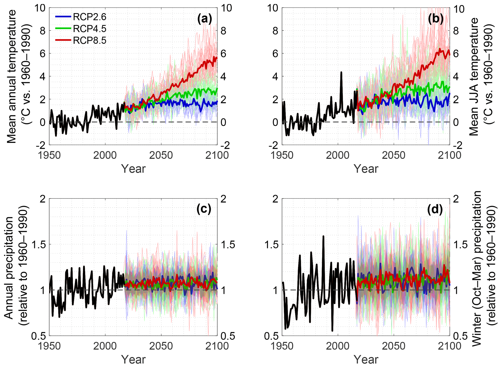
Figure 2Debiased temperature anomaly (a: annual b: June–July–August) and debiased precipitation anomaly (c: annual and d: October–March) between 1950 and 2100 relative to 1961–1990 (horizontal dotted line). All values correspond to the mean over all grid cells used in this study, weighed by the glacier area (at inventory date) in every cell. The thick black line represents the evolution of the variables for observational period (E-OBS dataset). The coloured thin lines represent the evolution for individual RCM simulations from the EURO-CORDEX ensemble (51 in total; see Table S1), and the thick lines are the RCM simulation means (one per RCP).
For the future, we use climate change projections from the EURO-CORDEX ensemble (Jacob et al., 2014; Kotlarski et al., 2014), from which all available simulations at 0.11∘ resolution (ca. 12 km horizontal resolution) are considered. This corresponds to a total of 51 simulations, consisting of different combinations of nine RCMs, six GCMs and various realisations (r1i1p1, r12i1p1, r2i1p1, r3i1p1), forced with three representative concentration pathways (RCPs; Fig. 2 and Table S1 in the Supplement) (van Vuuren et al., 2011; IPCC, 2013). The three considered RCPs are (i) a peak-and-decline scenario with a rapid stabilisation of atmospheric CO2 levels (RCP2.6), (ii) a medium mitigation scenario (RCP4.5) and (iii) a high-emission scenario (RCP8.5). Note that while country-specific projections such as the ones recently released with CH2018 report for Switzerland (CH2018, 2018) exist, which rely on simulations from the EURO-CORDEX ensemble, these cannot be applied in a uniform way over the entire Alps.
For modelling the future SMB, debiased RCM trends from the EURO-CORDEX ensemble are imposed on the E-OBS grid based on the nearest grid cell. To ensure a consistency between the observational (E-OBS, used for past) and RCM (EURO-CORDEX, used for future) climatic data, a debiasing procedure is applied (Huss and Hock, 2015). Here, additive (temperature) and multiplicative (precipitation) monthly biases are calculated to ensure a consistency in the magnitude of the signal over the common time period. These biases are assumed to be constant in time and are superimposed on the RCM series. Furthermore, RCM temperature series are adjusted to account for differences in year-to-year variability between the observational and the RCM time series. Accounting for the differences in interannual variability is crucial to ensure the validity of the calibrated model parameters for the future RCM projections (Hock, 2003; Farinotti, 2013). For each month m, the standard deviation of temperatures over the common time period is calculated for both the observational (σobs,m) and the RCM data (σRCM,m). For each month m and year y of the projection period, the interannual variability of the RCM air temperatures Tm,y is corrected as
Here is the average temperature in a 25-year period centred around y, and ϕm corresponds to . This correction is applied over the period 1970–2017, which is the overlap period for which all RCM simulations and E-OBS data are available. This procedure ensures consistency in interannual variability while allowing for future changes in the temperature variability given by the RCMs (Fig. 2). For precipitation, which enters the SMB calculations as a cumulative quantity, no correction for interannual variability is applied, as the monthly differences in variability are not that relevant at the annual scale. Furthermore, variability in precipitation does not have a direct effect on the calibrated SMB parameters (as is the case for temperatures via the degree-day factors; see Sect. 3.1.).
2.3 Mass balance
The SMB model component is calibrated (Sect. 3.1) with glacier-specific geodetic mass balances taken from the World Glacier Monitoring Service (WMGS) database (WGMS, 2018). Most of these geodetic mass balances were derived by Fischer (2011) (Austria), Berthier et al. (2014) (France, Italy and Switzerland) and M. Fischer et al. (2015) (Switzerland). About 1500 glaciers (ca. 38 % by number) have a glacier-specific geodetic mass balance observation. Since larger glaciers are overrepresented in this sample, however, this corresponds to about 60 % of the total Alpine glacier area. For glaciers for which several geodetic SMB observations are available, the one closest to the reference period 1981–2010 is selected for model calibration. In the case no geodetic mass balance observation for the specific glacier is available, an observation from a nearby glacier is chosen. The respective observation is selected based on (i) the horizontal distance (in km) and (ii) the relative difference in area (unitless). We multiply these two values and consider the minimum as the most suitable glacier to supply a mass balance observation for the unmeasured glacier. The replacement thus represents a nearby glacier that is relatively similar in size. The effect of this approach is evaluated in Sect. 4.1.
For model validation (Sect. 4.1), we rely on in situ SMB observations provided by the WGMS Fluctuations of Glaciers Database (WGMS, 2018), consisting of 1672 glacier-wide annual balances and 12 097 annual balances for specific glacier elevation bands. Note that we prefer using geodetic mass balance over SMB observations for calibration, as we argue that it is more important to have a good coverage for model calibration than for its validation. Furthermore, geodetic mass balances are becoming increasingly available at the regional scale (e.g. Brun et al., 2017; Braun et al., 2019) and outgrow the availability of in situ measurements, making the adopted strategy applicable to other regions.
GloGEMflow consists of a surface mass balance component (Sect. 3.1), which is taken from GloGEM (Huss and Hock, 2015), and an ice flow component (Sect. 3.2). These two components are combined to calculate the temporal evolution of the glacier (Sect. 3.3).
3.1 Surface mass balance modelling
Here, we briefly describe the SMB model component, with an emphasis on the settings specific to this study. For a more elaborate description, we refer to the description in Huss and Hock (2015).
For every glacier, the model is forced with monthly temperature and precipitation series (Sect. 2.2) from the E-OBS (past) or RCM (future) grid cell closest to the glacier's centre point. Accumulation is computed from precipitation, and a threshold is used to differentiate between liquid and solid precipitation. This threshold is defined as an interval from 0.5 to 2.5 ∘C, within which the snow / rain ratio is linearly interpolated. The melt is calculated for every grid cell from a classic temperature-index melt model (Hock, 2003), in which a distinction between snow, firn and ice melt is made based on different degree-day factors. Refreezing of rain and melt water is also accounted for and calculated from snow and firn temperatures based on heat conduction (see Huss and Hock, 2015). Huss and Hock (2015) showed that the added value of using a simplified energy balance model (Oerlemans, 2001) was limited and that it did not perform better than the temperature-index melt model when validated against SMB measurements.
For every individual glacier the climatic data are scaled from the gridded product to the individual glacier at a rate of 2.5 % per 100 m elevation change for precipitation and by relying on monthly temperature lapse rates derived from the RCMs. Subsequently, model calibration parameters (degree-day factors, precipitation scaling factor) are adapted as a part of a glacier-specific three-step calibration procedure that aims at reproducing the observed geodetic mass balance. In the first step, overall precipitation is multiplied by a scaling factor varying between 0.8 and 2.0. This initial step focuses on the precipitation, as this is the variable that is expected to be the most poorly reproduced due to resolution issues, spatial variability and local effects (e.g. snow redistribution) (e.g. Jarosch et al., 2012; Hannesdóttir et al., 2015; Huss and Hock, 2015). If this step does not allow the observed geodetic SMB to be reproduced within a 10 % bound, in a second step the degree-day factors for snow and ice are modified. Here, the degree-day factor of snow is allowed to vary between 1.75 and 4.5 mm d−1 K−1 (default value is 3 mm d−1 K−1; see Hock, 2003), and the degree-day factor of ice is adjusted to ensure a 2:1 ratio between both degree-day factors. In an eventual third and final step, the air temperature is modified through a systematic shift over the entire glacier (see Fig. 2a in Huss and Hock, 2015, for more details).
3.2 Ice flow modelling
The ice flow is modelled explicitly with a flowline model for all glaciers longer than 1 km at the RGI inventory date. These 795 glaciers represent ca. 95 % of the total volume and 86% of the total area of all glaciers in the European Alps (Fig. 1, inset). For glaciers shorter than 1 km, mass transfer within the glacier is limited, and the time evolution is modelled through the Δh parameterisation (Huss et al., 2010b), in line with the original GloGEM setup (Huss and Hock, 2015).
The dynamics of the ice flow component are solved through the Shallow-Ice Approximation (SIA) (Hutter, 1983), in which basal shear (τ) is proportional to the local ice thickness (H) and the surface slope ():
where g=9.81 m s−2 is gravitational acceleration, while the ice density ρ is set to 900 kg m−3. In our model, mass transport is expressed through a Glen (1955) type of flow law, in which the depth-averaged velocity (m a−1) is defined as
Here n=3 is Glen's flow law exponent, and A is the deformation-sliding factor (Pa−3 a−1) that accounts for the effects of the ice rheology on its deformation, sliding and various others effects (e.g. lateral drag). Basal sliding is implicitly accounted for through this approach and not treated separately from internal deformation, given the relatively large uncertainties associated with it. Basal sliding and internal deformation are both linked to the surface slope and the local ice thickness and have been shown to have similar spatial patterns on Alpine glaciers (e.g. Zekollari et al., 2013), justifying an approach in which both are combined (e.g. Gudmundsson, 1999; Clarke et al., 2015).
3.3 Time evolution and initialisation
The glacier geometry is updated at every time step through the continuity equation:
where b is the surface mass balance (m w.e. a−1), and ∇⋅f is the local divergence of the ice flux (). For a transect with a trapezoidal shape, with a basal width wb and a surface width ws (Fig. S1), this becomes (see Oerlemans, 1997)
where D is the diffusivity factor (m2 a−1):
The continuity equation is solved using a semi-implicit forward scheme by relying on an intermediate time step (i.e. sub-time-step update) in which the geometry is updated.
The initialisation consists of closely reproducing the glacier geometry at the inventory date. At first, constant climatic conditions are imposed, until a steady state is obtained, which represents the glacier in 1990 (Fig. 3). These constant climate conditions correspond to the mean SMB under the 1961–1990 climate, to which a SMB perturbation is applied (detailed below). Subsequently, the glacier is forced with E-OBS data and evolves transiently from 1990 until the glacier-specific inventory date (typically 2003). We opt for a 1990 steady-state glacier, as the glaciers in the European Alps were generally not too far off equilibrium around this period, with SMBs for many glaciers being close to zero (Huss et al., 2010a; WGMS, 2018). By imposing a steady state in 1990, the glacier length at the inventory date can be influenced. Methodologically, choosing an initial steady state before 1990 would be problematic, as in this case the glacier geometry would not determine the glacier length at the inventory date anymore, as the period between the steady state and the inventory date exceeds the typical Alpine glacier response time of several years to a few decades (e.g. Oerlemans, 2007; Zekollari and Huybrechts, 2015).
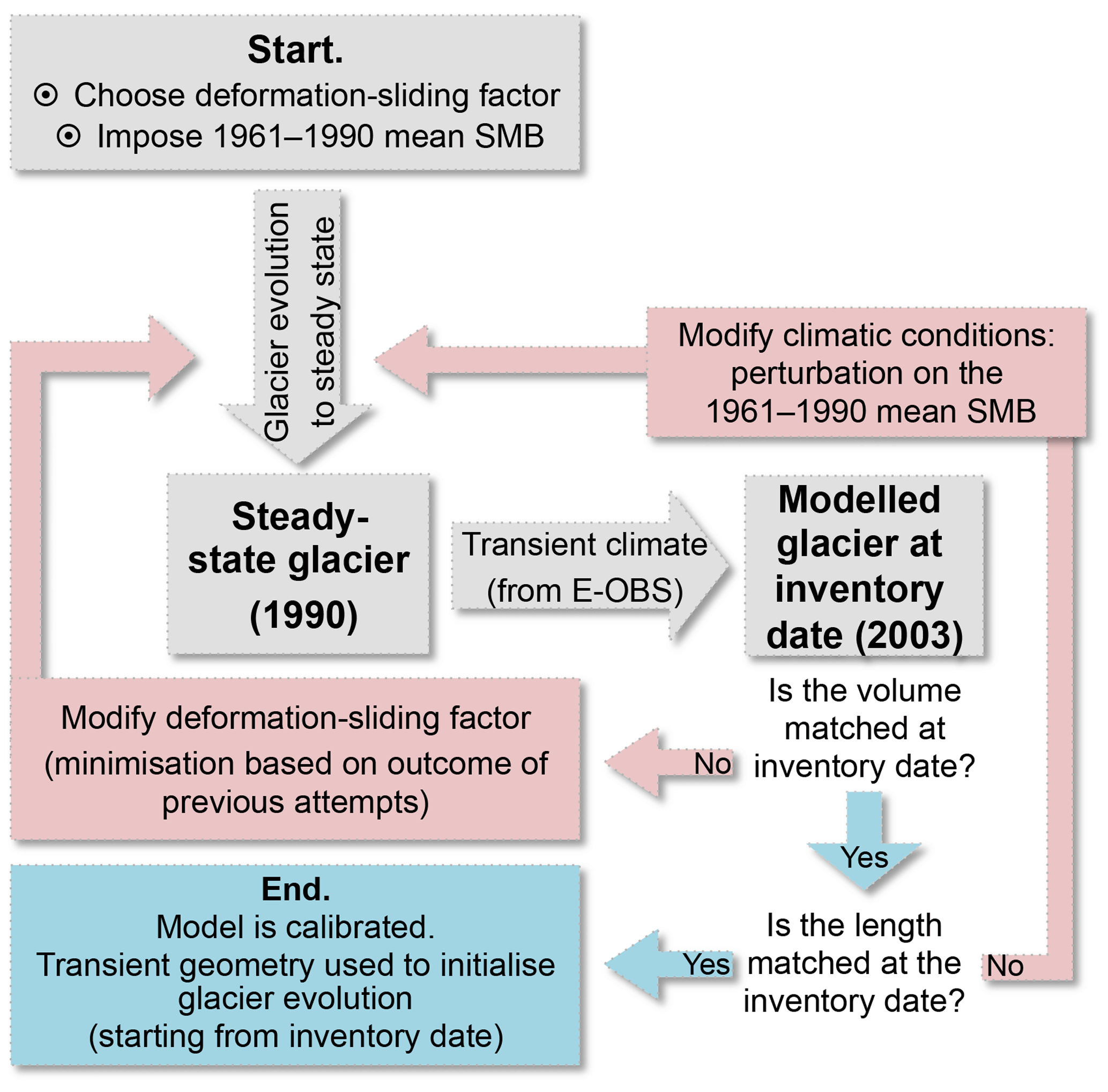
Figure 3Model initialisation for creating a glacier with the reference length and volume at the inventory date.

Figure 4Evaluation of modelled SMB against observations from the WGMS (2018) database. All observations are included, except those that do temporally overlap with the geodetic mass balance observations (used for calibration). Scatterplots (a, c) and frequency of misfits (b, d) of modelled vs. measured glacier-wide annual balances (a, b) and annual mass balances per elevation band (c, d). Dashed red lines in (b) and (d) represent the zero misfit. In (a) and (c), n corresponds to the number of observations, RMSE is the root-mean-square error, MAD is the median absolute deviation and r2 is the coefficient of determination.
The glacier volume and length at the inventory date are matched by calibrating two variables (Fig. 3). The first calibration variable is the deformation-sliding factor A, which mainly determines the volume of the glacier at the inventory date. The reason for this resides in the role that A has on the local ice flux, which in turn affects the local ice thickness and thus the ice volume; see Eqs. (4)–(7). The second calibration variable is an SMB offset in the 1961–1990 climatic conditions used to construct a 1990 steady-state glacier, which mainly determines the length of the steady-state glacier (as the geometry is such that the integrated SMB equals zero). Note that a change in steady-state length causes the glacier length to change at the inventory date as well. An optimisation procedure is used, in which at each iteration the deformation-sliding factor and the SMB offset are informed from previous iterations (see Appendix A for details). This results in a fast convergence to the desired state, i.e. a glacier with the same length and volume as the reference geometry (from Huss and Farinotti, 2012) at the inventory date. It should be noticed that the reference volume is itself a model result (Huss and Farinotti, 2012) and thus also holds uncertainties. The choice for the 1990 steady state and the effect this has on the calibration procedure are assessed in the uncertainty analysis (Sect. 6.3).
4.1 Surface mass balance
The modelled SMB is evaluated by using independent, observed glacier-wide annual balances and annual balances for glacier elevation bands (Fig. 4). In order to ensure that the validation procedure is independent from the calibration, validation is only performed with observations that do not temporally overlap with the geodetic mass balances used for calibration (see Sects. 2.3 and 3.1) and for glaciers without geodetic mass balance observations. As the aim is to evaluate the performance of the SMB model (rather than the coupled SMB–ice flow model) and to incorporate as many validation points as possible (which is only possible after 1990 for the dynamic simulations), these calculations are based on the glacier geometry at the inventory date. The observed glacier-wide annual mass balances are in general well reproduced, with a root-mean-square error (RMSE) of 0.74 m w.e. a−1, a median absolute deviation (MAD) of 0.67 m w.e. a−1 and a systematic error (mean misfit) of −0.09 m w.e. a−1 (Fig. 4a and b). Furthermore, the good agreement between observed and modelled balances for glacier elevation bands (r2=0.60; Fig. 4b and d) suggests that, despite not being calibrated to this, the modelled and observed SMB gradient are in reasonably good agreement. When only considering SMB measurements on glaciers that have no observed geodetic mass balance (i.e. glaciers for which the geodetic mass balance used to calibrate the model was extrapolated from other, nearby glaciers), the misfit between modelled and observed values increases only little (RMSE = 0.79 m w.e. a−1; MAD = 0.72 m w.e. a−1; mean misfit = −0.19 w.e. a−1), indicating that the method used to extrapolate the geodetic mass balances to unmeasured glaciers performs well. Finally, sensitivity tests were performed with the SMB model being forced with historical RCM output (instead of E-OBS). The tests indicate that the RCMs, despite not being forced with reanalysis data, are producing general SMB tendencies that are relatively close to those obtained when forcing the model with E-OBS data (similar mean values; see Fig. S2; similar interannual variability: m w.e. a−1; mean m w.e. a−1).
4.2 Glacier geometry
The glaciers are calibrated to match the length and volume at inventory date within 1 % (σ between reference and modelled volume or length of 0.6 % or 0.5 % of the reference value, respectively). Despite not being calibrated to it, the observed glacier area is also closely reproduced (σ of 0.7 %). In the calibration procedure the distribution of ice with elevation is unconstrained, but nonetheless the reference volume–elevation distribution of various glaciers, based on Huss and Farinotti (2012), updated to RGI v6.0, is well reproduced. We use two well-studied glaciers to illustrate this (Fig. 5), namely the Grosser Aletschgletscher (Valais, Switzerland) and the Mer de Glace (Mont-Blanc massif, France). Also for the other 793 glaciers longer than 1 km, a good match is obtained (see Supplement).
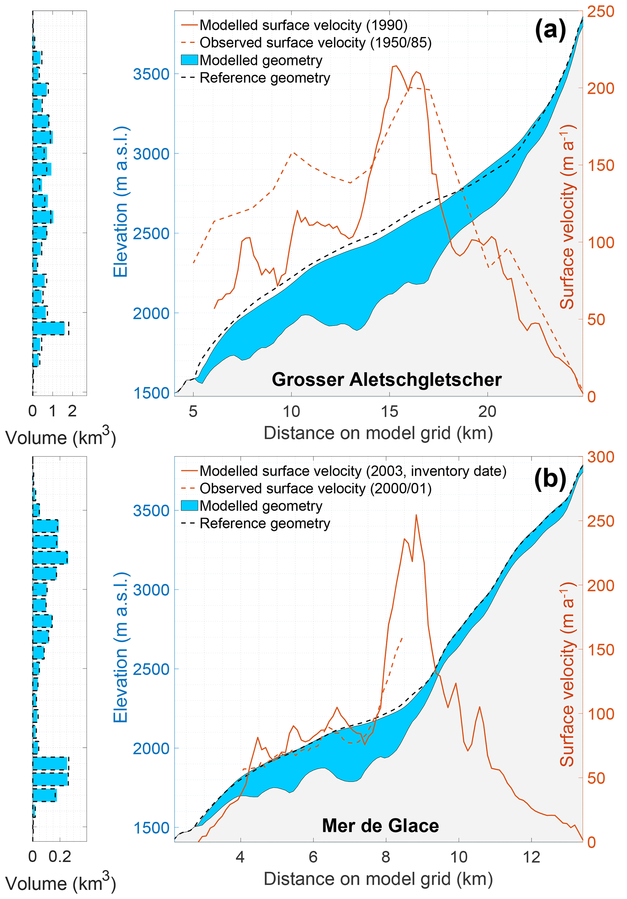
Figure 5Comparison between reference and modelled (i) glacier geometry, (ii) volume–elevation distribution and (iii) surface velocities for Grosser Aletschgletscher (a) and Mer de Glace (b). Reference geometries and volume–elevation distribution are at inventory date (2003) and based on Huss and Farinotti (2012). Observed surface velocities for Grosser Aletschgletscher are from Zoller (2010) and correspond to 1950/1985 point averages, while observed velocities for the Mer de Glace are derived from 2000/2001 SPOT imagery (Berthier and Vincent, 2012).
4.3 Glacier dynamics
In our approach the mass transport between grid cells is linearly dependent on the deformation-sliding factor A, which is thus important for ice dynamics. The calibrated values of A for every individual glacier do not have a distinct spatial pattern, nor do they correlate with glacier length or glacier elevation (Fig. S3). It is not straightforward to compare the values of the deformation-sliding factor to other values from literature used to describe ice deformation and mass transport (such as rate factors), as different formulations and approaches are utilised, e.g. the inclusion/exclusion of a shape factor, explicit/implicit treatment of basal sliding and different geometry representations. However, it appears that the spread in the modelled deformation-sliding factors, which results from the fact that this value represents several physical processes and uncertainties in our approach, largely falls within the literature range values of rate/creep factors (Fig. S3). Furthermore, the calibrated median ( Pa−3 a−1) and mean ( Pa−3 a−1) values are relatively close to the widely used rate/creep factor from Cuffey and Paterson (2010) based on several modelling studies ( Pa−3 a−1).
In the lower parts, where many glaciers have a distinct tongue, a comparison between observed and modelled surface velocities is possible (surface velocities correspond to 1.25 times the depth-integrated velocities, since we treat basal sliding implicitly; see, e.g. Cuffey and Paterson, 2010, p. 310). This is more complicated for the higher parts of the glaciers, where glaciers may be broad and have various branches, which we do not explicitly account for in our approach. In general, our model is able to reproduce the observed surface velocities for the lower glacier parts despite its simplicity. Based on a set of surface velocity observations from the literature (see Fig. 6 and Table S2), a large range of surface velocities, from 1 to >200 m a−1, is well reproduced (r2=0.76; RMSE = 31.8 m a−1), without a tendency for consistent under- or overestimation. This is illustrated for Grosser Aletschgletscher and the Mer de Glace (Fig. 5). Some discrepancies are likely linked to the simplicity of our model and uncertainties in various boundary conditions, but they may in part also be related to the different time periods between the observations and the modelled state.
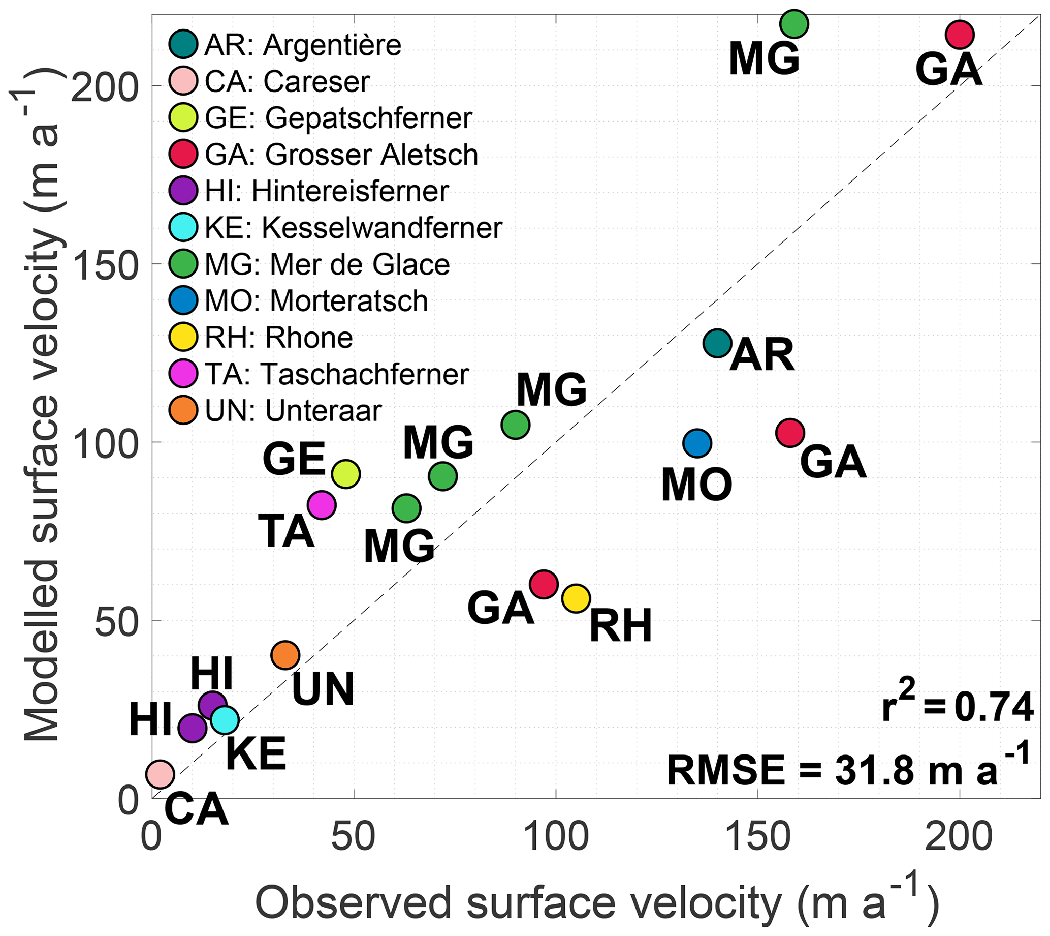
Figure 6Observed vs. modelled surface velocities for selected glaciers in the European Alps. For some glaciers several data points exist, consisting of different locations on the glacier. More information concerning the surface velocities and corresponding references is given in the Supplement (Table S2). For glacier location, see Fig. 1.
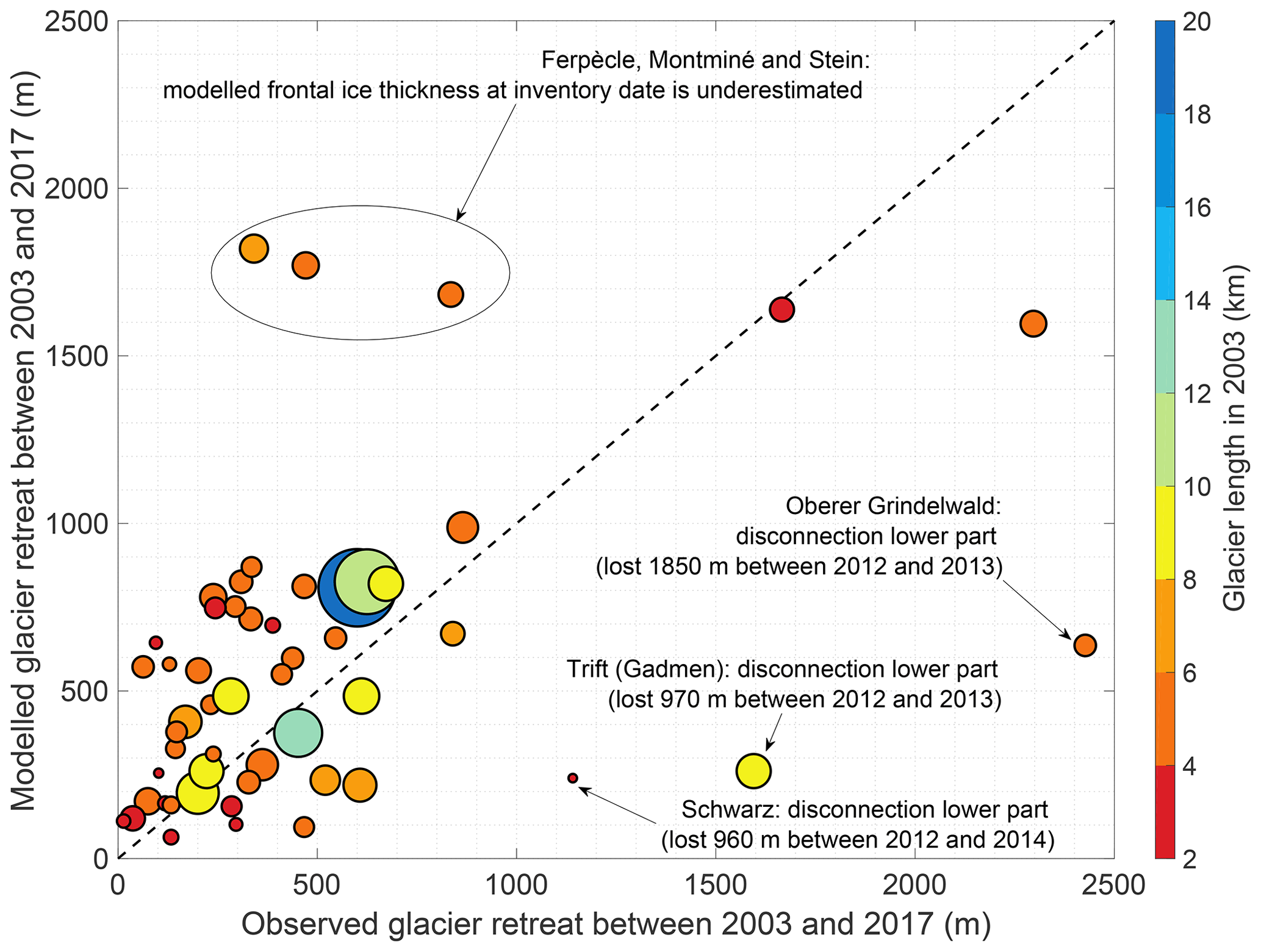
Figure 7Observed vs. modelled glacier retreat (length change) between 2003 and 2017 for all 52 glaciers longer than 3 km monitored by GLAMOS (Glaciological Reports, 1881–2017). Point size is proportional to glacier area (as is the case for the colour bar).
4.4 Past glacier evolution
Modelled past glacier length and area changes are compared to observations for the time period between the inventory date (typically 2003) and present day (2017). Periods before 2003 are not considered, as the effect from the imposed 1990 steady state may still be pronounced on the initial glacier evolution (1990–2003). Furthermore, before the inventory date, length and area changes from the Δh parameterisation (which we apply for glaciers < 1 km) are not available, as here the starting point is the observed geometry at the inventory date. Note that past glacier volume changes are available (e.g. M. Fischer et al., 2015) but that these are not used for validation, as they were utilised for calibrating the SMB model component.
4.4.1 Glacier length
The modelled length changes between the inventory date (2003) and 2017 are compared to observations for all 52 Swiss glaciers longer than 3 km that are included in the Swiss glacier monitoring network (GLAMOS) (Glaciological Reports, 1881–2017) (Fig. 7). Note that other length records are also available for non-Swiss glaciers (e.g. Leclercq et al., 2014) but that these were not considered to ensure a consistency in derived length records. Despite the model's simplicity, the general trends in glacier retreat are relatively well reproduced and there is no general tendency for over- or underestimation. A few outliers exist (highlighted in Fig. 7), of which the underestimations can be attributed to a detachment of the lower and upper parts of the glacier, which cannot be captured in our modelling setup. Overestimated retreat rates (Ferpècle, Montminé and Stein) occur for glaciers where the modelled ice thickness in the frontal region at the inventory date is likely to be lower than the reference state and/or where the ice thickness is underestimated in the reference case. When the three glaciers with underestimations due to a disconnection are omitted, the correlation between the observed and modelled glacier retreat is r2=0.37 (p value < ). For large glaciers, the retreat is particularly well reproduced: e.g. for glaciers longer than 8 km the root-mean-square error (RMSE) between the observed and modelled 2003–2017 retreat is only 155 m, corresponding to approx. 30 % of the mean observed (490 m) and modelled (540 m) retreat over this time period.
4.4.2 Glacier area
Glacier area changes in the European Alps have been derived in various studies. Depending on the time period considered and the ensemble of glaciers studied, estimated glacier area changes vary broadly from −1.5 % a−1 to −0.5 % a−1. Paul et al. (2004) derived area changes for 938 Swiss glaciers and used these to extrapolate a loss of 675 km2 for all glaciers in the European Alps over the period 1973–1998/1999 (corresponding to a 22 % mass loss, or about −0.85 % a−1/26 km2 a−1). For Austria, area changes of −1.2 % a−1 were observed for the period 1998–2004/2012 (A. Fischer et al., 2015). On longer timescales, Fischer et al. (2014) derived a relative area loss of 0.75 % a−1 for the period 1973–2010 over Switzerland, while for the period 2003–2009 an area loss of 1.3 % a−1 was obtained for glaciers in the eastern Swiss Alps. French glaciers lost about one-quarter of their area between 1967/1971 and 2006/2009, corresponding to a change of −0.7 % a−1 (Gardent et al., 2014), while Italian glaciers lost about 30 % of their area over the 1959/1962–2005/2011 period (i.e. average of −0.6 % a−1) (Smiraglia et al., 2015).
Between 2003 and 2017, we model a glacier area loss of 223 km2 (16 km2 a−1), corresponding to a relative area loss of 11.3 % (vs. mean area over this time period), or 0.8 % a−1. These numbers are difficult to directly compare with values from the literature, as different time periods are considered (implying also a different reference area), and as the area losses strongly depend on size of the considered glaciers (e.g. Paul et al., 2004; Fischer et al., 2014), which also varies between studies. However, a qualitative comparison suggests that the modelled area changes are in general slightly lower than the observations. This discrepancy is mostly related to the fact that many present-day glaciers have frontal regions and ablation areas with almost stagnant ice and in some cases also consist of disconnected ice patches, which our model is not able to capture with a simple cross-section parameterisation. By modifying the cross section through increasing λ, a higher modelled area loss is obtained, in closer agreement with observations. However, a higher value of λ may be unrealistic (i.e. produce an area change close to observations for the wrong reasons), and the effect of a different λ value is found to have a very limited effect on the future modelled volume and area changes (this is addressed in Sect. 6.3).
Our projections suggest that from 2017 to 2050 a total volume loss of about 50 % and area loss of about 45 % will occur and that this evolution is independent of the RCP (Fig. 8 and Table 1). This evolution is related to the fact that the annual and summer temperature differences between the RCPs increase with time and are thus relatively limited in the coming decades (see Fig. 2a and b). Furthermore, a part of the future evolution is committed, i.e. being a reaction to the present-day glacier geometry, which is too large for the present-day climatic conditions for most glaciers in the European Alps (e.g. Zekollari and Huybrechts, 2015; Gabbud et al., 2016; Marzeion et al., 2018; see discussion in Sect. 6.1.1).
Table 1Overview of multi-model mean future glacier evolution based on RCM simulations from the EURO-CORDEX ensemble. The evolution under the mean SMB obtained from the 1988–2017 climatic conditions represents the committed loss.
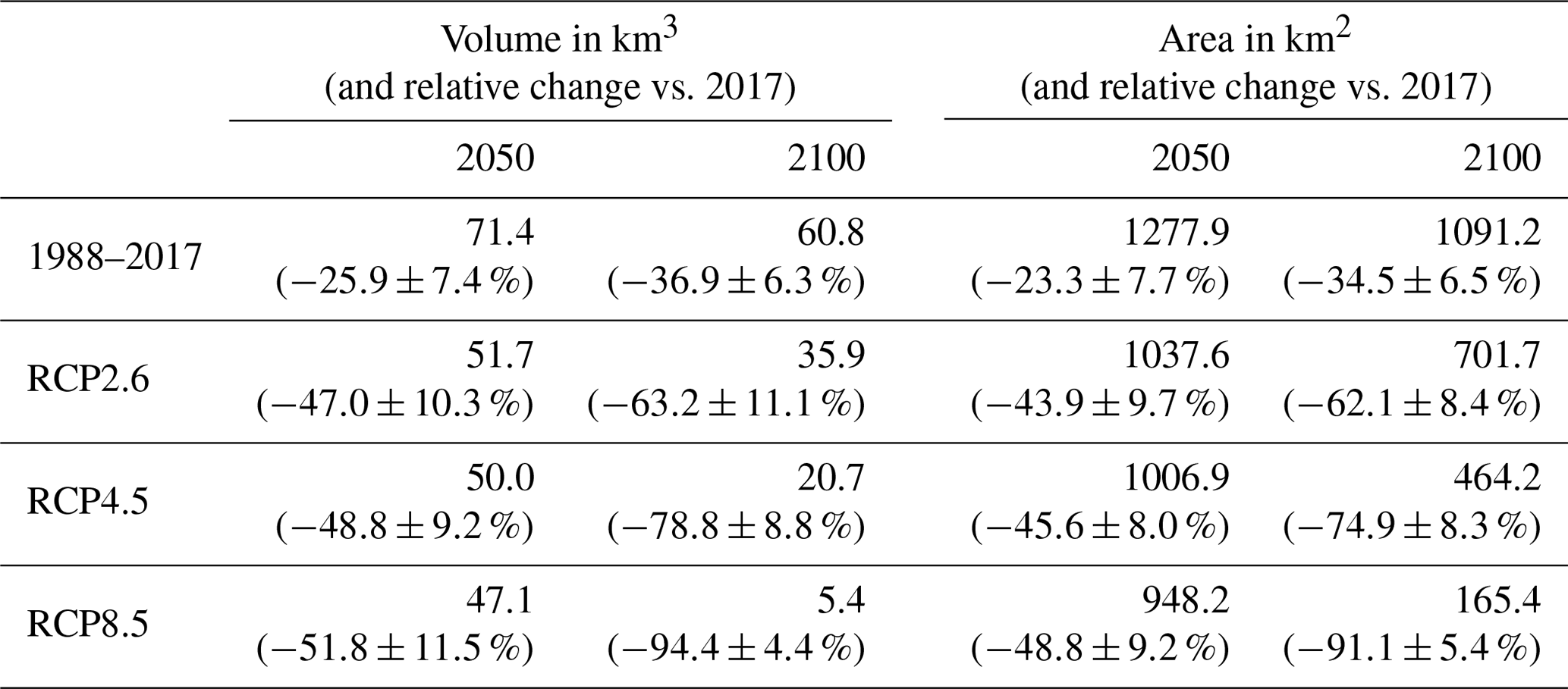
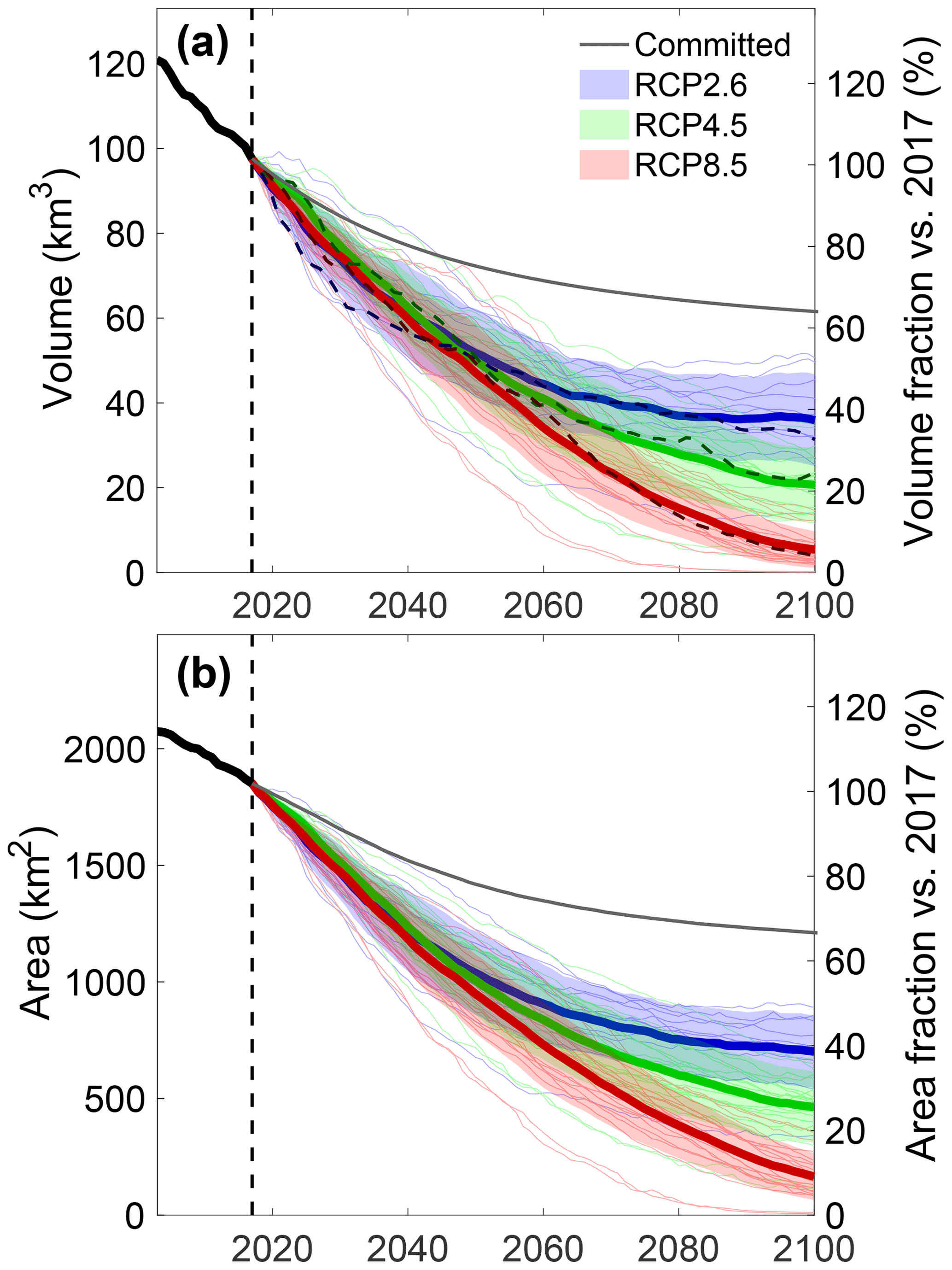
Figure 8Ensemble (a) volume and (b) area evolution for various EURO-CORDEX RCM simulations and committed loss (mean 1988–2017 conditions). Thin lines are individual RCM simulations (51 in total, see Table S1). The thick line is the RCP mean and the transparent bands correspond to one standard deviation. In (a), the coloured dotted lines correspond to the model simulations that are closest to the multi-model mean. The vertical dotted line represents the year 2017 and marks the transition between E-OBS and EURO-CORDEX forcing.
By the end of the century the modelled glacier volume and area are largely determined by the RCP that was used to force the climate model (Fig. 8). Under RCP2.6, in 2100 about 65 % of the present-day (2017) volume and area are lost ( % and % respectively; multi-model mean ±1σ; Table 1, Fig. 8a). Most of the ice loss occurs in the next three decades, corresponding to about 70 %–75 % of the total changes for the period 2017–2100 (Table 1), after which the ice loss clearly reduces (Fig. 8). For an intermediate warming scenario (RCP4.5), about three-quarters of the present-day volume ( %) and area ( %) are lost by the end of the century (Fig. 8, Table 1). In contrast to the glacier evolution under RCP2.6, under RCP4.5 a substantial part of the loss takes place in the second part of the 21st century. However, the largest changes still occur in the coming three decades, with about 60 % of the total changes for the period 2017–2100 (see Table 1). For RCP8.5, the rates of volume loss (−1.5 km3 a−1) and area loss (−25 km2 a−1) are relatively constant until 2070 (Fig. 8), after which they decrease to ca. −0.5 and −15 km2 a−1, respectively. By 2100, the Alps are largely ice-free under RCP8.5, with volume losses of % and area losses of % with respect to 2017 (see Table 1).
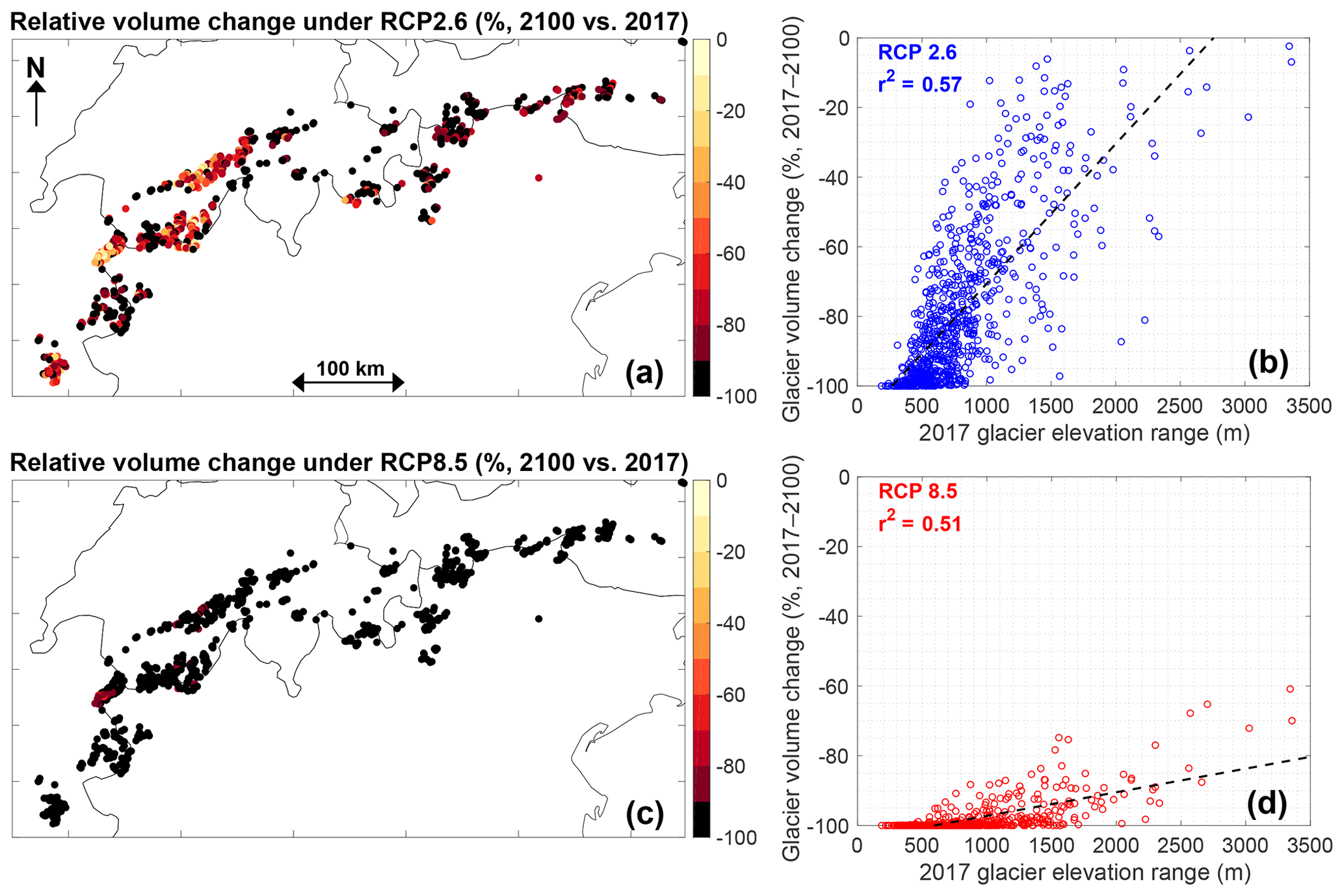
Figure 9Relative volume changes between 2017 and 2100 under RCP2.6 (multi-model mean, a and b) and a RCP8.5 (multi-model mean, c and d). Results are shown for all 795 glaciers for which the future evolution is simulated with the dynamic model. Panels (b) and (d) represent the volume change as a function of the present-day glacier elevation range.
An analysis in which the relative volume loss is compared to present-day glacier characteristics (volume, area, length, median elevation, mean elevation, minimum elevation, maximum elevation, centre of mass and elevation range) reveals that under RCP2.6, the relative volume loss has the highest correlation with the glacier elevation range (Fig. 9 and Table S3; r2=0.57). The maximum glacier elevation, which is strongly related to the glacier elevation range, also describes the volume changes well (Table S3, r2=0.38). This is also evident from the spatial distribution of the relative volume loss, which shows the losses are the lowest for mountain ranges that reach above 3600–3700 m (from west to east): the Écrin massif, the Mont Blanc Massif, the Monte Rosa Massif, the Bernese Alps, the Bernina Range, in the Dolomites, in the Ötzal Alps and the High Tauern (Fig. 9a). The ice loss is particularly strong below 3200 m a.s.l., where (for a given elevation band) more than half of the present-day volume disappears by 2100 under RCP2.6 (Fig. 10). The remaining ice at these lower elevations is typically from medium-sized and large glaciers, which maintain a relatively large accumulation area that supplies mass to the lower glacier regions. This is for instance the case for the Mer de Glace (France) and Grosser Aletschgletscher (Switzerland), where ice is still present below 2500 m a.s.l. by the end of the century under most EURO-CORDEX RCP2.6 simulations (Fig. 11a and b). However, both glaciers lose a considerable part of their length throughout the century, but whereas Grosser Aletschgletscher (Fig. 11a) will likely still be retreating by the end of the century, the Mer de Glace will be relatively stable in 2100 under most EURO-CORDEX simulations and under certain simulations even experience readvance episodes after 2080 (Fig. 11b). Glaciers that spread over a higher elevation range are likely to suffer even fewer changes and in some cases only lose their low-lying tongues (Fig. 9b). In contrast, glaciers at low elevation mostly disappear by the end of the century, even under the moderate RCP2.6 scenario. This is illustrated for Langtaler Ferner (Austria), which is situated below 3300 m a.s.l. and is projected to (almost) entirely disappear somewhere between 2050 and 2100 depending on the specific RCM simulation (Fig. 11c).

Figure 10Modelled volume elevation distribution in 2017 and in 2100 under various representative concentration pathways (RCPs). The values in 2100 correspond to the multi-model mean under a specific RCP.
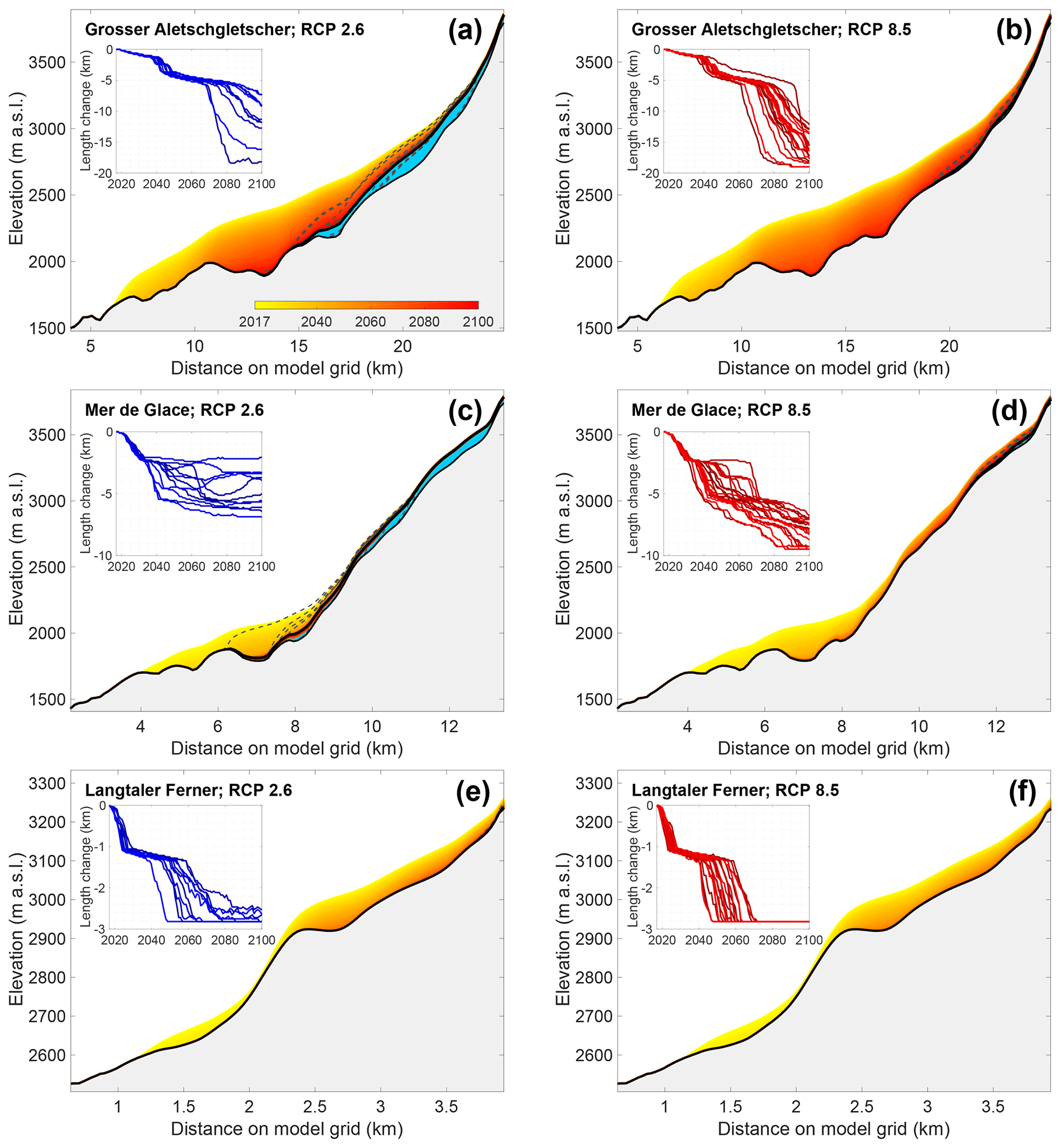
Figure 11Future evolution of the Grosser Aletschgletscher (a, b), Mer de Glace (c, d) and Langtaler Ferner (e, f) under RCP2.6 (a, c, e) and RCP8.5 (b, d, f). The 2017–2100 evolution corresponds to the multi-model mean surface evolution, while the blue area is the multi-model mean glacier geometry at the end of the century. The dotted lines represent the 2100 glacier geometries for individual RCM simulations (see Table S1). The insets represent length changes over the 2017–2100 time period for every individual RCM simulation.
The glacier elevation range is also the variable with the highest correlation with respect to the future relative volume changes under RCP4.5 (r2=0.63) and RCP8.5 (r2=0.51) (Table S3). Under these RCPs, except for the related maximum elevation, also the present-day glacier length correlates significantly () with the 2017–2100 volume loss (r2=0.23 and r2=0.20 respectively). This indicates that under more extreme scenarios the ice loss is very pronounced at all elevations (see also Fig. 11d and e), and the remaining ice in 2100 is mainly a relict of the present-day ice distribution; i.e. ice at the end of the century is only remaining where there is much ice at present at relatively high elevation.
6.1 Drivers of future evolution
6.1.1 Committed loss
Part of the future mass loss is committed and related to the present-day glacier distribution of ice. Many glaciers have a present-day mass excess at low elevation, where locally the flux divergence cannot compensate for the very negative SMB, resulting in a negative thickness change (see Eq. 5 ) (e.g. Johannesson et al., 1989; Adhikari et al., 2011; Zekollari and Huybrechts, 2015; Marzeion et al., 2018). To assess the importance of this committed effect, we investigate the glacier evolution under present-day climatic conditions. For this, the model is constantly forced with the mean 1988–2017 SMB (Fig. 8). Under these conditions, the committed loss is particularly strong for small glaciers at lower elevations (e.g. Langtaler Ferner, with a committed volume loss of ca. 90 % by 2100), while for larger glaciers this effect is more limited. Overall, the Alpine glaciers are projected to lose about 35 % of their present-day volume and area by the end of the century. Simulations with other recent reference periods (e.g. 2008–2017) resulted in similar committed ice losses. This suggests that under RCP2.6, about 60 % of the ice losses for the period 2017–2100 are committed losses, while the remaining 40 % are related to additional warming.
The committed losses are in agreement with simulations performed by Maussion et al. (2019). In steady-state experiments with the Open Global Glacier Model in which all glaciers, starting from their geometry at the inventory date (typically 2003), are subjected to the 1985–2015 randomised climate, Maussion et al. (2019) project ice volume losses of around 55 % over a 100-year time period for the European Alps. In our simulations, over the period 2000–2100, about 50 % of the ice mass is lost for an experiment in which the model is forced with the E-OBS product until 2017 and subsequently with a constant 1988–2017 mean SMB (grey line in Fig. 8a).
6.1.2 Role of ice dynamics
Our model setup allows us to analyse the effect of including ice dynamics, compared to the classic GloGEM setup (Huss and Hock, 2015), in which glacier changes are imposed based on the Δh parameterisation (Huss et al., 2010b) at the regional scale. Comparisons are performed for the period 2003–2100, as the simulations with the Δh parameterisation start from the geometry at the inventory date (2003 for >96 % of all glaciers).
All dynamically modelled glaciers (GloGEMflow) are also run with the Δh parameterisation (GloGEM). A comparison between the (i) difference in the 2003–2100 relative volume loss (between GloGEMflow and GloGEM) and (ii) various glacier characteristics reveals that the effect of including ice dynamics is particularly linked to the glacier elevation range (r2=0.27; ) and to a lesser extent to other (related) glacier characteristics, such as glacier length (r2=0.08), mean slope (r2=0.04), minimum elevation (r2=0.07) and the maximum elevation (r2=0.20) (all values based on multi-model mean for RCP2.6). Under RCP2.6, glaciers with a large elevation range (typically >1000 m) experience less loss in the dynamic model on average compared to when being forced with the Δh parameterisation (Fig. 12). The mechanism behind this is the following:
- i.
At the inventory date, the glacier geometry is very similar in both approaches, as the dynamically modelled glacier is as close as possible to the observed geometry (see Sect. 4.2), which is the starting point for the Δh parameterisation.
- ii.
Initially, the total glacier volume evolution is largely similar in both approaches, as the glaciers are subject to the same climatic conditions, and their geometry does barely differ.
- iii.
However, for glaciers with a large elevation range, relatively more ice is removed at middle and high elevations in the Δh parameterisation, while in the dynamic model the ice loss at the lowest glacier elevations is more pronounced.
- iv.
As a consequence, the geometry starts evolving differently between both approaches, and the larger ice mass at lower elevation in the Δh parameterisation (and lower ice mass at high elevation) translates into a more negative specific glacier mass balance for the Δh parameterisation (vs. the dynamic model), resulting in a higher mass loss.
- v.
In the second half of the 21st century, most glaciers stabilise under a limited to moderate warming (their glacier-wide mass balance evolves towards zero). Given the lower mass and area at middle to high elevations (i.e. around the ELA and higher) for the glaciers modelled with the Δh parameterisation, these glaciers will be slightly smaller to ensure a near-zero SMB.
As glaciers with a large elevation-range are typically the largest glaciers, which make up for a substantial fraction of the total volume, the overall mass loss is thus attenuated when ice dynamics are considered compared to simulations with the Δh parameterisation (Fig. 13, Table S4). The same holds under RCP4.5 (Fig. S4a and b), though being less pronounced due to the more intense melting, which also causes glacier changes to occur at higher elevation. Under RCP8.5, the difference between the dynamically modelled glaciers and those modelled with the Δh parameterisation is almost inexistent (Figs. S4c, d and 13).

Figure 12Future glacier evolution under RCP2.6 for individual glaciers with the dynamic model and corresponding glacier simulation with the Δh parameterisation. All values correspond to RCP2.6 multi-model mean values.
6.1.3 Role of glacier-specific geodetic mass balance estimation
In this study we use direct geodetic mass balance observations from individual glaciers to calibrate the SMB model component. This contrasts with the original GloGEM setup (Huss and Hock, 2015), in which the calibration is based on regional mass balance estimates. To assess the effect of the SMB calibration source, we perform additional simulations in which the model is forced with a region-wide average geodetic mass balance estimate. In order to allow for a direct comparability, we use a region-wide estimate based on the same geodetic mass balance data as used for our glacier-specific calibration. A value of −0.54 m w.e. a−1 is obtained for the period 1981–2010.
Compared to the reference simulations (with the SMB model calibrated using glacier-specific geodetic mass balances), the simulations in which a region-wide SMB estimate is used for model calibration result in a lower future mass loss (Fig. 13, Table S4). The difference is the largest under RCP2.6, in which the glacier volume change for the 2003–2100 period is −65 % (vs. −70 % in the standard simulation). The lower mass loss results likely from the fact that for larger glaciers the region-wide SMB estimate is typically higher than their mass balance. By utilising region-wide estimates, the mass balance is thus overestimated in general for these glaciers that make up for a large fraction of the total volume, resulting in a lower mass loss.
6.1.4 Simulated future climate
To assess the role of climate in the modelled future glacier state, we performed a multilinear regression analysis for categorical data between the RCM simulation characteristics (RCP, RCM, GCM and realisation) and the glacier volume in 2100. In such an analysis, all independent variables are replaced by dummy variables, which have a value of 1 when the variable is considered, and are equal to zero otherwise (e.g. Liang et al., 1992; Tutz, 2012). An analysis in which all possible linear combinations are considered explains most of the variations in the 2100 volume, as the degrees of freedom are relatively low (Table S5). An analysis of variance suggests that most of the variance is described by the RCP (Table S5; p value of F test < 10−3), as expected, and is described earlier (see Fig. 8). The only other term that is significant at the 1 % level is the GCM (), followed by the RCM, which is significant at the 5 % level (p=0.04), and finally the realisation (p=0.13) (Table S5). This indicates that modelled future glacier evolution depends more strongly on the driving GCM than the RCM and that the realisation has a non-significant effect. The importance of the GCM forcing also appears from additional simulations in which the original, low-resolution GCM output was used as model forcing. When comparing these GCM-forced simulations with the corresponding GCM–RCM-forced simulations, the rate of volume loss is slightly higher in the GCM-forced simulations in the early second part of the 21st century, but in 2100 a relatively similar glacier volume is obtained (with relative volume losses compared to the present day typically differing <10 %; Fig. S5).
6.2 Comparison to projections from other Alpine glacier modelling studies
The future evolution of glaciers in the European Alps has been modelled with models of various complexity and by relying on diverse climate projections. By using a statistical calibrated model in which the ELA is related to summer temperature and winter precipitation, Zemp et al. (2006) estimated an area loss of about 40 %, 80 % and 90 % for a respective temperature increase of 1, 3 and 5 ∘C (2100 vs. 1971–1990 mean). Based on 50 glaciers modelled with a retreat parameterisation and subsequent extrapolation, Huss (2012) found that between 4 % (RCP8.5) and 18 % (RCP2.6) of the glacier area will remain by 2100 (vs. 2003). Results from global studies relying on volume–length–area scaling (Marzeion et al., 2012; Radić et al., 2014) and methods in which geometry changes are parameterised (Huss and Hock, 2015) suggest that Alpine glaciers will be subject to volume changes of about −65 % to −80 % under RCP2.6, between −80 % and −90 % under RCP4.5 and around −90 % to −98 % under RCP8.5 (all values between refer to time period between about 2000 and 2100).
Our simulated volume changes are situated between the lowest (Marzeion et al., 2012) and the highest (Huss and Hock, 2015) projected volume losses existing in the literature and are relatively close to the estimates of Radić et al. (2014) (Fig. 14; all changes are considered over the same reference period as studies from the literature). Given the different models and inputs, a direct comparison to the results of Marzeion et al. (2012) and Radić et al. (2014) is difficult. Differences in initial volume estimates may play an important role (e.g. Huss, 2012) and so does the climatic forcing and translation into mass balance, which is study-dependent. The lower losses compared to the results of GloGEM (Huss and Hock, 2015) suggest that the effect of including ice dynamics (reducing the mass loss; Sect. 6.1.2), combined with a slightly lower temperature increase (from EURO-CORDEX RCM ensemble vs. CMIP5 simulations over Europe used in Huss and Hock, 2015), dominates over the effect of using glacier-specific geodetic mass balances (Sect. 6.1.3).

Figure 13Future glacier volume evolution as simulated with (i) the dynamic model forced with an SMB calibrated to individual glaciers (standard run), (ii) the Δh parameterisation (Huss et al., 2010b) and (iii) the dynamic model, for which the SMB model component is calibrated with a region-wide MB estimate. Results are shown for glaciers longer than 1 km at inventory date and correspond to the multi-model values from RCM simulations from the EURO-CORDEX ensemble (for a given RCP).

Figure 14Modelled volume changes and comparison with values from the literature (Marzeion et al., 2012; Radić et al., 2014; Huss and Hock, 2015). The considered time period is in line with the considered study and spans from the early 21st century to 2100.
To the best of our knowledge, three studies have been performed in which the future evolution of an individual Alpine glacier is simulated with 3-D simulations accounting for longitudinal stresses, i.e. with higher-order and full-Stokes models (Jouvet et al., 2009, 2011; Zekollari et al., 2014). Simulations with our flowline model agree well with those for the Rhonegletscher and Grosser Aletschgletscher (Jouvet et al., 2009, 2011) and project a slightly higher mass loss compared to those for the Vadret da Morteratsch complex (Zekollari et al., 2014). A detailed comparison between our simulations and those performed in the detailed studies is provided in the Supplement (Table S6). Given the differences in boundary conditions and model specifications (e.g. bedrock geometry and SMB model) these findings should not be overinterpreted but give a qualitative indication that our model is able to reproduce changes obtained from more complex and detailed studies on individual ice bodies relatively well.
6.3 Sensitivity experiments and uncertainty analysis
6.3.1 1990 steady-state assumption and deformation-sliding factor
In order to assess the effect of the 1990 steady-state assumption and the specific calibration procedure utilised in this study, we performed alternative simulations starting in 1950, in which only the volume at the inventory date is matched (no check on glacier length) through a modification of the deformation-sliding factor. Through this approach, the calibrated deformation-sliding factor is lower than in the two-step approach used as the reference (mean value of Pa−3 a−1 vs. Pa−3 a−1; see Fig. S3), and as such, this experiment also provides insight into the effect of variations in the deformation-sliding factor on future evolution. This is furthermore of interest, as the deformation-sliding factor depends on the reference glacier volume, which is itself a model result (Huss and Farinotti, 2012) with its own uncertainties. The lower deformation-sliding factors (vs. the two-parameter calibration approach) result in slightly shorter glaciers at present (vs. observations), as they represent the same volume at the inventory date. As a consequence, the glaciers are located slightly higher and have a somewhat less pronounced future ice loss (Fig. 15). Despite this, the effect on future evolution is rather limited: under RCP2.6 the 2017–2100 difference in computed volume change is on the order of 5 % between classic volume-length calibration and the “volume-only calibration”. Under RCP4.5 and RCP8.5 the differences in calibration procedure and rate factors barely translate into different 2100 volumes.
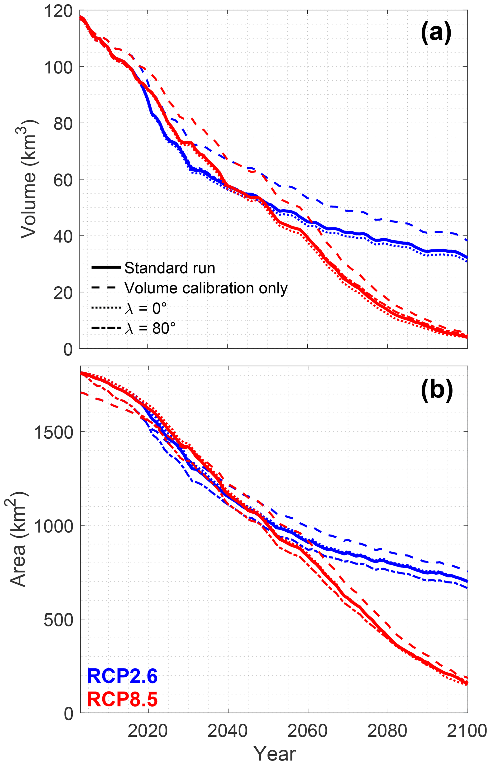
Figure 15Sensitivity of volume (a) and area (b) for different cross-sectional geometries and under a different calibration procedure. Results are shown for all 795 glaciers for which the future evolution is simulated with the dynamic model. The standard calibration with λ=45∘ corresponds to the classic setup. The colours correspond to different RCPs. Only the RCM simulation closest to the multi-model mean volume evolution is shown (dotted line in Fig. 8a; see also Table S1).
6.3.2 Glacier cross section
In all simulations, a trapezoidal cross section with an angle λ of 45∘ was used (Fig. S1). Simulations with a very pronounced trapezium shape (λ=80∘), close to a V-shaped valley, result in larger area changes for the period 2003–2017 of −1.2 % a−1, which is in better agreement with observations (−0.8 % a−1 in classic case) (Fig. 15b). However, in the longer term, the effect on the volume and area loss is very limited, and the area in 2100 is only slightly lower compared to the standard run (λ=45∘), typically on the order of 2 %–3 % (vs. present-day area; Fig. 15b). The same holds for the volume, which is about 2 % lower (vs. present-day volume; Fig. 15a). In the case of a rectangular cross section (λ=0∘), the differences in projected volume and area changes are also very small (on the order of 1 %–2 %) compared to the standard run (λ=45∘). This is in line with the results obtained in the original GloGEM study (Huss and Hock, 2015) on the global scale, in which sensitivity tests with other cross-sectional shapes suggested that projected mass losses would change by 1 %–4 %.
In general, our results indicate that the differences in projected volume and area changes from the various RCM simulations (for a given RCP) are much larger than differences obtained from model parameters. This is in agreement with other glacier evolution studies, as for instance highlighted by Goosse et al. (2018) on the centennial glacier length fluctuation modelling of an ensemble of alpine glaciers with OGGM and by Marzeion et al. (2012), who also find that the ensemble spread within each RCP is the biggest source of uncertainty for the modelled future mass changes.
In this study, we extended an existing glacier evolution model (GloGEM) through the incorporation of an ice flow component. The model extended in this way, GloGEMflow, was used to simulate the future evolution of individual glaciers in the European Alps. In contrast to previous simulations over the European Alps, we used a glacier-specific geodetic mass balance estimate for model calibration. A new initialisation procedure was proposed in which model parameters were calibrated to match the reference glacier length and volume at the inventory date. This novel model setup and its calibration were validated with a broad range of in situ data, including SMB measurements, glacier length changes, glacier area changes and ice surface velocity measurements.
The calibrated model was used to simulate the future evolution of the glaciers in the European Alps under high-resolution RCM future climate scenarios from the EURO-CORDEX ensemble. These simulations of future glacier change can be of interest for various applications (e.g. runoff projections, hydroelectricity production, natural hazards and touristic value) and are available in the Supplement. Our simulations indicated that under RCP2.6, by 2100 about two-thirds of the present-day glacier volume ( %) and area ( %) will be lost. Under a strong warming, the European Alps will be largely ice-free by the end of the century, with projected volume losses of % under RCP4.5 and % under RCP8.5 (2017–2100 period). The future glacier evolution is mostly controlled by the imposed RCP. For a given RCP, the spread in future projections from different RCM simulations is mainly determined by the driving GCM (rather than the RCM) and was found to be much larger than the differences resulting from model parameter variability.
This study focused on the European Alps, for which a vast dataset on glacier data is available. By relying on this unique dataset and by combining it with a novel glacier modelling setup, we were able to quantify a part of the uncertainties related to assumptions that are widely used in regional and global glacier modelling studies, such as the use of region-wide SMB estimates for model calibration and the implicit treatment of ice dynamics. The inclusion of ice dynamics reduced the projected ice loss compared to simulations relying on a retreat parameterisation, and this effect was found to be particularly important for glaciers that extend over a large elevation range. This implies that the inclusion of ice dynamics is likely to be important for global glacier evolution projections, indicating that there is still a relatively large potential to improve these projections.
The following material is available in the Supplement: (1) supplementary tables and figures, (2) the modelled glacier geometries at inventory date for all dynamically modelled glaciers as individual figures and (3) the modelled future (2017–2100) glacier volume evolution for every individual glacier (multi-model mean for RCP2.6, RCP4.5 and RCP8.5) as comma-separated value files (.csv). All other data presented in this paper are available upon request.
As a first guess, a deformation-sliding factor of Pa−3 a−1 is used (A1). This is combined with a SMB bias, which is expressed as a change in ELA (ΔELA1) and chosen in order to ensure a zero mass balance over the present-day glacier geometry. These parameter values are imposed until a steady-state glacier is obtained, and this geometry is subsequently used to model the glacier evolution between 1990 and the inventory date (typically 2003) (Fig. 3). After the first step, a glacier with a volume V1 is obtained. Subsequently, this setup is repeated by modifying the deformation-sliding factor, until the reference glacier volume at the inventory date (Vref) is matched (within 1 %). The second guess for the deformation-sliding factor (A2, i.e. second step of optimisation procedure) corresponds to
Subsequent guesses of A are derived from a polynomial fit between glacier volume (independent variable) and all previous estimates of A (dependent variable). The order of this polynomial fit corresponds to the number of previous guesses minus 1; e.g. the third guess for A relies on the previous two iterations, for which a first-order polynomial (i.e. a linear function) is constructed. This leads to a quick convergence to reference glacier volume at inventory date, typically within 3–4 iterations.
Once a match for the glacier volume is obtained, a check on the glacier length is performed. If the glacier length (L1) deviates more than 1 % from the reference glacier length (Lref), the volume calibration is reapplied, for which the ELA bias (ΔELA1) is increased or decreased with 10 m. The volume calibration is repeated (see above), whereby the first guess for the deformation-sliding factor is now equal to the last guess that resulted in a volume match. Once the volume is matched (typically within one or two iterations), a new check on the glacier length at inventory date is performed. If the length is not matched at the second iteration, from the third iteration onwards, the ΔELA is estimated based on a linear fit between the previous two iterations (independent variables) and the glacier length (dependent variables), or a shift of 10 m if both iterations resulted in the same glacier length (which can occur due to the discretisation of the glacier geometry). All together, this methodology results in a fast convergence, and in general the entire simulation (creating a steady state and running glacier from 1990 to inventory date) needs to be performed about 3–10 times. This takes on average about 10–20 s per glacier on a single core on a modern laptop.
The supplement related to this article is available online at: https://doi.org/10.5194/tc-13-1125-2019-supplement.
HZ, MH and DF conceived the study. HZ developed the ice flow component, which was coupled to the SMB component developed by MH. HZ developed the calibration algorithm, with inputs from MH and DF. The prognostic simulations were performed by HZ and MH and processed by HZ. The manuscript and figures were drafted by HZ in very close and interactive collaboration with MH and DF.
The authors declare that they have no conflict of interest.
Harry Zekollari acknowledges the funding received from WSL (internal innovative project) and the BAFU Hydro-CH2018 project. We thank the data providers in the ECA & D project, which contributed to the E-OBS dataset. We are also grateful to the groups who participated in the coordinated regional climate downscaling over Europe (EURO-CORDEX) for making their data available. Our thanks also go to the World Glacier Monitoring Service (WGMS) for coordinating and distributing SMB data from various groups and to the Swiss Glacier Monitoring Network (GLAMOS) for making glacier length changes available. Andreas Bauder is thanked for helping retrieving surface velocity measurements, and we are also grateful to Wilfried Haeberli for providing insightful comments on this work. We are very grateful for the in-depth editing by Andreas Vieli and the thoughtful and constructive reviews by Ben Marzeion and Fabien Maussion, which were of great help to improve the paper.
This paper was edited by Andreas Vieli and reviewed by Ben Marzeion and Fabien Maussion.
Adhikari, S., Marshall, S. J., and Huybrechts, P.: On characteristic timescales of glacier AX010 in the Nepalese Himalaya, Bull. Glaciol. Res., 29, 19–29, https://doi.org/10.5331/bgr.29.19, 2011.
Bamber, J. L., Westaway, R. M., Marzeion, B., and Wouters, B.: The land ice contribution to sea level during the satellite era, Environ. Res. Lett., 13, 063008, https://doi.org/10.1088/1748-9326/aac2f0, 2018.
Beniston, M., Farinotti, D., Stoffel, M., Andreassen, L. M., Coppola, E., Eckert, N., Fantini, A., Giacona, F., Hauck, C., Huss, M., Huwald, H., Lehning, M., Lopez-Moreno, J.-I., Magnusson, J., Marty, C., Moran-Tejeda, E., Morin, S., Naaim, M., Provenzale, A., Rabatel, A., Six, D., Stötter, J., Strasser, U., Terzago, S., and Vincent, C.: The European mountain cryosphere: a review of its current state, trends, and future challenges, The Cryosphere, 12, 759–794, https://doi.org/10.5194/tc-12-759-2018, 2018.
Berthier, E. and Vincent, C.: Relative contribution of surface mass-balance and ice-flux changes to the accelerated thinning of Mer de Glace, French Alps, over 1979–2008, J. Glaciol., 58, 501–512, https://doi.org/10.3189/2012JoG11J083, 2012.
Berthier, E., Vincent, C., Magnússon, E., Gunnlaugsson, Á. Þ., Pitte, P., Le Meur, E., Masiokas, M., and Ruiz, L.: Glacier topography and elevation changes derived from Pléiades sub-meter stereo images, The Cryosphere, 8, 2275–2291, https://doi.org/10.5194/tc-8-2275-2014, 2014.
Braun, M. H., Malz, P., Sommer, C., Farias-Barahona, D., Sauter, T., Casassa, G., Soruco, A., Skvarca, P., and Seehaus, T. C.: Constraining glacier elevation and mass changes in South America, Nat. Clim. Change, 9, 130–136, https://doi.org/10.1038/s41558-018-0375-7, 2019.
Brun, F., Berthier, E., Wagnon, P., Kääb, A., and Treichler, D.: A spatially resolved estimate of High Mountain Asia glacier mass balances from 2000 to 2016, Nat. Geosci., 10, 668–673, https://doi.org/10.1038/NGEO2999, 2017.
Brunner, M., Björnsen Gurung, A., Zappa, M., Zekollari, H., Farinotti, D., and Stähli, M.: Present and future water scarcity in Switzerland: Potential for alleviation through reservoirs and lakes, Sci. Total Environ., 666, 1033–1047, https://doi.org/10.1016/j.scitotenv.2019.02.169, 2019.
CH2018: CH2018 – Climate Scenarios for Switzerland, Technical Report, National Centre for Climate Services, Zurich, 2018.
Christidis, N., Jones, G. S., and Stott, P. A.: Dramatically increasing chance of extremely hot summers since the 2003 European heatwave, Nat. Clim. Change, 5, 46–50, https://doi.org/10.1038/nclimate2468, 2015.
Clarke, G. K. C., Jarosch, A. H., Anslow, F. S., Radić, V., and Menounos, B.: Projected deglaciation of western Canada in the twenty-first century, Nat. Geosci., 8, 372–377, https://doi.org/10.1038/ngeo2407, 2015.
Cuffey, K. M. and Paterson, W. S. B.: The physics of glaciers, Butterworth-Heinemann, Oxford, 2010.
Farinotti, D.: On the effect of short-term climate variability on mountain glaciers: Insights from a case study, J. Glaciol., 59, 992–1006, https://doi.org/10.3189/2013JoG13J080, 2013.
Fischer, A.: Comparison of direct and geodetic mass balances on a multi-annual time scale, The Cryosphere, 5, 107–124, https://doi.org/10.5194/tc-5-107-2011, 2011.
Fischer, A., Olefs, M., and Abermann, J.: Glaciers, snow and ski tourism in Austria's changing climate, Ann. Glaciol., 52, 89–96, https://doi.org/10.3189/172756411797252338, 2011.
Fischer, A., Seiser, B., Stocker Waldhuber, M., Mitterer, C., and Abermann, J.: Tracing glacier changes in Austria from the Little Ice Age to the present using a lidar-based high-resolution glacier inventory in Austria, The Cryosphere, 9, 753–766, https://doi.org/10.5194/tc-9-753-2015, 2015.
Fischer, M., Huss, M., Barboux, C., and Hoelzle, M.: The new Swiss Glacier Inventory SGI2010: relevance of using high-resolution source data in areas dominated by very small glaciers, Arct. Antarct. Alp. Res., 46, 933–945, https://doi.org/10.1657/1938-4246-46.4.933, 2014.
Fischer, M., Huss, M., and Hoelzle, M.: Surface elevation and mass changes of all Swiss glaciers 1980–2010, The Cryosphere, 9, 525–540, https://doi.org/10.5194/tc-9-525-2015, 2015.
Frei, P., Kotlarski, S., Liniger, M. A., and Schär, C.: Future snowfall in the Alps: projections based on the EURO-CORDEX regional climate models, The Cryosphere, 12, 1–24, https://doi.org/10.5194/tc-12-1-2018, 2018.
Gabbud, C., Micheletti, N., and Lane, S. N.: Response of a temperate alpine valley glacier to climate change at the decadal scale, Geogr. Ann. A,, 98, 81–95, https://doi.org/10.1111/geoa.12124, 2016.
Gardent, M., Rabatel, A., Dedieu, J. P., and Deline, P.: Multitemporal glacier inventory of the French Alps from the late 1960s to the late 2000s, Global Planet. Change, 120, 24–37, https://doi.org/10.1016/j.gloplacha.2014.05.004, 2014.
Glaciological Reports: The Swiss Glaciers, Yearbooks of the Cryospheric Commission of the Swiss Academy of Sciences (SCNAT) published since 1964 by the Labratory of Hydraulics, No. 1–136, Hydrology and Glaciology (VAW) of ETH Zürich, available at: http://www.glamos.ch. 1881–2017.
Glen, J. W.: The Creep of Polycrystalline Ice, P. Roy. Soc. A, 228, 519–538, https://doi.org/10.1098/rspa.1955.0066, 1955.
Gobiet, A., Kotlarski, S., Beniston, M., Heinrich, G., Rajczak, J., and Stoffel, M.: 21st century climate change in the European Alps – A review, Sci. Total Environ., 493, 1138–1151, https://doi.org/10.1016/j.scitotenv.2013.07.050, 2014.
Goosse, H., Barriat, P.-Y., Dalaiden, Q., Klein, F., Marzeion, B., Maussion, F., Pelucchi, P., and Vlug, A.: Testing the consistency between changes in simulated climate and Alpine glacier length over the past millennium, Clim. Past, 14, 1119–1133, https://doi.org/10.5194/cp-14-1119-2018, 2018.
Gudmundsson, G. H.: A three-dimensional numerical model of the confluence area of Unteraargletscher, Bernese Alps, Switzerland, J. Glaciol., 45, 219–230, https://doi.org/10.3189/002214399793377086, 1999.
Haeberli, W. and Hoelzle, M.: Application of inventory data for estimating characteristics of and regional climate-change effects on mountain glaciers: a pilot study with the European Alps, Ann. Glaciol., 21, 206–212, https://doi.org/10.3189/S0260305500015834, 1995.
Hannesdóttir, H., Aoalgeirsdóttir, G., Jóhannesson, T., Guomundsson, S., Crochet, P., Ágústsson, H., Pàlsson, F., Magnússon, E., Sigurosson, S. P., and Björnsson, H.: Downscaled precipitation applied in modelling of mass balance and the evolution of southeast Vatnajökull, Iceland, J. Glaciol., 61, 799–813, https://doi.org/10.3189/2015JoG15J024, 2015.
Hanzer, F., Förster, K., Nemec, J., and Strasser, U.: Projected cryospheric and hydrological impacts of 21st century climate change in the Ötztal Alps (Austria) simulated using a physically based approach, Hydrol. Earth Syst. Sci., 22, 1593–1614, https://doi.org/10.5194/hess-22-1593-2018, 2018.
Haylock, M. R., Hofstra, N., Klein Tank, A. M. G., Klok, E. J., Jones, P. D., and New, M.: A European daily high-resolution gridded data set of surface temperature and precipitation for 1950–2006, J. Geophys. Res., 113, D20119, https://doi.org/10.1029/2008JD010201, 2008.
Hock, R.: Temperature index melt modelling in mountain areas, J. Hydrol., 282, 104–115, https://doi.org/10.1016/S0022-1694(03)00257-9, 2003.
Huss, M.: Extrapolating glacier mass balance to the mountain-range scale: The European Alps 1900–2100, The Cryosphere, 6, 713–727, https://doi.org/10.5194/tc-6-713-2012, 2012.
Huss, M. and Farinotti, D.: Distributed ice thickness and volume of all glaciers around the globe, J. Geophys. Res.-Earth, 117, F04010, https://doi.org/10.1029/2012JF002523, 2012.
Huss, M. and Hock, R.: A new model for global glacier change and sea-level rise, Front. Earth Sci., 3, 1–22, https://doi.org/10.3389/feart.2015.00054, 2015.
Huss, M. and Hock, R.: Global-scale hydrological response to future glacier mass loss, Nat. Clim. Change, 8, 135–140, https://doi.org/10.1038/s41558-017-0049-x, 2018.
Huss, M., Hock, R., Bauder, A., and Funk, M.: 100-year mass changes in the Swiss Alps linked to the Atlantic Multidecadal Oscillation, Geophys. Res. Lett., 37, L10501, https://doi.org/10.1029/2010GL042616, 2010a.
Huss, M., Jouvet, G., Farinotti, D., and Bauder, A.: Future high-mountain hydrology: A new parameterization of glacier retreat, Hydrol. Earth Syst. Sci., 14, 815–829, https://doi.org/10.5194/hess-14-815-2010, 2010b.
Hutter, K.: Theoretical Glaciology, Reidel Publ. Co., Dordrecht, 1983.
IPCC: Working Group I Contribution to the IPCC Fifth Assessment Report, in: Climate Change 2013: The Physical Science Basis, IPCC, AR5 (March 2013), Cambridge University Press, Cambridge, UK and New York, NY, USA, https://doi.org/10.1017/CBO9781107415324, 2013.
Jacob, D., Petersen, J., Eggert, B., Alias, A., Bøssing, O., Bouwer, L. M., Braun, A., Colette, A., Georgopoulou, E., Gobiet, A., Menut, L., Nikulin, G., Haensler, A., Kriegsmann, A., Martin, E., van Meijgaard, E., Moseley, C., and Pfeifer, S., Preuschmann, S., Radermacher, C., Radtke, K., Rechid, D., Roundsevell, M., Samuelsson, P., Somot, S., Soussana, J.-F., Teichmann, C., Valentini, R., Vautard, R., Weber, B., and Yiou, P.: EURO-CORDEX?: new high-resolution climate change projections for European impact research, Reg. Environ. Change, 14, 563–578, https://doi.org/10.1007/s10113-013-0499-2, 2014.
Jarosch, A. H., Anslow, F. S., and Clarke, G. K. C.: High-resolution precipitation and temperature downscaling for glacier models, Clim. Dynam., 38, 391–409, https://doi.org/10.1007/s00382-010-0949-1, 2012.
Jarvis, A. H. I., Reuter, A., Nelson, A., and Guevara, E.: Hole-filled SRTM for the globe Version 4, available from the CGIAR-CSI SRTM 90 m Database, CGIAR CSI Consort. Spat. Inf., http://srtm.csi.cgiar.org (last access: 1 December 2017), 2008.
Johannesson, T., Raymond, C., and Waddington, E.: Time-scale for adjustment of glaciers to changes in mass balance, J. Glaciol., 35, 355–369, 1989.
Jouvet, G., Huss, M., Blatter, H., Picasso, M., and Rappaz, J.: Numerical simulation of Rhonegletscher from 1874 to 2100, J. Comput. Phys., 228, 6426–6439, https://doi.org/10.1016/j.jcp.2009.05.033, 2009.
Jouvet, G., Huss, M., Funk, M., and Blatter, H.: Modelling the retreat of Grosser Aletschgletscher, Switzerland, in a changing climate, J. Glaciol., 57, 1033–1045, https://doi.org/10.3189/002214311798843359, 2011.
Kotlarski, S., Keuler, K., Christensen, O. B., Colette, A., Déqué, M., Gobiet, A., Goergen, K., Jacob, D., Lüthi, D., van Meijgaard, E., Nikulin, G., Schär, C., Teichmann, C., Vautard, R., Warrach-Sagi, K., and Wulfmeyer, V.: Regional climate modeling on European scales: a joint standard evaluation of the EURO-CORDEX RCM ensemble, Geosci. Model Dev., 7, 1297–1333, https://doi.org/10.5194/gmd-7-1297-2014, 2014.
Leclercq, P. W., Oerlemans, J., Basagic, H. J., Bushueva, I., Cook, A. J., and Le Bris, R.: A data set of worldwide glacier length fluctuations, The Cryosphere, 8, 659–672, https://doi.org/10.5194/tc-8-659-2014, 2014.
Liang, K.-Y., Zeger, S. L., and Qaqish, B.: Multivariate Regression Analyses for Categorical Data, J. Roy. Stat. Soc. B, 54, 3–40, https://doi.org/10.1111/j.2517-6161.1992.tb01862.x57, 1992.
Linsbauer, A., Paul, F., Machguth, H., and Haeberli, W.: Comparing three different methods to model scenarios of future glacier change in the Swiss Alps, Ann. Glaciol., 54, 241–253, https://doi.org/10.3189/2013AoG63A400, 2013.
Marzeion, B., Jarosch, A. H., and Hofer, M.: Past and future sea-level change from the surface mass balance of glaciers, The Cryosphere, 6, 1295–1322, https://doi.org/10.5194/tc-6-1295-2012, 2012.
Marzeion, B., Kaser, G., Maussion, F., and Champollion, N.: Limited influence of climate change mitigation on short-term glacier mass loss, Nat. Clim. Change, 8, 305–308, https://doi.org/10.1038/s41558-018-0093-1, 2018.
Maussion, F., Butenko, A., Eis, J., Fourteau, K., Jarosch, A. H., Landmann, J., Oesterle, F., Recinos, B., Rothenpieler, T., Vlug, A., Wild, T., and Marzeion, B.: The Open Global Glacier Model (OGGM) v1.0, Geosci. Model Dev., 12, 909–931, https://doi.org/10.5194/gmd-12-909-2019, 2019.
Le Meur, E. and Vincent, C.: A two-dimensional shallow ice-flow model of Glacier de Saint-Sorlin, France, J. Glaciol., 49, 527–538, https://doi.org/10.3189/172756503781830421, 2003.
Le Meur, E., Gagliardini, O., Zwinger, T., and Ruokolainen, J.: Glacier flow modelling: A comparison of the Shallow Ice Approximation and the full-Stokes solution, Comptes Rendus Phys., 5, 709–722, https://doi.org/10.1016/j.crhy.2004.10.001, 2004.
Le Meur, E., Gerbaux, M., Schäfer, M., and Vincent, C.: Disappearance of an Alpine glacier over the 21st Century simulated from modeling its future surface mass balance, Earth Planet. Sc. Lett., 261, 367–374, https://doi.org/10.1016/j.epsl.2007.07.022, 2007.
Milner, A. M., Khamis, K., Battin, T. J., Brittain, J. E., Barrand, N. E., and Olafsson, S.: Glacier shrinkage driving global changes in downstream systems, P. Natl. Acad. Sci. USA, 114, 9770–9778, https://doi.org/10.1073/pnas.1619807114, 2017.
Moon, T., Ahlstrøm, A., Goelzer, H., Lipscomb, W., and Nowicki, S.: Rising Oceans Guaranteed: Arctic Land Ice Loss and Sea Level Rise, Curr. Clim. Change Rep., 4, 211–222, 2018.
Oerlemans, J.: A flowline model for Nigardsbreen, Norway: projection of future glacier length based on dynamic calibration with the historic record, Ann. Glaciol., 24, 382–389, 1997.
Oerlemans, J.: Glaciers and climate change, A. A. Balkema, Dordrecht, 2001.
Oerlemans, J.: Estimating response times of Vadret da Morteratsch, Vadret da Palü, Briksdalsbreen and Nigardsbreen from their length records, J. Glaciol., 53, 357–362, https://doi.org/10.3189/002214307783258387, 2007.
Parkes, D. and Marzeion, B.: Twentieth-century contribution to sea-level rise from uncharted glaciers, Nature, 563, 551–554, https://doi.org/10.1038/s41586-018-0687-9, 2018.
Patro, E. R., De Michele, C., and Avanzi, F.: Future perspectives of run-of-the-river hydropower and the impact of glaciers' shrinkage: The case of Italian Alps, Appl. Energy, 231, 699–713, https://doi.org/10.1016/J.APENERGY.2018.09.063, 2018.
Paul, F., Kääb, A., Maisch, M., Kellenberger, T., and Haeberli, W.: Rapid disintegration of Alpine glaciers observed with satellite data, Geophys. Res. Lett., 31, L21402, https://doi.org/10.1029/2004GL020816, 2004.
Paul, F., Frey, H., and Bris, R. L. E.: A new glacier inventory for the European Alps from Landsat TM scenes of 2003: challenges and results, Ann. Glaciol., 52, 144–152, https://doi.org/10.3189/172756411799096295, 2011.
Pfeffer, W. T., Arendt, A. A., Bliss, A., Bolch, T., Cogley, J. G., Gardner, A. S., Hagen, J. O., Hock, R., Kaser, G., Kienholz, C., Miles, E. S., Moholdt, G., Mölg, N., Paul, F., Radić, V., Rastner, P., Raup, B. H., Rich, J., Sharp, M. J., Andreassen, L. M., Bajracharya, S., Barrand, N. E., Beedle, M. J., Berthier, E., Bhambri, R., Brown, I., Burgess, D. O., Burgess, E. W., Cawkwell, F., Chinn, T., Copland, L., Cullen, N. J., Davies, B., De Angelis, H., Fountain, A. G., Frey, H., Giffen, B. A., Glasser, N. F., Gurney, S. D., Hagg, W., Hall, D. K., Haritashya, U. K., Hartmann, G., Herreid, S., Howat, I., Jiskoot, H., Khromova, T. E., Klein, A., Kohler, J., König, M., Kriegel, D., Kutuzov, S., Lavrentiev, I., Le Bris, R., Li, X., Manley, W. F., Mayer, C., Menounos, B., Mercer, A., Mool, P., Negrete, A., Nosenko, G., Nuth, C., Osmonov, A., Pettersson, R., Racoviteanu, A., Ranzi, R., Sarikaya, M. A., Schneider, C., Sigurdsson, O., Sirguey, P., Stokes, C. R., Wheate, R., Wolken, G. J., Wu, L. Z., and Wyatt, F. R.: The Randolph Glacier Inventory: A globally complete inventory of glaciers, J. Glaciol., 60, 537–552, https://doi.org/10.3189/2014JoG13J176, 2014.
Radić, V., Bliss, A., Beedlow, A. C., Hock, R., Miles, E., and Cogley, J. G.: Regional and global projections of twenty-first century glacier mass changes in response to climate scenarios from global climate models, Clim. Dynam., 42, 37–58, https://doi.org/10.1007/s00382-013-1719-7, 2014.
RGI Consortium: Randolph Glacier Inventory – A Dataset of Global Glacier Outlines, Version 6.0, Technical Report, Global Land Ice Measurements from Space, Colorado, USA, Digital Media, https://doi.org/10.7265/N5-RGI-60, 2017.
Salzmann, N., Machguth, H., and Linsbauer, A.: The Swiss Alpine glaciers response to the global “2 ∘C air temperature target”, Environ. Res. Lett., 7, 44001, https://doi.org/10.1088/1748-9326/7/4/044001, 2012.
Slangen, A. B. A., Adloff, F., Jevrejeva, S., Leclercq, P. W., Marzeion, B., Wada, Y., and Winkelmann, R.: A Review of Recent Updates of Sea-Level Projections at Global and Regional Scales, Surv. Geophys., 38, 385–406, https://doi.org/10.1007/s10712-016-9374-2, 2017.
Smiraglia, C., Azzoni, R. S., D'agata, C., Maragno, D., Fugazza, D., and Diolaiuti, G. A.: The evolution of the Italian glaciers from the previous data base to the new Italian inventory. preliminary considerations and results, Geogr. Fis. e Din. Quat., 38, 79–87, https://doi.org/10.4461/GFDQ.2015.38.08, 2015.
Stewart, E. J., Wilson, J., Espiner, S., Purdie, H., Lemieux, C., and Dawson, J.: Implications of climate change for glacier tourism, Tour. Geogr., 18, 377–398, https://doi.org/10.1080/14616688.2016.1198416, 2016.
Stoffel, M. and Corona, C.: Future winters glimpsed in the Alps, Nat. Geosci., 11, 458–460, https://doi.org/10.1038/s41561-018-0177-6, 2018.
Tutz, G.: Regression for categorical data, Cambridge University Press, Cambridge, UK, 2012.
van Vuuren, D. P., Edmonds, J., Kainuma, M., Riahi, K., Nakicenovic, N., Smith, S. J., and Rose, S. K.: The representative concentration pathways: an overview, Climatic Change, 109, 5–31, https://doi.org/10.1007/s10584-011-0148-z, 2011.
Welling, J. T., Arnason, Y., and Olafsdottir, R.: Glacier tourism: a scoping review, Tour. Geogr., 17, 635–661, 2015.
WGMS: Fluctuations of Glaciers Database. World Glacier Monitoring Service, Zurich, Switzerland, https://doi.org/10.5904/wgms-fog-2018-06, 2018.
Zekollari, H. and Huybrechts, P.: On the climate-geometry imbalance, response time and volume-area scaling of an alpine glacier: insights from a 3-D flow model applied to Vadret da Morteratsch, Switzerland, Ann. Glaciol., 56, 51–62, https://doi.org/10.3189/2015AoG70A921, 2015.
Zekollari, H., Huybrechts, P., Fürst, J. J., Rybak, O., and Eisen, O.: Calibration of a higher-order 3-D ice-flow model of the Morteratsch glacier complex, Engadin, Switzerland, Ann. Glaciol., 54, 343–351, https://doi.org/10.3189/2013AoG63A434, 2013.
Zekollari, H., Fürst, J. J., and Huybrechts, P.: Modelling the evolution of Vadret da Morteratsch, Switzerland, since the Little Ice Age and into the future, J. Glaciol., 60, 1208–1220, https://doi.org/10.3189/2014JoG14J053, 2014.
Zemp, M., Haeberli, W., Hoelzle, M., and Paul, F.: Alpine glaciers to disappear within decades?, Geophys. Res. Lett., 33, L13504, https://doi.org/10.1029/2006GL026319, 2006.
Zoller, N.: Fliessbewegung des Grossen Aletschgletschers, Bachelor thesis, ETH Zürich, Zurich, 2010.