the Creative Commons Attribution 4.0 License.
the Creative Commons Attribution 4.0 License.
 | 06 Mar 2020
CMIP5 model selection for ISMIP6 ice sheet model forcing: Greenland and Antarctica
Cécile Agosta
Christopher M. Little
Tore Hattermann
Nicolas C. Jourdain
Heiko Goelzer
Sophie Nowicki
Helene Seroussi
Fiammetta Straneo
Thomas J. Bracegirdle
The ice sheet model intercomparison project for CMIP6 (ISMIP6) effort brings together the ice sheet and climate modeling communities to gain understanding of the ice sheet contribution to sea level rise. ISMIP6 conducts stand-alone ice sheet experiments that use space- and time-varying forcing derived from atmosphere–ocean coupled global climate models (AOGCMs) to reflect plausible trajectories for climate projections. The goal of this study is to recommend a subset of CMIP5 AOGCMs (three core and three targeted) to produce forcing for ISMIP6 stand-alone ice sheet simulations, based on (i) their representation of current climate near Antarctica and Greenland relative to observations and (ii) their ability to sample a diversity of projected atmosphere and ocean changes over the 21st century. The selection is performed separately for Greenland and Antarctica. Model evaluation over the historical period focuses on variables used to generate ice sheet forcing. For stage (i), we combine metrics of atmosphere and surface ocean state (annual- and seasonal-mean variables over large spatial domains) with metrics of time-mean subsurface ocean temperature biases averaged over sectors of the continental shelf. For stage (ii), we maximize the diversity of climate projections among the best-performing models. Model selection is also constrained by technical limitations, such as availability of required data from RCP2.6 and RCP8.5 projections. The selected top three CMIP5 climate models are CCSM4, MIROC-ESM-CHEM, and NorESM1-M for Antarctica and HadGEM2-ES, MIROC5, and NorESM1-M for Greenland. This model selection was designed specifically for ISMIP6 but can be adapted for other applications.


The Greenland and Antarctic ice sheets represent the largest and most uncertain contributions to global sea level rise over multidecadal to millennial timescales. During the last 3 decades, satellite observation captured rapid mass loss from both ice sheets (Velicogna, 2009; Zwally et al., 2011; Khan et al., 2014; Mouginot et al., 2014, 2019; Shepherd et al., 2018). Both atmospheric and oceanic changes have been identified as drivers of observed mass loss, although regional mechanisms vary. For example, rising air temperatures over Greenland lead to increased surface melt, causing direct mass loss (Trusel et al., 2018; Fettweis et al., 2017). Enhanced surface meltwater production also destabilizes the margins of the ice sheet (van den Broeke, 2005; Banwell et al., 2013) and lubricates the ice flow at the bed (Andrews et al., 2014; Kendrick et al., 2018). Ocean interactions with the ice sheet occur in Greenland fjords, where a combination of onshore ocean heat transport, estuarine-type circulation, subglacial meltwater runoff, and calving processes influence glacier terminus position and ice discharge (Straneo and Cenedese, 2015). In Antarctica, most of the ice sheet's mass loss is mediated through floating ice shelves. Melting at the ice shelf underside, which affects ice flow dynamics, is mainly controlled by the extent to which ocean dynamics along the continental margin allow intrusion of offshore ocean heat into the ice shelf cavities, leading to distinct regimes operating in “warm” vs. “cold” continental shelf regions (e.g., Dinniman et al., 2016; Thompson et al., 2018). Rising air temperatures and associated surface melting are thought to be responsible for the collapse of ice shelves around the Antarctic Peninsula (Domack et al., 2005) and subsequent speedup of grounded ice flow (Rignot et al., 2004), while surface melting is currently limited in most other parts of the continent (e.g., Trusel et al., 2013). In the future, increased water vapor transport in a warmer atmosphere may lead to increased surface accumulation in Antarctica (Frieler et al., 2015; Palerme et al., 2017) together with increased melting over Greenland (Franco et al., 2013) and the Antarctic ice shelves (Trusel et al., 2015). Besides this general pattern, the spatial distribution and magnitudes of atmospheric and oceanic contributions to the mass balance of both ice sheets vary greatly and depend on synoptic-scale climate variability and physical processes at regional and smaller scales.
The ice sheet model intercomparison project for CMIP6 (ISMIP6) brings together the ice sheet and climate modeling communities to gain understanding of the ice sheet contribution to sea level rise (Nowicki et al., 2016). Due to the delay in the CMIP6 dataset release, ISMIP6 revised the protocol described in Nowicki et al. (2016) to utilize climate forcing from the CMIP5 dataset (Nowicki, 2019). ISMIP6 conducts stand-alone ice sheet experiments that use space- and time-varying forcing derived from atmosphere–ocean coupled global climate models (AOGCMs) to reflect plausible trajectories for climate projections, building on earlier coordinated experiments which applied ad hoc boundary conditions either constant in time or imposed as an abrupt perturbation (Pattyn et al., 2013; Bindschadler et al., 2013; Levermann et al., 2014). However, this effort requires converting AOGCM output to forcing for ice sheet models, posing several challenges. First, climate models from the Coupled Model Intercomparison Project (CMIP) have a horizontal resolution that is too coarse to accurately represent sharp ice sheet topographic gradients impacting the surface climate of the ice sheet (e.g., melt, wind, precipitation). Ocean components cannot represent narrow fjords connecting the deep ocean and tidewater glaciers around Greenland (Straneo et al., 2012), the ocean eddies involved in poleward heat transport across continental shelves (Stewart et al., 2018), or ocean circulation beneath ice shelves (Asay-Davis et al., 2017). Second, AOGCMs poorly represent polar-specific processes that have a major impact on the ice sheet surface climate (e.g., snowpack evolution, cloud and boundary-layer processes) (Favier et al., 2017).
These limitations can be addressed by using regional climate models adapted for the polar regions. On the atmosphere side, polar-oriented regional climate models (RCMs) have proved to provide more realistic surface climate than direct AOGCM outputs for both the Greenland ice sheet (e.g., Noël et al., 2018; Fettweis et al., 2013) and the Antarctic ice sheet (e.g., van Wessem et al., 2018; Agosta et al., 2019). On the ocean side, a number of models have recently added the capability to represent ice shelf cavities and ice–ocean interactions (e.g., Dinniman et al., 2016). However, ocean simulations are still unable to provide non-biased solutions from a pan-ice-sheet perspective, and they remain computationally expensive, which probably explains the small number of existing projections of ice shelf basal melting (Timmermann and Goeller, 2017; Naughten et al., 2018). Thus, the ISMIP6 steering committee has proposed the following strategy to convert AOGCM outputs into ice sheet forcing: surface forcing is provided by AOGCMs dynamically downscaled with a polar-oriented atmospheric RCM (Fettweis et al., 2017), while ocean forcing is computed by interpolating AOGCMs' ocean temperature onto the continental shelf and by parameterizing ice shelf melt or retreat rates, as detailed in Slater et al. (2019) and Nowicki (2019).
The goal of this study is to recommend a subset of CMIP AOGCMs to produce forcing for ISMIP6 stand-alone ice sheet simulations. This ensemble of AOGCMs aims to capture (i) plausible climate near Antarctica and Greenland over the historical period and (ii) a diversity of atmosphere and ocean warming rates over the 21st century. For evaluating AOGCMs we focus on variables that are inputs of the downscaling methods defined to generate ice sheet forcing. Although it is technically possible to select different AOGCMs for atmosphere and ocean forcing, we choose to use the same climate models across both realms due to their inter-dependence in projections (e.g., Krinner et al., 2014; Bracegirdle et al., 2018). We thus perform a combined assessment of both the atmosphere and ocean components of AOGCMs.
This paper describes the process utilized to select six AOGCMs to provide forcing for each ice sheet. This evaluation combines observational/reanalysis data, metrics from existing studies, and data produced specifically for this study. The methodology to combine distinct metrics for the ocean and atmosphere into a single ranking is detailed in Sect. 2. The models are selected independently for the Antarctic (Sect. 3) and the Greenland (Sect. 4) ice sheets. Finally, we present some of the limitations of the selection procedure and discuss perspectives for future research in Sect. 5.
2.1 General methodology
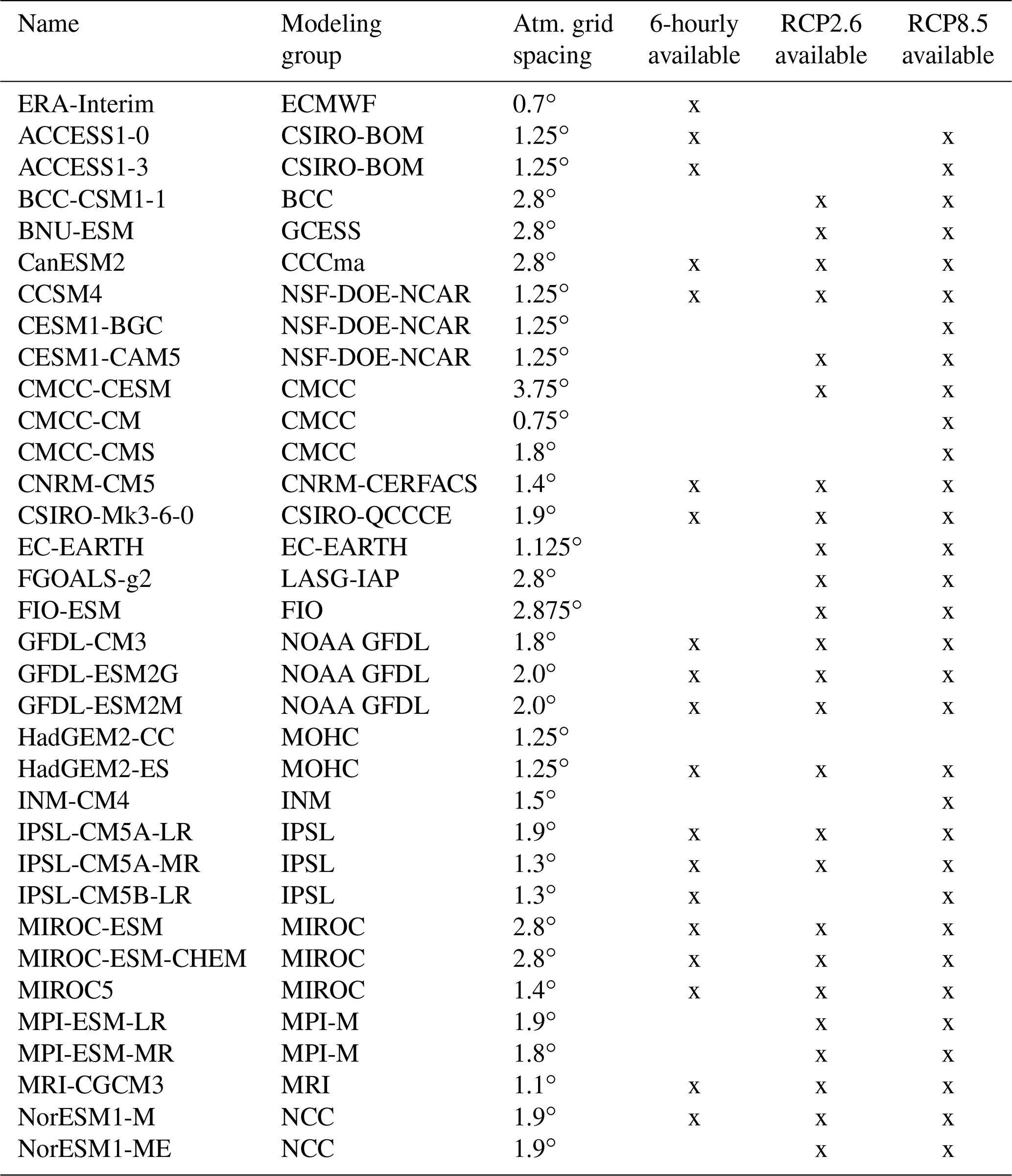
We analyze monthly output from 33 climate models of the CMIP5 ensemble, listed in Table 1. The ISMIP6 stand-alone experiment requires three coupled climate models to derive forcing fields for their core experiments (core), plus three additional models to extend the ensemble to a total of six models (targeted). To select the models, we first rank them according to their performance in reproducing observations over the 1979–2005 historical period (historical metrics, defined in Sect. 2.2). In a second step, we define climate change metrics over the 21st century (21C) under the RCP8.5 scenario (Sect. 2.3.1) in order to select a set of models that represents a diversity of 21C changes (Sect. 2.3.2). This two-step process is performed independently for the Antarctic and Greenland ice sheets.
The top three (core) models are those maximizing the diversity of climate change (Sect. 2.3.2, n=3) among those fitting the following criteria:
-
the model must provide 6-hourly wind, temperature, and humidity to be able to run an atmospheric regional climate model (18 models);
-
the model output must include required data fields under both the RCP2.6 and RCP8.5 scenario projections, following the revised ISMIP6 protocol (Nowicki, 2019) (25 models);
-
the model must rank in the top half of the 33-model ensemble with regard to the historical metrics defined in Sect. 2.2 (17 models, Figs. 2a and 5a);
-
the model must not have any single climate change metric defined in Sect. 2.3.1 above two interquartile ranges (IQR, equal to the 75 % quantile minus the 25 % quantile) from the multi-model median projection (Figs. 4a and 7a).
For the additional three models (targeted), criteria used for the top three are relaxed, now including models without sub-daily frequencies for Antarctica, and including models with projected 21C changes above 2 IQR of the multi-model median. The models are selected to maximize the diversity of climate change across the ensemble of the top six models (Sect. 2.3.2, n=6). As the selection method maximizing diversity tends to favor models with extreme values, we impose one model (within the top six) which features 21C climate changes in the median range of the ensemble.
Table 1ERA-Interim reanalysis and CMIP5 models used in this study.
2.2 Historical metrics
2.2.1 Atmosphere and surface ocean metrics
For the atmosphere and surface ocean, we consider variables that have an impact on RCM-modeled surface mass balance and for which reanalyses are reliable, following Agosta et al. (2015). All model outputs are bilinearly interpolated onto a common regular longitude–latitude grid (). For each variable that retains spatial information (described in the following paragraph), we calculate the spatial root-mean-square error (RMSE) for annual- or seasonal-mean values over 1980–2004 (25 years). We take the European Centre for Medium-Range Weather Forecasts “Interim” re-analysis (ERA-Interim, 1979–present; Dee et al., 2011) as a reference, since differences between reanalyses are much smaller than climate model biases (Agosta et al., 2015), and ERA-Interim was assessed to be the most reliable contemporary global reanalysis over Antarctica (Bromwich et al., 2011; Bracegirdle and Marshall, 2012; Huai et al., 2019).
For Antarctica, we evaluate air temperature at 850 hPa (ta850; average of summer and winter RMSE), annual precipitable water (prw), and annual sea level pressure (psl), together with summer sea surface temperature (sst[s]) and winter sea ice extent (sie[w]), for the domain extending south of 40∘ S over the ocean (Fig. 1a). In addition to spatially resolved variables, we include a metric of the historical CMIP5 vs. ERA-Interim bias in westerly jet strength (Jstr), calculated as the maximum in annual mean zonal mean 850 hPa zonal wind between 10 and 75∘ S (m s−1), compared to time-slice means of the overlapping 1979–2005 period, as in Bracegirdle et al. (2018).
For Greenland, we evaluate air temperature at 700 hPa (ta700; average of summer and winter RMSE), annual precipitable water (prw), and annual geopotential height at 500 hPa (zg500), inside the domain of the “Modèle Atmosphèrique Regional” (MAR; Fettweis et al., 2017) and where the Greenland ice sheet is below 2000 m (bright shaded color in Fig. 1c). In this small domain, sea surface conditions do not significantly impact MAR results (Noël et al., 2014).
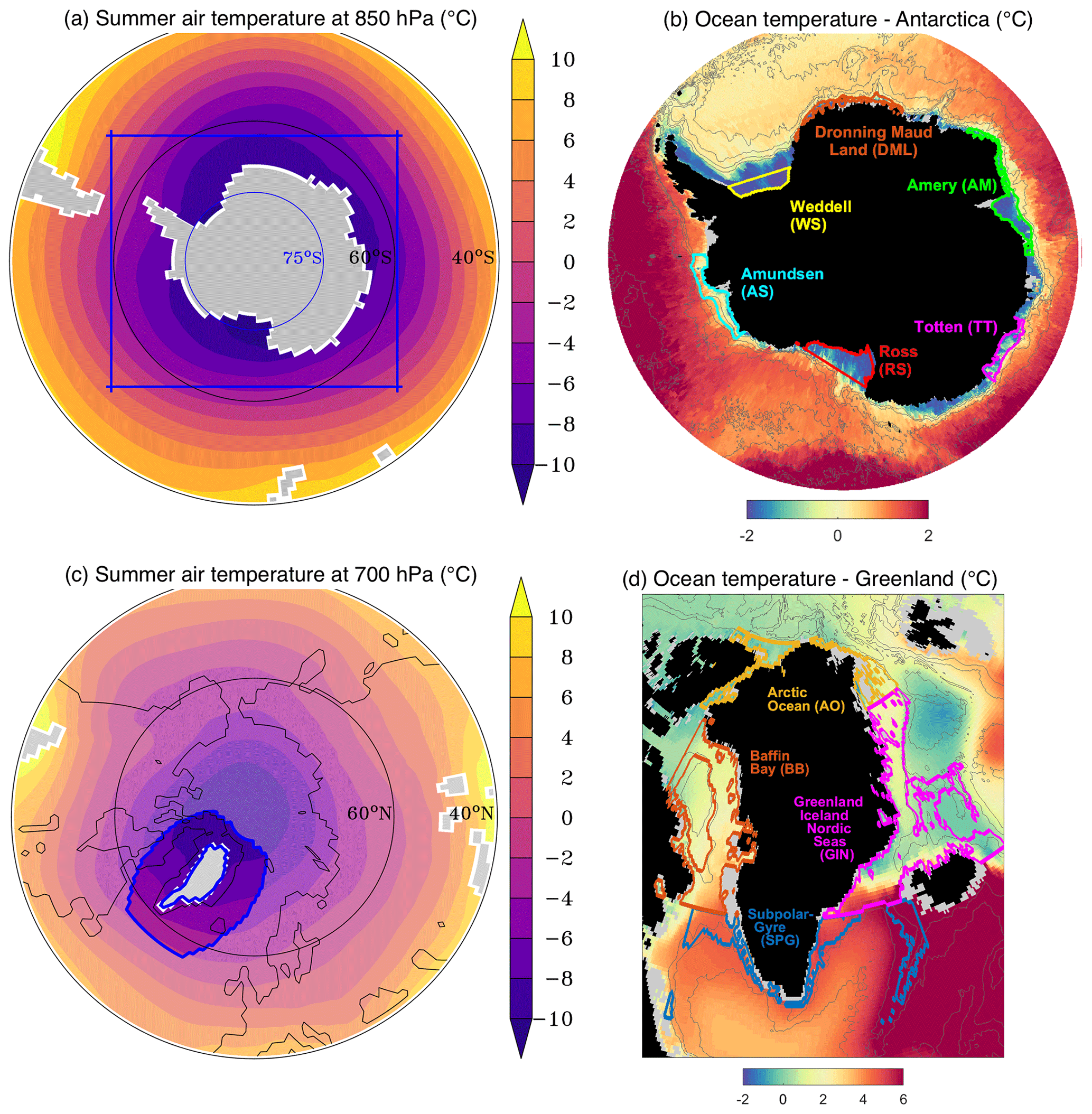
Figure 1Atmosphere and ocean regions defined for metric computation. (a) For Antarctic atmosphere and surface ocean metrics, we considered the domain south of 40∘ S over ocean (color shading). The blue box shows standard lateral boundaries for regional climate models. Color shading is ERA-Interim summer air temperature at 850 hPa over 1980–2004. (b) For Antarctic ocean metrics, we considered six ocean sectors shallower than 1500 m. Color shading shows the depth-integrated temperature of our reference historical climatology. (c) For Greenland atmosphere metrics, we considered the domain inside the usual boundaries of MAR simulations in that region, i.e., inside the blue box, except where ice sheet topography is above 2000 m a.s.l. (bright color shading). Color shading is ERA-Interim summer air temperature at 700 hPa over 1980–2004. (d) For Greenland ocean metrics, we considered the four sectors shown with different colored outlines. Color shading shows the depth-integrated (200 to 500 m) temperature of our reference historical climatology.
Subsurface ocean metrics
The ISMIP6 stand-alone ice sheet oceanic forcing is derived from “far-field” salinity and potential temperature (Slater et al., 2019; Jourdain et al., 2019). Consistent with this approach, our evaluation of subsurface ocean properties is performed on regionally averaged CMIP5 temperatures. Since the oceans around Greenland and Antarctica are characterized by different geographic and dynamic regimes in observations (e.g., Straneo et al., 2012; Schmidtko et al., 2014; Thompson et al., 2018) and models (Yin et al., 2011; Little and Urban, 2016; Levermann et al., 2014), individual metrics are obtained for several subregions surrounding both ice sheets (Fig. 1b, d).
For this purpose, 1989–2009 time-mean ocean temperatures from each CMIP5 model are interpolated onto a common tripolar ORCA025 grid (Ferry et al., 2012), which has a quasi-isotropic resolution corresponding to 0.25∘ in latitude, and 75 vertical layers with a thickness ranging from 1 m at the surface to 200 m at the bottom. We use a conservative 3-D interpolation; if some parts of the ORCA025 grid are not covered by the CMIP grid, we extrapolate from the closest neighbor (horizontally above sills, then vertically to fill troughs behind sills). The regridding tools are made available on https://github.com/nicojourdain/SCRIPTS_CMIP5_ANOM_NOW (last access: 29 July 2019, Dutheil et al., 2019). Regionally averaged coastal ocean temperatures are then computed in six sectors around the Antarctic continent (Fig. 1b), which capture different continental shelf and melting regimes. A maximum bottom depth criterion of 1500 m is used, together with an explicit limit for the northern boundaries in the large embayments in the Ross and Weddell seas, to select ORCA025 ocean cells that are located on the continental shelf near the coast. For Greenland, the ocean has been separated into four connected regions based on the major hydrographic regimes surrounding the ice sheet (Fig. 1d), with a similar cutoff beyond 1500 m bottom depth and geographical distance from the ice sheet to select coastal ocean cells near the ice sheet. For each subregion, volume-averaged temperatures below 200 m depth are computed, providing a scalar nearshore subsurface temperature metric. For Antarctica, the full depth range down to 1500 m is included, while for Greenland, the profiles are truncated below 500 m depth to account for shallow continental shelf depths and bottom sills that typically prevent inflows from greater depths toward the marine-terminating glaciers in Greenland fjords (Morlighem et al., 2017).
Regional volume-averaged temperatures are also computed from available observed ocean climatologies, using the same algorithm as for the model output. For Greenland, observational data are taken directly from the annually averaged statistical fields of the 2013 World Ocean Atlas (WOA; Locarnini and Seidov, 2013). For Antarctica, a refined climatology of coastal water masses was constructed by combining the 2018 WOA data (Locarnini et al., 2019) with statistical fields from the EN4 ocean climatology (Good et al., 2013) and publicly available temperature profiles from seals equipped with satellite relay data loggers (Roquet et al., 2018), with further details provided in Nowicki (2019). In both cases, ocean measurements close to the ice sheets are so sparse that all observations are included in the computation of the regional averages, regardless of their acquisition date.
2.2.2 Aggregating historical metrics
In order to aggregate different metrics of varying nature and magnitude, each of the historical metrics described above (denoted as χ below) is normalized with regards to the 33-model multi-model median and interquartile range (IQR). For each model i,
We average the normalized metrics into three realms: atmosphere, surface ocean (for Antarctica), and subsurface ocean. This decision was made to weaken the dependence of the final ranking on the number of variables used for each realm. Normalization of metrics prevents highly variable or large-amplitude metrics from being overly influential in the average (see Fig. A1) while still penalizing extremes. The final aggregated score for each model is obtained by averaging atmosphere and ocean for Greenland and atmosphere, surface ocean, and subsurface ocean for Antarctica. An alternative aggregating method, where all normalized metrics are weighted equally (12 for Antarctica, 7 for Greenland), is presented in Fig. A2 and does not change our conclusions.
2.3 Projected 21C changes
2.3.1 Climate change metrics
For atmospheric and surface ocean variables, climate change metrics are calculated as the difference between the 2070–2100 mean (RCP8.5) and the 1980–2010 mean (historical) value of each variable, spatially averaged over the entire Greenland and Antarctic atmospheric domains (Fig. 1), denoted with the Δ symbol. The only exception is for change in precipitable water, computed as the difference between the 2070–2100 mean (RCP8.5) and the 1980–2010 mean (historical) divided by the 1980–2010 mean value of each variable, then spatially averaged over the atmospheric domain, denoted with the δ symbol, because it follows a lognormal distribution. For the subsurface ocean, we define metrics as the change in volume-averaged regional temperature between the 1989–2009 and 2080–2100 periods. For Antarctica, we consider four metrics for the atmosphere (change in annual air temperature at 850 hPa, Δta850[a]; in annual precipitable water, δprw[a]; and in position and strength of the tropospheric westerly jet, ΔJpos and ΔJstr), two metrics for the surface ocean (change in winter sea ice extent, Δsie[w]; and in summer sea surface temperature, Δtos[s]), and six metrics for change in subsurface ocean temperature (ΔT), one for each of the sectors defined in Sect. 2.2.2. For Greenland, we define two metrics for the atmosphere (change in annual air temperature at 700 hPa, Δta700[a]; and in annual precipitable water, δprw[a]) and four metrics for change in subsurface ocean temperature (ΔT), one for each ocean sector defined in Sect. 2.2.2.
2.3.2 Maximizing diversity of projected 21C changes
To maximize the diversity of future projections covered in a sub-selection of models of size n, we define the ensemble inter-model spread E by combining the pairwise model differences across the climate change metrics defined in Sect. 2.3.1 (12 for Antarctica, six for Greenland). The spread of a three-model ensemble is computed as the following:
with χ the climate change metrics defined in Sect. 2.3.1. The ensemble that maximizes E for a given ensemble size n (n=3 for top three, n=6 for top six) is the one qualified as “most diverse” in its future projections.
In this section, we focus on the model selection for the Antarctic ice sheet, which is based on historical ranking (Sect. 3.1) and projection diversity (Sect. 3.2). The selected models are presented in Sect. 3.3.
3.1 Historical bias ranking
Over the Antarctic domain, the total normalized historical metric ranges between −0.32 (model of the highest fidelity, CanESM2) and 1.50 (model of the lowest fidelity, BMU-ESM), with a median value of 0.13 (Fig. 2a). Figure 2a shows the 33 climate models ranked by their historical metric, together with contributions of the subsurface ocean (blue), atmosphere (orange), and surface ocean (yellow) to the total historical metric.
Models do not perform equally across the three realms. For example, GFDL-CM3 and EC-EARTH perform well in the atmosphere, with atmospheric metrics of −0.22 and −0.21 respectively, amongst the best models, but are ranked as low fidelity (with total bias scores of 0.46 and 0.54) due to their poor performance in ocean subsurface and surface conditions. Conversely, IPSL-CM5B-LR performs well in the subsurface ocean (metric of −0.20) but is penalized by its poor performance in the atmosphere (metric of 2.07) and surface ocean conditions (metric of 1.77).
Models also do not perform equally within each realm, indicating that biases originate due to regional processes for subsurface ocean or variable-specific biases for surface ocean and atmosphere. We provide the per-variable breakdown of the ocean subsurface metric (Fig. 2b) and ocean surface and atmospheric metrics (Fig. 2c). Although this paper cannot address these differences in detail, we highlight a few notable sources of discrepancies between metrics. For example, the subsurface heat in the Weddell Sea region is the largest single contributor to the ocean bias metric in several models (Fig. 2b), including EC-EARTH, MRI-CGM3, and BNU-ESM. The large ocean heat bias would warrant specific studies investigating the model representation of the ocean climatology in that region. Similarly, in the atmosphere, precipitable water is the largest single bias for models such as IPSL-CM5B-LR, INM-CM4, and MRI-CGCM3 and would warrant further investigation to improve model representation of the historical period.
Models that perform better than the median (historical metric<0.13) have reasonable values for all three realms: the worst metric for each realm is lower than 50 % of the IQR away from the ensemble median for that realm (Fig. 2a). This result gives confidence that these models have a good overall performance, rather than compensating biases across realms. Our averaging method was effective in penalizing models that have a low fidelity over an entire realm. For this reason, selecting the top three models in the top half of the 33 models ensures overall good performance of these models in both the ocean and atmosphere.

Figure 2(a) Ranking of models according to total bias (black) over the Antarctic domain, with a breakdown of the ocean (blue), atmosphere (orange), and surface (yellow) contributions. (b) Breakdown of model performance in the ocean over the Antarctic domain. (c) Breakdown of model performance in the atmosphere (orange) and ocean surface (yellow) over the Antarctic domain. Models are ranked according to total bias. Models selected in the top three (core) ensemble are underlined in red with an asterisk, and models in the top six (targeted) ensemble are underlined in yellow with a † symbol.
3.2 Projected changes
All 33 models considered in this study show an increase in air temperature over the Southern Ocean and Antarctic continent between the end of the 21st century and the end of 20th century climatologies (Fig. 3a), with a multi-model mean increase of 2.54 ∘C. Nevertheless, the ensemble shows a spread of transient climate sensitivity, with an atmospheric warming ranging from 1.3 ∘C (GFDL-ESM2G) to 3.6 ∘C (BNU-ESM), with a median of +2.5 ∘C. We highlight the three core (red) and three targeted (yellow) AOGCMs selected in Sect. 3.3, to illustrate the spread that they cover compared to the 33-model ensemble. Although the projected change in air temperature is only one of the variables we use to diagnose projected atmospheric changes, it provides a good representation of projected changes in the atmosphere. Indeed, the changes in annual air temperature are strongly correlated (R2>0.82) to the projected changes in seasonal air temperature and in annual and seasonal precipitable water and strongly anti-correlated to changes in winter sea ice extent (R2=0.70). Projected changes in wind jet strength, as quantified in Bracegirdle et al. (2018), show a weaker negative correlation with air temperature changes, although a decrease in jet strength is generally associated with a decrease in annual sea ice extent (R2=0.46), as noted in Bracegirdle et al. (2018).
Climate models also overwhelmingly project a 21st century increase in ocean temperatures around Antarctica. For example, the 33 models project a warming of the Amundsen shelf (Fig. 3b), ranging from no significant warming (lowest warming, MRI-CGCM3) to +1.10 ∘C (highest warming, IPSL-CM5B-LR), with a median value of +0.45 ∘C. Other regions show a qualitatively similar range of projected changes, with the highest warming (as quantified by the median value of the ensemble) occurring in the Dronning Maud Land (DML), Amery, and Totten regions (DML median: +0.76 ∘C; Amery median: +0.70 ∘C; Totten median: +0.59 ∘C). The lowest projected warming occurs in the Weddell and Ross regions (Weddell median: +0.21 ∘C; Ross median: +0.30 ∘C). The Amundsen region, presented in Fig. 3b, is currently under scrutiny due to ice shelf thinning and accelerating ice discharge in the last decade (Kimura et al., 2017; Mouginot et al., 2014; Barletta et al., 2018), but this region is projected to warm moderately in the future according to the 33-model ensemble (Amundsen median: +0.45 ∘C).
Unlike the atmospheric warming, which is a good proxy for other atmospheric changes, the projected ocean warming in the Amundsen region is only weakly correlated (R2≤0.016) to other ocean regions. Some significant correlation can be found for neighboring regions in East Antarctica, such as between the Dronning Maud Land and Amery regions (R2=0.71) and between the Amery and Totten regions (R2=0.48), but it is low across other regions (R2≤0.25). Projected changes in the ocean are relatively independent across regions (detailed in Fig. B1), which confirms the added value of quantifying regional ocean metrics rather than metrics integrated over all Antarctic shelves.
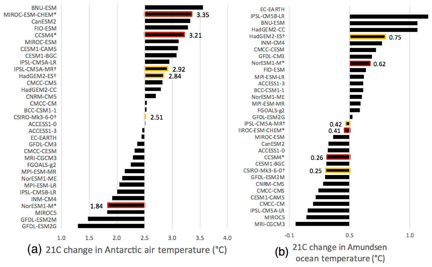
Figure 3Projected RCP8.5 warming for each CMIP5 model in the Antarctic region. (a) Change in 850 hPa air temperature over the Southern Ocean between 1980–2000 and 2080–2100. (b) Change in ocean temperature in the Amundsen region between 1980–2000 and 2080–2100. Models selected in the top three (top six) ensemble are highlighted in red (yellow).
3.3 Recommended ensemble
3.3.1 Top three (core experiments)
In the case of the Antarctic domain, the selection criteria described in Sect. 2 led to six suitable coupled models (CanESM2, NorESM1-M, CSIRO-Mk3-6-0, CCSM4, MIROC-ESM-CHEM, MIROC-ESM), where availability of required data from RCP2.6 projections is the strongest constraint. We then select the three models that maximize the ensemble diversity En=3, as defined in Sect. 2.3.2. The selection is robust to removing one of the metrics at a time and to changing the weight of the metrics in the calculation (Appendix C1).
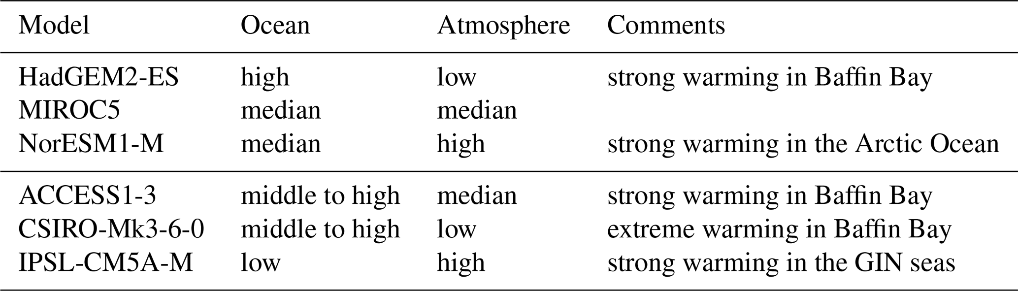
The top three models selected are, in alphabetical order, CCSM4 (pink), MIROC-ESM-CHEM (red), and NorESM1-M (light blue). These three models sample different projected changes in Antarctica under the RCP8.5 scenario (Fig. 4a). Overall, NorESM1-M shows a stronger end-of-21st-century ocean warming than the ensemble median (dashed) but a low atmospheric warming compared to the model ensemble. Conversely, MIROC-ESM-CHEM features an ocean warming similar to that of the ensemble median, associated with strong atmospheric changes, about one IQR higher than the median. Finally, CCSM4 shows very distinct regional patterns of ocean warming, with strong warming in the Weddell and Totten regions and lower warming in the Ross and Dronning Maud Laud regions, relative to the ensemble median. The projected atmospheric changes in CCSM4 are on the high end of the ensemble, qualitatively similar to that of MIROC-ESM-CHEM. The qualitative warming projected by the three models selected for the Antarctic core experiments is summarized in Table 2.
3.3.2 Top six (targeted experiments)
For the additional three models (targeted), CSIRO-Mk3-6-0 (yellow) is chosen because of its good ranking (Fig. 2) and median projected changes (Figs. 3, 4b), and it is preferred to ACCESS1.0 (which also shows median projections under RCP8.5) because of the availability of the RCP2.6 scenario. Each of the metrics of future change lies close to the multi-model ensemble median (see Fig. 4b), meaning that approximately half of the 33 climate models predict higher changes than those of CSIRO-Mk3-6-0, and half predict lower changes.
The other two models selected are, in alphabetical order, HadGEM2-ES (brown) and IPSL-CM5A-MR (dark blue). HadGEM2-ES brings diversity to the six-model ensemble because of its extreme end-of-21st-century warming in the ocean, particularly in the Ross Sea. This extreme regional warming, more than 2 times larger than the IQR from the median value, is ruled out of the top three because it is considered to be a less likely response than those produced by a large number of distinct climate models. Nevertheless, in an intercomparison effort such as ISMIP6, sampling high-end scenarios is essential to (1) examine the response of ice sheet models which may have runaway effects and (2) include high-risk (low probability, high cost) scenarios in terms of future sea level rise. The atmospheric changes produced by HadGEM2-ES are higher than the median, but not outliers. Finally, IPSL-CM5A-MR features an ocean warming lower than the ensemble median in most ocean regions and atmospheric changes higher than the median. It is the only model selected with systematically low warming in the ocean and can be thought of as the converse to NorESM1-M. Robustness of the model selection is demonstrated in Appendix C2. The qualitative warming projected by the additional three models selected for the Antarctic “targeted” experiments is summarized in Table 2.
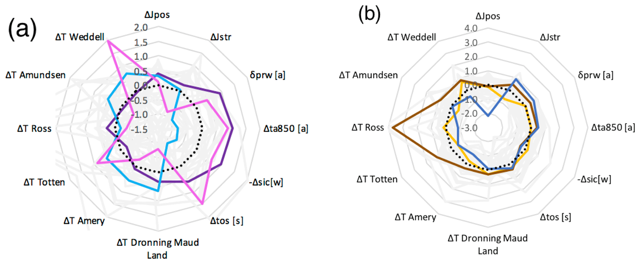
Figure 4Normalized projected 21C changes for Antarctica (with model ensemble in gray and the median in black). (a) Top three: CCSM4 (pink), MIROC-ESM-CHEM (purple), and NorESM1-M (light blue). (b) Top four to six: CSIRO-Mk3-6-0 (yellow), HadGEM2-ES (brown), and IPSL-CM5A-M (dark blue).
In this section, we describe the model selection for the forcing of the Greenland ice sheet. The methods include the model evaluation (Sect. 4.1 and 4.2) and ensemble selection (Sect. 4.3), mirroring the selection performed for the Antarctic ice sheet (Sect. 3).
4.1 Historical bias ranking
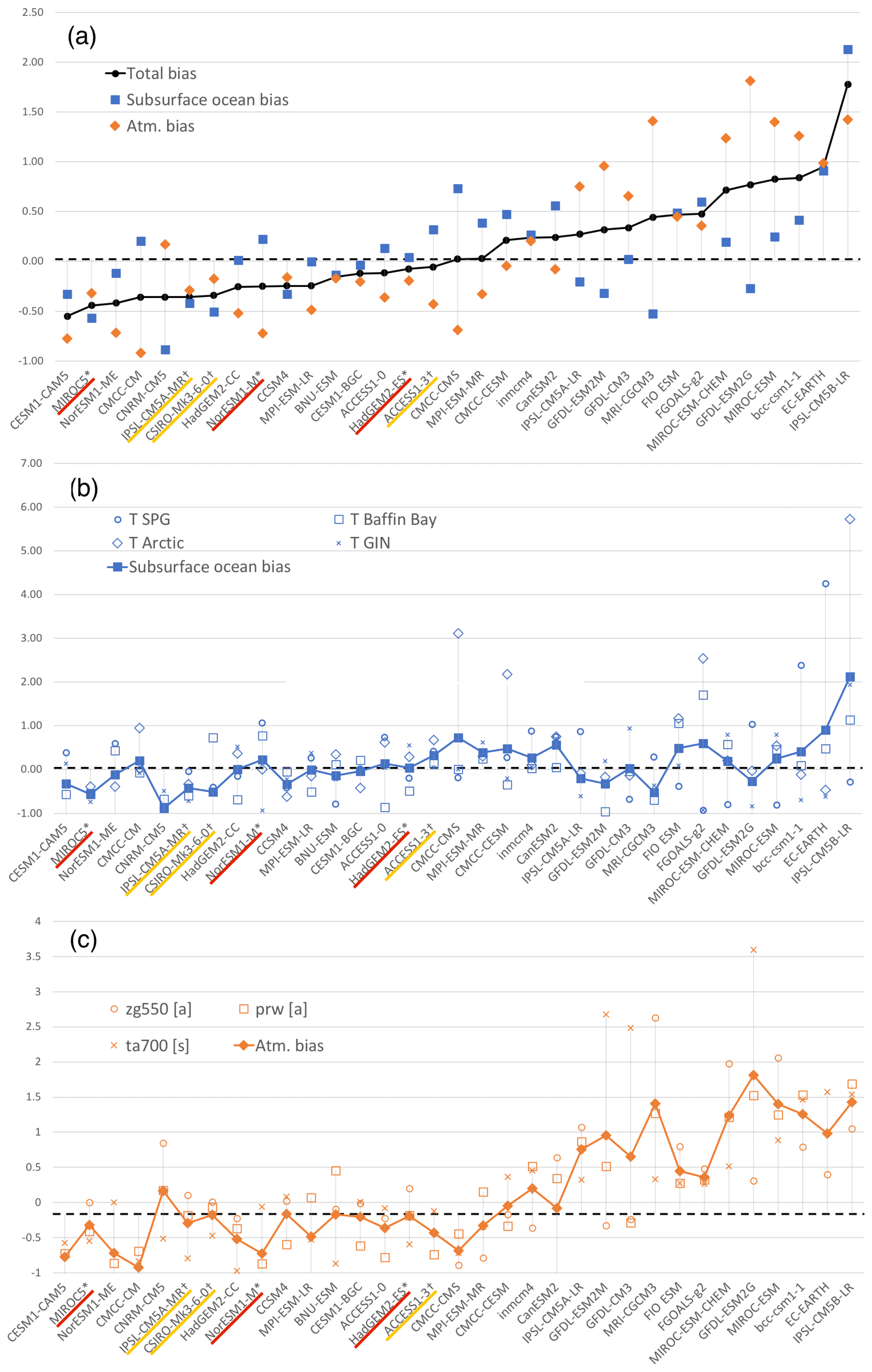
Figure 5(a) Ranking of models according to total bias (black) over the Greenland domain, including the ocean (blue) and atmosphere (orange) contributions. (b) Breakdown of model performance in the ocean over the Greenland domain. (c) Breakdown of model performance in the atmosphere over the Greenland domain. Models are ranked according to total bias. Models selected in the top three (core) ensemble are underlined in red with an asterisk, and models in the top six (targeted) ensemble are underlined in color yellow with a † symbol.
Coupled climate models do not perform equally over the subsurface ocean and the atmosphere (Fig. 5a) around Greenland, consistent with findings for Antarctica, shown in Sect. 3. Some models perform well in the atmosphere but are penalized by their poor ocean performance. For example, CMCC-CMS is the median of the ensemble and features one of the lowest biases in the atmosphere (−0.69) and one of the highest biases in the ocean (0.73). Conversely, others perform well in the ocean but show high biases in the atmosphere (e.g., MRI-CGCM3). This unequal performance across the ocean and atmospheric variables supports the need to assess several components of coupled climate models together, rather than separately.
Investigating the source of biases in any given model is beyond the scope of this paper, which focuses on selecting six models suitable for the ISMIP6 simulations. Nevertheless, the ranking of the models can highlight significant biases. For example, the ocean bias in several models, most notably CMCC-CS, CMCC-CESM, and IPSL-CM5B-LR, is dominated by a bias in ocean heat in the Arctic region. This large bias in temperature would warrant a specific study to improve model representation of that region. However, the observations in this region are scarce and we have a lower degree of confidence in the resulting ocean climatology in that region than in more frequently and densely observed regions, as discussed in Sect. 5.
The model ranking around Greenland highlights that the fidelity of coupled models is regionally dependent. The models of the highest fidelity around Greenland do not necessarily perform well around Antarctica and vice versa. For example, CanESM2 is the best-ranked model for Antarctica (see Sect. 3) but is ranked in the lower half of the ensemble around Greenland due in part to its ocean biases. Likewise, MIROC5 performs well on all metrics around Greenland, and has been extensively used in the relevant literature (e.g., Fettweis et al., 2013; Tedesco and Fettweis, 2012), but has strong atmospheric biases over Antarctica. Climate models are not expected to perform equally in all regions; nevertheless, it is important for the scientific community to keep those regional variations in mind, especially if using existing studies performed over a different region. This unequal performance across the Greenland and Antarctic regions also supports our decision to perform model ranking and selection independently for the two ice sheets.
Finally, the models that perform better than the median have ocean and atmosphere biases that lie lower than 0.5 IQR away from the median. Although biases in individual (regional) variables may be higher than that, this result confirms that the best-ranked models have a good performance in both the subsurface ocean and the atmosphere and gives us confidence that the top half of the ensemble models are suitable candidates for the Greenland model selection.
4.2 Future projection diversity
All 33 AOGCMs project atmospheric warming over Greenland by the end of the 21st century. Projections range from +1.95 ∘C (lowest warming, FIO-ESM) to +5.95 ∘C (highest warming, MIROC-ESM-CHEM) with a median warming of +4.09 ∘C (Fig. 6a). Models that made our final selection, highlighted in red (top three) and yellow (top six), sample a range of future warming. Similar to results presented for Antarctica (Sect. 3), the changes in annual air temperature over Greenland are a good proxy for most other atmospheric changes. Increase in 700 hPa air temperature is associated with an increase in precipitable water (R2=0.96), an increase in ocean surface temperature (R2=0.60), and a decrease in summer sea ice cover (R2=0.29).
Most models also project an increase in ocean temperature on the shelf surrounding Greenland. Baffin Bay, for example, is projected to warm by +0.48 ∘C by the end of the 21st century, with models projecting between +0.07 ∘C (lowest warming, BCC-CSM1-1) and +1.70 ∘C (highest warming, CanESM2). The models selected in Sect. 4.3, highlighted in Fig. 6b, cover a range of projected warming in Baffin Bay. Two other regions show similar projected changes (Arctic median: +0.48 ∘C; Subpolar Gyre (SPG) median: +0.49 ∘C). The highest projected warming occurs in the Greenland–Iceland–Norwegian region (GIN), with a median warming of +0.76 ∘C.
Projected changes across the ocean regions are correlated between the Arctic Ocean and GIN regions (R2=0.58) and mildly correlated between the SPG and GIN regions (R2=0.31). Other regions are only weakly correlated with each other (detailed in Fig. B2), and ocean changes show no significant correlation with the projected atmospheric changes (R2<0.06).
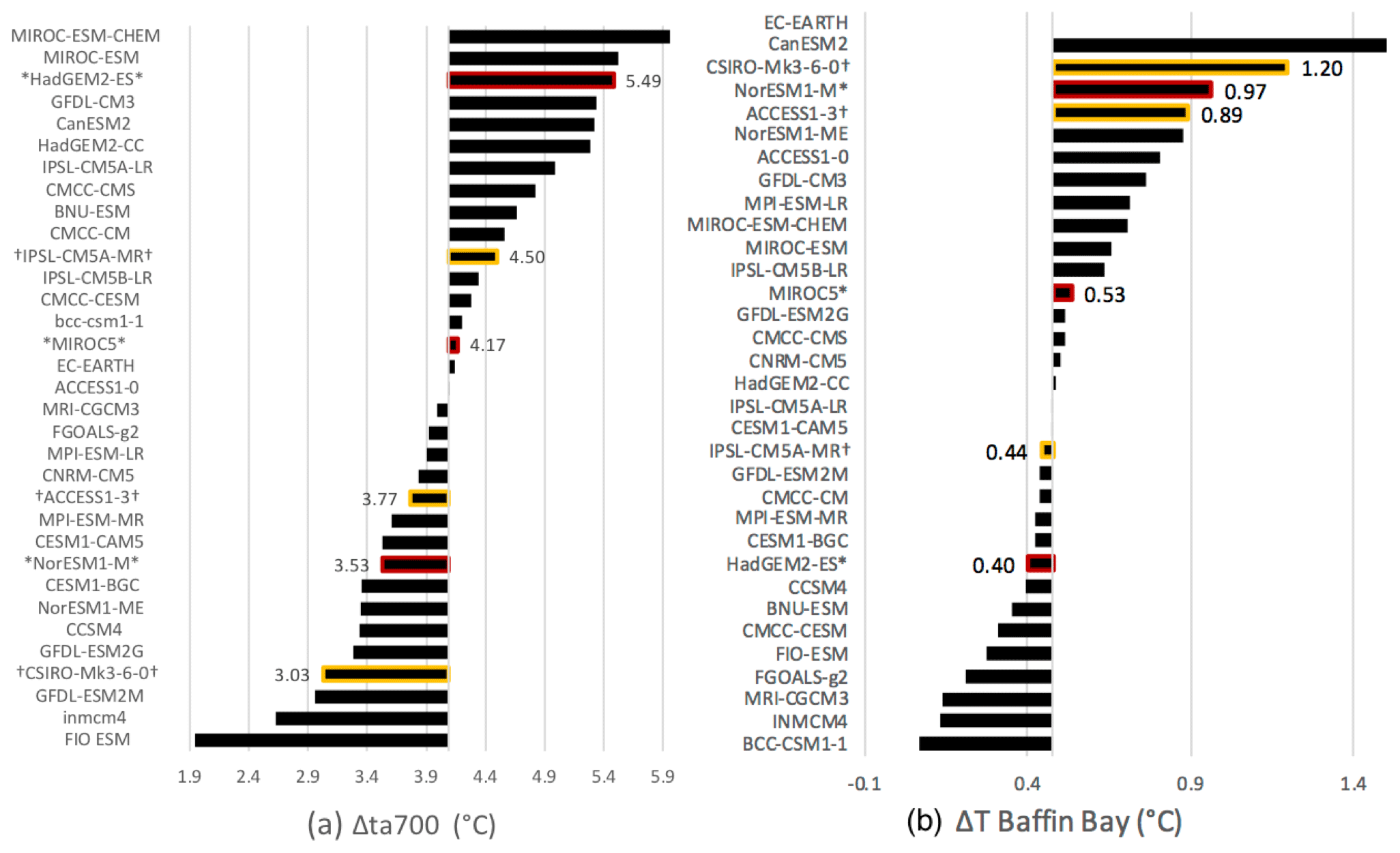
Figure 6Projected RCP8.5 warming for each CMIP5 model over Greenland. (a) Change in 700 hPa air temperature over the Southern Ocean between 1980–2000 and 2080–2100. (b) Change in ocean temperature in the Baffin Bay region between 1980–2000 and 2080–2100. Models selected in the top three (top six) ensemble are highlighted in red (yellow).
4.3 Recommended ensemble
In the case of Greenland, the availability of sub-daily outputs is a strong constraint for the model selection. This was a determining factor because existing studies over Greenland show that RCMs outperform global climate models in representing realistic surface mass balance (e.g., Noël et al., 2018; Fettweis et al., 2013).
4.3.1 Top three (core experiments)
When applying the selection criteria described in Sect. 2 and removing CNRM-CM5 and EC-EARTH due to unavailable data, six models remain for the top three selection (MIROC5, IPSL-CM5A-MR, NorESM1-M, ACCESS1-0, ACCESS1-3, HadGEM2-ES). In this case, MIROC5 was preselected, as it features changes similar to those of the ensemble median (dotted; Fig. 7a), meaning half of the models project stronger changes than those of MIROC5, and half project weaker changes. Two additional models are selected, maximizing ensemble diversity of three models (MIROC5, model 1, model 2). The top three models selected are, in alphabetical order, HadGEM2-ES, MIROC5, and NorESM1-M. These three models show different patterns of projected changes by the end of the 21st century (Fig. 7a). As described above, MIROC5 is chosen as a good representation of the overall ensemble. HadGEM2-ES features high atmospheric changes, including increases in air temperature and precipitable water, of a magnitude stronger than the ensemble median. The projected changes in ocean heat are more regionally dependent, with warming higher in the Arctic and GIN (northeast) and lower in Baffin Bay and SPG (southwest) relative to the ensemble median. Conversely, NorESM1-M features a warming in the atmosphere on the low end of the 33-model ensemble projections. The ocean warming is also regionally dependent, with NorESM1-M featuring low warming in GIN, the Arctic, and the SPG regions and a strong warming in the Baffin Bay region. The qualitative warming projected by the three models selected for the Greenland core experiments is summarized in Table 3.
4.3.2 Top six (models for the targeted experiments)
For the top six selection, five models (IPSL-CM5A-MR, CSIRO-Mk3-6-0, CCSM4, ACCESS1-0, ACCESS1-3) are available to complement the already selected top three.
The selected models are, in alphabetical order, ACCESS1-3, CSIRO-Mk3-6-0, and IPSL-CM5A-MR. CSIRO-Mk3-6-0 projects a low atmospheric warming, far below the median value, alongside an extreme warming in the southwest ocean regions (ΔT BB>2; ΔT SPG=0.94). ACCESS1-3 adds diversity to the ensemble as it shows strong warming in Baffin Bay and the Arctic Ocean but low warming in the Subpolar Gyre (SPG) region. Its atmospheric warming is close to the median. Finally, IPSL-CM5A-MR project strong warming in the Greenland–Iceland–Norwegian seas (GIN), while other ocean regions and atmospheric variables are closer to the median. The qualitative warming projected by the additional three models selected as forcing for the Greenland targeted experiments is summarized in Table 3.
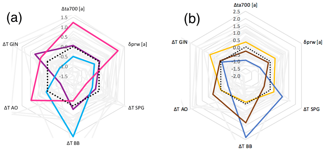
Figure 7Normalized projected 21C changes for Greenland (with model ensemble in gray and the median in black). (a) Top three: HadGEM2-ES (pink), MIROC5 (purple), and NorESM1-M (light blue). (b) Top four to six: ACCESS1-3 (brown), CSIRO-Mk3-6-0 (dark blue), and IPSL-CM5A-MR (yellow). Ocean warming is calculated over four sectors (BB: Baffin Bay; AO: Arctic Ocean; GIN: Greenland–Iceland–Norwegian seas; SPG: Subpolar Gyre).
In this study, we evaluated the performance of 33 CMIP5 AOGCMs relative to reanalyses and gridded observational datasets covering the atmosphere, sea surface, and subsurface ocean around the Greenland and Antarctic ice sheets. We also assessed 21st century changes in key oceanic and atmospheric variables. Time constraints for ISMIP6 simulations drove several decisions relating to the scope of this analysis, including the use of the CMIP5 (rather than the now partially available CMIP6) ensemble, the use of AOGCMs that had already been processed and regridded for both the ocean and atmosphere, and the use of available observational products with limitations and biases, particularly in the ocean subsurface. However, this assessment of near-ice-sheet present-day and future climate remains the most comprehensive performed to date.
Many subjective choices were made in the model selection process. We have attempted to document these choices, and note that the relative insensitivity of results to alternate choices (e.g., Fig. A.2, Appendix C) provides some confidence that our rankings are robust for the CMIP5 ensemble. However, because the evaluation and selection exercise will have to be repeated for future model ensembles (e.g., CMIP6), our discussion focuses on key elements of our methodology that could be further developed. Implications are discussed with respect to results from the full 33-member ensemble to extend the relevance to other exercises where the small ensemble required for ISMIP6 may not apply.
Model selection was made largely based on their representation of the present-day local climate, with the implicit assumption that biases relative to observations reflect a poor representation of processes of relevance to future warming. It is difficult to determine whether performance relative to this set of present-day regional metrics is (1) a sufficient means to evaluate AOGCMs and (2) relevant to the rate of 21st century near-ice-sheet warming. Krinner and Flanner (2018) show that model biases are stationary under future climate change within the CMIP5 dataset, providing justification for using less biased models for climate change studies. However, over the long timescales that ISMIP6 seeks to assess, different processes and/or biases (global and/or nonlocal ocean warming rates, e.g., stratospheric ozone recovery) may be equally important; i.e., even if a model closely matches historical conditions, key processes for projections may still be missing.
Support for the relevance of these metrics might be derived from a clear relationship between the modern state and projections of change across models (so-called “emergent constraints”). Bracegirdle et al. (2015) and Agosta et al. (2015) found that 21st century changes in Antarctic air temperature and precipitation rate (and, perhaps surprisingly, jet strength; Bracegirdle et al., 2018) were correlated to sea ice area bias across models. In this analysis, we found no significant correlation between historical biases and climate changes over Antarctica (or Greenland). A plausible explanation is our use of an 850 hPa (rather than surface) temperature metric and our circum-Antarctic study region. However, this result may also indicate a sensitivity to the specific models included in the ensemble: we find that the magnitude and significance of inter-model correlations are sensitive to whether all or a set of the best-performing models are assessed. Shared code and parameterizations across models may also underlie some of the modest correlations evidenced in our analysis.
It is difficult to determine whether the historical metrics chosen in this analysis are comprehensive (e.g., account for all relevant processes) and/or independent. Concerning independence, we eliminated metrics which represent the same physical processes and are strongly correlated (e.g., the precipitation and air temperature variables in Bracegirdle et al. (2015) are strongly correlated to those in Agosta et al. (2015) and were not included in this study). Assessing comprehensiveness is more difficult. For example, the choice of metrics is constrained by the availability of observations. In particular, oceanographic measurements in the vicinity of ice sheets are very sparse and feature sharp horizontal gradients in water masses (e.g., Thompson et al., 2018). As a result, we chose to calculate volume- and time-mean quantities over subjectively defined regions in order to maximize the number of observations included. It is unclear which ocean region is most “important” in terms of future mass balance. The optimal number of regions, based on their relevance to future ice sheet change and their independence, remains to be determined. These choices should be expected to influence evaluations of both performance and warming. In contrast, observations for the atmosphere and surface ocean have better spatiotemporal coverage. Correspondingly, the metrics chosen were continental scale and seasonally resolved. However, our continental-scale evaluation may obscure regional variability. Atmospheric dynamical modes, such as variability in the Amundsen Sea Low and the Southern Annular Mode (SAM), strongly impact the regional climate in Antarctica (Holland et al., 2017; Fyke et al., 2017). Although our grid-point error metric reflects biases in atmospheric pressure, it is not able to attribute the bias to a model's lack of fidelity to, say, the asymmetric nature of the SAM. Future work should more formally assess the number and relative weighting of regional metrics in the atmosphere and ocean and include dynamically relevant measures of asymmetry. Similar concerns apply to the metrics of future warming and their relevance to ice sheet mass balance. We note that our analysis does not address the rate of warming, which differs widely across models. In the ocean, the rate and timing of warming may have dramatic effects on 21st century ice sheet evolution (Hellmer et al., 2012; Timmermann and Goeller, 2017).
We have noted the unequal performance of coupled climate models over different realms, which we suggest highlights the importance of assessing model fidelity over a range of metrics combining the subsurface ocean, surface ocean, and atmosphere conditions. It also explains why the present ranking of models differs from existing intercomparison studies specifically focused on the atmosphere (e.g., Agosta et al., 2015) or the ocean (e.g., Meijers et al., 2012; Sallée et al., 2013; Russell et al., 2018). For example, the metrics used in Agosta et al. (2015) led to EC-EARTH and CanESM2 being ranked closely (8 and 9 out of 41 models), implying similar performance. However, by including the subsurface ocean metrics, our results point to CanESM2 as the model with the best fidelity overall, while EC-EARTH is in the lower half of the 33-model ensemble due to its poor performance in the ocean (other examples of differences in rankings across realms can be found by examining Figs. 2 or 5). As Agosta et al. (2015) focuses purely on the model performance for ice sheet surface mass balance, their results differ from the current study evaluating both the ocean and atmospheric metrics for the sake of providing the atmosphere-driven surface mass balance and the ocean-driven melt from the same coupled model as boundary conditions to ice sheet models. This underscores the importance of considering the original aim of an intercomparison, including the variables and the regions considered, before interpreting or applying a ranking derived from the analysis.
Antarctica and Greenland were treated independently, supported by the different model performance across the ensemble. A different set of models was selected for Greenland and Antarctica, suggesting model performance varies in polar regions of different hemispheres. However, with respect to future warming, it is reasonable to expect some degree of interhemispheric correlation in warming (e.g., due to a high AOGCM climate sensitivity). It is unclear how this inter-ice-sheet independence assumption could influence sea level projections, as it depends upon the response of surface mass balance (SMB) and changes in ice flux of the different ice sheets.
Using aggregated measures of present-day performance and future climate changes, we selected six AOGCMs as adequate and representative of future near-ice-sheet warming pathways. This ensemble size was judged to be reasonable for ISMIP6, given computational limitations and the goal to sample different sources of uncertainty (e.g., model, RCP scenarios, parameterizations, parameters values). However, given the many degrees of freedom across the evaluation metrics, it is difficult to select a fully representative sample. Some limitations of the sample size are apparent, notably the nonuniform distribution across parameters (e.g., no low ocean warming sampled). Furthermore, the models selected are not structurally independent. For example, HadGEM2-ES and ACCESS1-3 share a common Hadley Centre atmospheric model, while NorESM1 and CCSM4 share the NCAR Community Atmospheric Model. Such interdependence may limit the diversity of forcing applied to ISMIP6 models. We do note that even if ISMIP6 had the ability to evaluate all available CMIP5 AOGCMs, issues with statistical sampling and diversity of CMIP models, code similarities/independence, and quality would persist (Knutti et al., 2013; Sanderson et al., 2015a, b). Future model evaluation studies may invert the process used here, i.e., objectively assess the appropriate number of models to achieve sufficient diversity in forcing.
Finally, we emphasize that evaluation is only a first step to a better process-based understanding of the differences between models. It is critical to assess the processes that make models (or model families) perform better or project climate warming at different rates. We invite modeling groups or researchers interested in examining these to trace back the source of the bias in individual models or across the larger ensemble.
Table 2Selected AOGCMs for Antarctica and their qualitative projected warming.
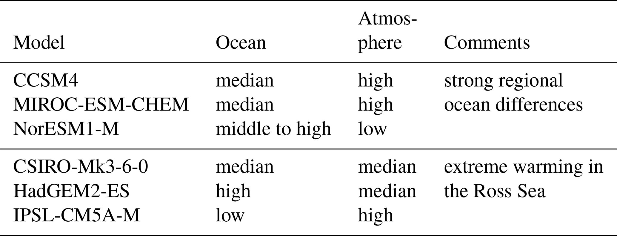
Table 3Selected AOGCMs for Greenland and their qualitative projected warming.
As part of the Ice Sheet Model Intercomparison Project for CMIP6 (ISMIP6), ice sheet models will be forced with climate model-derived time series of basal melt (for Antarctica), front retreat (for Greenland), and surface mass balance. To generate such forcing, a subset of CMIP5 models has been selected according to (i) their realistic representation of the historical period (compared to reanalysis data) and (ii) the diversity of the projected 21st century changes under RCP8.5 within the selected subset. As a result of the evaluation and selection process performed in this study, six AOGCMs have been selected for ISMIP6 Antarctic future projection runs, including three for the core experiments (CCSM4; MIROC-ESM-CHEM; NorESM1-M) and three for the additional targeted experiments (CSIRO-Mk3-6-0; HadGEM2-ES; IPSL-CM5A-M) (see Table 2). Independently, six AOGCMs have been selected for ISMIP6 Greenland future projection runs (core experiments: HadGEM2-ES, MIROC5, NorESM1-M; targeted experiments: ACCESS1-3, CSIRO-Mk3-6-0, IPSL-CM5A-M; see Table 3). Ocean and atmospheric data from these AOGCMs are used to generate ice sheet surface mass balance, the Greenland retreat parameterization (e.g., Slater et al., 2019), and the Antarctic basal melt parameterization (Nowicki, 2019), which will be presented in detail in upcoming papers. It is expected that the range of near-ice-sheet climate changes simulated by these AOGCMs will result in diverse projections of ice sheet mass balance change when used to force ISMIP6 simulations. The evaluation and selection of models was a necessary first step to develop the current ISMIP6 experiment protocol and can be improved upon for the next phase of ISMIP in multiple ways. Firstly, future studies will evaluate and select models from the CMIP6 ensemble. Repeating this study with CMIP6 data will provide insight into whether new developments in climate models reduce ocean and atmospheric biases near ice sheets. Secondly, results from the ice sheet simulations will provide insight into ice sheet model sensitivity. For example, future model selection may weight atmospheric changes more heavily than ocean changes if ice sheet models show a higher sensitivity to surface mass balance. In addition, future selection should look to include more dynamical metrics (e.g., Amundsen Sea Low representation, ocean slope front position) and consider the rate of projected changes in the ensemble diversity. These improvements will ensure that, in an intercomparison project that remains computationally limited, we prioritize the forcing that is most fruitful.
Appendix A provides additional information illustrating the robustness of the historical ranking methodology.
Firstly, we demonstrate the need to normalize the historical bias metrics (Fig. A1). As the atmospheric bias metrics are based on variables as distinct as temperature, pressure, sea ice extent, and precipitable water, the raw bias metrics have different mean values and different inter-model variability (Fig. A1a). By normalizing each metric by its ensemble median and interquartile range, the (normalized) metrics are scaled to cover a similar inter-model variability (Fig. A1b) and can be combined into a single metric independently of the original magnitude of the raw variable.
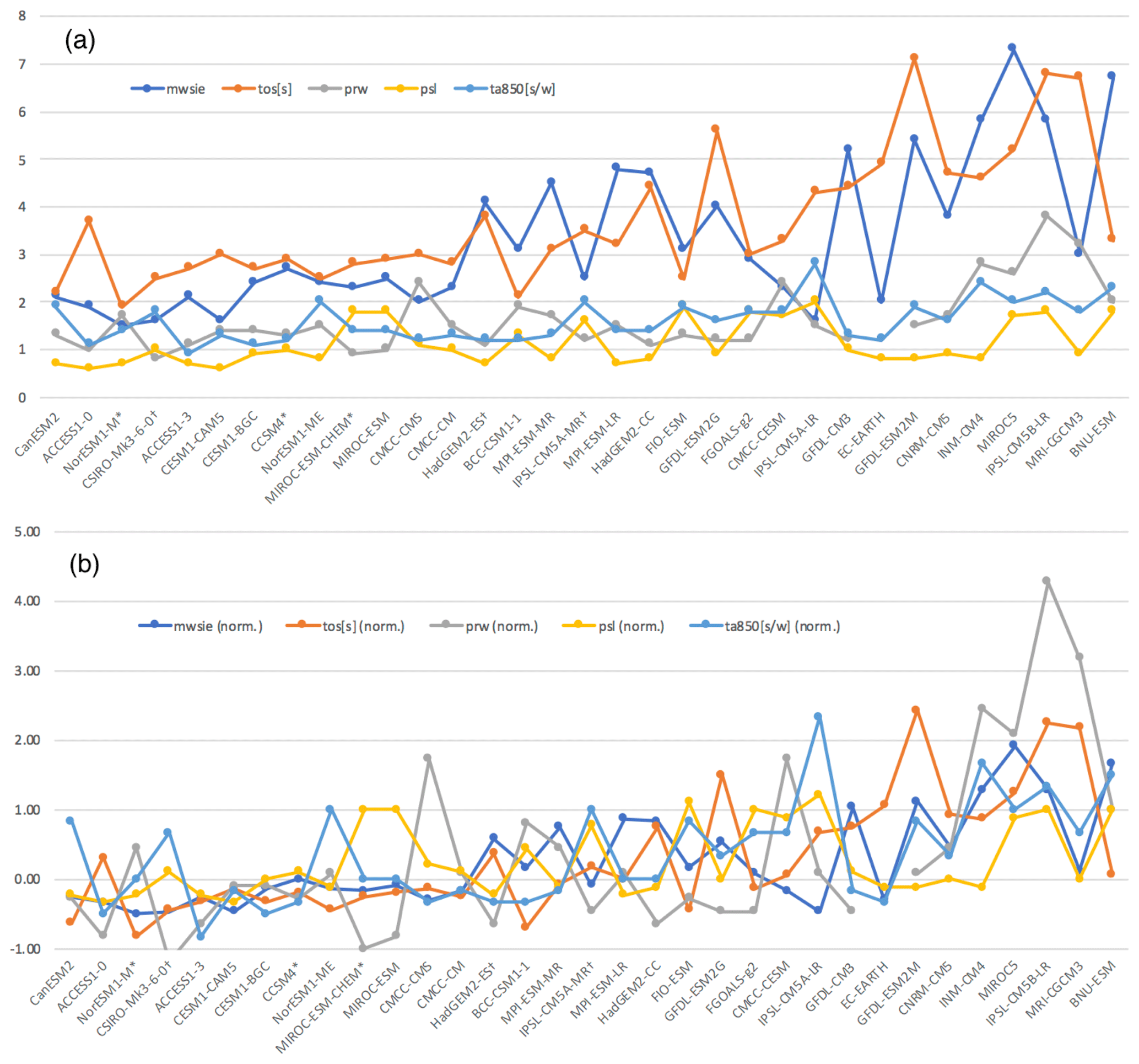
Figure A1Normalization of variables. (a) Historical atmospheric biases for the Antarctic domain; (b) normalized historical atmospheric biases for the Antarctic domain. The non-normalized variables have different mean values and different variability. The normalization removes the offset and rescales the variability, so that variables of different nature, magnitude, and variability can be combined into one atmospheric bias metric. The * and † symbols identify models selected in the top three and top six ensembles, respectively.
Secondly, we illustrate the robustness of the historical ranking to the averaging method by providing an alternate ranking. In Fig. A2, the AOGCMs are ranked by averaging all (normalized) bias metrics with equal weight (dashed), instead of the bias metric used in this study (where each realm is given the same weight; black). For both the Antarctic (Fig. A2a) and Greenland (Fig. A2b) domains, the difference in ranking is minor, as only two models would switch between the top and bottom 50 % of the 33-model ensemble, and neither of these models is present in the top three or top six ensembles.
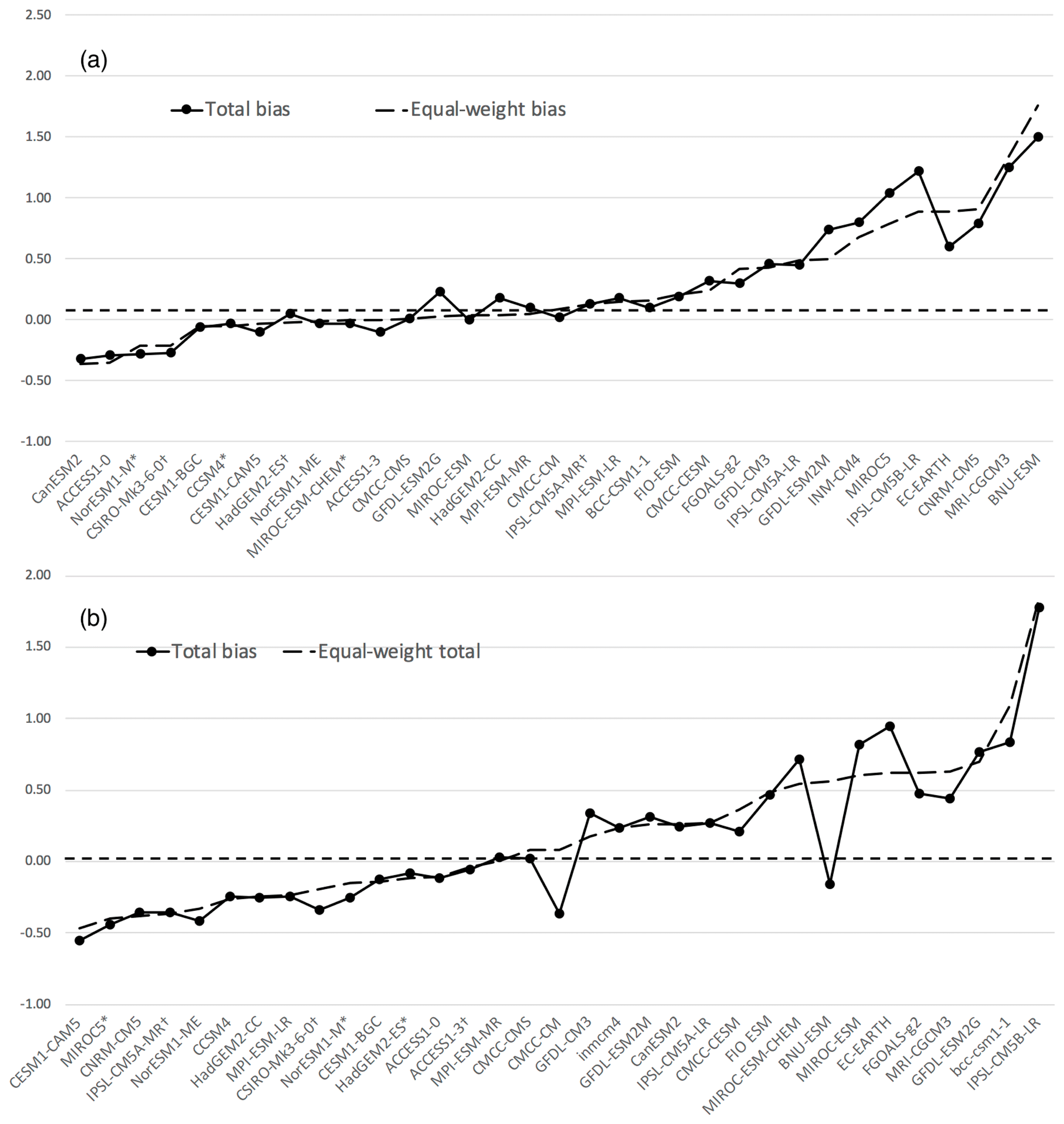
Figure A2Alternate ranking of AOGCMs according to an equal-weight total bias (dashed black) compared to the realm-averaged total bias (black) over (a) the Antarctic domain and (b) the Greenland domain. The symbols * and † identify models selected in the top three and top six ensembles, respectively.
Appendix B presents details of the projected ocean warming for each CMIP5 model between 1980–2000 and 2080–2100 under the RCP8.5 scenario. The warming over the six Antarctic shelf regions is presented in Fig. B1, while the warming over the four Greenland shelf regions is presented in Fig. B2. In each region, labels and markers (*,†) identify models selected in the top three and top six ensembles, respectively. In each region, the majority of AOGCMs predict a warming by the end of the 21st century, although the magnitude and inter-model spread of warming is regionally dependent.
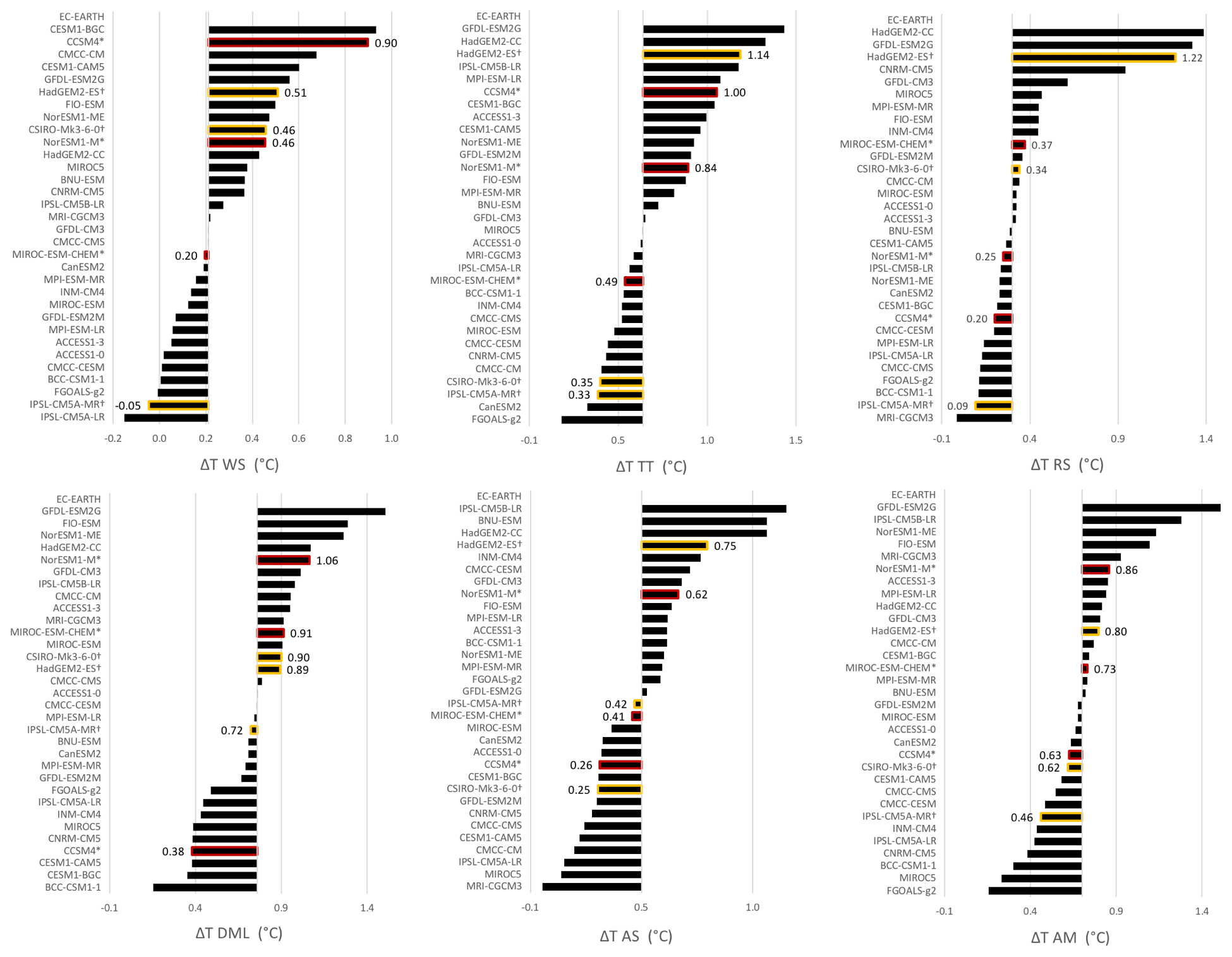
Figure B1Projected RCP8.5 warming for each CMIP5 model between 1980–2000 and 2080–2100 in the six Antarctic shelf regions (WS: Weddell Sea; TT: Totten; RS: Ross; DML: Dronning Maud Land; AS: Amundsen; AM: Amery). The symbols * and † identify models selected in the top three and top six ensembles, respectively.
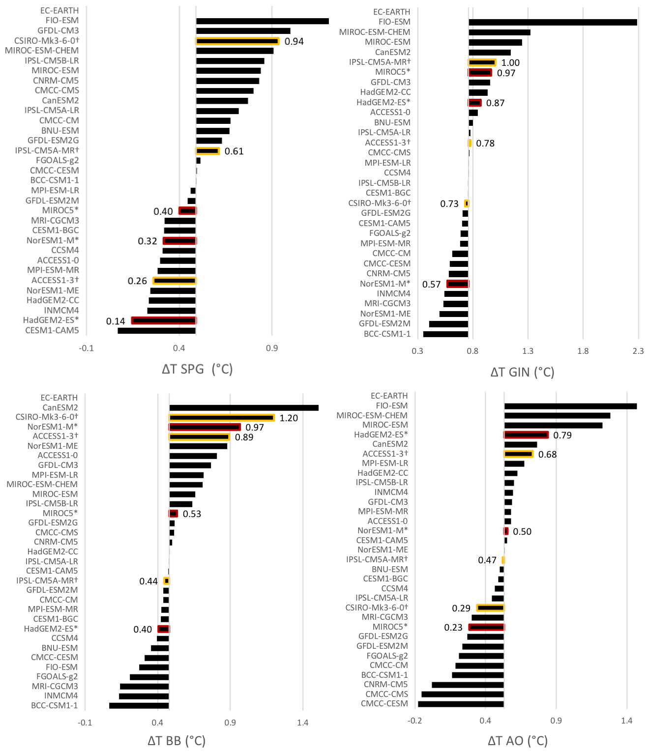
Figure B2Projected RCP8.5 warming for each CMIP5 model between 1980–2000 and 2080–2100 in the four Greenland shelf regions (SPG: Subpolar Gyre; GIN: Greenland–Iceland–Norwegian seas; BB: Baffin Bay; AO: Arctic Ocean). The symbols * and † identify models selected in the top three and top six ensembles, respectively.
This appendix describes robustness of the model selection to modifications of the choice and weight of metrics. We repeat the model selection for the top three and top six models for Antarctica (Sect. 3.3) and Greenland (Sect. 4.3) under removal of one of the metrics at a time and under a change of the weighting. Overall, the model selection is robust to the described modifications.
C1 Robustness of Antarctic model selection top three
Table C1 lists the selected model combinations with absolute and relative frequency of occurrence for the Antarctic top three model selection. The final model combination (NorESM1-M, MIROC-ESM-CHEM, CCSM4) occurs in 9 of 12 cases. One additional model (CanESM2) is selected in 25 % of the cases. Table C2 lists the absolute and relative occurrence of each individual model in the possible combinations presented in Table C1.
Table C1Possible model combinations for the Antarctica top three selection, with absolute and relative frequency of occurrence when applying the robustness test.

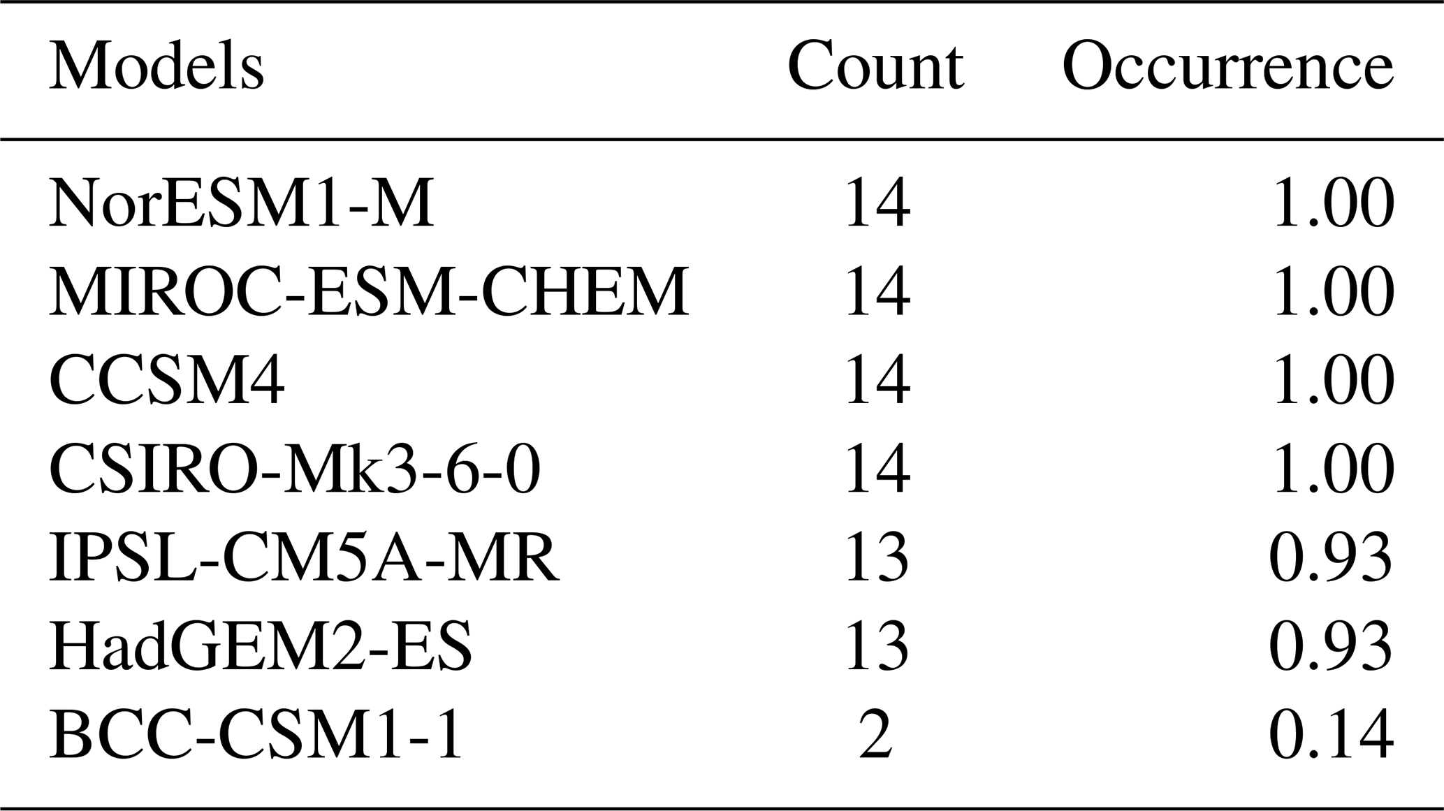
Table C2Absolute and relative occurrence of each individual model included in the Antarctica top three combinations presented in Table C1.

C2 Robustness of Antarctic model selection top six
Table C3 lists the selected model combinations with absolute and relative frequency of occurrence for the Antarctic top six selection. The final model combination (NorESM1-M, MIROC-ESM-CHEM, CCSM4, CSIRO-Mk3-6-0, HadGEM2-ES, IPSL-CM5A-MR) occurs in 12 of 14 cases. Table C4 lists the absolute and relative occurrence of each individual model in the combinations given in Table C3. When equal weighting of the 14 metrics is applied, giving more emphasis on the surface ocean, HadGEM2-ES is still selected in 4 of 14 cases, but replaced by MPI-ESM-MR in the majority of cases (9 of 14).
Table C3Possible model combinations for the Antarctica top six selection, with absolute and relative frequency of occurrence when applying the robustness test.
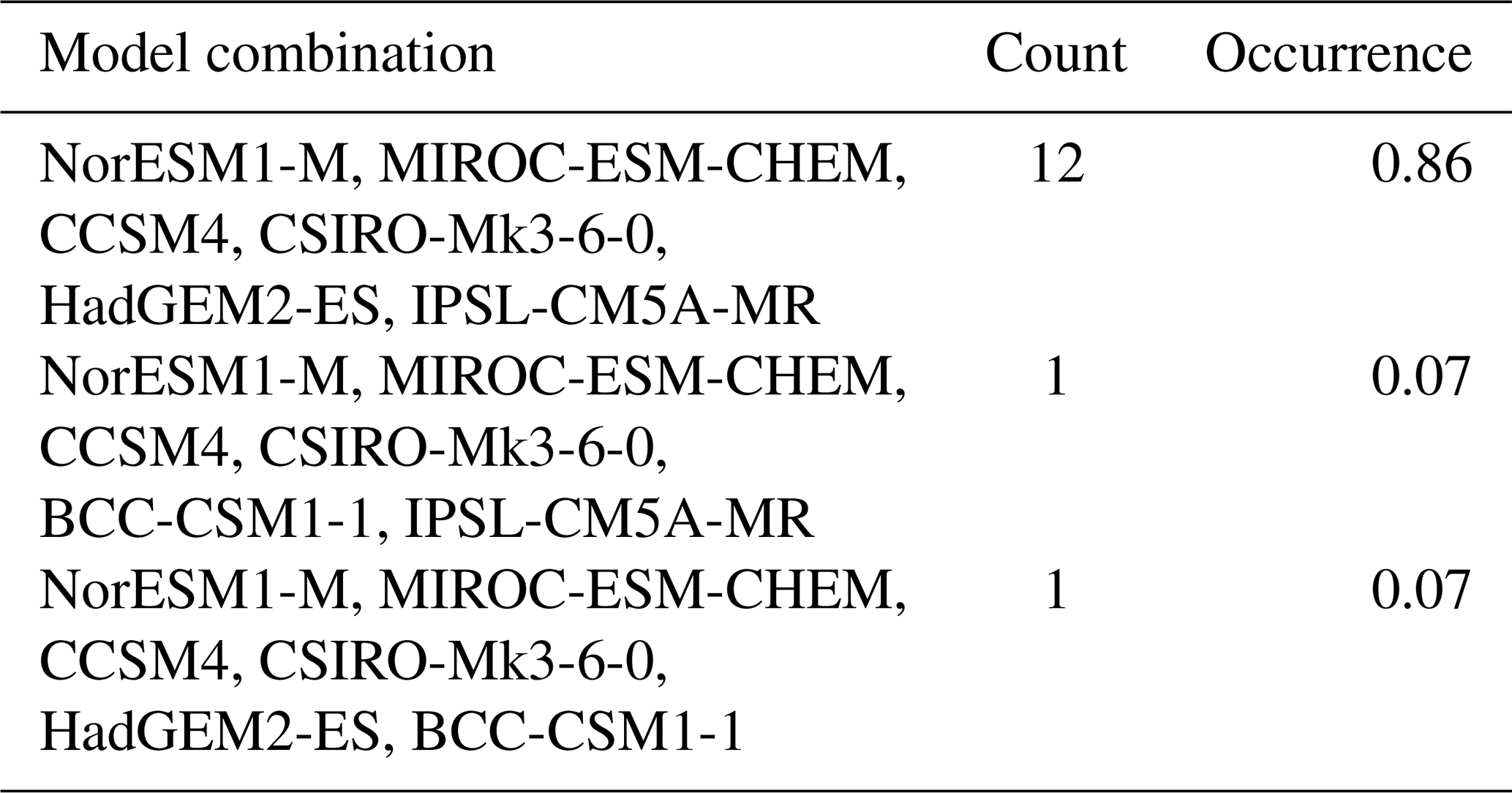
Table C4Absolute and relative occurrence of each individual model included in the Antarctica top three combinations presented in Table C3.
C3 Robustness of Greenland model selection top three
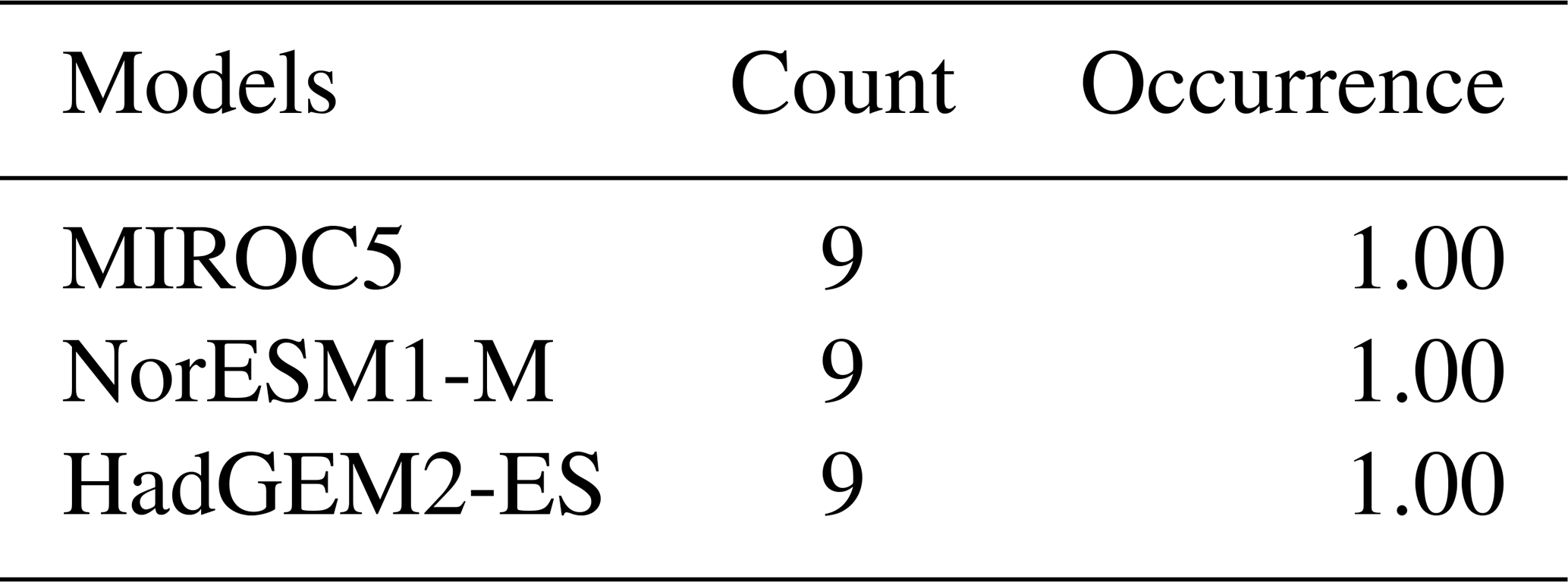
Table C5 lists the selected model combinations with absolute and relative frequency of occurrence for the Greenland top three selection. The final model combination (MIROC5, NorESM1-M, HadGEM2-ES) was selected in all cases. Table C6 lists the absolute and relative occurrence of each individual model in the combinations given in Table C5.
The same results were obtained when metrics for the surface ocean (Δsst [a], Δsie [s], Δsie [w]) were added to the other metrics (Δ700 hPa [a], δprw [a], ΔT SPG, ΔT BB, ΔT AO, ΔT GIN).
Table C5Possible model combinations for the Greenland top three selection, with absolute and relative frequency of occurrence when applying the robustness test.
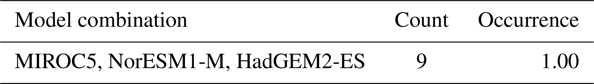
Table C6Absolute and relative occurrence of each individual model included in the Greenland top three combinations presented in Table C5.
C4 Robustness of Greenland model selection top six
Table C7 lists the selected model combinations with absolute and relative frequency of occurrence for the Greenland top six selection. The final model combination (MIROC5, IPSL-CM5A-MR, CSIRO-Mk3-6-0, NorESM1-M, HadGEM2-ES, ACCESS1-3) occurs in seven of nine cases, with CCSM4 replacing ACCESS1-3 in the remaining two cases. Table C8 lists the absolute and relative occurrence of each individual model in the combinations given in Table C7. Similar results were obtained whether metrics for the surface ocean (Δsst [a], Δsie [s], Δsie [w]) were included or not.
Table C7Possible model combinations for the Greenland top six selection, with absolute and relative frequency of occurrence when applying the robustness test.
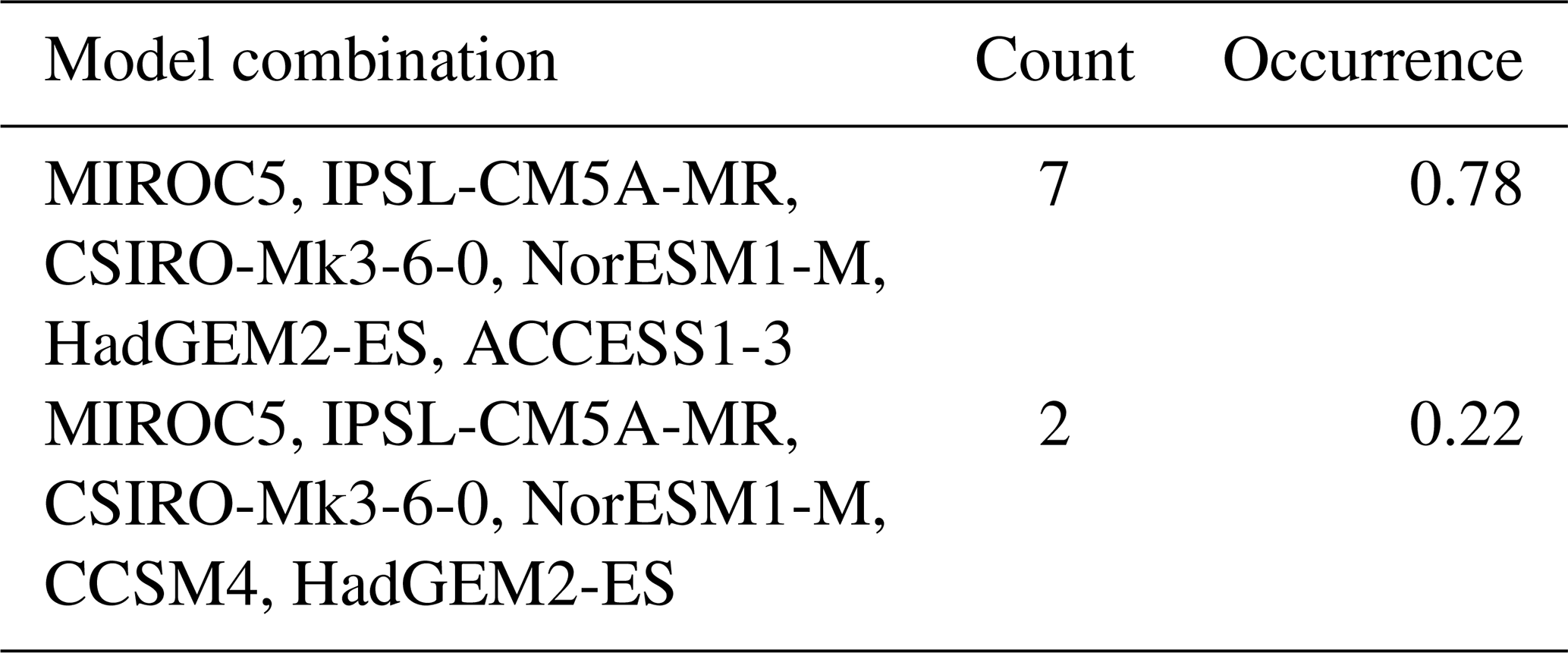
Table C8Absolute and relative occurrence of each individual model included in the Antarctica top three combinations presented in Table C7.

The supporting data are available at https://doi.org/10.5281/zenodo.3367347 (Barthel et al., 2019).
AB, CA, CML, NJ, TH, HG, HS, FS, and SN designed the study and the evaluation methodology. AB, CA and HG performed analysis on data provided by CA, CML, NJ, TH, and TJB. AB prepared the manuscript with contributions from all co-authors.
The authors declare that they have no conflict of interest.
This article is part of the special issue “The Ice Sheet Model Intercomparison Project for CMIP6 (ISMIP6)”. It is not associated with a conference.
Alice Barthel was supported by the U.S. Department of Energy (DOE) Office of Science Regional and Global Model Analysis (RGMA) component of the Earth and Environmental System Modeling (EESM) program (HiLAT-RASM project) and the DOE Office of Science (Biological and Environmental Research), Early Career Research program. Cecile Agosta was supported by the Agence Nationale de la Recherche Scientifique, project ANR-15-CE01-0015 (AC-AHC2) and by the Fondation Albert II de Monaco under the project Antarctic-Snow (2018–2020). Christopher M. Little acknowledges financial support from NSF grants 1513396 and 1744792. Tore Hatterman acknowledges financial support from Norwegian Research Council projects 231549 and 280727. Nicolas C. Jourdain's contribution was partly funded by the French National Research Agency (ANR) through the TROIS-AS (ANR-15-CE01-0005-01). Heiko Goelzer has received funding from the program of the Netherlands Earth System Science Centre (NESSC), financially supported by the Dutch Ministry of Education, Culture and Science (OCW) under grant no. 024.002.001. Helene Seroussi was supported by grants from the NASA Cryospheric Science, Sea Level Change Team, and Modeling Analysis and Prediction Program. Fiammetta Straneo acknowledges financial support from NSF grants 1756272 and 1916566. Thomas J. Bracegirdle acknowledges support from NERC grant NE/N018486/1 and the AntClim21 Scientific Research Programme of the Scientific Committee on Antarctic Research. We thank the Climate and Cryosphere (CliC) effort, which provided support for ISMIP6 through sponsoring of workshops, hosting the ISMIP6 website and wiki, and promoting ISMIP6. We acknowledge the World Climate Research Programme, which, through its Working Group on Coupled Modelling, coordinated and promoted CMIP5. We thank the climate modeling groups (listed in Table 1 of this paper) for producing and making available their model output, the Earth System Grid Federation (ESGF) for archiving the CMIP data and providing access, the University at Buffalo for ISMIP6 data distribution and upload, and the multiple funding agencies who support CMIP5 and CMIP6 and ESGF. We thank the ISMIP6 steering committee, the ISMIP6 model selection group, and ISMIP6 dataset preparation group for their continuous engagement in defining ISMIP6 and for discussions and feedback, with particular thanks to Donald Slater and Denis Felikson. This is ISMIP6 publication number 5.
This research has been supported by the U.S. Department of Energy, Office of Science (RGMA program and BER program grant), the Agence Nationale de la Recherche (grant no. ANR-15-CE01-0015 (AC-AHC2)), the Fondation Albert II de Monaco (project Antarctic-Snow grant), the National Science Foundation, Division of Polar Programs (grant nos. 1513396 and 1744792), the Agence Nationale de la Recherche (grant no. ANR-15-CE01-0005-01), the Netherlands Earth System Science Centre (grant no. 024.002.001), the NERC (grant no. NE/N018486/1), the National Science Foundation (grant nos. 1756272 and 1916566), NASA (Sea Level Change Team, and Modeling Analysis and Prediction Program grant), and the Norwegian Research Council (grant nos. 231549 and 280727).
This paper was edited by Ginny Catania and reviewed by two anonymous referees.
Agosta, C., Fettweis, X., and Datta, R.: Evaluation of the CMIP5 models in the aim of regional modelling of the Antarctic surface mass balance, The Cryosphere, 9, 2311–2321, https://doi.org/10.5194/tc-9-2311-2015, 2015. a, b, c, d, e, f, g
Agosta, C., Amory, C., Kittel, C., Orsi, A., Favier, V., Gallée, H., van den Broeke, M. R., Lenaerts, J. T. M., van Wessem, J. M., van de Berg, W. J., and Fettweis, X.: Estimation of the Antarctic surface mass balance using the regional climate model MAR (1979–2015) and identification of dominant processes, The Cryosphere, 13, 281–296, https://doi.org/10.5194/tc-13-281-2019, 2019. a
Andrews, L. C., Catania, G. A., Hoffman, M. J., Gulley, J. D., Lüthi, M. P., Ryser, C., Hawley, R. L., and Neumann, T. A.: Direct observations of evolving subglacial drainage beneath the Greenland Ice Sheet, Nature, 514, 80, https://doi.org/10.1038/nature13796, 2014. a
Asay-Davis, X. S., Jourdain, N. C., and Nakayama, Y.: Developments in Simulating and Parameterizing Interactions Between the Southern Ocean and the Antarctic Ice Sheet, Curr. Clim. Change Rep., 3, 316–329, https://doi.org/10.1007/s40641-017-0071-0, 2017. a
Banwell, A. F., MacAyeal, D. R., and Sergienko, O. V.: Breakup of the Larsen B Ice Shelf triggered by chain reaction drainage of supraglacial lakes, Geophys. Res. Lett., 40, 5872–5876, 2013. a
Barletta, V. R., Bevis, M., Smith, B. E., Wilson, T., Brown, A., Bordoni, A., Willis, M., Khan, S. A., Rovira-Navarro, M., Dalziel, I., Smalley, R., Kendrick, E., Konfal, S., Caccamise, D. J., Aster, R. C., Nyblade, A., and Wiens, D. A.: Observed rapid bedrock uplift in Amundsen Sea Embayment promotes ice-sheet stability, Science, 360, 1335–1339, https://doi.org/10.1126/science.aao1447, 2018. a
Barthel, A., Agosta, C., Hatterman, T., Jourdain, N., and Bracegirdle, T.: Dataset for ISMIP6 CMIP5 model selection, Zenodo, https://doi.org/10.5281/zenodo.3367347, 2019. a
Bindschadler, R. A., Nowicki, S., Abe-Ouchi, A., Aschwanden, A., Choi, H., Fastook, J., Granzow, G., Greve, R., Gutowski, G., Herzfeld, U., Jackson, C., Johnson, J., Khroulev, C., Levermann, A., Lipscomb, W. H., Martin, M. A., Morlighem, M., Parizek, B. R., Pollard, D., Price, S. F., Ren, D., Saito, F., Sato, T., Seddik, H., Seroussi, H., Takahashi, K., Walker, R., and Wang, W. L.: Ice-sheet model sensitivities to environmental forcing and their use in projecting future sea level (the SeaRISE project), J. Glaciol., 59, 195–224, https://doi.org/10.3189/2013JoG12J125, 2013. a
Bracegirdle, T. J. and Marshall, G. J.: The Reliability of Antarctic Tropospheric Pressure and Temperature in the Latest Global Reanalyses, J. Climate, 25, 7138–7146, https://doi.org/10.1175/JCLI-D-11-00685.1, 2012. a
Bracegirdle, T. J., Stephenson, D. B., Turner, J., and Phillips, T.: The importance of sea ice area biases in 21st century multimodel projections of Antarctic temperature and precipitation, Geophys. Res. Lett., 42, 10832–10839, https://doi.org/10.1002/2015gl067055, 2015. a, b
Bracegirdle, T. J., Hyder, P., and Holmes, C. R.: CMIP5 Diversity in Southern Westerly Jet Projections Related to Historical Sea Ice Area: Strong Link to Strengthening and Weak Link to Shift, J. Climate, 31, 195–211, https://doi.org/10.1175/JCLI-D-17-0320.1, 2018. a, b, c, d, e
Bromwich, D. H., Nicolas, J. P., and Monaghan, A. J.: An Assessment of Precipitation Changes over Antarctica and the Southern Ocean since 1989 in Contemporary Global Reanalyses *, J. Climate, 24, 4189–4209, https://doi.org/10.1175/2011JCLI4074.1, 2011. a
Dee, D. P., Uppala, S. M., Simmons, A. J., Berrisford, P., Poli, P., Kobayashi, S., Andrae, U., Balmaseda, M. A., Balsamo, G., Bauer, P., Bechtold, P., Beljaars, A. C. M., van de Berg, L., Bidlot, J., Bormann, N., Delsol, C., Dragani, R., Fuentes, M., Geer, A. J., Haimberger, L., Healy, S. B., Hersbach, H., Hólm, E. V., Isaksen, L., Kållberg, P., Köhler, M., Matricardi, M., McNally, A. P., Monge-Sanz, B. M., Morcrette, J.-J., Park, B.-K., Peubey, C., de Rosnay, P., Tavolato, C., Thépaut, J.-N., and Vitart, F.: The ERA-Interim reanalysis: configuration and performance of the data assimilation system, Q. J. Roy. Meteorol. Soc., 137, 553–597, https://doi.org/10.1002/qj.828, 2011. a
Dinniman, M. S., Asay-Davis, X. S., Galton-Fenzi, B. K., Holland, P. R., Jenkins, A., and Timmermann, R.: Modeling ice shelf/ocean interaction in Antarctica: A review, Oceanography, 29, 144–153, 2016. a, b
Domack, E., Duran, D., Leventer, A., Ishman, S., Doane, S., McCallum, S., Amblas, D., Ring, J., Gilbert, R., and Prentice, M.: Stability of the Larsen B ice shelf on the Antarctic Peninsula during the Holocene epoch, Nature, 436, 681–685, https://doi.org/10.1038/nature03908, 2005. a
Dutheil, C., Bador, M., Lengaigne, M., Lefèvre, J., Jourdain, N. C., Vialard, J., Jullien, S., Peltier, A., and Menkes, C.: Impact of surface temperature biases on climate change projections of the South Pacific Convergence Zone, Clim. Dynam., 53, 1–23, https://doi.org/10.1007/s00382-019-04692-6, 2019. a
Favier, V., Krinner, G., Amory, C., Gallée, H., Beaumet, J., and Agosta, C.: Antarctica-Regional Climate and Surface Mass Budget, Curr. Clim. Change Rep., 3, 303–315, https://doi.org/10.1007/s40641-017-0072-z, 2017. a
Ferry, N., Parent, L., Garric, G., Bricaud, C., Testut, C.-E., Galloudec, O. L., Lellouche, J.-M., Drévillon, M., Greiner, E., Barnier, B., Molines, J.-M., Jourdain, N., Guinehut, S., Cabanes, C., and Zawadzki, L.: GLORYS2V1 global ocean reanalysis of the altimetric era (1993-2009) at meso scale, Mercator Ocean Q. News., 44, 28–39, 2012. a
Fettweis, X., Franco, B., Tedesco, M., van Angelen, J. H., Lenaerts, J. T. M., van den Broeke, M. R., and Gallée, H.: Estimating the Greenland ice sheet surface mass balance contribution to future sea level rise using the regional atmospheric climate model MAR, The Cryosphere, 7, 469–489, https://doi.org/10.5194/tc-7-469-2013, 2013. a, b, c
Fettweis, X., Box, J. E., Agosta, C., Amory, C., Kittel, C., Lang, C., van As, D., Machguth, H., and Gallée, H.: Reconstructions of the 1900–2015 Greenland ice sheet surface mass balance using the regional climate MAR model, The Cryosphere, 11, 1015–1033, https://doi.org/10.5194/tc-11-1015-2017, 2017. a, b, c
Franco, B., Fettweis, X., and Erpicum, M.: Future projections of the Greenland ice sheet energy balance driving the surface melt, The Cryosphere, 7, 1–18, https://doi.org/10.5194/tc-7-1-2013, 2013. a
Frieler, K., Clark, P. U., He, F., Buizert, C., Reese, R., Ligtenberg, S. R. M., van den Broeke, M. R. v. d., Winkelmann, R., and Levermann, A.: Consistent evidence of increasing Antarctic accumulation with warming, Nat. Clim. Change, 5, 348–352, https://doi.org/10.1038/nclimate2574, 2015. a
Fyke, J., Lenaerts, J. T. M., and Wang, H.: Basin-scale heterogeneity in Antarctic precipitation and its impact on surface mass variability, The Cryosphere, 11, 2595–2609, https://doi.org/10.5194/tc-11-2595-2017, 2017. a
Good, S. A., Martin, M. J., and Rayner, N. A.: EN4: Quality controlled ocean temperature and salinity profiles and monthly objective analyses with uncertainty estimates, J. Geophys. Res.-Oceans, 118, 6704–6716, https://doi.org/10.1002/2013JC009067, 2013. a
Hellmer, H. H., Kauker, F., Timmermann, R., Determann, J., and Rae, J.: Twenty-first-century warming of a large Antarctic ice-shelf cavity by a redirected coastal current, Nature, 485, 225–228, https://doi.org/10.1038/nature11064, 2012. a
Holland, M. M., Landrum, L., Kostov, Y., and Marshall, J.: Sensitivity of Antarctic sea ice to the Southern Annular Mode in coupled climate models, Clim. Dynam., 49, 1813–1831, https://doi.org/10.1007/s00382-016-3424-9, 2017. a
Huai, B., Wang, Y., Ding, M., Zhang, J., and Dong, X.: An assessment of recent global atmospheric reanalyses for Antarctic near surface air temperature, Atmos. Res., 226, 181–191, 2019. a
Jourdain, N. C., Asay-Davis, X., Hattermann, T., Straneo, F., Seroussi, H., Little, C. M., and Nowicki, S.: A protocol for calculating basal melt rates in the ISMIP6 Antarctic ice sheet projections, The Cryosphere Discuss., https://doi.org/10.5194/tc-2019-277, in review, 2019. a
Kendrick, A. K., Schroeder, D. M., Chu, W., Young, T. J., Christoffersen, P., Todd, J., Doyle, S. H., Box, J. E., Hubbard, A., Hubbard, B., Brennan, P. V., Nicholls, K. W., and Lok, L. B.: Surface Meltwater Impounded by Seasonal Englacial Storage in West Greenland, Geophys. Res. Lett., 45, 10474–10481, https://doi.org/10.1029/2018gl079787, 2018. a
Khan, S. A., Kjær, K. H., Bevis, M., Bamber, J. L., Wahr, J., Kjeldsen, K. K., Bjørk, A. A., Korsgaard, N. J., Stearns, L. A., van den Broeke, M. R., Liu, L., Larsen, N. K., and Muresan, I. S.: Sustained mass loss of the northeast Greenland ice sheet triggered by regional warming, Nat. Clim. Change, 4, 292–299, https://doi.org/10.1038/nclimate2161, 2014. a
Kimura, S., Jenkins, A., Regan, H., Holland, P. R., Assmann, K. M., Whitt, D. B., Van Wessem, M., van de Berg, W. J., Reijmer, C. H., and Dutrieux, P.: Oceanographic Controls on the Variability of Ice-Shelf Basal Melting and Circulation of Glacial Meltwater in the Amundsen Sea Embayment, Antarctica, J. Geophys. Res.-Oceans, 122, 10131–10155, https://doi.org/10.1002/2017JC012926, 2017. a
Knutti, R., Masson, D., and Gettelman, A.: Climate model genealogy: Generation CMIP5 and how we got there, Geophys. Res. Lett., 40, 1194–1199, https://doi.org/10.1002/grl.50256, 2013. a
Krinner, G. and Flanner, M. G.: Striking stationarity of large-scale climate model bias patterns under strong climate change, P. Natl. Acad. Sci. USA, 115, 9462–9466, https://doi.org/10.1073/pnas.1807912115, 2018. a
Krinner, G., Largeron, C., Ménégoz, M., Agosta, C., and Brutel-Vuilmet, C.: Oceanic Forcing of Antarctic Climate Change: A Study Using a Stretched-Grid Atmospheric General Circulation Model, J. Climate, 27, 5786–5800, https://doi.org/10.1175/JCLI-D-13-00367.1, 2014. a
Levermann, A., Winkelmann, R., Nowicki, S., Fastook, J. L., Frieler, K., Greve, R., Hellmer, H. H., Martin, M. A., Meinshausen, M., Mengel, M., Payne, A. J., Pollard, D., Sato, T., Timmermann, R., Wang, W. L., and Bindschadler, R. A.: Projecting Antarctic ice discharge using response functions from SeaRISE ice-sheet models, Earth Syst. Dynam., 5, 271–293, https://doi.org/10.5194/esd-5-271-2014, 2014. a, b
Little, C. M. and Urban, N. M.: CMIP5 temperature biases and 21st century warming around the Antarctic coast, Ann. Glaciol., 57, 69–78, https://doi.org/10.1017/aog.2016.25, 2016. a
Locarnini, R. A., Mishonov, A. V., Antonov, J. I., Boyer, T. P., Garcia, H. E., Baranova, O. K., Zweng, M. M., Paver, C. R., Reagan, J. R., Johnson, D. R., Hamilton, M., and Seidov, D.: World Ocean Atlas 2013, Volume 1: Temperature, NOAA Atlas NESDIS 73, 2013. a
Locarnini, R. A., Mishonov, A. V., Baranova, O. K., Boyer, T. P., Zweng, M. M., Garcia, H. E., Reagan, J. R., Seidov, D., Weathers, K. W., Paver, C. R., and Smolyar, I.: World Ocean Atlas 2018, Volume 1: Temperature, NOAA Atlas NESDIS 81, available at: https://data.nodc.noaa.gov/woa/WOA18/DOC/woa18_vol1.pdf (last access: 9 February 2020), 2019. a
Meijers, A. J. S., Shuckburgh, E., Bruneau, N., Sallee, J.-B., Bracegirdle, T. J., and Wang, Z.: Representation of the Antarctic Circumpolar Current in the CMIP5 climate models and future changes under warming scenarios, J. Geophys. Res.-Oceans, 117, C12008, https://doi.org/10.1029/2012JC008412, 2012. a
Morlighem, M., Williams, C. N., Rignot, E., An, L., Arndt, J. E., Bamber, J. L., Catania, G., Chauché, N., Dowdeswell, J. A., Dorschel, B., Fenty, I., Hogan, K., Howat, I., Hubbard, A., Jakobsson, M., Jordan, T. M., Kjeldsen, K. K., Millan, R., Mayer, L., Mouginot, J., Noël, B. P. Y., O'Cofaigh, C., Palmer, S., Rysgaard, S., Seroussi, H., Siegert, M. J., Slabon, P., Straneo, F., van den Broeke, M. R., Weinrebe, W., Wood, M., and Zinglersen, K. B.: BedMachine v3: Complete bed topography and ocean bathymetry mapping of Greenland from multibeam echo sounding combined with mass conservation, Geophys. Res. Lett., 44, 11051–11061, 2017. a
Mouginot, J., Rignot, E., and Scheuchl, B.: Sustained increase in ice discharge from the Amundsen Sea Embayment, West Antarctica, from 1973 to 2013, Geophys. Res. Lett., 41, 1576–1584, https://doi.org/10.1002/2013GL059069, 2014. a, b
Mouginot, J., Rignot, E., Bjørk, A. A., van den Broeke, M., Millan, R., Morlighem, M., Noël, B., Scheuchl, B., and Wood, M.: Forty-six years of Greenland Ice Sheet mass balance from 1972 to 2018, P. Natl. Acad. Sci. USA, 116, 9239–9244, https://doi.org/10.1073/pnas.1904242116, 2019. a
Naughten, K. A., Meissner, K. J., Galton-Fenzi, B. K., England, M. H., Timmermann, R., Hellmer, H. H., Hattermann, T., and Debernard, J. B.: Intercomparison of Antarctic ice-shelf, ocean, and sea-ice interactions simulated by MetROMS-iceshelf and FESOM 1.4, Geosci. Model Dev., 11, 1257–1292, https://doi.org/10.5194/gmd-11-1257-2018, 2018. a
Noël, B., Fettweis, X., van de Berg, W. J., van den Broeke, M. R., and Erpicum, M.: Sensitivity of Greenland Ice Sheet surface mass balance to perturbations in sea surface temperature and sea ice cover: a study with the regional climate model MAR, The Cryosphere, 8, 1871–1883, https://doi.org/10.5194/tc-8-1871-2014, 2014. a
Noël, B., van de Berg, W. J., van Wessem, J. M., van Meijgaard, E., van As, D., Lenaerts, J. T. M., Lhermitte, S., Kuipers Munneke, P., Smeets, C. J. P. P., van Ulft, L. H., van de Wal, R. S. W., and van den Broeke, M. R.: Modelling the climate and surface mass balance of polar ice sheets using RACMO2 – Part 1: Greenland (1958–2016), The Cryosphere, 12, 811–831, https://doi.org/10.5194/tc-12-811-2018, 2018. a, b
Nowicki, S.: ISMIP6 wiki page, available at: http://www.climate-cryosphere.org/wiki/index.php?title=ISMIP6_wiki_page#ISMIP6_Standalone_Ice_Sheet_Experiments (last access: 9 February 2020), 2019. a, b, c, d, e
Nowicki, S. M. J., Payne, A., Larour, E., Seroussi, H., Goelzer, H., Lipscomb, W., Gregory, J., Abe-Ouchi, A., and Shepherd, A.: Ice Sheet Model Intercomparison Project (ISMIP6) contribution to CMIP6, Geosci. Model Dev., 9, 4521–4545, https://doi.org/10.5194/gmd-9-4521-2016, 2016. a, b
Palerme, C., Genthon, C., Claud, C., Kay, J. E., Wood, N. B., and L’Ecuyer, T.: Evaluation of current and projected Antarctic precipitation in CMIP5 models, Clim. Dynam., 48, 225–239, 2017. a
Pattyn, F., Perichon, L., Durand, G., Favier, L., Gagliardini, O., Hindmarsh, R. C., Zwinger, T., Albrecht, T., Cornford, S., Docquier, D., Fürst, J. J., Goldberg, D., Gudmundsson, G. H., Humbert, A., Hütten, M., Huybrechts, P., Jouvet, G., Kleiner, T., Larour, E., Martin, D., Morlighem, M., Payne, A. J., Pollard, D., Rückamp, M., Rybak, O., Seroussi, H., Thoma, M., and Wilkens, N.: Grounding-line migration in plan-view marine ice-sheet models: Results of the ice2sea MISMIP3d intercomparison, J. Glaciol., 59, 410–422, https://doi.org/10.3189/2013JoG12J129, 2013. a
Rignot, E., Casassa, G., Gogineni, P., Krabill, W., Rivera, A., and Thomas, R.: Accelerated ice discharge from the Antarctic Peninsula following the collapse of Larsen B ice shelf, Geophys. Res. Lett., 31, 18, https://doi.org/10.1029/2004gl020697, 2004. a
Roquet, F., Guinet, C., Charrassin, J.-B., Costa, D. P., Kovacs, K. M., Lydersen, C., Bornemann, H., Bester, M. N., Muelbert, M. C., Hindell, M. A., McMahon, C. R., Harcourt, R., Boehme, L., and Fedak, M. A.: MEOP-CTD in-situ data collection: a Southern ocean Marine-mammals calibrated sea water temperatures and salinities observations, SEANOE, https://doi.org/10.17882/45461, 2018. a
Russell, J. L., Kamenkovich, I., Bitz, C., Ferrari, R., Gille, S. T., Goodman, P. J., Hallberg, R., Johnson, K., Khazmutdinova, K., Marinov, I., Mazloff, M., Riser, S., Sarmiento, J. L., Speer, K., Talley, L. D., and Wanninkhof, R.: Metrics for the evaluation of the southern ocean in coupled climate models and earth system models, J. Geophys. Res.-Oceans, 123, 3120–3143, https://doi.org/10.1002/2017JC013461, 2018. a
Sallée, J., Shuckburgh, E., Bruneau, N., Meijers, a. J. S., Bracegirdle, T. J., Wang, Z., and Roy, T.: Assessment of Southern Ocean water mass circulation and characteristics in CMIP5 models: Historical bias and forcing response, J. Geophys. Res.-Oceans, 118, 1830–1844, https://doi.org/10.1002/jgrc.20135, 2013. a
Sanderson, B. M., Knutti, R., and Caldwell, P.: Addressing Interdependency in a Multimodel Ensemble by Interpolation of Model Properties, J. Climate, 28, 5150–5170, https://doi.org/10.1175/JCLI-D-14-00361.1, 2015a. a
Sanderson, B. M., Knutti, R., and Caldwell, P.: A Representative Democracy to Reduce Interdependency in a Multimodel Ensemble, J. Climate, 28, 5171–5194, https://doi.org/10.1175/JCLI-D-14-00362.1, 2015b. a
Schmidtko, S., Heywood, K. J., Thompson, A. F., and Aoki, S.: Multidecadal warming of Antarctic waters, Science, 346, 1227–1231, https://doi.org/10.1126/science.1256117, 2014. a
Shepherd, A., Ivins, E., Rignot, E., Smith, B., Broeke, M. v. d., Velicogna, I., Whitehouse, P., Briggs, K., Joughin, I., Krinner, G., Nowicki, S., Payne, T., Scambos, T., Schlegel, N., A, G., Agosta, C., Ahlstrøm, A., Babonis, G., Barletta, V., Blazquez, A., Bonin, J., Csatho, B., Cullather, R., Felikson, D., Fettweis, X., Forsberg, R., Gallee, H., Gardner, A., Gilbert, L., Groh, A., Gunter, B., Hanna, E., Harig, C., Helm, V., Horvath, A., Horwath, M., Khan, S., Kjeldsen, K. K., Konrad, H., Langen, P., Lecavalier, B., Loomis, B., Luthcke, S., McMillan, M., Melini, D., Mernild, S., Mohajerani, Y., Moore, P., Mouginot, J., Moyano, G., Muir, A., Nagler, T., Nield, G., Nilsson, J., Noel, B., Otosaka, I., Pattle, M. E., Peltier, W. R., Pie, N., Rietbroek, R., Rott, H., Sandberg-Sørensen, L., Sasgen, I., Save, H., Scheuchl, B., Schrama, E., Schröder, L., Seo, K.-W., Simonsen, S., Slater, T., Spada, G., Sutterley, T., Talpe, M., Tarasov, L., Berg, W. J. v. d., Wal, W. v. d., Wessem, M. v., Vishwakarma, B. D., Wiese, D., and Wouters, B.: Mass balance of the Antarctic Ice Sheet from 1992 to 2017, Nature, 558, 219–222, https://doi.org/10.1038/s41586-018-0179-y, 2018. a
Slater, D. A., Straneo, F., Felikson, D., Little, C. M., Goelzer, H., Fettweis, X., and Holte, J.: Estimating Greenland tidewater glacier retreat driven by submarine melting, The Cryosphere, 13, 2489–2509, https://doi.org/10.5194/tc-13-2489-2019, 2019. a, b, c
Stewart, A. L., Klocker, A., and Menemenlis, D.: Circum-Antarctic shoreward heat transport derived from an eddy-and tide-resolving simulation, Geophys. Res. Lett., 45, 834–845, 2018. a
Straneo, F. and Cenedese, C.: The Dynamics of Greenland's Glacial Fjords and Their Role in Climate, Ann. Rev. Mar. Sci., 7, 89–112, https://doi.org/10.1146/annurev-marine-010213-135133, pMID: 25149564, 2015. a
Straneo, F., Sutherland, D. A., Holland, D., Gladish, C., Hamilton, G. S., Johnson, H. L., Rignot, E., Xu, Y., and Koppes, M.: Characteristics of ocean waters reaching Greenland's glaciers, Ann. Glaciol., 53, 202–210, https://doi.org/10.3189/2012AoG60A059, 2012. a, b
Tedesco, M. and Fettweis, X.: 21st century projections of surface mass balance changes for major drainage systems of the Greenland ice sheet, Environm. Res. Lett., 7, 045405, https://doi.org/10.1088/1748-9326/7/4/045405, 2012. a
Thompson, A. F., Stewart, A. L., Spence, P., and Heywood, K. J.: The Antarctic Slope Current in a Changing Climate, Rev. Geophys., 56, 741–770, https://doi.org/10.1029/2018RG000624, 2018. a, b, c
Timmermann, R. and Goeller, S.: Response to Filchner–Ronne Ice Shelf cavity warming in a coupled ocean–ice sheet model – Part 1: The ocean perspective, Ocean Sci., 13, 765–776, 2017. a, b
Trusel, L. D., Frey, K. E., Das, S. B., Munneke, P. K., and Van Den Broeke, M. R.: Satellite-based estimates of Antarctic surface meltwater fluxes, Geophys. Res. Lette., 40, 6148–6153, 2013. a
Trusel, L. D., Frey, K. E., Das, S. B., Karnauskas, K. B., Munneke, P. K., Van Meijgaard, E., and Van Den Broeke, M. R.: Divergent trajectories of Antarctic surface melt under two twenty-first-century climate scenarios, Nat. Geosci., 8, 927, 2015. a
Trusel, L. D., Das, S. B., Osman, M. B., Evans, M. J., Smith, B. E., Fettweis, X., McConnell, J. R., Noël, B. P. Y., and van den Broeke, M. R. v. d.: Nonlinear rise in Greenland runoff in response to post-industrial Arctic warming, Nature, 564, 104–108, https://doi.org/10.1038/s41586-018-0752-4, 2018. a
van den Broeke, M.: Strong surface melting preceded collapse of Antarctic Peninsula ice shelf, Geophys. Res. Lett., 32, L12815, 2005. a
van Wessem, J. M., van de Berg, W. J., Noël, B. P. Y., van Meijgaard, E., Amory, C., Birnbaum, G., Jakobs, C. L., Krüger, K., Lenaerts, J. T. M., Lhermitte, S., Ligtenberg, S. R. M., Medley, B., Reijmer, C. H., van Tricht, K., Trusel, L. D., van Ulft, L. H., Wouters, B., Wuite, J., and van den Broeke, M. R.: Modelling the climate and surface mass balance of polar ice sheets using RACMO2 – Part 2: Antarctica (1979–2016), The Cryosphere, 12, 1479–1498, https://doi.org/10.5194/tc-12-1479-2018, 2018. a
Velicogna, I.: Increasing rates of ice mass loss from the Greenland and Antarctic ice sheets revealed by GRACE, Geophys. Res. Lett., 36, 2–5, https://doi.org/10.1029/2009GL040222, 2009. a
Yin, J., Overpeck, J. T., Griffies, S. M., Hu, A., Russell, J. L., and Stouffer, R. J.: Different magnitudes of projected subsurface ocean warming around Greenland and Antarctica, Nat. Geosci., 4, 524, https://doi.org/10.1038/ngeo1189, 2011. a
Zwally, H. J., Li, J., Brenner, A. C., Beckley, M., Cornejo, H. G., DiMarzio, J., Giovinetto, M. B., Neumann, T. A., Robbins, J., Saba, J. L., Yi, D., and Wang, W.: Greenland ice sheet mass balance: distribution of increased mass loss with climate warming; 2003–07 versus 1992–2002, J. Glaciol., 57, 88–102, https://doi.org/10.3189/002214311795306682, 2011. a
- Abstract
- Introduction and objectives
- Data and methods
- Results for Antarctica
- Results for Greenland
- Discussion
- Conclusions
- Appendix A: Robustness of historical ranking
- Appendix B: Projected 21C ocean warming
- Appendix C: Robustness of model selection
- Data availability
- Author contributions
- Competing interests
- Special issue statement
- Acknowledgements
- Financial support
- Review statement
- References